the Creative Commons Attribution 4.0 License.
the Creative Commons Attribution 4.0 License.
 | 06 Oct 2022
Comparison of particle number size distribution trends in ground measurements and climate models
Harri Kokkola
Taina Yli-Juuti
Tero Mielonen
Thomas Kühn
Tuomo Nieminen
Simo Heikkinen
Tuuli Miinalainen
Tommi Bergman
Ken Carslaw
Stefano Decesari
Markus Fiebig
Tareq Hussein
Niku Kivekäs
Radovan Krejci
Markku Kulmala
Ari Leskinen
Andreas Massling
Nikos Mihalopoulos
Jane P. Mulcahy
Steffen M. Noe
Twan van Noije
Fiona M. O'Connor
Colin O'Dowd
Dirk Olivie
Jakob B. Pernov
Tuukka Petäjä
Øyvind Seland
Michael Schulz
Catherine E. Scott
Henrik Skov
Erik Swietlicki
Thomas Tuch
Alfred Wiedensohler
Annele Virtanen
Santtu Mikkonen
Despite a large number of studies, out of all drivers of radiative forcing, the effect of aerosols has the largest uncertainty in global climate model radiative forcing estimates. There have been studies of aerosol optical properties in climate models, but the effects of particle number size distribution need a more thorough inspection. We investigated the trends and seasonality of particle number concentrations in nucleation, Aitken, and accumulation modes at 21 measurement sites in Europe and the Arctic. For 13 of those sites, with longer measurement time series, we compared the field observations with the results from five climate models, namely EC-Earth3, ECHAM-M7, ECHAM-SALSA, NorESM1.2, and UKESM1. This is the first extensive comparison of detailed aerosol size distribution trends between in situ observations from Europe and five earth system models (ESMs). We found that the trends of particle number concentrations were mostly consistent and decreasing in both measurements and models. However, for many sites, climate models showed weaker decreasing trends than the measurements. Seasonal variability in measured number concentrations, quantified by the ratio between maximum and minimum monthly number concentration, was typically stronger at northern measurement sites compared to other locations. Models had large differences in their seasonal representation, and they can be roughly divided into two categories: for EC-Earth and NorESM, the seasonal cycle was relatively similar for all sites, and for other models the pattern of seasonality varied between northern and southern sites. In addition, the variability in concentrations across sites varied between models, some having relatively similar concentrations for all sites, whereas others showed clear differences in concentrations between remote and urban sites. To conclude, although all of the model simulations had identical input data to describe anthropogenic mass emissions, trends in differently sized particles vary among the models due to assumptions in emission sizes and differences in how models treat size-dependent aerosol processes. The inter-model variability was largest in the accumulation mode, i.e. sizes which have implications for aerosol–cloud interactions. Our analysis also indicates that between models there is a large variation in efficiency of long-range transportation of aerosols to remote locations. The differences in model results are most likely due to the more complex effect of different processes instead of one specific feature (e.g. the representation of aerosol or emission size distributions). Hence, a more detailed characterization of microphysical processes and deposition processes affecting the long-range transport is needed to understand the model variability.
- Article
(10013 KB) - Full-text XML
-
Supplement
(7714 KB) - BibTeX
- EndNote


Atmospheric aerosols form one of the most important components that cool the climate, counteracting heating by increased greenhouse gas concentrations (Forster et al., 2021). Aerosol–radiation interactions (ARIs) and aerosol–cloud interactions (ACIs) greatly depend on particle concentration, size distribution, and chemical properties and altogether their ability to activate to cloud droplets. On the other hand, the ability of large-scale climate models to predict the aerosol direct and indirect radiative forcing depends mainly on their ability to describe the spatial and temporal distribution and characteristics of the atmospheric aerosol population. Especially the strength of cooling due to ACI depends on the number concentration of particles large enough to activate to cloud droplets (Dusek et al., 2006). The ability of global-scale models to reproduce the trends of these particles is important for reproducing the changes in aerosol radiative forcing, and further on, diagnosing the radiative forcing from anthropogenic emissions. Improvement of aerosol radiative forcing estimates, which are still the most uncertain part of total radiative forcing estimates (Forster et al., 2021), would improve the estimate of total radiative forcing, the climate sensitivity, and future climate change (Myhre et al., 2013).
It is likely that there will be changes in trends of aerosol concentrations in future. It has been proposed that both air pollution and climate change mitigation measures will lead to decreased emissions of anthropogenic aerosols (Smith and Bond, 2014). In addition, a global-warming-driven temperature increase affects the emissions of biogenic volatile organic compounds (BVOCs) and formation of secondary organic aerosol and through that concentrations and size distribution characteristics of atmospheric aerosols (Arneth et al., 2010; Hellén et al., 2018; Mielonen et al., 2012; Paasonen et al., 2013; Peñuelas and Staudt, 2010; Yli-Juuti et al., 2021). Atmospheric aerosols have already undergone significant changes caused by tightened air pollution control measures. For example, Hamed et al. (2010) showed a clear reduction in aerosol concentrations in Melpitz, Germany, between 1996 and 2006, which was associated with sulfur dioxide (SO2) emission reductions in Europe. Several other studies have reported significant changes in the atmospheric aerosol population showing clear negative trends in particle concentrations in different size ranges (Mikkonen et al., 2020; Sun et al., 2020) as well as for total number concentration and mass (Asmi et al., 2013; Collaud Coen et al., 2013). The change in aerosol optical properties has been consistent with these observations, with aerosol optical depth showing a decreasing trend over Europe and the Arctic (Breider et al., 2017; Collaud Coen et al., 2013, 2020; Schmale et al., 2022).
To decrease the uncertainty in climate models related to ARI and ACI, model constraints and comparisons of observations and models are needed. Observations of particle number concentrations and their optical properties, as well as radiation measurements, help to constrain how well climate models simulate the climate effects of aerosols. Storelvmo et al. (2018) showed that models from the 5th Coupled Model Intercomparison Project (CMIP5) do not reproduce the observed trends in incoming surface solar radiation (SSR). Moseid et al. (2020) showed that the same holds also for the CMIP6 models. Since SSR is affected by aerosol extinction and cloud cover, the analysis of Moseid et al. (2020) indicated that the discrepancy between models and observations was related, at least partly, to erroneous aerosol and aerosol precursor emission inventories. Mortier et al. (2020) studied the trends of particle optical properties and found that the trends were mostly decreasing for measured optical parameters, and climate models mainly showed relatively similar trends. However, models usually underestimate aerosol optical parameters such as optical thickness and scattering (Gliß et al., 2021). These findings indicate a need for further analysis comparing observed trends of the aerosol population with trends from global models.
Interpretation and analysis of comparison of in situ aerosol observations with global model outputs is not straightforward due to differing temporal and spatial scales represented. In situ measurements represent one point, while a global-scale model simulates average aerosol properties within a grid box, which can be on the order of 100 km in horizontal resolution and on the order of a few tens of metres in the vertical at the level of the observations. The differences in scale make one-to-one comparison of models and observations at a specific time incoherent, unless the in situ observations represent the mean value of the model grid box area well. On the other hand, the proximity of the observation site to emission sources, changes in local wind speed and direction, and the dynamics of the boundary layer can cause large fluctuations at the measurement site. This local variation cannot be captured with the coarse resolution of global models and may not be representative of a larger area. However, using long time series and a large number of observational sites allows for bridging the gap between the scales (Schutgens et al., 2017). In addition, co-locating the observations and model data in time allows for a closer comparison of the two (Schutgens et al., 2016).
In this study, we perform an aerosol number size distribution trend analysis for observations from 21 European and Arctic sites, analyse the trends of particle mode properties (number concentration, geometric mean diameter, and geometric standard deviation), and compare 13 sites with simulations from five climate models over the period of 2001–2014. In addition, we compare the seasonal cycle representation of the models to the measured seasonal cycles in different regions of Europe.
We investigated the characteristics of particle number size distributions by separating the size distribution into log-normal modes (nucleation, Aitken, and accumulation mode). We analysed the number concentration, geometric mean diameter, and geometric standard deviation and their trends for sites representing polar (Villum, Zeppelin), Arctic remote (Pallas, Värriö), rural (Birkenes II, Hohenpeißenberg, Hyytiälä, Järvselja, Melpitz, San Pietro Capofiume), rural regional background (K-Puszta, Neuglobsow, Waldhof, Vavihill), urban (Annaberg-Buchholz, Helsinki, Leipzig, Puijo), coastal remote (Mace Head, Finokalia), and high-altitude (Schauinsland) environments. Finally, to evaluate how well current climate models can reproduce the observed aerosol physical trends and seasonal variability, we compared observations from 13 selected sites with results from 5 different climate models. The selection criterion for measurement–climate model comparison was for the measurement sites to provide at least 7 years of observational data between 2001 and 2014. See Sect. 2.1 and especially 2.1.1 for more details about measurement data and Sect. 2.1.4 and 2.2 for model comparison.
Measurement data sets differ in the reported aerosol size range and time resolution. Furthermore, the climate modelling data used (see Sect. 2.2) are averages over the grid boxes containing the coordinates of the respective measurement sites. It is therefore not straightforward to compare measurement data of different locations or to compare measured and modelled data. In order to make such comparisons meaningful, the data must be adjusted and modified in a consistent manner. In Sect. 2.1, we go through the data modification process used and explain and verify the chosen approaches and methods.
Daily and monthly averages of number size distribution parameters are used in the trend analysis (see Sect. 2.3). We are using the dynamic linear model (DLM) (Petris et al., 2009) to evaluate short-term changes in trends (based on the data of daily averages) and Sen–Theil estimators for long-term trend estimation (monthly averages) and comparing with the modelled trends of climate models (monthly averages). Seasonality of observed and climate model output number concentrations of each aerosol distribution mode is compared with seasonality metrics introduced in Rose et al. (2021) using monthly data.
2.1 Data from measurement sites
2.1.1 Measurement sites
Data sets used in this study are partly the same as in the study of Nieminen et al. (2018) and are supplemented by newer data from the Aerosol, Clouds and Trace Gases Research Infrastructure (ACTRIS) sites (https://www.actris.eu/, last access: 9 October 2019) and SmartSmear (https://smear.avaa.csc.fi/, last access: 31 July 2019). From ACTRIS sites, we have also included new sites that were not included in Nieminen et al. (2018) (Annaberg-Buchholz, Birkenes II, Leipzig, Neuglobsow, Puijo, Schauinsland, and Waldhof) and expanded the data length by including recent years that were missing in Nieminen et al. (2018). In addition, data from Villum Research Station at Station Nord (Villum) and some recent years' data from Puijo and San Pietro Capofiume were received directly from the research groups operating the sites.
In this study, we have used only long-term observations (minimum of 6 years of measurement data) of particle number size distributions. The length of the data sets (6–22 years) and corresponding data coverage (59.6 %–98.4 % of the days of the measurement period) varies between the sites (see Fig. S1 in the Supplement). The measurement sites used in this study are listed in Table 1. For model comparison, in turn, we have included only those sites that have at least 7 years of a common time period with the model simulations (2001–2014) and sufficient data coverage (i.e. coverage >50 % of days). In Table 1, the sites are presented in two separate lists: the first list shows the sites that are used in both trend analysis and comparisons of observational and model trends, and the second list shows sites that were used only in trend analysis.
Table 1Information of measurement sites used in this study. Site name, site environment type, coordinates, altitude in metres above sea level, time period, and size range (rounded to the nearest nanometre for minimum size and nearest 10 nm for maximum size) covered.
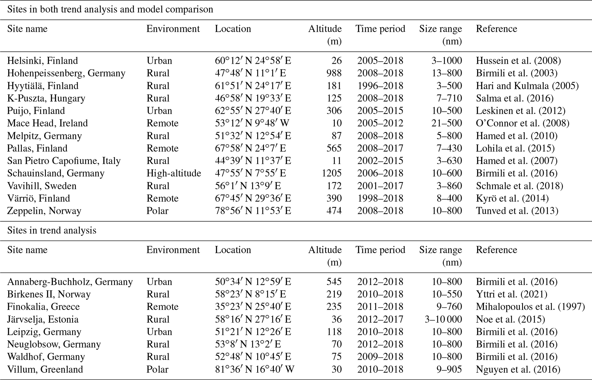
In this study we use commonly used site classes (polar, high-altitude, remote, rural, and urban) following Nieminen et al. (2018). Site environment classification of each site is adapted from Nieminen et al. (2018) for those sites that were included in their study. For other sites, we have used classifications from the literature (Sun et al., 2020, for German sites; Yttri et al., 2021, for Birkenes II; Leskinen et al., 2012, for Puijo; Schmale et al., 2018, for Vavihill; and Nguyen et al., 2016, for Villum) for environment classification and adjusted their classification according to Nieminen et al. (2018). A detailed description of each site, including the facility and environment descriptions, can be found in the literature (see Table 1).
It should be noted that there is a significant variation in the detected size ranges of the measurement instruments between the sites and within one site over the analysed time period (see Table 1). For those sites where the size range has varied over the investigated time period, we have limited the analysis only to the size range that has been measured over the whole analysis period. This size range is site-specific to maximize the number of data at each site. We have interpolated the data to site-specific, common size resolution; i.e. the size bins of size distribution data were the same for the whole time period. Measurement data size bins were interpolated because otherwise, the size bins can vary during time series, and hence, for example, the calculated modal and sectional representations (see definitions from Sect. 2.1.4) would be calculated from the different size bins.
When the in situ observations and large-scale models are compared, it is important to consider how representative the stations are for the larger areas surrounding them. The polar and remote sites (Zeppelin, Pallas, and Värriö) as well as rural site Hyytiälä can be considered to be representative of a larger regional fingerprint (Hari and Kulmala, 2005; Kyrö et al., 2014; Lohila et al., 2015; Tunved et al., 2013), and no large cities are located close to these sites. It should be noted that the Värriö site can be impacted by pollution transported from the Kola Peninsula mining and industrial areas (200–300 km north-east from the station) at times (Kyrö et al., 2014). Mace Head represents marine environment excellently when the air masses arrive from the Atlantic but on the other hand can be affected by the continental outflow as well (O'Connor et al., 2008). The urban sites Helsinki and Puijo (as urban sites in general) are affected by strong, local sources such as traffic or local industrial activity, and the diurnal variation in the representativeness to the larger areas might be significant (Hussein et al., 2008; Leskinen et al., 2012). The rural (Hohenpeißenberg, K-Puszta, Melpitz, San Pietro Capofiume, Vavihill) sites represent European background well, but their representativeness for the model grid box depends on the placement of the grid box and on how large the fraction of the grid box covered by large cities is. It should be noted that Hohenpeißenberg is located at high altitude (988 m) and is classified as a mountain site in some of the earlier studies (e.g. Rose et al., 2021), while Nieminen et al. (2018) classified it as a rural site.
2.1.2 Fitting of log-normal modes to particle number size distributions
Multimodal log-normal size distributions were fitted to the measured data, and the trend analysis was performed on the mode parameters. We fitted three log-normal modes (nucleation, Aitken, and accumulation) to the measured data. Before fitting the modes, we first performed a visual examination of the size distribution time series to detect clear errors in the data that could affect the results of the fitting process, e.g. the absence of some modes in the fit due to problems in the data. For example, if a substantial fraction (over 20 % of the size bins) of the number size distribution was not measured during a specific size distribution measurement, the whole distribution was removed. In addition, measurement sites have performed the quality checks routinely on the data before transferring data to the database or server.
Modes were fitted for each particle size distribution using an automatic mode-fitting algorithm (Hussein et al., 2005). Briefly, the algorithm fits a combination of one to three log-normal distributions to the particle number size distribution data separately for each time step at each location. The algorithm assumes three log-normal modes as a starting point and automatically reduces the number of modes if any of the overlapping conditions for modes is true (for more details, see Hussein et al., 2005). For each mode, the algorithm returns three parameters: geometric mean diameter, Dp; geometric variance, ; and mode number concentration, N.
For each fit, a quality check was performed. Firstly, we checked that the number concentrations of the fitted modes were reasonable. We used measured size bin diameters as a limit and omitted those cases where the geometric mean diameter of the mode was smaller than the smallest size bin or larger than the largest size bin from the analysis. To avoid possible overestimation of the number concentration of the modes, we assigned the number concentration of the missing or removed modes to be zero, with missing geometric diameter and geometric standard deviation.
We noticed that in cases where the smallest size bin of the measured size distribution had a high number concentration, the mode-fitting algorithm did not perform well and, instead, fitted a nucleation mode that had an unreasonably high number concentration and often also a geometric mean diameter outside of the measured size range. The reason for this was that the geometric mean diameter of the nucleation mode was smaller than the smallest detected size of the instrument, especially in cases where the smallest detected size was relatively large. For the nucleation mode, this limitation removed a median of 17.8 % of the fitted nucleation modes amongst all sites, ranging from 0 % to 41.1 % (Mace Head) between sites. For the accumulation mode, a similar phenomenon was observed, resulting in high number concentrations for large diameters near the largest detected size, although this was less likely (<0.1 % of the fitted accumulation modes).
The fitted modes were sorted into three categories – nucleation, Aitken, and accumulation mode – based on their geometric mean diameter. In the case of three fitted modes, the modes were arranged based on geometric mean diameters, with one mode always being assigned to each category. In cases with one or two fitted modes, the assignment was primarily based on the mean diameter of the mode. Here a cut-off of 20 nm was used for the fitted geometric mean diameter to distinguish between nucleation and Aitken modes, and a cut-off of 100 nm was used to distinguish between Aitken and accumulation modes. Sometimes two fitted modes both fell within the same category. In such cases, the mode was assigned to categories based on the diameter. If both modes had diameters between 20 and 100 nm (1.7 % of the cases), the mode with a diameter farther from those cut-off points was assigned to be Aitken mode, and the other mode, depending on its diameter, was assigned to be nucleation or accumulation mode. If both modes had diameters larger than 100 nm (0.4 % of the cases), the mode with the larger diameter was assigned to accumulation mode and the mode with the smaller diameter to Aitken mode. There were no cases where both modes had diameters below 20 nm.
The time resolution of the measured size distributions, and consequently the fitted modes, varied between sites and ranged from 3 to 60 min. For further analysis, we calculated daily means for each fitted mode parameter (i.e. N, Dp, and σ). For the mean to be calculated, there had to be at least 50 % of measurements available for a day (i.e. 12 h of data).
We further studied when a fraction of the different modes was missing at each site. The absence of a fitted mode at certain time points was dependent on the mode (nucleation, Aitken, or accumulation) and site. The absence was most probably caused by low concentrations of particles within the mode size range. The Aitken mode was most often present, and the nucleation mode was most often missing. Daily percentages of mode occurrence, i.e. in which fraction of measurements a certain mode was fitted for each day, for each measurement site are presented in Table 2 and Figs. S2 and S3. For Aitken and accumulation modes, the mode occurrence was more than 80 % for most of the days at all sites and was close to 100 % (i.e. mode was fitted for every observation) at most of the sites. For the nucleation mode, the mean mode occurrence was around 80 %; however, there are sites where the occurrence was much lower. This can be due to limitations of size distribution measurements for nucleation mode particles (size range starting from >10 nm) or lack of nucleation mode particles, e.g. due to meteorological or emission-related reasons. The latter is suggested by observations of nucleation occurrence in Fig. S2: urban sites had a reasonably high coverage also in the nucleation mode, whereas remote sites had days during which the nucleation mode was fitted for only a few or even zero measurement points per day. More detailed information about coverage as a function of month and hour of day is presented in Fig. S3. There were differences in nucleation mode coverage during a day and during a year, nucleation mode most often being fitted after midday. However, the patterns were not uniform for all the sites, and especially for Mace Head, the lower limit of the detected particle size most probably affected the results.
Table 2Daily median and mean coverage and the standard deviation of the coverage of the fitted nucleation, Aitken, and accumulation modes at measurement sites during the whole measurement time series.
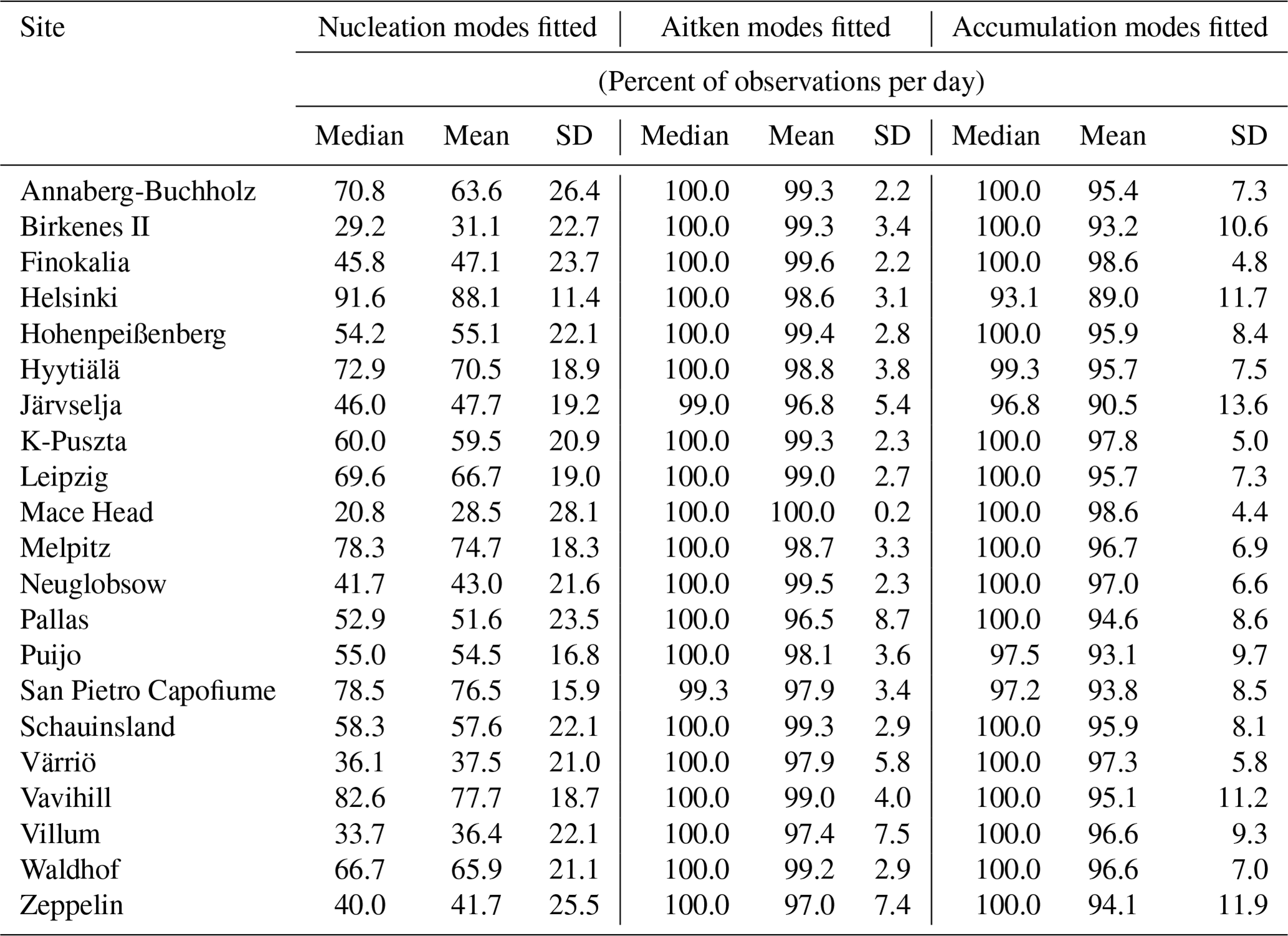
To conclude, the absence of modes did not drastically affect the daily mean of observed modes in Aitken and accumulation modes. As the fraction of fitted nucleation modes is smaller than for Aitken and accumulation modes, results for nucleation mode number concentrations are more uncertain compared to results for the other modes, which should be kept in mind when interpreting the results.
For comparison between climate models and observations, we also computed monthly means (for trend analysis) and seasonal medians (for SeasC – ratio of maximum and minimum of seasonal median values – calculation; see Supplement) of the fitted log-normal modes to the observational data described above. As global model results were monthly means, the same time resolution was also applied for the mode data. Monthly means of the measured data were calculated using the daily averaged data, with the limitation that at least five daily mean values per month were required. This limitation removed only 2 months from the entire data set, in addition to the months that were completely missing from the observational data. Seasonal means and seasonal medians were computed using monthly means with at least two monthly means per season being required.
2.1.3 Remapping measurement data sets for comparison with climate models
As shown later in the results section, the mean diameters of the fitted modes are larger than the corresponding diameters or bins used in climate models. This might affect the model–observation comparison results, especially for the nucleation mode, where the relative difference between the diameters of fitted modes and model modes is largest. Therefore, we calculated separate representations of the measurement data, which are more directly comparable to the model results: for the modal and sectional aerosol schemes, the measurement data were re-binned using the model limits. For comparison, with the Sectional Aerosol module for Large Scale Applications (SALSA), the measured size bins with a mean geometrical diameter of 3 to 7.7 nm were assigned to the nucleation mode. This size range corresponds to the limits of the smallest size bin in a SALSA (Kokkola et al., 2018). Measured size bins from 7.7 to 50 nm (corresponding to the second- and third-smallest size bins in SALSA) were assigned to the Aitken mode and from 50 to 700 nm (fourth- to sixth-smallest size bins in SALSA) to the accumulation mode. In the modal representation for comparison with the modal models, the corresponding size limits were 3 to 10 nm for nucleation, 10 to 100 nm for Aitken, and 100 to 1000 nm for accumulation mode. As can be seen from Table 1, the corresponding diameter range of each mode category from the models is not fully captured by the measurements at every site. If measurements were covering only a part of the model's diameter range, that part has been used as a representative mode from measurements if there are at least three size bins of measurement data available. This limitation was used because the number concentrations from one or two bins have a large variance, resulting in very uncertain trends. If there were fewer bins or no measurement data available, the corresponding nucleation mode is not represented in the results section. For Aitken and accumulation modes, there were always enough data to calculate representative modes, even though the accumulation mode is not always measured up to the diameter of 1000 nm.
2.2 Data from climate models
We used climate model data from EC-Earth3-AerChem (van Noije et al., 2021), the Norwegian Earth System Model NorESM1.2 (Kirkevåg et al., 2018), and the UK's Earth System Model UKESM1 (Sellar et al., 2019), which participated in model simulations carried out within the European-Union-funded project CRESCENDO (Coordinated Research in Earth Systems and Climate: Experiments, Knowledge, Dissemination and Outreach). CRESCENDO simulations ran from the year 2000 to 2014, except for NorESM1.2, which ran from 2001 to 2014. All the models were run in atmosphere-only configuration with sea surface temperatures and sea ice concentrations prescribed as in the Atmospheric Model Intercomparison Project (AMIP) simulation of the Coupled Model Intercomparison Project Phase 6 (CMIP6). The climate models provided monthly values for the aerosol number size distribution, making the data useful for comparison against observations. In addition, we ran two configurations of the global aerosol–chemistry–climate model ECHAM6.3-HAMMOZ2.3-MOZ1.0, one with the M7 modal aerosol model (Tegen et al., 2019) and one with the sectional aerosol model SALSA (Kokkola et al., 2018). Specific features and the aerosol representation of each model are described in the following sections and summarized in Table 3.
Table 3Summary of model set-up, emissions, and aerosol microphysics in five climate models used in this study.
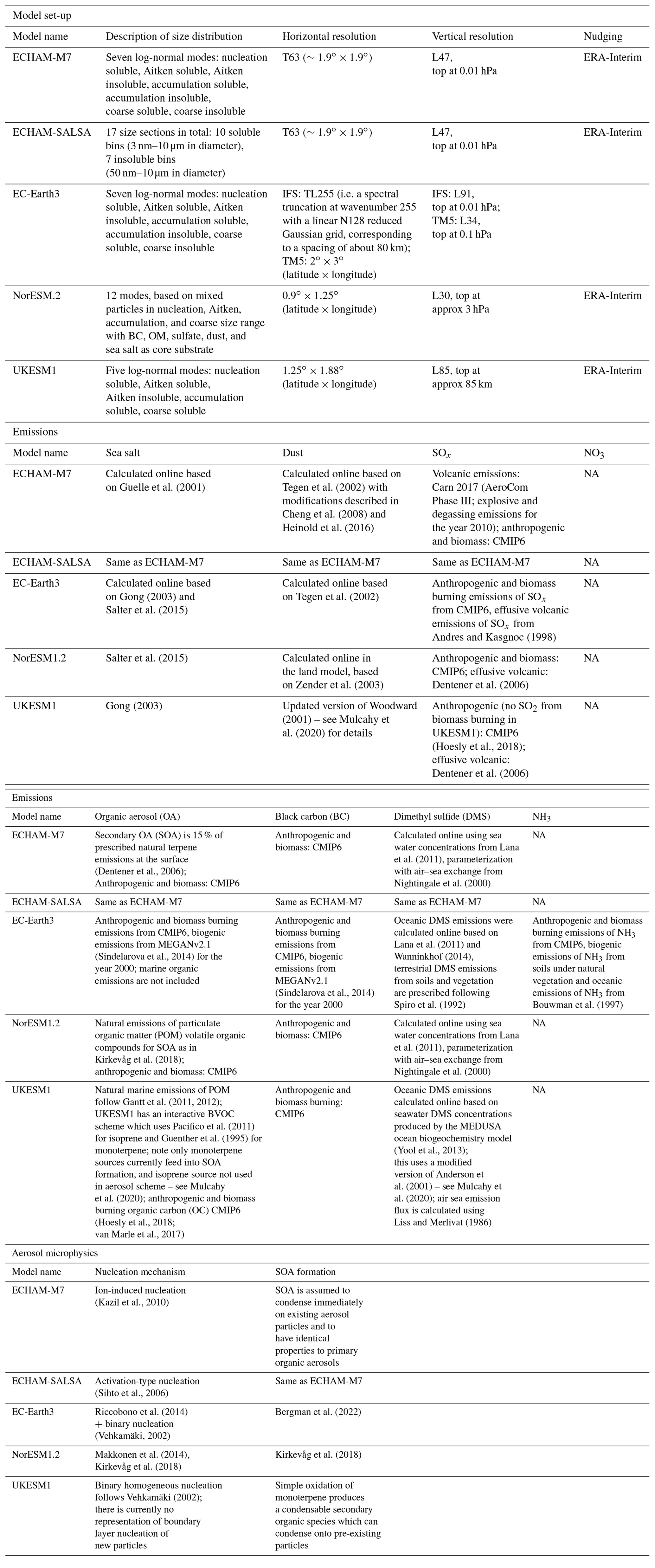
NA: not available.
From the global model calculations, we selected results for grid boxes containing the coordinates of the respective measurement sites and calculated the number concentrations of nucleation, Aitken, and accumulation mode particles. If both soluble and insoluble particle concentrations were provided for the mode, the sum of those has been used as the total number concentration of that mode.
2.2.1 EC-Earth3
The atmospheric component of the global climate model EC-Earth3-AerChem (van Noije et al., 2021) consists of a modified version of the general circulation model used in the Integrated Forecasting System (IFS) cycle 36r4 from the European Centre for Medium-Range Weather Forecasts (ECMWF) and the aerosol and chemistry model TM5. The IFS model version applied in EC-Earth3-AerChem has a horizontal resolution of TL255 (i.e. a spectral truncation at wavenumber 255 with a linear N128 reduced Gaussian grid, corresponding to a spacing of about 80 km) and uses 91 hybrid sigma-pressure levels in the vertical direction with a model top at 0.01 hPa. TM5 uses an atmospheric grid with a reduced resolution of (latitude × longitude) and 34 vertical layers extending to ∼0.1 hPa. The data exchange between the two model components is governed by the OASIS coupler.
The aerosol scheme of TM5 is based on the modal aerosol microphysical scheme M7 from Vignati et al. (2004), which includes sulfate, black carbon, organic aerosols, sea salt, and mineral dust. In TM5, the formation of secondary organic aerosols is described as in Bergman et al. (2022). The concentrations of ammonium, nitrate, and the aerosol water associated with (ammonium) nitrate are calculated assuming equilibrium gas–particle partitioning. In the current model version, this equilibrium is calculated from the Equilibrium Simplified Aerosol Model (EQSAM; Metzger et al., 2002). The chemistry scheme of TM5 accounts for gas-phase, aqueous-phase, and heterogeneous chemistry (van Noije et al., 2021). The sources of mineral dust and sea salt, the oceanic source of DMS, and the production of nitrogen oxides by lightning are calculated online. Emissions from anthropogenic activities and open biomass burning are prescribed using data sets provided by CMIP6. All other emissions are prescribed as documented in van Noije et al. (2021).
2.2.2 ECHAM-HAMMOZ
ECHAM-HAMMOZ (echam6.3-hammoz2.3-moz1.0) is a global aerosol–chemistry–climate model which consists of the atmospheric circulation model ECHAM (Stevens et al., 2013), the aerosol model HAM (Kokkola et al., 2018; Tegen et al., 2019), and the chemistry model MOZ (Schultz et al., 2018) not used in this study. The model solves atmospheric circulation in three dimensions with spectral truncation of T63, which corresponds to approximately horizontal resolution and uses 47 vertical layers extending to 0.01 hPa. The model includes the sectional aerosol model SALSA, which describes size distributions using 10 size bins between 3 nm and 10 µm in diameter, with externally mixed parallel size bins between 50 nm and 10 µm for treatment of particles consisting of insoluble material when they are emitted. The ECHAM-HAMMOZ also includes an option of using the modal aerosol model M7, which describes the aerosol size distribution with a superposition of seven log-normal modes. Details of how aerosol processes are calculated in SALSA are described by Kokkola et al. (2018). The same details for M7 are described by Tegen et al. (2019).
Both model configurations (i.e. SALSA and M7) were set up according to the AeroCom (Aerosol Comparisons between Observations and Models) initiative phase III experiment set-up. Anthropogenic aerosol emissions were according to the Community Emissions Data System (CEDS; Hoesly et al., 2018); for biomass burning, we used Biomass Burning Emissions for CMIP6 (BB4CMIP; van Marle et al., 2017). Dust, sea salt, and maritime DMS emissions are calculated online as a function of 10 m wind speed (see Tegen et al., 2019, and references therein). Atmospheric circulation (vorticity, divergence, and surface pressure) was nudged towards ERA-Interim reanalysis data (Berrisford et al., 2011), but temperature was allowed to evolve freely.
2.2.3 NorESM1.2
NorESM1.2 (Kirkevåg et al., 2018) is an earth system model which consists of the atmospheric model CAM5.3-Oslo, the sea ice model CICE4, the land model CLM4.5, and an updated version of the MICOM ocean model used in NorESM1 (Bentsen et al., 2013). CAM5.3-Oslo is based on CAM5.3 (Liu et al., 2016; Neale et al., 2012) but contains a different aerosol scheme (OsloAero5.3), along with other small modifications. In this study, the model is run with a horizontal resolution of and 30 layers in the vertical (model top at around 3 hPa).
The aerosol scheme in NorESM1.2 describes aerosols using 12 separate modes, which can consist of sulfate, BC, OM (including SOA), sea salt, or dust (see Kirkevåg et al., 2018, for a detailed description), and their interaction with radiation and clouds. Emission strength of natural aerosol precursors and aerosols such as dust, sea salt, primary marine organic matter, marine DMS, isoprene, and monoterpenes is calculated interactively (Kirkevåg et al., 2018). The nucleation scheme for new particle formation used in NorESM1.2 is described in Makkonen et al. (2014). We have used the anthropogenic emissions from Hoesly et al. (2018) and biomass burning emissions from van Marle et al. (2017). We prescribed sea-surface temperatures and sea ice concentrations based on observations, and in the atmosphere, the horizontal wind (the zonal wind speed U and the meridional wind speed V) and surface pressures were nudged to 6-hourly ERA-Interim reanalysis data.
2.2.4 UKESM1
The United Kingdom Earth System Model (UKESM1) is described in detail by Sellar et al. (2019) and is built around the Global Coupled 3.1 (GC3.1) configuration of the HadGEM3 (Hadley Centre Global Environment Model) physical climate model (Kuhlbrodt et al., 2018; Williams et al., 2018). UKESM1 additionally includes ocean and land biogeochemical processes and a stratospheric–tropospheric chemistry scheme (Archibald et al., 2020) implemented as part of the United Kingdom Chemistry and Aerosol (UKCA) model. In the simulations performed for the CRESCENDO project, UKESM1 was set to operate at a horizontal resolution of (latitude × longitude), with 85 vertical levels.
The representation of aerosols within UKESM1 is described and evaluated by Mulcahy et al. (2020); UKESM1 employs the modal version of the Global Model of Aerosol Processes (GLOMAP) two-moment aerosol microphysics scheme (Mann et al., 2010). The aerosol number size distribution is represented by soluble nucleation, Aitken, accumulation, and coarse (diameter >1000 nm) modes and an additional insoluble Aitken mode. The above modes are used to carry information about sulfate, black carbon, particulate organic matter, and sea salt, whilst mineral dust is treated using the separate sectional scheme of Woodward (2001). In UKESM1, there is no parameterized new particle formation scheme applied in the boundary layer.
Anthropogenic emissions of aerosols are prescribed from the CMIP6 inventories: SO2 and anthropogenic BC and OC are taken from the Community Emissions Data System (CEDS; Hoesly et al., 2018), and biomass burning emissions are from van Marle et al. (2017). UKESM1 interactively simulates emissions of marine DMS, biogenic volatile organic compounds (BVOCs), and primary marine organic aerosol (Sellar et al., 2019).
2.3 Data analysis methods
2.3.1 Observational short-term trends: dynamic linear model (DLM)
We used the dynamic linear model (DLM) for determining the short-term variation in trends, i.e. transient changes in the (long-term) trend in timescales of some months to some years, of different measured mode parameters in the daily data set (Durbin and Koopman, 2012; Laine, 2020; Petris et al., 2009). The main advantage of DLM compared to many other non-parametric and parametric trend estimation methods is that DLM can also detect a non-monotonic trend, and the seasonality of the time series can be estimated simultaneously with the trend.
DLM explains the measured variability in the time series yt of the mode parameter (N, Dp, or σ) with three components: firstly, the level component μt that is locally linear, but the trend αt can change during the measured period; secondly, a seasonality component γt that captures the seasonal pattern of the time series; thirdly, a residual component ηt that uses an autoregressive model (AR(1), ρ) and accounts for autoregression of the time series, i.e. dependence of the daily measurement on that from its previous day; and finally normally distributed random noise components εt, εlevel,t, , and εAR,t, which are related to uncertainties in each component. For each observation yt at time t the DLM model used in this study is given by
where , , , , and . We have used ρ=0.4 as a value for AR(1) coefficient in all model fittings. The initial value of the level has been set to be the yearly mean of the first year. Calculation of the DLM model has been done in the MATLAB environment (MATLAB, 2019) using the DLM MATLAB Toolbox (Laine et al., 2014).
As the applied DLM formulation assumes normally distributed data, we used log10 transformation for mode number concentrations. If number concentration was zero (i.e. no fitted modes were available for that day), we used a value of one as a number concentration for that day to avoid problems with log10 transformation. For mode diameter and geometric standard deviation, no transformations were applied. We investigated the residuals εt after the model fitting, and in most cases, the assumptions of the model are sufficiently fulfilled, with the distribution of the residuals being close to a normal distribution. Before interpreting the level and the trend of the number concentration of each mode, we have transformed the level μt and trend αt back to the original scale by using the exponential back-transformation.
2.3.2 Long-term linear trends: Sen–Theil estimator
Long-term trends of measured mode parameters in the data set were estimated using the Sen–Theil estimator (Sen, 1968; Theil, 1950). The Sen–Theil estimator is a non-parametric method to estimate a linear trend. The advantages of the Sen–Theil estimator compared to more common linear regression methods are that it does not assume normality of the data, and it is more robust to outliers. Compared to the more complex DLM model, the Sen–Theil estimator also works with a lower number of data points, which is one reason we used it in the model comparison.
Trend estimation was performed using the TheilSen function from openair package in the R environment (Carslaw and Ropkins, 2012; R Core Team, 2021). The calculation of 95 % confidence intervals is based on the bootstrap method (Kunsch, 1989). Trend estimation was done for whole-year data (monthly averages) and seasonal data (monthly averages of a specific season). Before trend estimation for the whole-year data set, the time series was de-seasonalized with seasonal trend decomposition using loess, and autocorrelation for consecutive months was taken into account when calculating the uncertainty in the trend estimates. Seasons have been defined to be 3 months each, winter consisting of December–February, spring March–May, summer June–August, and autumn September–November. In the trend estimation for observational data sets (Sect. 3.1), we have used all months available from each site. In all comparisons of observations and models (Sect. 3.2), we used only those months that were available from the measurement sites.
We have used relative change (% yr−1) as the main parameter for comparing results. Relative change has been calculated for the Sen–Theil estimator and confidence intervals by using the option slope-percent. The function uses the fitted value of a first observation as a reference for calculating relative change (Carslaw and Ropkins, 2012).
2.3.3 Magnitude and pattern of seasonality
The seasonality of particle number concentration and its magnitude is highly varying between different measurement sites, depending on, for example, latitude and environment type of site (Asmi et al., 2013; Rose et al., 2021) and the mode studied. Similarly, parameters such as cloud condensation nuclei (CCN) number concentrations and new particle formation (NPF) frequency have a seasonal cycle (Asmi et al., 2011; Nieminen et al., 2018). Seasonality of the optical properties in models has been studied (Gliß et al., 2021), but for particle number concentrations we are not aware of studies that compare measurements and models based on long-term data sets.
We compared the seasonality of number concentrations in models and measurements by studying modes separately. We used two variables, the normalized interquartile range (NIQR) and SeasC (Rose et al., 2021), to compare seasonality between models and measurements. When calculating these seasonal parameters from measurements and model results, we included only those months for which the measurement and model data were available. We calculated NIQR and SeasC separately for each year to also assess the distribution of values in the studied period.
NIQR, defined as NIQR , describes the interquartile range of observations for 1 year. NIQR was calculated using monthly averages of concentrations, with at least 10 monthly averages needed to be available. The calculation of NIQR is slightly different from Rose et al. (2021), who used daily values calculating NIQR. As we had only monthly averages from model data, daily values could not be used. Based on the measurement data, we checked whether the time resolution would change the NIQR values, by comparing NIQR values calculated from daily and monthly averages. We found that the NIQR values calculated from daily averages were usually higher, sometimes as much as twice the one calculated from monthly averages. Therefore, NIQR values presented in this study are not comparable to values presented in Rose et al. (2021) but only between the different data sets in this study or others calculated from monthly averages.
SeasC is the ratio of maximum and minimum of seasonal median values, calculated separately for each year and mode in each data set. It was calculated by first taking the seasonal averages for each season. For calculating the seasonal median, at least two monthly means from the season were required. Then, if we were able to calculate all the seasonal medians for the year, SeasC was calculated as the ratio of the maximum and minimum of those seasonal medians.
In general, both SeasC and NIQR describe the distribution of number concentrations within 1 year. SeasC focusses more on utmost values, minimum and maximum of seasonal medians, whereas NIQR focusses on values closer to the yearly median. Neither SeasC nor NIQR considers when the maximum and minimum in number concentrations are achieved. Though the seasonal cycle of the measured and modelled number concentrations might be opposite to each other, the difference in SeasC or NIQR values can be small when comparing measurements and model data.
To assess whether the seasonal maximums and minimums have similarities between measurements and models, we have calculated the seasonal averages, selected the seasons that have most often had seasonal maximum and minimum during the measured time period, and evaluated how modelled results correspond to the measurements.
3.1 Observational number size distribution characteristics and trends in daily in situ measurement data sets
We investigated the mode characteristics (number concentration N, geometric mean diameter Dp, and geometric standard deviation σ) for nucleation, Aitken, and accumulation modes for 21 European and Arctic sites representing Polar (Villum, Zeppelin), arctic remote (Pallas, Värriö), rural (Birkenes II, Hohenpeißenberg, Hyytiälä, Järvselja, Melpitz, San Pietro Capofiume), rural regional background (K-Puszta, Neuglobsow, Waldhof, Vavihill), urban (Annaberg-Buchholz, Helsinki, Leipzig, Puijo), coastal remote (Mace Head, Finokalia), and high-altitude (Schauinsland) environments. Median values and interquartile ranges for different mode parameters for the sites over the analysis period are shown in Fig. 1 (and for different seasons in Figs. S4–S6). Figure 1 shows a large variation in N's between the sites. As expected, the Arctic and other remote sites had the lowest concentrations overall (median concentrations 10–150 cm−3 for nucleation and 40–1400 cm−3 for Aitken mode), while urban sites and central European sites had the highest concentrations, especially for the nucleation and Aitken modes (400–2000 cm−3 for nucleation and 800–3600 cm−3 for Aitken mode). Generally, N values were higher for southern compared to northern sites. Partially the differences between southern and northern sites could be explained by the relation between population density and station location: more polluted site types were typically found in the south. However, the concentrations for southern sites were higher also within site classes. For the accumulation mode, the highest N values were found at more polluted rural sites in central Europe, K-Puszta and San Pietro Capofiume. These results are in line with previous results for number concentrations, such as those found by Rose et al. (2021).

Figure 1Summary of mode parameters (number concentration N, geometric mean diameter Dp, and geometric standard deviation σ) for the measurement sites. The median values are marked with dots and interquartile ranges (25 % and 75 %) with whiskers for different mode parameters in fitted modes.
For modal Dp and σ, results were not as distinctive for different environments. Standard deviations σ were highest for nucleation modes and lowest for accumulation modes without clear differences between site environmental types. This was kind of expected based on the earlier results showing the relationship between aerosol variability and size (Williams et al., 2002).
Coastal sites Finokalia and Mace Head showed the largest modal Dp in Aitken and accumulation modes, while Birkenes II (rural) and Mace Head showed the largest modal Dp in nucleation mode. Järvselja (rural) had the lowest modal Dp in all modes. One aspect that could explain some of the differences in modal Dp between sites is the lower limit of the detected size range in the measurements. The lower value of the smallest detectable size might increase the probability that the modal Dp of fitted nucleation mode is smaller. For example, for the Mace Head site the lowest measured size bin is around 21 nm, affecting the modal Dp of the fitted nucleation mode. The lowest detected size may also affect the fitted Aitken mode diameter. However, for Finokalia and Järvselja, the measured size range could not completely explain observed high and low modal Dp of the nucleation, respectively. This was tested by using a minimum size of ∼10 nm for those sites that have measured <10 nm particles and calculating the mode parameters as in Fig. 1. For this test, modal Dp was calculated using ∼10 nm, as the lowest size in Finokalia was close to diameters using the original lowest size in Fig. 1. Geometric mean diameters in Järvselja increased by some nanometres but were still lowest among all sites, except in nucleation mode, where Villum then had the lowest modal Dp.
To investigate the effect of measurement size range on mode fitting, we studied the dependence of modal Dp and minimum size bin measured amongst all sites. Spearman's rank correlation between modal Dp and the lowest size bin amongst sites was positive, 0.67 for nucleation, 0.03 for Aitken, and 0.26 for accumulation mode, indicating the strongest dependence for nucleation modes and only a minor dependence for accumulation modes. Thus, especially for nucleation modes, the lowest detectable size is related to the lower modal Dp in Fig. 1.
Results for modal Dp are somewhat different compared to what has been observed in Rose et al. (2021). Rose et al. (2021) used a slightly different site classification than that employed in this study. Unlike the classification used in our study, they classified the stations based on both geographic area (e.g. mountain and continental site classes) and footprint (e.g. urban and rural site classes). In their study, one site could have belonged to more than one site class. Hence, even if there are the same sites used in Rose et al. (2021) and our study, the classification was different. With their classification, they reported that mode diameters for Aitken and accumulation modes were smallest for urban sites (32±11 and 122±37 nm; Leipzig in our study), followed by mountain (39±9 and 142±25; Hohenpeißenberg), polar (42±14 and 149±37; Pallas, Värriö, and Zeppelin), and continental (51±13 and 174±29; Annaberg-Buchholz, Birkenes II, Hyytiälä, K-Puszta, Leipzig, Melpitz, Neuglobsow, Schauinsland, Vavihill, and Waldhof) sites. (The sites used in both studies are mentioned in the brackets.) In our results, most urban sites had a smaller Aitken mode modal Dp compared to most of the rural continental sites, with the most notable exceptions from this tendency being Puijo and Järvselja. Otherwise, the differences between site types reported by Rose et al. (2021) were not observed in our study. In general, the modal Dp values were smaller in our study; however, the rural sites in our study and continental sites in Rose et al. (2021) have accumulation mode diameters close to each other. Rose et al. (2021) studied only particles ranging from 20 to 500 nm and the year 2016 or 2017, depending on the site. They also had a larger number of sites considered. In our analysis, the analysed particle size range has in particular affected the mean diameters since at least part of the 20–30 nm particles were fitted into nucleation mode, whereas in Rose et al. (2021), those were included in the Aitken mode. As a result, the fitted Aitken modes in our study had slightly larger modal Dp compared to fitting only Aitken and accumulation mode.
It is worth noting that the fitted modes and their diameters were mostly larger than what is usually assumed in climate models. Fitted nucleation modes had mean diameters from above 10 nm (Järvselja) to around 20 nm (Mace Head), while the upper limit of the nucleation mode in sectional (7 nm) and modal (10 nm) model representations is below all the medians of fitted mean diameters to the observational data. Higher nucleation mode mean diameter detected in the measurements may be due to the fact that the lowest detectable diameter is usually around the upper limit of model representations. As the measurements do not capture the smallest nucleated particles and only detect them after some growth, the average nucleation mode diameters determined from measurements may be an overestimation.
To investigate the short-term trends at different measurement sites over the analysed time periods, we used DLM analysis as described in Sect. 2.3.1. To demonstrate the characteristics of a DLM trend fit, Aitken mode N's and their estimated level for the Mace Head site are shown in Fig. 2. Aitken mode N's at Mace Head were selected as an example because there is a substantially large increase in number concentration during the measured period, which is also seen in Fig. 3, showing the estimated trend in Aitken mode for all sites. The trend at Mace Head given by DLM (red line in Fig. 2) was temporarily over 10 % yr−1. It must be noted that the concentrations at Mace Head were quite low compared to many other sites, and the variation in average N in Aitken modes between days was relatively large, ranging from 50 to 3000 particles cm−3. The number of high-concentration days (here denoted as >500 particles cm−3 on average) increased towards the year 2010 and has been decreasing since then. In the year 2010, the frequency of high-concentration days was about 68 % of the days observed, while in 2005–2008 it was about 46 %. In the year 2012, the frequency of high-concentration days was increased to 51 %. For Mace Head, the Aitken mode Dp had an opposite but a much weaker trend: there was an increasing trend in diameter before the year 2008 and a decreasing trend from 2008 to 2010, and after that, the trend was increasing again. Based on this data set, we cannot derive the exact reasons for the changing N.
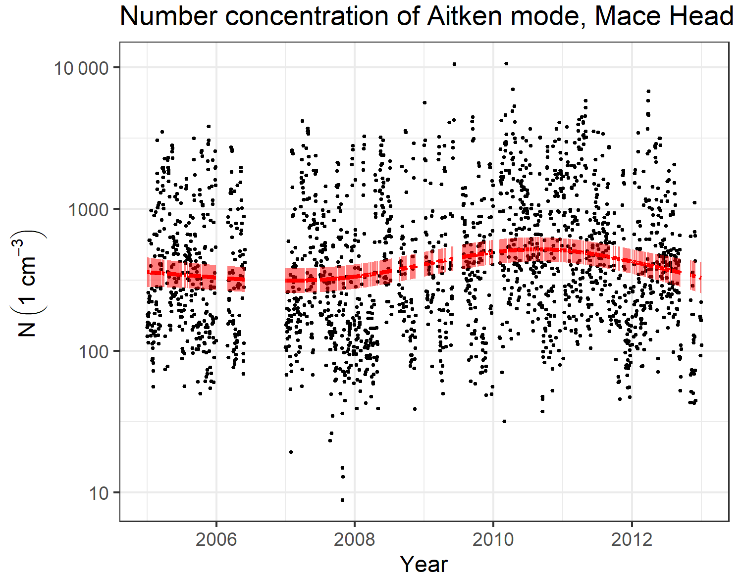
Figure 2DLM fit for Mace Head Aitken mode number concentration. Black dots represent daily averages of Aitken mode number concentrations at Mace Head. The solid red line represents the estimated level, and the red ribbon represents the 95 % confidence interval for the level.
In Fig. 3. we present the coefficients for the DLM trend for Aitken mode Dp and N. Mode parameters Dp and N were selected because those parameters show the strongest trends. Results for nucleation and accumulation modes are shown in Figs. S7 and S8. The trend derived using the DLM showed the transient changes in the level of the time series. The trend from the DLM was constantly changing during the time series, achieving the best fit to the data as can be seen in Fig. 3. For Fig. 3, the unit of the change was scaled to be comparable with the long-term trends presented later. To get a DLM trend for 1 year, the 1 d trend given by the model was multiplied by the number of days in a year (365 used for all years) and divided by the mean of the variable over the first observed year.
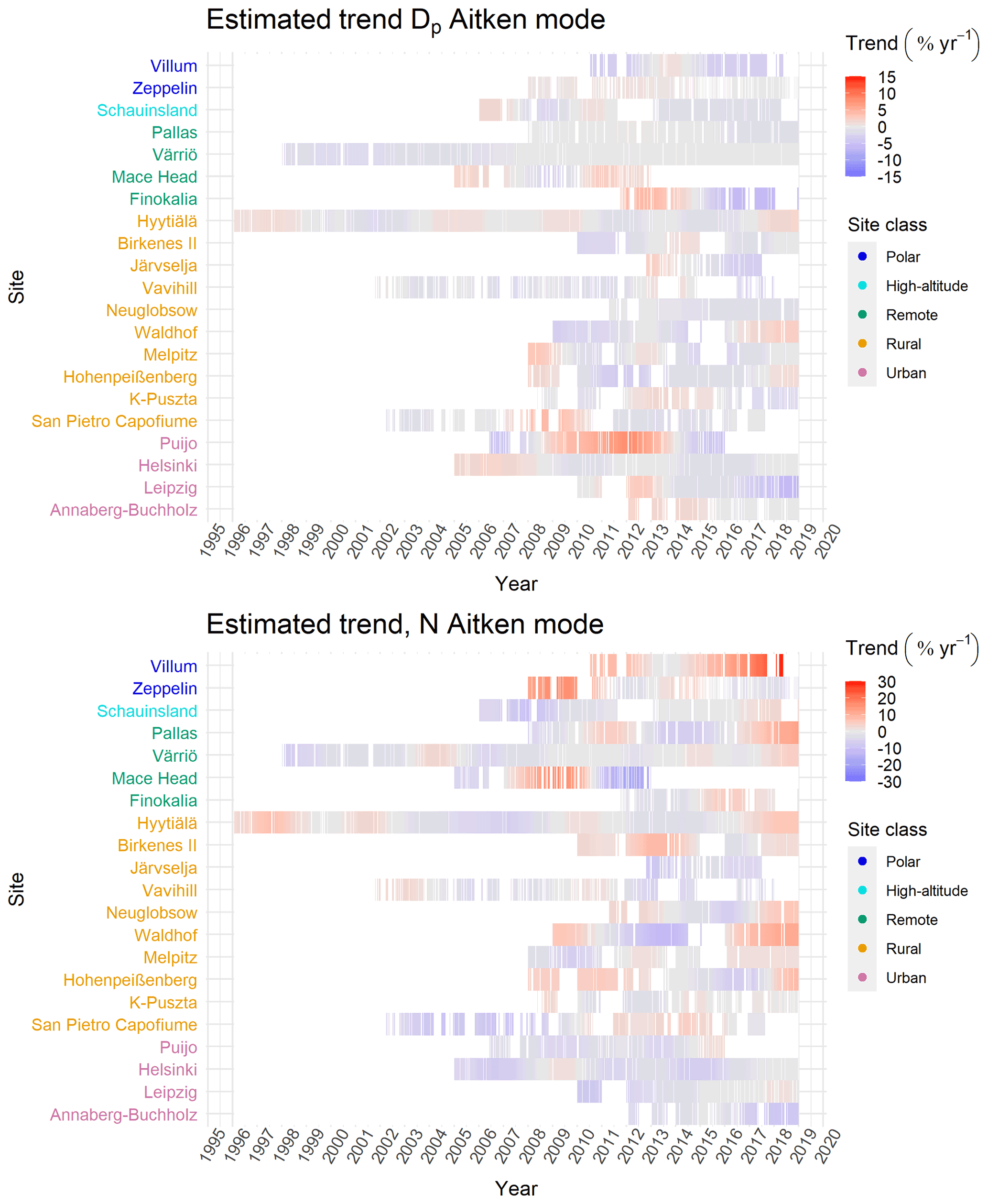
Figure 3Estimated trends for Aitken mode Dp and N at measurement sites. Trend has been calculated by DLM; see Sect. 2.3.1 for details. The overall trend presented in the figure is comparable with the long-term trend estimates given in Sect. 3.1. To get a DLM trend for 1 year, the 1 d trend given by the model was multiplied by the number of days in a year (365 used for all years) and divided by the mean of the variable over the first observed year. For example, if the trend shows an increase of 10 % yr−1 it means that if the short-term increase would continue for a year, the concentration would be increased by 10 % during the year compared to the first-year mean.
The most important result of the DLM analysis was that the trends are usually not monotonic during the measured period. Therefore, long-term trends should be only thought of as an approximation of the average change during the time period. It is also good to note that the mode parameters are connected; i.e. for some of the short-term trends observed in mode number concentration, there was an opposite trend in mode mean diameter. This can also be seen later in the long-term trends (Sen–Theil results) for some of the modes and sites.
The long-term trends were investigated using Sen–Theil estimators (Fig. 4). Exact numbers for trends and confidence intervals are shown in Fig. S9. Number concentration N of the modes showed the largest changes over the investigated time periods, modal Dp has the second-largest changes, and σ showed only minor variations compared to the other two parameters. This was similar for both the Sen–Theil estimator and DLM results.

Figure 4Long-term trend estimators for measured trends of all mode parameters (mean geometric diameter Dp, geometric standard deviation σ, and number concentration N) in nucleation (NuclM), Aitken (AitM), and accumulation mode (AccM). Confidence intervals (95 % confidence level) are shown with whiskers. Trends have been calculated using the Sen–Theil estimator and complemented with bootstrap confidence intervals (see Sect. 2.3.2).
Amongst all variables and sites considered, accumulation mode N showed the largest decrease, followed by Aitken and nucleation mode N when long-term trends are considered (Fig. 4). Only urban sites showed consistent decreases in number concentration for almost all modes and sites. The only exception here is semi-urban Puijo, which showed an increasing trend in accumulation mode N. Urban sites are dominated by anthropogenic emissions (e.g. traffic and industrial activities), which are affected by recent air quality control measures in Europe. This naturally explains the decreasing trends at urban sites, as discussed in previous studies (Mikkonen et al., 2020; Sun et al., 2020). For rural and remote sites, there was more site-to-site variation in trends, and some of these sites showed trends of increasing N in all three modes. The rural and remote sites are less directly affected by anthropogenic sources, but more by biogenic or other natural sources compared to urban sites. The strength of the anthropogenic contribution varies between the rural and remote sites depending on the strength of the natural sources and transportation efficiency of air masses from more polluted environments. For example, the central and southern European rural sites are likely more affected by anthropogenic sources than northern European rural or remote sites due to denser incidence of large urban areas in central and southern Europe. The biogenic emissions depend greatly on environmental factors, which can vary significantly on a year-to-year basis and between sites. In case of accumulation mode there can also be differences in removal efficiency linked to differences in cloud cover and precipitation at different sites. These factors may partly explain the large variation in trends between the different rural or remote sites. The difference in trends of N in the three modes at the same site may be related to different sources and their temporal changes. Furthermore, nucleation and Aitken mode particles are likely to be emitted or formed close to the measurement site, while accumulation mode particles are often transported to the location over longer distances. In particular, nucleation mode N values are dependent on the formation of particles and their growth to larger sizes, which in turn are dependent on not only the precursor gas emissions but also meteorological conditions and background particle concentrations (Nieminen et al., 2018). Thus, a decreasing trend in the concentration of larger particles could even strengthen new particle formation.
Mace Head showed distinctly different behaviour compared to other sites as the number concentration of all three modes had increasing annual (Fig. 4) and seasonal trends (Fig. 5). It should be noted here that the investigated period of the Mace Head data set differs considerably from other investigated data sets: for Mace Head, the investigated period ends in the year 2012, while for other sites the time period ends in 2017 or 2018.
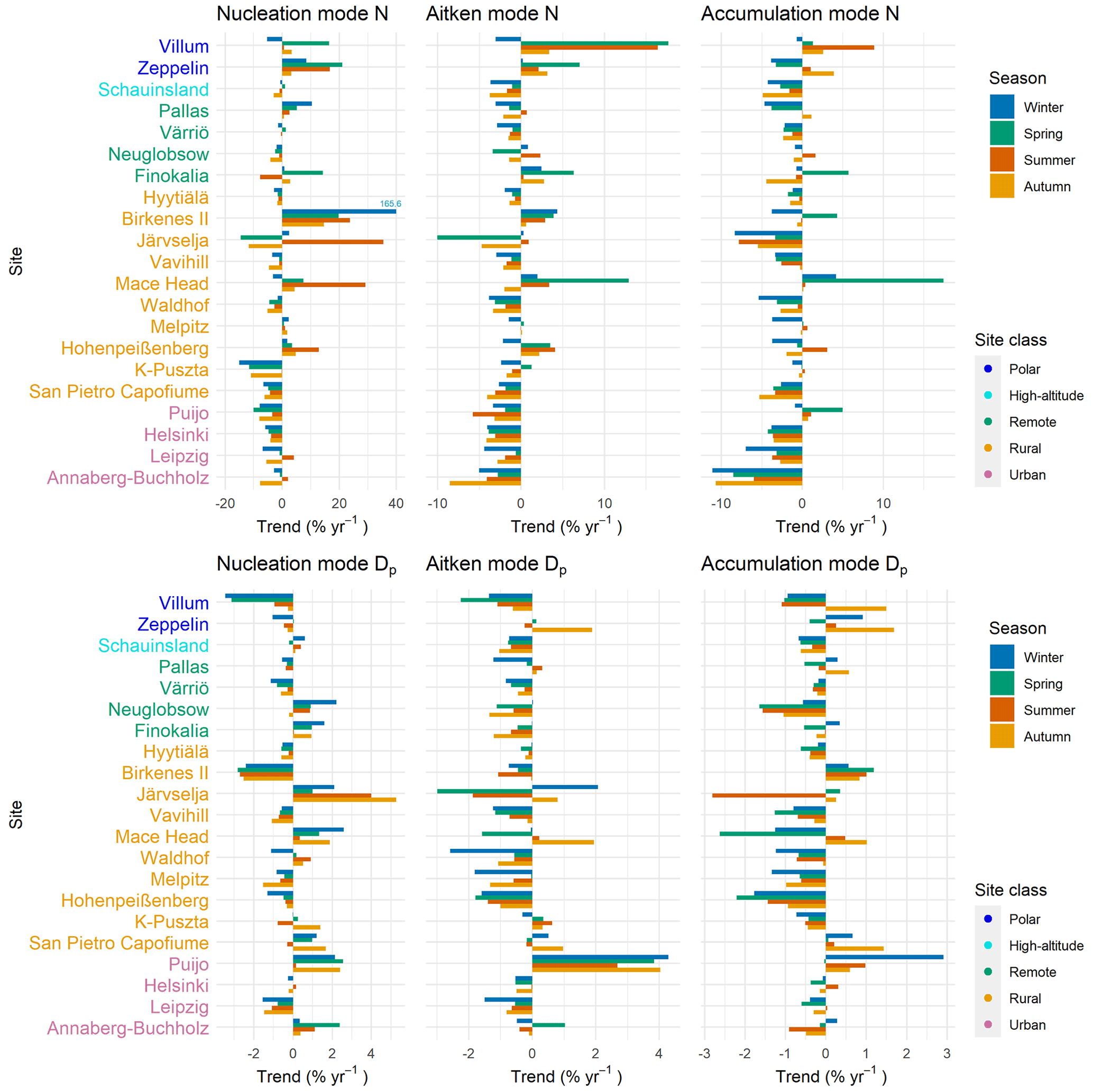
Figure 5Seasonal long-term trend estimates for all mode parameters: mean geometric diameter Dp, geometric standard deviation σ, and number concentration N in nucleation (NuclM), Aitken (AitM), and accumulation mode (AccM) during autumn (September, October, and November), winter (January, February, and December), spring (March, April, and May), and summer (June, July, and August). Trends have been calculated using the Sen–Theil estimator and complemented with bootstrap confidence intervals (see Sect. 2.3.2). Correct number for nucleation mode N trend for Birkenes II is shown next to the bar.
Accumulation mode correlation between the estimated trend coefficients for modal Dp and N was −0.27. So, the decrease in number concentration was somewhat concurrent with increased particle size in accumulation mode (see also Fig. S10). For the σ parameter, the trend was almost zero for most of the sites.
For the Aitken mode and especially the nucleation modes, there were some sites that show an increase in N. For the Aitken mode, the Spearman correlation between trend estimates of modal Dp and N was −0.25, and for nucleation mode, the spearman correlation was −0.47. Thus, especially in nucleation mode, some of the increases and decreases in number concentration were partially connected with a decrease or increase in modal Dp (see also Fig. S10). Additionally, in nucleation and Aitken modes, the σ parameter showed only minor changes during the measured period.
We also investigated if the trends have a seasonal behaviour. For seasonal trends in general, a decrease in N was strongest for winter and weakest for summer (Fig. 5, exact numbers in Figs. S11 and S12). In winter, there were relatively consistent decreasing trends all over Europe. In autumn (Figs. 5 and S11), the trends were also mostly decreasing. In summer and spring (Figs. 5, S11, and S12), there were clear differences in trends between sites. Again, the most consistent trends were at urban sites, showing a decrease for accumulation and Aitken mode N. Nucleation mode N for urban sites also mostly decreased. Other site classes did not show consistent decreases, possibly due to different contributions of anthropogenic and biogenic emissions between sites, as previously discussed in this section. Large, sporadic, increasing trends in nucleation mode might have resulted from a large portion of missing nucleation modes fitted and small concentrations, which might cause large trends even for small absolute changes. During the winter season (Figs. 5 and S11), this results in a stronger, decreasing trend in wintertime concentrations compared to summertime trends. This was most evident for accumulation and Aitken mode particles. Interestingly, especially during winter seasons, the nucleation mode exhibits an opposite observed trend to the accumulation and Aitken mode concentrations (Figs. 5 and S11). As noted earlier, different trends in nucleation mode number concentrations than for larger particles might be related to different sources and the effect of background particles on new particle formation acting as a condensation sink.
3.2 Comparison of observed particle mode concentrations and climate model results
In this section, we compare the observational trends of N of each mode to the trends of the climate model simulation data. These results are not fully comparable to the results presented in Sect. 3.1 since the investigated time period in this section is different from the time period in Sect. 3.1. For comparison of simulations and observations, at least 7 years of data were required. Because model data were only available for the years 2001 through 2014, this limited the number of sites available for the comparison. Figures 6–8 display the 13 sites that had sufficient data coverage for this time period. In the cases where measurement data were missing for a site for a certain month, model data for the corresponding month were omitted as well. As explained in Sect. 2.1.4, log-normal modes that were fitted to the measurement data were not directly comparable to the data provided by the climate models. We therefore additionally remapped the size distributions for specific size intervals (see Sect. 2.1.4) which were used in the models from the measurement data to correspond to the sectional (ECHAM-SALSA) and modal (EC-Earth3, ECHAM-M7, NorESM1.2, and UKESM1) representations of nucleation, Aitken, and accumulation mode as used in the models. To this end, we used the model-internal parameters to separate the respective modes (see Sect. 2.1.4 for details). In the following, we thus analyse three representations of the same measurement data, which we refer to as “fitted modes” (Sect. 2.1.3) and “sectional” and “modal representation of the measurement data” (Sect. 2.1.4). While these three representations were not directly comparable to each other (because the size ranges for different modes varied between the different representations), it was still instructive to visualize them side by side. It should also be noted that the trends for the fitted modes in Figs. 6–8 were not the same as in Fig. 4 because the time intervals of the trend analyses were not the same.
3.2.1 Comparison of yearly trends
Figure 6 shows the trends in nucleation mode N; exact numbers for trends are shown in Fig. S13. Unfortunately, at many measurement sites, the minimum detected particle diameter was too large to compute meaningful results for nucleation-mode-sized particles that were comparable to the models. Hence only five of the measurement sites (Hyytiälä, Helsinki, Vavihill, Melpitz, San Pietro Capofiume) could be compared to all models, and three additional sites (K-Puszta, Pallas, Värriö) could be compared to models with modal aerosol representation. Of these sites, Hyytiälä, Helsinki, Vavihill, and San Pietro Capofiume showed comparable trends for all three representations of the measurement data, which were all decreasing and statistically significant. At all four of these measurement sites, the models showed decreasing trends as well, but in many cases, the negative trends were weaker, and sometimes no significant trend was found. Observations at Pallas showed a strong increasing trend for both fitted mode and modal representation of the data, while all models showed slightly decreasing trends, of which one result was statistically significant.
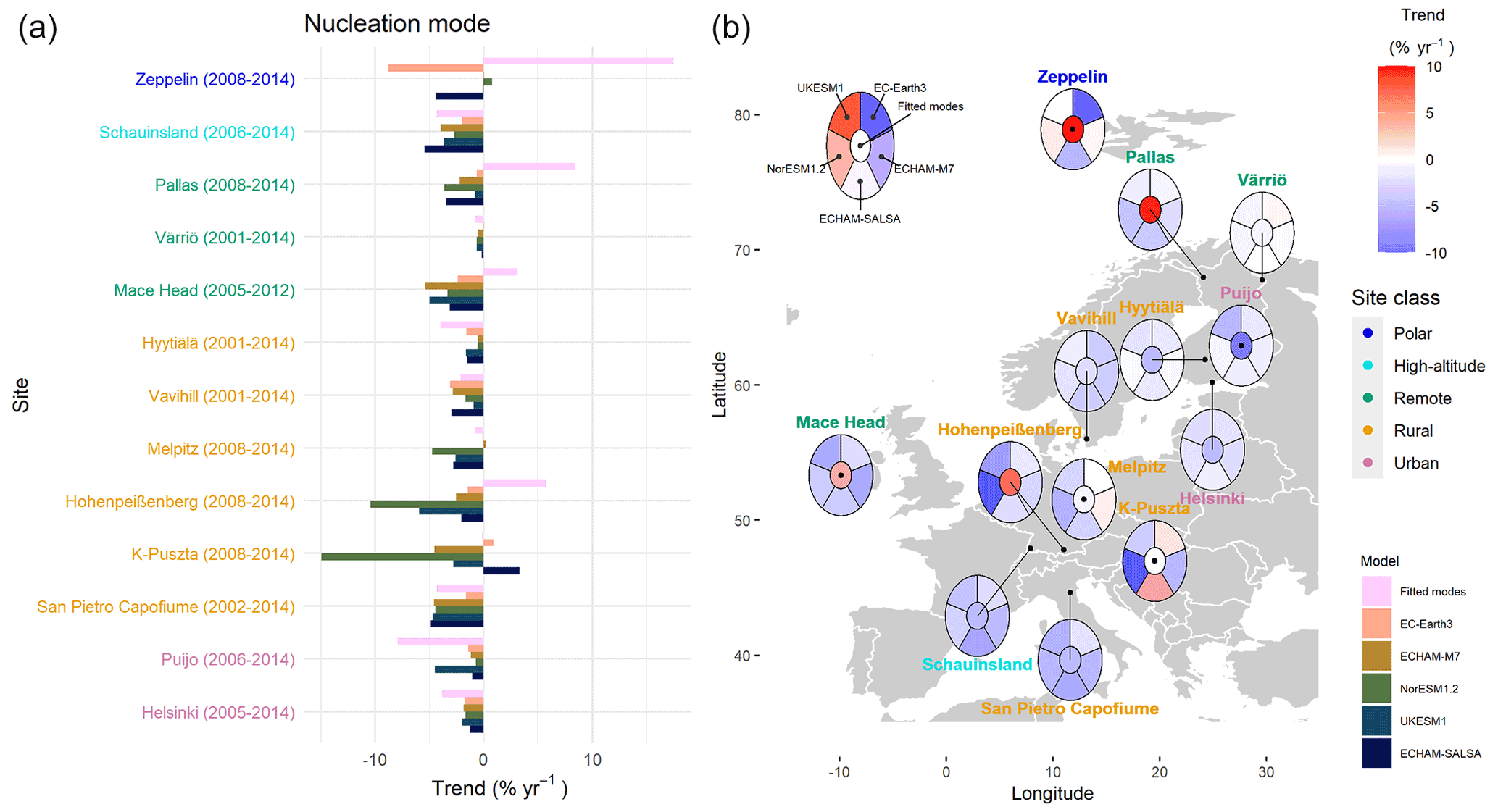
Figure 6Long-term trend estimates for measured and modelled nucleation mode number concentration. (a) Bar plot of trends for different sites. The sites (y axis) are arranged by site class and within site class most northerly to most southerly. (b) Estimated trends presented on the map. The colour of the central part follows the trend of the fitted modes. Trends have been calculated using the Sen–Theil estimator and complemented with bootstrap confidence intervals (see Sect. 2.3.2).
When inter-comparing model results, we found that for most sites all models showed slight to medium decreasing trends (about 0 % to −5 % yr−1) for nucleation mode N (Figs. 6 and S13). This was also expected, as all models used the same anthropogenic emission inventory, which exhibits a steadily decreasing trend in sulfur dioxide emissions over Europe for the modelled period (Hoesly et al., 2018). This directly affects nucleation rates and condensation rates of sulfuric acid in the models. There were only two measurement sites that deviate from this general model trend. At K-Puszta, EC-Earth3 and ECHAM-SALSA showed increasing trends for the nucleation mode concentration. The other exception was a very strong decreasing trend in nucleation mode particle concentration for K-Puszta and Hohenpeißenberg in NorESM1.2. For both sites, however, the accumulation mode showed a positive trend in NorESM1.2, which was not present for the other models. A growing number of accumulation mode particles probably led to a larger condensation sink and therefore to suppression of new particle formation in the model.
Figure 7 shows the yearly trends in Aitken mode N; exact numbers for trends are shown in Fig. S13. When the three representations of observations were investigated it can be concluded that the three different representations of the measurement data qualitatively agreed at most sites. The only exceptions were Pallas, where trends varied between −0.7 % (fitted mode) and +3.1 % yr−1 (sectional representation), and for Zeppelin, where the positive trend was stronger in the sectional representation compared to the other two representations (Fig. S13). Furthermore, except for Zeppelin, Pallas, Mace Head, and Melpitz, all observational trends for all three representations were statistically significant. Of all statistically significant trends, only Hohenpeißenberg showed a positive trend in Aitken mode N for all three observational representations. Mace Head and Zeppelin were quite different, as here the calculated trends for measurements were quite large and positive, but still not statistically significant. This is very likely explained by both sites' close vicinity to the ocean (O'Connor et al., 2008; Tunved et al., 2013).
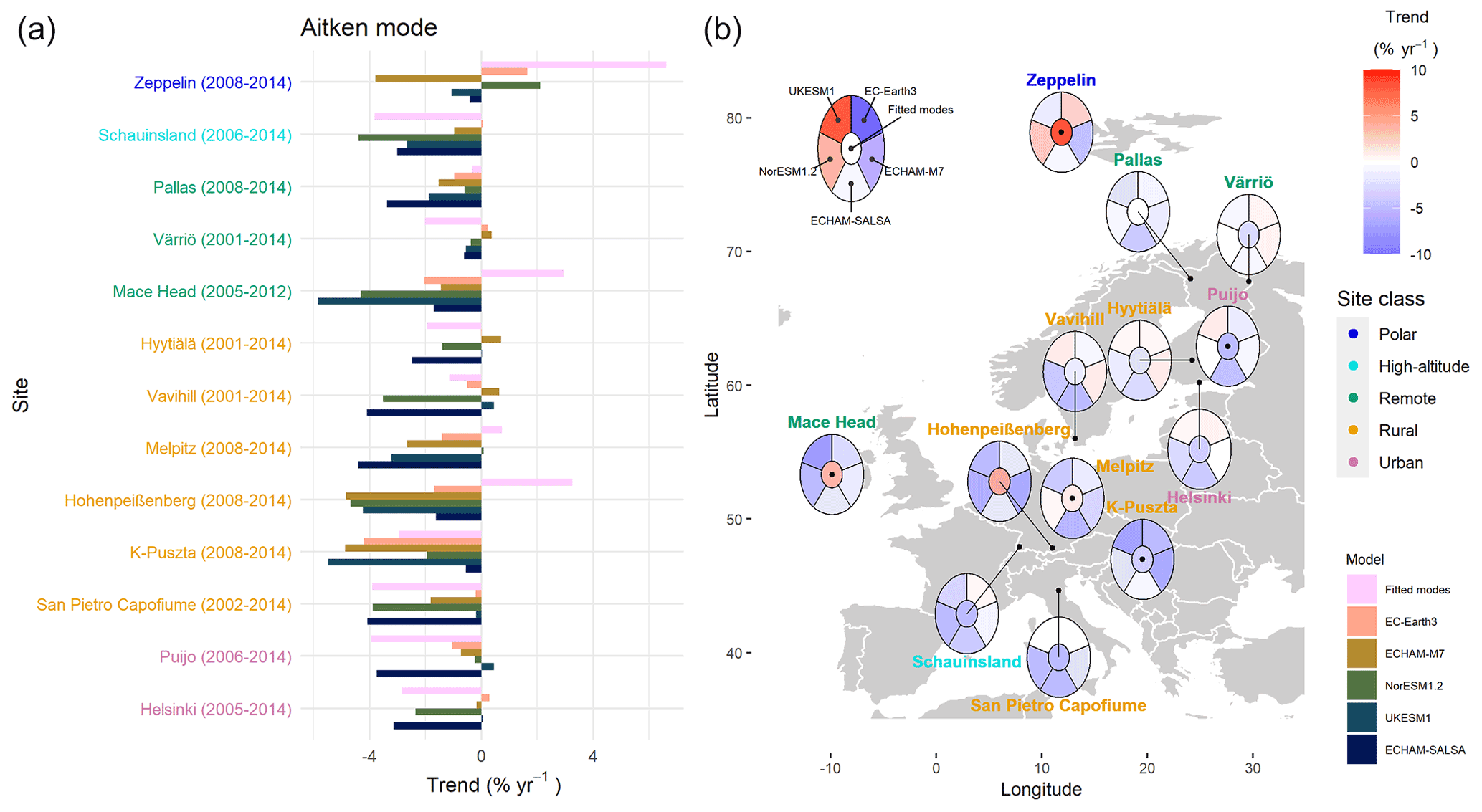
Figure 7Long-term trend estimates for measured and modelled Aitken mode number concentration. (a) Bar plot of trends at different sites. Sites (y axis) are arranged by site class and within site class most northerly to most southerly. (b) Estimated trends presented on the map. The colour of the central part follows the trend of the fitted modes. Trends have been calculated using the Sen–Theil estimator and complemented with bootstrap confidence intervals (see Sect. 2.3.2).
Most model trends for Aitken mode at sites in northern Europe were not statistically significant, while for the rest of the European sites, most trends were significant (Figs. 7 and S13). Interestingly, the sectional model ECHAM-SALSA showed a significantly decreasing trend at most of the northern sites. This might be due to the different size limits used in the modal and sectional models. At most sites where both measurement and model trends were significant, the models agreed quite well with the measurements in both strength and direction of the trend. However, Hohenpeißenberg was an exception where measurements showed a strong increasing trend, while the modelled trends were negative. The reasons for these differences are not clear.
Figure 8 shows the yearly trends in accumulation mode N; exact numbers for trends are shown in Fig. S13. Again, for most measurement sites, the different representations of the measurement data showed statistically significant trends of equal direction and similar strength. Exceptions were Melpitz and Hohenpeißenberg, which showed fairly weak, insignificant trends altogether; Zeppelin, which showed strong, opposite but, due to high variance, not statistically significant trends; and Puijo, which showed strong positive (but only partly significant) trends for all representations.
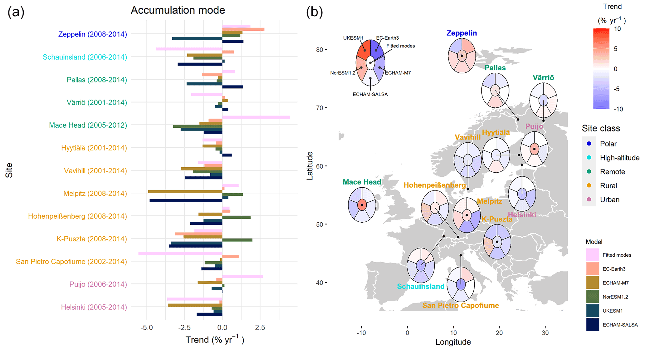
Figure 8Long-term trend estimates for measured and modelled accumulation mode number concentration. (a) Bar plot of trends at different sites. Sites (y axis) are arranged by site class and within each site class from north to south. (b) Estimated trends presented on the map. The colour of the central part follows the trend of the fitted modes. Trends have been calculated using the Sen–Theil estimator and complemented with bootstrap confidence intervals (see Sect. 2.3.2).
Concerning the model data, we did not find trends at any of the measurement sites that were statistically significant in the models. A general but weak tendency was that occurrence of statistical significance increased with decreasing latitude of the site. However, this tendency was not systematic in terms of which model produced significance at which site. Additionally, accumulation mode N depends on wildfire, sea salt, and mineral dust emissions (and atmospheric processes such as cloud processing) and hence on the means of how these emissions are calculated and inserted into the model atmosphere. Considering these factors in combination with the relatively short period analysed here, a strong model internal and inter-model variability is to be expected.
There were only two sites, Helsinki and Vavihill, where all models and measurement representations agreed on the direction of the trend (negative in both cases) in accumulation mode N (Figs. 8 and S13). Some sites stood out because the different models found strong trends in opposite directions there. Hohenpeißenberg and K-Puszta stood out, as here the model trends were mainly negative except for NorESM1.2, which showed positive (albeit not significant) trends for both sites, as was also already discussed in connection with the nucleation mode trends.
In general, the agreement between models and observations in trends of N for all modes varied a lot within the site classes, and no specific factor explaining the variation was found (see Figs. S14–S16).
3.2.2 Comparison of seasonal trends
Figures 9 and 10 show the seasonal trends for Aitken and accumulation mode N, respectively, at all measurement sites analysed in Sect. 3.2.1. Results for nucleation mode are shown in Fig. S17. Seasonal trends of N included more uncertainty than yearly average trends due to fewer data points. Particularly the modelling results rarely showed statistically significant trends, even though the actual magnitudes of the calculated trends were often quite large. In general, the trends derived for the measurement data did not depend strongly on the representation used. The few exceptions to this were Aitken mode trends at Zeppelin, Pallas, and Melpitz and accumulation mode trends at Zeppelin and Hohenpeißenberg. Seasonal model trends varied quite a lot between models, depending on the season, mode, and measurement site. We found that the differences between the models and observations and between models were largest for the sites where the observations show a strong positive trend (Zeppelin, Mace Head, and Hohenpeißenberg). For such stations, models exhibited either negative trends or lower trends than what was observed.
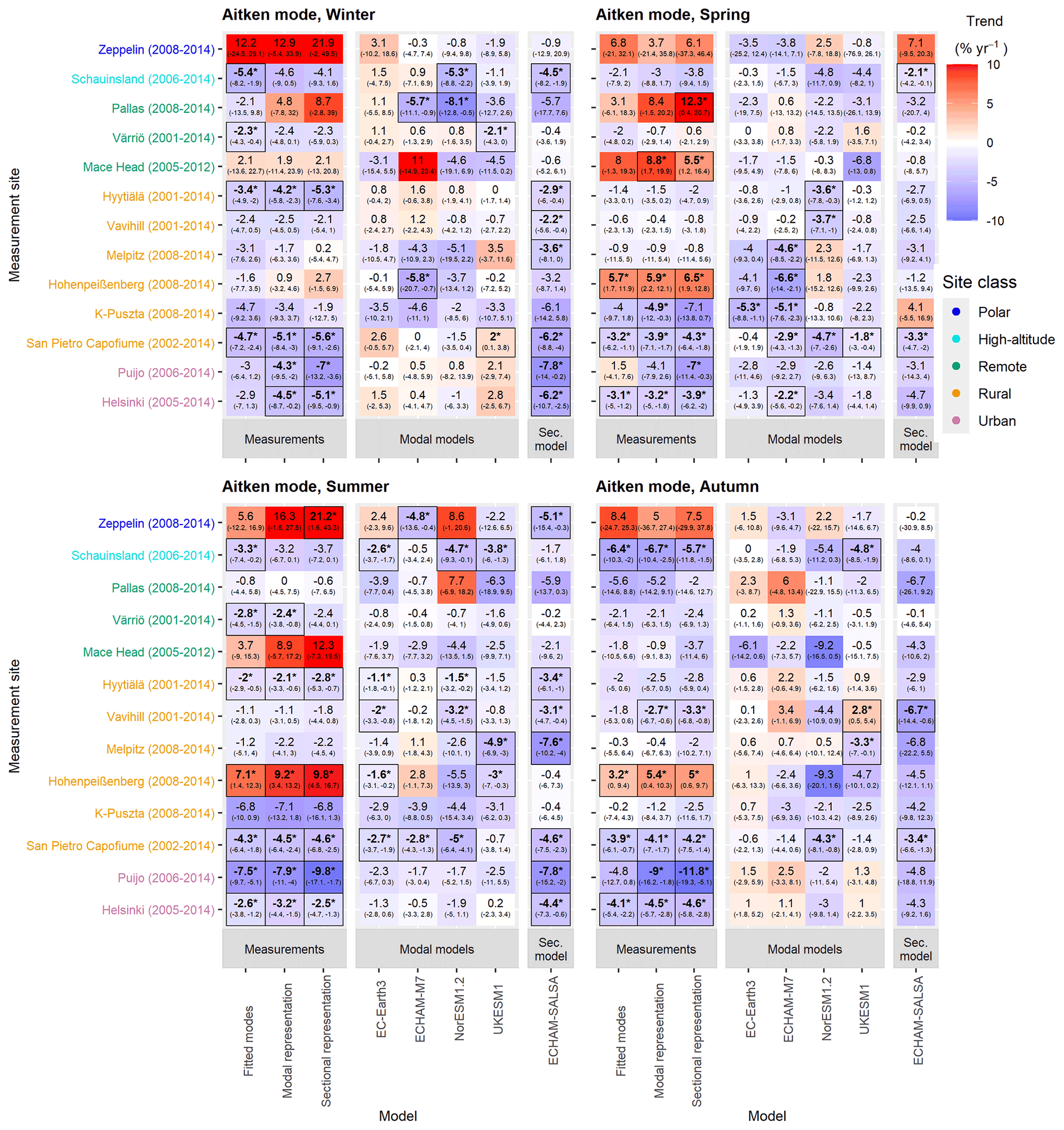
Figure 9Seasonal trend estimates for Aitken mode number concentration for four seasons: winter (January, February, December), spring (March, April, May), summer (June, July, August), and autumn (September, October, November). Sites are ordered by site class and within site class most northerly to most southerly. Bold numbers, asterisks, and line borders around the estimate indicate that the trend is statistically significant (95 % confidence level). Trends have been calculated using the Sen–Theil estimator and complemented with bootstrap confidence intervals (see Sect. 2.3.2).
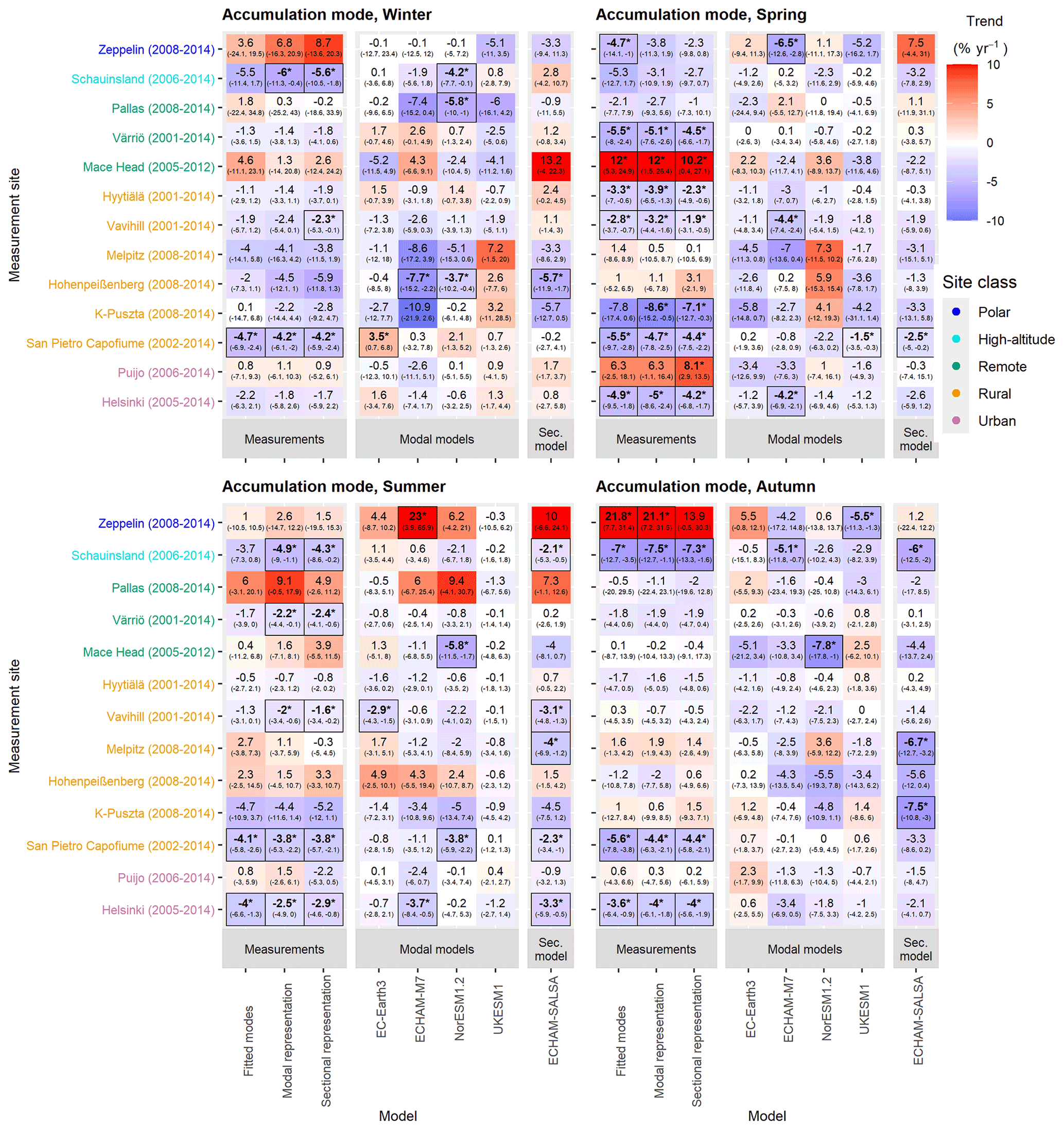
Figure 10Seasonal trend estimates for accumulation mode number concentration for four seasons: winter (January, February, December), spring (March, April, May), summer (June, July, August), and autumn (September, October, November). Sites are ordered by site class and within site class from most northerly to most southerly. Bold numbers, asterisks, and line borders around the estimate indicate that the trend is statistically significant (95 % confidence level). Trends have been calculated using the Sen–Theil estimator and complemented with bootstrap confidence intervals (see Sect. 2.3.2).
Apart from a few exceptions, the measurements showed decreasing seasonal trends of the Aitken mode N, which were also significant for some sites (Fig. 9). The exceptions were Zeppelin, Hohenpeißenberg, and Mace Head. Additionally, the measurements at K-Puszta showed increasing trends in the autumn. In general, most of the significant model trends were negative and were found during spring and summer. Neither observed nor simulated data showed significant trends in opposite directions for any of the two seasons; i.e. the significant seasonal trends were either decreasing or increasing for the one site and one measurement or model. Insignificant trends for the same site and measurement or model were sometimes decreasing for some seasons and increasing for some other seasons. The clearest difference between trends in modelled and measured data could be seen for the sites located in Finland, especially during winter and autumn, where the measurements showed a decreasing trend, while the models mostly showed an increasing trend. Those differences observed during winter and autumn could affect the differences in yearly trends observed in Fig. 7.
There was no general agreement between different models concerning accumulation mode N trends (Fig. 10). The trends in the measurements for accumulation mode were mostly fairly similar to the Aitken mode trends. For many sites, these trends from measurements were significant only during spring. Aitken mode trends from models were mostly insignificant. As can be expected from the yearly trends, the models reproduced measurement trends rather poorly, with no model performing much better or worse than any other model.
3.2.3 Comparison of seasonality and its pattern
In this section, we describe the seasonality and its pattern for nucleation (Fig. S24), Aitken (Fig. 11), and accumulation (Fig. 12) modes. More quantitative investigation based on SeasC and NIQR described in Sect. 2.3.3 can be found in Sect. S1 in the Supplement.

Figure 11Seasonal cycle of Aitken mode number concentration in measurements and climate models for measurement sites. A subplot represents the seasonal cycle in one model or measurement. Coloured lines represent the median of the monthly means for Aitken mode number concentrations. Sites are ordered from most northerly to most southerly.
For pattern of seasonality in modelled data, two models, NorESM1.2 and EC-Earth3, had relatively consistent patterns for all sites, whereas for the other three models the seasonal cycle changed between north and south (Fig. 11 for Aitken mode and Fig. 12 for accumulation mode). NorESM1.2 and EC-Earth3 had relatively constant patterns of seasonality throughout Europe, even though the seasonal maximum variation between the sites varied. For NorESM1.2, nucleation mode had its maximum N in winter (see Fig. S24), whereas Aitken and accumulation mode had their maximum N in summer. EC-Earth3 had also consistent modes among all sites: nucleation mode had its maximum in summer; Aitken and accumulation mode had their maximum in winter or early spring.

Figure 12The seasonal cycle of accumulation mode number concentration in measurements and climate models for measurement sites. A subplot represents the seasonal cycle in one model or measurement. Coloured lines represent the median of the monthly means for accumulation mode number concentrations. Sites are ordered from most northerly to most southerly.
The other three models – ECHAM-M7, ECHAM-SALSA, and UKESM1 – showed more clear changes in the patterns of seasonality between sites, typically showing stronger seasonality at northern sites. For Aitken mode (Fig. 11), ECHAM-SALSA showed two maxima in the seasonality in Aitken mode; however the seasonality is weaker at southern sites. ECHAM-SALSA also showed two maxima for nucleation mode (Fig. S24). ECHAM-M7 showed the summer maximum for northern sites (Fig. 11), whereas for southern sites the seasonal curve was constant throughout the year or has the maximum in winter. Looking at the measurement-based representations (modal and sectional representation), the differences in seasonal patterns between the two ECHAM models were not only due to differences in Aitken mode diameter ranges. One likely contributor to the differences between M7 and SALSA was that they use different nucleation parameterizations. M7 uses the parameterization by Kazil et al. (2010), and SALSA uses the activation nucleation parameterizations by Sihto et al. (2006). In addition, it has been shown that solving simultaneously occurring nucleation and condensation within microphysical models will have implications for simulated new particle formation and growth of particles (Kokkola et al., 2009; Wan et al., 2013). Thus, the differences between M7 and SALSA are also related to differences in their numerical methods used for solving nucleation and condensation (see Kokkola et al., 2008, 2009). For the accumulation mode (Fig. 12), these three models show a summer maximum at northern sites. For southern sites, ECHAM-SALSA shows a summer maximum with a weaker seasonal effect, and UKESM1 and ECHAM-M7 show consistent seasonal curves or winter N maxima with weak seasonal effects. For nucleation mode, ECHAM-SALSA and ECHAM-M7 have two maxima in spring and autumn, whereas UKESM1 has typically only one maximum in winter or early spring (Fig. S24).
Additionally, modelled N's for different sites and the ratio between the highest- and lowest-concentration sites varied significantly between the models. Differences in Aitken mode N's between models can be due to differences in model microphysics (see Table 3), and especially in accumulation mode these differences can be due to varying deposition rates that affect the efficiency of long-range transportation of particles or the way emissions are divided into different size ranges. Differences were large, especially in Aitken mode, when we compared how N's were distributed between the sites in models and measurements. Furthermore, there were large variations in measured concentrations between the sites for all three investigated modes. The ratio for Aitken mode yearly median concentrations between the highest- and lowest-concentration sites was between 65 and 90 for different measurement-based representations (fitted modes, modal and sectional representation) and between 4 and 180 for models (see also Fig. 11). For Aitken mode, ECHAM models had the least variation in concentrations between sites, followed by EC-Earth3, UKESM1, and NorESM1.2. For accumulation mode, ratios were smaller, between 34 and 40 for measurement-based representations and between 11 and 111 for models. For accumulation mode, the ratios were between 11 and 15 for UKESM1, EC-Earth3, and ECHAM-M7; 58 for ECHAM-SALSA; and 111 for NorESM1.2. A large difference between ECHAM models might be due to differences in accumulation mode diameters and low concentration of accumulation mode particles at the Zeppelin site in ECHAM-SALSA. The concentrations in sectional model representation (particle diameter 50–700 nm) were higher than for modal representation (100–1000 nm) for both ECHAM models and measurement-based representations.
In this study, we had two aims: (1) to study the trends of particle modes, namely nucleation, Aitken, and accumulation, and their properties (N, Dp, σ) in Europe and the Arctic and (2) to provide the first extensive comparison for climate model aerosol number concentration trends and seasonality with measured ones. In addition to providing a data set for model evaluation, the observational data compiled in this study could also facilitate studies on how the aerosol size distributions have evolved during previous years and how they have changed, e.g. the cloud activation capability of aerosol.
The results for measured data sets were in line with previous studies, showing that the number concentrations of particles were usually higher at urban sites and southern and central Europe than at rural sites in northern Europe. Additionally, our results from measurements showed a decreasing trend for most of the mode number concentrations and sites, which supports earlier findings. Our investigation for mode fittings revealed that mode diameter and number concentrations are dependent: increasing number concentration was sometimes related to a decrease in mode mean diameter. This dependency was stronger for particles of smaller diameters.
We also found that the trends in measured number concentrations differ between seasons and that the sign and the magnitude of the trend were not constant during the time period. The dynamic linear model (DLM) model was applied to characterize the changes in trends. DLM results supported our finding of dependence of diameter and number concentration in mode-fitting data. In addition, we found that the changes in parameters are site-specific; i.e. time periods of decrease and at the same time increase among other sites of the same area were found. On the other hand, sites are considered to be point measurements, which means that if decreases in the particle properties would have been observed at the same time in a certain area, it should have resulted from uniform changes in the particle properties at a regional level.
We compared measured and modelled trends for aerosol number concentrations. The measured trends were made comparable with global model results by calculating corresponding sectional and modal representations also from the measured data. It was seen that the factors affecting the fitted modes, namely larger diameters in fitted modes and correlations between the mean diameter and number concentration, did not have a large role in the estimated trends from the measured data. Trend estimates for mode-fitting data and corresponding sectional and modal representations were close to each other. For some sites, long-term measurements of small (<10 nm) particles were not available; thus, conclusions about the nucleation mode trends for those sites were uncertain.
We found that models were mostly able to reproduce long-term decreasing trends in Aitken and accumulation modes. Modelled trends of yearly data were usually smaller in absolute value but had the same direction as measured trends for most of the sites. We found that the differences between the models and observations were largest for the sites where the observations show a strong positive trend (Zeppelin, Mace Head, and Hohenpeißenberg). We assume that those sites may represent more local conditions than the area captured by the climate model grid box. For seasonal trends in general, the differences were larger. However, the number of data points in seasonal trend estimation is relatively small. In general, the agreement between the models and observations varied a lot within the site classes, and no specific factor explaining the variation was found.
For seasonality representation, we found models with differences in their representation despite the anthropogenic mass emissions used in models being the same. There were differences in the seasonal pattern, its magnitude, and when the maxima of number concentrations are achieved. Furthermore, for some models, the seasonal pattern was relatively uniform for all the sites, whereas for other models, the seasonal pattern varied between sites: for ECHAM-M7, ECHAM-SALSA, and UKESM1, the seasonal pattern varied between sites, while for EC-Earth3 and NorESM1.2, the pattern was consistent for all sites. Also, the modelled number concentrations for different models had large differences. In general, we found that the seasonality analysed from models and its differences between the sites did not depend solely on emissions used in the models or, for example, on aerosol size distribution representation (sectional or modal), but it is likely that the seasonality behaviour is driven by representation of different physical processes and their interplay. Also, the differences in modelled N of Aitken and accumulation particles suggest that the modelled microphysics, e.g. particle deposition rates and long-range transportation, could explain some of the differences in the Aitken and accumulation mode N, and this effect should be studied separately. Our results indicate that the availability and nature of the observations we have limit our ability to understand whether the models accurately represent trends in particle concentrations and how this, in turn, affects ACI. In addition to consistent long-term data, good characterization of the measurement sites and the surrounding areas that they present is important for a thorough comparison between models and observations. We suggest that a more detailed characterization of processes causing model differences should be conducted in the future. It would be important to study the effect of other individual aerosol processes of the models on the modelled aerosol number concentrations to extract the most important reasons for the differences.
Most of the particle number size distribution measurement data sets are already available from ACTRIS (https://actris.nilu.no/, last access: 31 July 2019; NILU, 2019) and SmartSmear (https://smear.avaa.csc.fi/, last access: 9 October 2019; Ministry of Education and Culture of Finland and CSC, 2019) databases. Data from Nieminen et al. (2018; https://doi.org/10.5194/acp-18-14737-2018), missing measurement sites (Järvselja, San Pietro Capofiume, Villum), and model data as well as the codes are available upon request from the authors.
The supplement related to this article is available online at: https://doi.org/10.5194/acp-22-12873-2022-supplement.
HK, TYJ, TK, TN, AV, and SM planned the analysis; HK, TeM, TK, TB, KC, SD, MF, TH, NK, RK, MK, AL, AM, NM, JPM, SMN, TvN, FMO, CO, DO, JBP, TP, ØS, MS, CS, HS, ES, TT, and AW participated in data collection; VL, SH, and TuM wrote the code for data analysis; VL, HK, TYJ, TeM, TK, TN, AV, and SM performed data analysis, analysed the results, and contributed to the writing of the original draft, with comments from all co-authors.
At least one of the (co-)authors is a member of the editorial board of Atmospheric Chemistry and Physics. The peer-review process was guided by an independent editor, and the authors also have no other competing interests to declare.
Publisher’s note: Copernicus Publications remains neutral with regard to jurisdictional claims in published maps and institutional affiliations.
The Villum Foundation is gratefully acknowledged for financing the establishment of Villum Research. Thanks to the Royal Danish Air Force and the Arctic Command for providing logistic support to the project. Christel Christoffersen, Bjarne Jensen, and Keld Mortensen are gratefully acknowledged for their technical support.
This research has been supported by the European Union's Horizon 2020 research and innovation programme under grant agreement nos. 821205 (FORCeS) and 641816 (CRESCENDO), Academy of Finland Flagship funding (grant nos. 337550, 337552, and 337549), and the Academy of Finland competitive funding to strengthen university research profiles (PROFI) for the University of Eastern Finland (grant no. 325022). The research leading to these results has received funding from the European Union's Horizon 2020 research and innovation programme under grant agreement nos. 262254 (ACTRIS), 654109 (ACTRIS-2), 739530 (ACTRIS-PPP), 871115 (ACTRIS-IMP), and 689443 (ERA-PLANET). Tero Mielonen's and Harri Kokkola's work was supported by the Academy of Finland (grant nos. 308292 and 317390). Steffen M. Noe was supported by the Estonian Ministry of Sciences projects (grant nos. P180021, P180274, and P200196) and by the Estonian Research Infrastructures Roadmap Project “Estonian Environmental Observatory” (3.2.0304.11-0395). Fiona M. O'Connor was supported by the BEIS and DEFRA Met Office Hadley Centre Climate Programme (GA01101). Catherine E. Scott received funding from the UK's Natural Environment Research Council under NE/S015396/1. Erik Swietlicki was supported by the Swedish Research Council (Vetenskapsrådet) for ACTRIS Sweden under contract 2021-00177. This research has been partly financially supported by the Danish Environmental Protection Agency and the Danish Energy Agency with means from MIKA/DANCEA funds for environmental support to the Arctic region (project nos. Danish EPA: MST-113-00-140; Ministry of Climate, Energy, and Utilities: 2018-3767) and ERA-PLANET (the European network for observing our changing Planet) projects; iGOSP and iCUPE; and finally the Graduate School of Science and Technology, Aarhus University.
This paper was edited by Lynn M. Russell and reviewed by two anonymous referees.
Anderson, T. R., Spall, S. A., Yool, A., Cipollini, P., Challenor, P. G., and Fasham, M. J. R.: Global fields of sea surface dimethylsulfide predicted from chlorophyll, nutrients and light, J. Marine Syst., 30, 1–20, https://doi.org/10.1016/S0924-7963(01)00028-8, 2001.
Andres, R. J. and Kasgnoc, A. D.: A time-averaged inventory of subaerial volcanic sulfur emissions, J. Geophys. Res.-Atmos., 103, 25251–25261, https://doi.org/10.1029/98JD02091, 1998.
Archibald, A. T., O'Connor, F. M., Abraham, N. L., Archer-Nicholls, S., Chipperfield, M. P., Dalvi, M., Folberth, G. A., Dennison, F., Dhomse, S. S., Griffiths, P. T., Hardacre, C., Hewitt, A. J., Hill, R. S., Johnson, C. E., Keeble, J., Köhler, M. O., Morgenstern, O., Mulcahy, J. P., Ordóñez, C., Pope, R. J., Rumbold, S. T., Russo, M. R., Savage, N. H., Sellar, A., Stringer, M., Turnock, S. T., Wild, O., and Zeng, G.: Description and evaluation of the UKCA stratosphere–troposphere chemistry scheme (StratTrop vn 1.0) implemented in UKESM1, Geosci. Model Dev., 13, 1223–1266, https://doi.org/10.5194/gmd-13-1223-2020, 2020.
Arneth, A., Harrison, S. P., Zaehle, S., Tsigaridis, K., Menon, S., Bartlein, P. J., Feichter, J., Korhola, A., Kulmala, M., O'Donnell, D., Schurgers, G., Sorvari, S., and Vesala, T.: Terrestrial biogeochemical feedbacks in the climate system, Nat. Geosci., 3, 525–532, https://doi.org/10.1038/ngeo905, 2010.
Asmi, A., Wiedensohler, A., Laj, P., Fjaeraa, A.-M., Sellegri, K., Birmili, W., Weingartner, E., Baltensperger, U., Zdimal, V., Zikova, N., Putaud, J.-P., Marinoni, A., Tunved, P., Hansson, H.-C., Fiebig, M., Kivekäs, N., Lihavainen, H., Asmi, E., Ulevicius, V., Aalto, P. P., Swietlicki, E., Kristensson, A., Mihalopoulos, N., Kalivitis, N., Kalapov, I., Kiss, G., de Leeuw, G., Henzing, B., Harrison, R. M., Beddows, D., O'Dowd, C., Jennings, S. G., Flentje, H., Weinhold, K., Meinhardt, F., Ries, L., and Kulmala, M.: Number size distributions and seasonality of submicron particles in Europe 2008–2009, Atmos. Chem. Phys., 11, 5505–5538, https://doi.org/10.5194/acp-11-5505-2011, 2011.
Asmi, A., Collaud Coen, M., Ogren, J. A., Andrews, E., Sheridan, P., Jefferson, A., Weingartner, E., Baltensperger, U., Bukowiecki, N., Lihavainen, H., Kivekäs, N., Asmi, E., Aalto, P. P., Kulmala, M., Wiedensohler, A., Birmili, W., Hamed, A., O'Dowd, C., G Jennings, S., Weller, R., Flentje, H., Fjaeraa, A. M., Fiebig, M., Myhre, C. L., Hallar, A. G., Swietlicki, E., Kristensson, A., and Laj, P.: Aerosol decadal trends – Part 2: In-situ aerosol particle number concentrations at GAW and ACTRIS stations, Atmos. Chem. Phys., 13, 895–916, https://doi.org/10.5194/acp-13-895-2013, 2013.
Bentsen, M., Bethke, I., Debernard, J. B., Iversen, T., Kirkevåg, A., Seland, Ø., Drange, H., Roelandt, C., Seierstad, I. A., Hoose, C., and Kristjánsson, J. E.: The Norwegian Earth System Model, NorESM1-M – Part 1: Description and basic evaluation of the physical climate, Geosci. Model Dev., 6, 687–720, https://doi.org/10.5194/gmd-6-687-2013, 2013.
Bergman, T., Makkonen, R., Schrödner, R., Swietlicki, E., Phillips, V. T. J., Le Sager, P., and van Noije, T.: Description and evaluation of a secondary organic aerosol and new particle formation scheme within TM5-MP v1.2, Geosci. Model Dev., 15, 683–713, https://doi.org/10.5194/gmd-15-683-2022, 2022.
Berrisford, P., Kållberg, P., Kobayashi, S., Dee, D., Uppala, S., Simmons, A. J., Poli, P., and Sato, H.: Atmospheric conservation properties in ERA-Interim, Q. J. Roy. Meteor. Soc., 137, 1381–1399, https://doi.org/10.1002/qj.864, 2011.
Birmili, W., Berresheim, H., Plass-Dülmer, C., Elste, T., Gilge, S., Wiedensohler, A., and Uhrner, U.: The Hohenpeissenberg aerosol formation experiment (HAFEX): a long-term study including size-resolved aerosol, H2SO4, OH, and monoterpenes measurements, Atmos. Chem. Phys., 3, 361–376, https://doi.org/10.5194/acp-3-361-2003, 2003.
Birmili, W., Weinhold, K., Rasch, F., Sonntag, A., Sun, J., Merkel, M., Wiedensohler, A., Bastian, S., Schladitz, A., Löschau, G., Cyrys, J., Pitz, M., Gu, J., Kusch, T., Flentje, H., Quass, U., Kaminski, H., Kuhlbusch, T. A. J., Meinhardt, F., Schwerin, A., Bath, O., Ries, L., Gerwig, H., Wirtz, K., and Fiebig, M.: Long-term observations of tropospheric particle number size distributions and equivalent black carbon mass concentrations in the German Ultrafine Aerosol Network (GUAN), Earth Syst. Sci. Data, 8, 355–382, https://doi.org/10.5194/essd-8-355-2016, 2016.
Bouwman, A. F., Lee, D. S., Asman, W. A. H., Dentener, F. J., Van Der Hoek, K. W., and Olivier, J. G. J.: A global high-resolution emission inventory for ammonia, Global Biogeochem. Cy., 11, 561–587, https://doi.org/10.1029/97GB02266, 1997.
Breider, T. J., Mickley, L. J., Jacob, D. J., Ge, C., Wang, J., Sulprizio, M. P., Croft, B., Ridley, D. A., McConnell, J. R., Sharma, S., Husain, L., Dutkiewicz, V. A., Eleftheriadis, K., Skov, H., and Hopke, P. K.: Multidecadal trends in aerosol radiative forcing over the Arctic: Contribution of changes in anthropogenic aerosol to Arctic warming since 1980, J. Geophys. Res., 122, 3573–3594, https://doi.org/10.1002/2016JD025321, 2017.
Carslaw, D. C. and Ropkins, K.: openair — An R package for air quality data analysis, Environ. Modell. Softw., 27–28, 52–61, https://doi.org/10.1016/j.envsoft.2011.09.008, 2012.
Cheng, T., Peng, Y., Feichter, J., and Tegen, I.: An improvement on the dust emission scheme in the global aerosol-climate model ECHAM5-HAM, Atmos. Chem. Phys., 8, 1105–1117, https://doi.org/10.5194/acp-8-1105-2008, 2008.
Collaud Coen, M., Andrews, E., Asmi, A., Baltensperger, U., Bukowiecki, N., Day, D., Fiebig, M., Fjaeraa, A. M., Flentje, H., Hyvärinen, A., Jefferson, A., Jennings, S. G., Kouvarakis, G., Lihavainen, H., Lund Myhre, C., Malm, W. C., Mihapopoulos, N., Molenar, J. V., O'Dowd, C., Ogren, J. A., Schichtel, B. A., Sheridan, P., Virkkula, A., Weingartner, E., Weller, R., and Laj, P.: Aerosol decadal trends – Part 1: In-situ optical measurements at GAW and IMPROVE stations, Atmos. Chem. Phys., 13, 869–894, https://doi.org/10.5194/acp-13-869-2013, 2013.
Collaud Coen, M., Andrews, E., Alastuey, A., Arsov, T. P., Backman, J., Brem, B. T., Bukowiecki, N., Couret, C., Eleftheriadis, K., Flentje, H., Fiebig, M., Gysel-Beer, M., Hand, J. L., Hoffer, A., Hooda, R., Hueglin, C., Joubert, W., Keywood, M., Kim, J. E., Kim, S.-W., Labuschagne, C., Lin, N.-H., Lin, Y., Lund Myhre, C., Luoma, K., Lyamani, H., Marinoni, A., Mayol-Bracero, O. L., Mihalopoulos, N., Pandolfi, M., Prats, N., Prenni, A. J., Putaud, J.-P., Ries, L., Reisen, F., Sellegri, K., Sharma, S., Sheridan, P., Sherman, J. P., Sun, J., Titos, G., Torres, E., Tuch, T., Weller, R., Wiedensohler, A., Zieger, P., and Laj, P.: Multidecadal trend analysis of in situ aerosol radiative properties around the world, Atmos. Chem. Phys., 20, 8867–8908, https://doi.org/10.5194/acp-20-8867-2020, 2020.
Dentener, F., Kinne, S., Bond, T., Boucher, O., Cofala, J., Generoso, S., Ginoux, P., Gong, S., Hoelzemann, J. J., Ito, A., Marelli, L., Penner, J. E., Putaud, J.-P., Textor, C., Schulz, M., van der Werf, G. R., and Wilson, J.: Emissions of primary aerosol and precursor gases in the years 2000 and 1750 prescribed data-sets for AeroCom, Atmos. Chem. Phys., 6, 4321–4344, https://doi.org/10.5194/acp-6-4321-2006, 2006.
Durbin, J. and Koopman, S. J.: Time Series Analysis by State Space Methods, Oxford University Press, Oxford, ISBN 978-0-19-964117-8, 2012.
Dusek, U., Frank, G. P., Hildebrandt, L., Curtius, J., Schneider, J., Walter, S., Chand, D., Drewnick, F., Hings, S., Jung, D., Borrmann, S., and Andreae, M. O.: Size matters more than chemistry for cloud-nucleating ability of aerosol particles, Science, 312, 1375–1378, https://doi.org/10.1126/science.1125261, 2006.
Forster, P., Storelvmo, T., Armour, K., Collins, W., Dufresne, J. L., Frame, D., Lunt, D. J., Mauritsen, T., Palmer, M. D., Watanabe, M., Wild, M., and Zhang, H.: The Earth’s Energy Budget, Climate Feedbacks, and Climate Sensitivity, in: Climate Change 2021: The Physical Science Basis. Contribution of Working Group I to the Sixth Assessment Report of the Intergovernmental Panel on Climate Change, edited by: Masson-Delmotte, V., Zhai, P., Pirani, A., Connors, S. L., Péan, C., Berger, S., Caud, N., Chen, Y., Goldfarb, L., Gomis, M. I., Huang, H., Leitzell, K., Lonnoy, E., Matthews, J. B. R., Maycock, T. K., Waterfield, T., Yelekçi, O., Yu, R., and Zhou, B., Cambridge University Press, Cambridge, United Kingdom and New York, NY, USA, 923–1054, 2021.
Gantt, B., Meskhidze, N., Facchini, M. C., Rinaldi, M., Ceburnis, D., and O'Dowd, C. D.: Wind speed dependent size-resolved parameterization for the organic mass fraction of sea spray aerosol, Atmos. Chem. Phys., 11, 8777–8790, https://doi.org/10.5194/acp-11-8777-2011, 2011.
Gantt, B., Johnson, M. S., Meskhidze, N., Sciare, J., Ovadnevaite, J., Ceburnis, D., and O'Dowd, C. D.: Model evaluation of marine primary organic aerosol emission schemes, Atmos. Chem. Phys., 12, 8553–8566, https://doi.org/10.5194/acp-12-8553-2012, 2012.
Gliß, J., Mortier, A., Schulz, M., Andrews, E., Balkanski, Y., Bauer, S. E., Benedictow, A. M. K., Bian, H., Checa-Garcia, R., Chin, M., Ginoux, P., Griesfeller, J. J., Heckel, A., Kipling, Z., Kirkevåg, A., Kokkola, H., Laj, P., Le Sager, P., Lund, M. T., Lund Myhre, C., Matsui, H., Myhre, G., Neubauer, D., van Noije, T., North, P., Olivié, D. J. L., Rémy, S., Sogacheva, L., Takemura, T., Tsigaridis, K., and Tsyro, S. G.: AeroCom phase III multi-model evaluation of the aerosol life cycle and optical properties using ground- and space-based remote sensing as well as surface in situ observations, Atmos. Chem. Phys., 21, 87–128, https://doi.org/10.5194/acp-21-87-2021, 2021.
Gong, S. L.: A parameterization of sea-salt aerosol source function for sub- and super-micron particles, Global Biogeochem. Cy., 17, 1097, https://doi.org/10.1029/2003gb002079, 2003.
Guelle, W., Schulz, M., Balkanski, Y., and Dentener, F.: Influence of the source formulation on modeling the atmospheric global distribution of sea salt aerosol, J. Geophys. Res.-Atmos., 106, 27509–27524, https://doi.org/10.1029/2001JD900249, 2001.
Guenther, A., Hewitt, C. N., Erickson, D., Fall, R., Geron, C., Graedel, T., Harley, P., Klinger, L., Lerdau, M., Mckay, W. A., Pierce, T., Scholes, B., Steinbrecher, R., Tallamraju, R., Taylor, J., and Zimmerman, P.: A global model of natural volatile organic compound emissions, J. Geophys. Res., 100, 8873–8892, https://doi.org/10.1029/94JD02950, 1995.
Hamed, A., Joutsensaari, J., Mikkonen, S., Sogacheva, L., Dal Maso, M., Kulmala, M., Cavalli, F., Fuzzi, S., Facchini, M. C., Decesari, S., Mircea, M., Lehtinen, K. E. J., and Laaksonen, A.: Nucleation and growth of new particles in Po Valley, Italy, Atmos. Chem. Phys., 7, 355–376, https://doi.org/10.5194/acp-7-355-2007, 2007.
Hamed, A., Birmili, W., Joutsensaari, J., Mikkonen, S., Asmi, A., Wehner, B., Spindler, G., Jaatinen, A., Wiedensohler, A., Korhonen, H., Lehtinen, K. E. J., and Laaksonen, A.: Changes in the production rate of secondary aerosol particles in Central Europe in view of decreasing SO2 emissions between 1996 and 2006, Atmos. Chem. Phys., 10, 1071–1091, https://doi.org/10.5194/acp-10-1071-2010, 2010.
Hari, P. and Kulmala, M.: Station for Measuring Ecosystem-Atmosphere Relations (SMEAR II), Boreal Environ. Res., 10, 315–322, 2005.
Heinold, B., Tegen, I., Schepanski, K., and Banks, J. R.: New developments in the representation of Saharan dust sources in the aerosol–climate model ECHAM6-HAM2, Geosci. Model Dev., 9, 765–777, https://doi.org/10.5194/gmd-9-765-2016, 2016.
Hellén, H., Praplan, A. P., Tykkä, T., Ylivinkka, I., Vakkari, V., Bäck, J., Petäjä, T., Kulmala, M., and Hakola, H.: Long-term measurements of volatile organic compounds highlight the importance of sesquiterpenes for the atmospheric chemistry of a boreal forest, Atmos. Chem. Phys., 18, 13839–13863, https://doi.org/10.5194/acp-18-13839-2018, 2018.
Hoesly, R. M., Smith, S. J., Feng, L., Klimont, Z., Janssens-Maenhout, G., Pitkanen, T., Seibert, J. J., Vu, L., Andres, R. J., Bolt, R. M., Bond, T. C., Dawidowski, L., Kholod, N., Kurokawa, J.-I., Li, M., Liu, L., Lu, Z., Moura, M. C. P., O'Rourke, P. R., and Zhang, Q.: Historical (1750–2014) anthropogenic emissions of reactive gases and aerosols from the Community Emissions Data System (CEDS), Geosci. Model Dev., 11, 369–408, https://doi.org/10.5194/gmd-11-369-2018, 2018.
Hussein, T., Dal Maso, M., Petäjä, T., Koponen, I. K., Paatero, P., Aalto, P. P., Hämeri, K., and Kulmala, M.: Evaluation of an automatic algorithm for fitting the particle number size distributions, Boreal Environ. Res., 10, 337–355, 2005.
Hussein, T., Martikainen, J., Junninen, H., Sogacheva, L., Wagner, R., Dal Maso, M., Riipinen, I., Aalto, P. P., and Kulmala, M.: Observation of regional new particle formation in the urban atmosphere, Tellus B, 60, 509–521, https://doi.org/10.1111/j.1600-0889.2008.00365.x, 2008.
Kazil, J., Stier, P., Zhang, K., Quaas, J., Kinne, S., O'Donnell, D., Rast, S., Esch, M., Ferrachat, S., Lohmann, U., and Feichter, J.: Aerosol nucleation and its role for clouds and Earth's radiative forcing in the aerosol-climate model ECHAM5-HAM, Atmos. Chem. Phys., 10, 10733–10752, https://doi.org/10.5194/acp-10-10733-2010, 2010.
Kirkevåg, A., Grini, A., Olivié, D., Seland, Ø., Alterskjær, K., Hummel, M., Karset, I. H. H., Lewinschal, A., Liu, X., Makkonen, R., Bethke, I., Griesfeller, J., Schulz, M., and Iversen, T.: A production-tagged aerosol module for Earth system models, OsloAero5.3 – extensions and updates for CAM5.3-Oslo, Geosci. Model Dev., 11, 3945–3982, https://doi.org/10.5194/gmd-11-3945-2018, 2018.
Kokkola, H., Korhonen, H., Lehtinen, K. E. J., Makkonen, R., Asmi, A., Järvenoja, S., Anttila, T., Partanen, A.-I., Kulmala, M., Järvinen, H., Laaksonen, A., and Kerminen, V.-M.: SALSA – a Sectional Aerosol module for Large Scale Applications, Atmos. Chem. Phys., 8, 2469–2483, https://doi.org/10.5194/acp-8-2469-2008, 2008.
Kokkola, H., Hommel, R., Kazil, J., Niemeier, U., Partanen, A.-I., Feichter, J., and Timmreck, C.: Aerosol microphysics modules in the framework of the ECHAM5 climate model – intercomparison under stratospheric conditions, Geosci. Model Dev., 2, 97–112, https://doi.org/10.5194/gmd-2-97-2009, 2009.
Kokkola, H., Kühn, T., Laakso, A., Bergman, T., Lehtinen, K. E. J., Mielonen, T., Arola, A., Stadtler, S., Korhonen, H., Ferrachat, S., Lohmann, U., Neubauer, D., Tegen, I., Siegenthaler-Le Drian, C., Schultz, M. G., Bey, I., Stier, P., Daskalakis, N., Heald, C. L., and Romakkaniemi, S.: SALSA2.0: The sectional aerosol module of the aerosol–chemistry–climate model ECHAM6.3.0-HAM2.3-MOZ1.0, Geosci. Model Dev., 11, 3833–3863, https://doi.org/10.5194/gmd-11-3833-2018, 2018.
Kuhlbrodt, T., Jones, C. G., Sellar, A., Storkey, D., Blockley, E., Stringer, M., Hill, R., Graham, T., Ridley, J., Blaker, A., Calvert, D., Copsey, D., Ellis, R., Hewitt, H., Hyder, P., Ineson, S., Mulcahy, J., Siahaan, A., and Walton, J.: The Low-Resolution Version of HadGEM3 GC3.1: Development and Evaluation for Global Climate, J. Adv. Model. Earth Sy., 10, 2865–2888, https://doi.org/10.1029/2018MS001370, 2018.
Kunsch, H. R.: The Jackknife and the Bootstrap for General Stationary Observations, Ann. Stat., 17, 1217–1241, https://doi.org/10.1214/aos/1176347265, 1989.
Kyrö, E.-M., Väänänen, R., Kerminen, V.-M., Virkkula, A., Petäjä, T., Asmi, A., Dal Maso, M., Nieminen, T., Juhola, S., Shcherbinin, A., Riipinen, I., Lehtipalo, K., Keronen, P., Aalto, P. P., Hari, P., and Kulmala, M.: Trends in new particle formation in eastern Lapland, Finland: effect of decreasing sulfur emissions from Kola Peninsula, Atmos. Chem. Phys., 14, 4383–4396, https://doi.org/10.5194/acp-14-4383-2014, 2014.
Laine, M.: Introduction to Dynamic Linear Models for Time Series Analysis, in: Geodetic Time Series Analysis in Earth Sciences, edited by: Montillet, M. S. and Bos, J. P., Springer, Cham, 139–156, ISBN: 978-3-030-21718-1, 2020.
Laine, M., Latva-Pukkila, N., and Kyrölä, E.: Analysing time-varying trends in stratospheric ozone time series using the state space approach, Atmos. Chem. Phys., 14, 9707–9725, https://doi.org/10.5194/acp-14-9707-2014, 2014.
Lana, A., Bell, T. G., Simó, R., Vallina, S. M., Ballabrera-Poy, J., Kettle, A. J., Dachs, J., Bopp, L., Saltzman, E. S., Stefels, J., Johnson, J. E., and Liss, P. S.: An updated climatology of surface dimethlysulfide concentrations and emission fluxes in the global ocean, Global Biogeochem. Cy., 25, GB1004, https://doi.org/10.1029/2010GB003850, 2011.
Leskinen, A., Arola, A., Komppula, M., Portin, H., Tiitta, P., Miettinen, P., Romakkaniemi, S., Laaksonen, A., and Lehtinen, K. E. J.: Seasonal cycle and source analyses of aerosol optical properties in a semi-urban environment at Puijo station in Eastern Finland, Atmos. Chem. Phys., 12, 5647–5659, https://doi.org/10.5194/acp-12-5647-2012, 2012.
Liss, P. S. and Merlivat, L.: Air-Sea Gas Exchange Rates: Introduction and Synthesis, in: The Role of Air-Sea Exchange in Geochemical Cycling, Springer Netherlands, 113–127, ISBN: 978-94-009-4738-2, 1986.
Liu, X., Ma, P.-L., Wang, H., Tilmes, S., Singh, B., Easter, R. C., Ghan, S. J., and Rasch, P. J.: Description and evaluation of a new four-mode version of the Modal Aerosol Module (MAM4) within version 5.3 of the Community Atmosphere Model, Geosci. Model Dev., 9, 505–522, https://doi.org/10.5194/gmd-9-505-2016, 2016.
Lohila, A., Penttilä, T., Jortikka, S., Aalto, T., Anttila, P., Asmi, E., Aurela, M., Hatakka, J., Hellén, H., Henttonen, H., Hänninen, P., Kilkki, J., Kyllönen, K., Laurila, T., Lepistö, A., Lihavainen, H., Makkonen, U., Paatero, J., Rask, M., Sutinen, R., Tuovinen, J.-P., Vuorenmaa, J., and Viisanen, Y.: Preface to the special issue on integrated research of atmosphere, ecosystems and environment at Pallas, Boreal Environ. Res., 20, 431–454, 2015.
Makkonen, R., Seland, Ø., Kirkevåg, A., Iversen, T., and Kristjánsson, J. E.: Evaluation of aerosol number concentrations in NorESM with improved nucleation parameterization, Atmos. Chem. Phys., 14, 5127–5152, https://doi.org/10.5194/acp-14-5127-2014, 2014.
Mann, G. W., Carslaw, K. S., Spracklen, D. V., Ridley, D. A., Manktelow, P. T., Chipperfield, M. P., Pickering, S. J., and Johnson, C. E.: Description and evaluation of GLOMAP-mode: a modal global aerosol microphysics model for the UKCA composition-climate model, Geosci. Model Dev., 3, 519–551, https://doi.org/10.5194/gmd-3-519-2010, 2010.
MATLAB: 9.7.0.1296695 (R2019b) Update 4, The MathWorks Inc., Natick, Massachusetts, 2019.
Metzger, S., Dentener, F., Pandis, S., and Lelieveld, J.: Gas/aerosol partitioning: 1. A computationally efficient model, J. Geophys. Res., 107, 4312, https://doi.org/10.1029/2001JD001102, 2002.
Mielonen, T., Portin, H., Komppula, M., Leskinen, A., Tamminen, J., Ialongo, I., Hakkarainen, J., Lehtinen, K. E. J., and Arola, A.: Biomass burning aerosols observed in Eastern Finland during the Russian wildfires in summer 2010 – Part 2: Remote sensing, Atmos. Environ., 47, 279–287, https://doi.org/10.1016/j.atmosenv.2011.07.016, 2012.
Mihalopoulos, N., Stephanou, E., Kanakidou, M., Pilitsidis, S., and Bousquet, P.: Tropospheric aerosol ionic composition in the Eastern Mediterranean region, Tellus B, 49, 314–326, https://doi.org/10.3402/tellusb.v49i3.15970, 1997.
Mikkonen, S., Németh, Z., Varga, V., Weidinger, T., Leinonen, V., Yli-Juuti, T., and Salma, I.: Decennial time trends and diurnal patterns of particle number concentrations in a central European city between 2008 and 2018, Atmos. Chem. Phys., 20, 12247–12263, https://doi.org/10.5194/acp-20-12247-2020, 2020.
Ministry of Education and Culture of Finland and CSC: SmartSMEAR, Fairdata.fi, https://smear.avaa.csc.fi/, last access: 9 October 2019.
Mortier, A., Gliß, J., Schulz, M., Aas, W., Andrews, E., Bian, H., Chin, M., Ginoux, P., Hand, J., Holben, B., Zhang, H., Kipling, Z., Kirkevåg, A., Laj, P., Lurton, T., Myhre, G., Neubauer, D., Olivié, D., von Salzen, K., Skeie, R. B., Takemura, T., and Tilmes, S.: Evaluation of climate model aerosol trends with ground-based observations over the last 2 decades – an AeroCom and CMIP6 analysis, Atmos. Chem. Phys., 20, 13355–13378, https://doi.org/10.5194/acp-20-13355-2020, 2020.
Moseid, K. O., Schulz, M., Storelvmo, T., Julsrud, I. R., Olivié, D., Nabat, P., Wild, M., Cole, J. N. S., Takemura, T., Oshima, N., Bauer, S. E., and Gastineau, G.: Bias in CMIP6 models as compared to observed regional dimming and brightening, Atmos. Chem. Phys., 20, 16023–16040, https://doi.org/10.5194/acp-20-16023-2020, 2020.
Mulcahy, J. P., Johnson, C., Jones, C. G., Povey, A. C., Scott, C. E., Sellar, A., Turnock, S. T., Woodhouse, M. T., Abraham, N. L., Andrews, M. B., Bellouin, N., Browse, J., Carslaw, K. S., Dalvi, M., Folberth, G. A., Glover, M., Grosvenor, D. P., Hardacre, C., Hill, R., Johnson, B., Jones, A., Kipling, Z., Mann, G., Mollard, J., O'Connor, F. M., Palmiéri, J., Reddington, C., Rumbold, S. T., Richardson, M., Schutgens, N. A. J., Stier, P., Stringer, M., Tang, Y., Walton, J., Woodward, S., and Yool, A.: Description and evaluation of aerosol in UKESM1 and HadGEM3-GC3.1 CMIP6 historical simulations, Geosci. Model Dev., 13, 6383–6423, https://doi.org/10.5194/gmd-13-6383-2020, 2020.
Myhre, G., Myher, C. E. L., Samset, B. H., and Storelvmo, T.: Aerosols and their Relation to Global Climate and Climate Sensitivity, Nature Education Knowledge, 4, 7, https://www.nature.com/scitable/knowledge/library/aerosols-and-their-relation-to-global-climate-102215345/ (last access: 15 September 2022), 2013.
Neale, R. B., Chen, C.-C., Gettelman, A., Lauritzen, P. H., Park, S., Williamson, D. L., Conley, A. J., Garcia, R., Kinnison, D., Lamarque, J.-F., Marsh, D., Mills, M., Smith, A. K., Tilmes, S., Vitt, F., Morrison, H., Cameron-Smith, P., Collins, W. D., Iacono, M. J., Easter, R. C., Ghan, S. J., Liu, X., Rasch, P. J., and Taylor, M. A.: Description of the NCAR Community Atmosphere Model (CAM 5.0), NCAR TECHNICAL NOTE, NCAR/TN-486+STR, Natl. Cent. for Atmos. Res, Boulder, CO, 289 pp., 2012.
Nguyen, Q. T., Glasius, M., Sørensen, L. L., Jensen, B., Skov, H., Birmili, W., Wiedensohler, A., Kristensson, A., Nøjgaard, J. K., and Massling, A.: Seasonal variation of atmospheric particle number concentrations, new particle formation and atmospheric oxidation capacity at the high Arctic site Villum Research Station, Station Nord, Atmos. Chem. Phys., 16, 11319–11336, https://doi.org/10.5194/acp-16-11319-2016, 2016.
Nieminen, T., Kerminen, V.-M., Petäjä, T., Aalto, P. P., Arshinov, M., Asmi, E., Baltensperger, U., Beddows, D. C. S., Beukes, J. P., Collins, D., Ding, A., Harrison, R. M., Henzing, B., Hooda, R., Hu, M., Hõrrak, U., Kivekäs, N., Komsaare, K., Krejci, R., Kristensson, A., Laakso, L., Laaksonen, A., Leaitch, W. R., Lihavainen, H., Mihalopoulos, N., Németh, Z., Nie, W., O'Dowd, C., Salma, I., Sellegri, K., Svenningsson, B., Swietlicki, E., Tunved, P., Ulevicius, V., Vakkari, V., Vana, M., Wiedensohler, A., Wu, Z., Virtanen, A., and Kulmala, M.: Global analysis of continental boundary layer new particle formation based on long-term measurements, Atmos. Chem. Phys., 18, 14737–14756, https://doi.org/10.5194/acp-18-14737-2018, 2018.
Nightingale, P. D., Malin, G., Law, C. S., Watson, A. J., Liss, P. S., Liddicoat, M. I., Boutin, J., and Upstill-Goddard, R. C.: In situ evaluation of air-sea gas exchange parameterizations using novel conservative and volatile tracers, Global Biogeochem. Cy., 14, 373–387, https://doi.org/10.1029/1999GB900091, 2000.
NILU (Norwegian Institute for Air Research): The ACTRIS Data Centre web portal, NILU, https://actris.nilu.no/, last access: 31 July 2019.
Noe, S. M., Niinemets, Ü., Krasnova, A., Krasnov, D., Motallebi, A., Kängsepp, V., Jõgiste, K., Hõrrak, U., Komsaare, K., Mirme, S., Vana, M., Tammet, H., Bäck, J., Vesala, T., Kulmala, M., Petäjä, T., and Kangur, A.: SMEAR Estonia: Perspectives of a large-scale forest ecosystem – atmosphere research infrastructure, Forestry Studies, 63, 56–84, https://doi.org/10.1515/fsmu-2015-0009, 2015.
O'Connor, T. C., Jennings, S. G., and O'Dowd, C. D.: Highlights of fifty years of atmospheric aerosol research at Mace Head, Atmos. Res., 90, 338–355, https://doi.org/10.1016/j.atmosres.2008.08.014, 2008.
Paasonen, P., Asmi, A., Petäjä, T., Kajos, M. K., Äijälä, M., Junninen, H., Holst, T., Abbatt, J. P. D., Arneth, A., Birmili, W., Van Der Gon, H. D., Hamed, A., Hoffer, A., Laakso, L., Laaksonen, A., Richard Leaitch, W., Plass-Dülmer, C., Pryor, S. C., Räisänen, P., Swietlicki, E., Wiedensohler, A., Worsnop, D. R., Kerminen, V. M., and Kulmala, M.: Warming-induced increase in aerosol number concentration likely to moderate climate change, Nat. Geosci., 6, 438–442, https://doi.org/10.1038/ngeo1800, 2013.
Pacifico, F., Harrison, S. P., Jones, C. D., Arneth, A., Sitch, S., Weedon, G. P., Barkley, M. P., Palmer, P. I., Serça, D., Potosnak, M., Fu, T.-M., Goldstein, A., Bai, J., and Schurgers, G.: Evaluation of a photosynthesis-based biogenic isoprene emission scheme in JULES and simulation of isoprene emissions under present-day climate conditions, Atmos. Chem. Phys., 11, 4371–4389, https://doi.org/10.5194/acp-11-4371-2011, 2011.
Peñuelas, J. and Staudt, M.: BVOCs and global change, Trends Plant Sci., 15, 133–144, https://doi.org/10.1016/j.tplants.2009.12.005, 2010.
Petris, G., Petrone, S., and Campagnoli, P.: Dynamic linear models with R, Springer-Verlag, ISBN: 978-0-387-77238-7, 2009.
R Core Team: R: A Language and Environment for Statistical Computing, https://www.r-project.org/ (last access: 26 August 2022), 2021.
Riccobono, F., Schobesberger, S., Scott, C. E., Dommen, J., Ortega, I. K., Rondo, L., Almeida, J., Amorim, A., Bianchi, F., Breitenlechner, M., David, A., Downard, A., Dunne, E. M., Duplissy, J., Ehrhart, S., Flagan, R. C., Franchin, A., Hansel, A., Junninen, H., Kajos, M., Keskinen, H., Kupc, A., Kürten, A., Kvashin, A. N., Laaksonen, A., Lehtipalo, K., Makhmutov, V., Mathot, S., Nieminen, T., Onnela, A., Petäjä, T., Praplan, A. P., Santos, F. D., Schallhart, S., Seinfeld, J. H., Sipilä, M., Spracklen, D. V., Stozhkov, Y., Stratmann, F., Tomé, A., Tsagkogeorgas, G., Vaattovaara, P., Viisanen, Y., Vrtala, A., Wagner, P. E., Weingartner, E., Wex, H., Wimmer, D., Carslaw, K. S., Curtius, J., Donahue, N. M., Kirkby, J., Kulmala, M., Worsnop, D. R., and Baltensperger, U.: Oxidation products of biogenic emissions contribute to nucleation of atmospheric particles, Science, 344, 717–721, https://doi.org/10.1126/science.1243527, 2014.
Rose, C., Collaud Coen, M., Andrews, E., Lin, Y., Bossert, I., Lund Myhre, C., Tuch, T., Wiedensohler, A., Fiebig, M., Aalto, P., Alastuey, A., Alonso-Blanco, E., Andrade, M., Artíñano, B., Arsov, T., Baltensperger, U., Bastian, S., Bath, O., Beukes, J. P., Brem, B. T., Bukowiecki, N., Casquero-Vera, J. A., Conil, S., Eleftheriadis, K., Favez, O., Flentje, H., Gini, M. I., Gómez-Moreno, F. J., Gysel-Beer, M., Hallar, A. G., Kalapov, I., Kalivitis, N., Kasper-Giebl, A., Keywood, M., Kim, J. E., Kim, S.-W., Kristensson, A., Kulmala, M., Lihavainen, H., Lin, N.-H., Lyamani, H., Marinoni, A., Martins Dos Santos, S., Mayol-Bracero, O. L., Meinhardt, F., Merkel, M., Metzger, J.-M., Mihalopoulos, N., Ondracek, J., Pandolfi, M., Pérez, N., Petäjä, T., Petit, J.-E., Picard, D., Pichon, J.-M., Pont, V., Putaud, J.-P., Reisen, F., Sellegri, K., Sharma, S., Schauer, G., Sheridan, P., Sherman, J. P., Schwerin, A., Sohmer, R., Sorribas, M., Sun, J., Tulet, P., Vakkari, V., van Zyl, P. G., Velarde, F., Villani, P., Vratolis, S., Wagner, Z., Wang, S.-H., Weinhold, K., Weller, R., Yela, M., Zdimal, V., and Laj, P.: Seasonality of the particle number concentration and size distribution: a global analysis retrieved from the network of Global Atmosphere Watch (GAW) near-surface observatories, Atmos. Chem. Phys., 21, 17185–17223, https://doi.org/10.5194/acp-21-17185-2021, 2021.
Salma, I., Németh, Z., Kerminen, V.-M., Aalto, P., Nieminen, T., Weidinger, T., Molnár, Á., Imre, K., and Kulmala, M.: Regional effect on urban atmospheric nucleation, Atmos. Chem. Phys., 16, 8715–8728, https://doi.org/10.5194/acp-16-8715-2016, 2016.
Salter, M. E., Zieger, P., Acosta Navarro, J. C., Grythe, H., Kirkevåg, A., Rosati, B., Riipinen, I., and Nilsson, E. D.: An empirically derived inorganic sea spray source function incorporating sea surface temperature, Atmos. Chem. Phys., 15, 11047–11066, https://doi.org/10.5194/acp-15-11047-2015, 2015.
Schmale, J., Henning, S., Decesari, S., Henzing, B., Keskinen, H., Sellegri, K., Ovadnevaite, J., Pöhlker, M. L., Brito, J., Bougiatioti, A., Kristensson, A., Kalivitis, N., Stavroulas, I., Carbone, S., Jefferson, A., Park, M., Schlag, P., Iwamoto, Y., Aalto, P., Äijälä, M., Bukowiecki, N., Ehn, M., Frank, G., Fröhlich, R., Frumau, A., Herrmann, E., Herrmann, H., Holzinger, R., Kos, G., Kulmala, M., Mihalopoulos, N., Nenes, A., O'Dowd, C., Petäjä, T., Picard, D., Pöhlker, C., Pöschl, U., Poulain, L., Prévôt, A. S. H., Swietlicki, E., Andreae, M. O., Artaxo, P., Wiedensohler, A., Ogren, J., Matsuki, A., Yum, S. S., Stratmann, F., Baltensperger, U., and Gysel, M.: Long-term cloud condensation nuclei number concentration, particle number size distribution and chemical composition measurements at regionally representative observatories, Atmos. Chem. Phys., 18, 2853–2881, https://doi.org/10.5194/acp-18-2853-2018, 2018.
Schmale, J., Sharma, S., Decesari, S., Pernov, J., Massling, A., Hansson, H.-C., von Salzen, K., Skov, H., Andrews, E., Quinn, P. K., Upchurch, L. M., Eleftheriadis, K., Traversi, R., Gilardoni, S., Mazzola, M., Laing, J., and Hopke, P.: Pan-Arctic seasonal cycles and long-term trends of aerosol properties from 10 observatories, Atmos. Chem. Phys., 22, 3067–3096, https://doi.org/10.5194/acp-22-3067-2022, 2022.
Schultz, M. G., Stadtler, S., Schröder, S., Taraborrelli, D., Franco, B., Krefting, J., Henrot, A., Ferrachat, S., Lohmann, U., Neubauer, D., Siegenthaler-Le Drian, C., Wahl, S., Kokkola, H., Kühn, T., Rast, S., Schmidt, H., Stier, P., Kinnison, D., Tyndall, G. S., Orlando, J. J., and Wespes, C.: The chemistry–climate model ECHAM6.3-HAM2.3-MOZ1.0, Geosci. Model Dev., 11, 1695–1723, https://doi.org/10.5194/gmd-11-1695-2018, 2018.
Schutgens, N., Tsyro, S., Gryspeerdt, E., Goto, D., Weigum, N., Schulz, M., and Stier, P.: On the spatio-temporal representativeness of observations, Atmos. Chem. Phys., 17, 9761–9780, https://doi.org/10.5194/acp-17-9761-2017, 2017.
Schutgens, N. A. J., Partridge, D. G., and Stier, P.: The importance of temporal collocation for the evaluation of aerosol models with observations, Atmos. Chem. Phys., 16, 1065–1079, https://doi.org/10.5194/acp-16-1065-2016, 2016.
Sellar, A. A., Jones, C. G., Mulcahy, J. P., Tang, Y., Yool, A., Wiltshire, A., O'Connor, F. M., Stringer, M., Hill, R., Palmieri, J., Woodward, S., de Mora, L., Kuhlbrodt, T., Rumbold, S. T., Kelley, D. I., Ellis, R., Johnson, C. E., Walton, J., Abraham, N. L., Andrews, M. B., Andrews, T., Archibald, A. T., Berthou, S., Burke, E., Blockley, E., Carslaw, K., Dalvi, M., Edwards, J., Folberth, G. A., Gedney, N., Griffiths, P. T., Harper, A. B., Hendry, M. A., Hewitt, A. J., Johnson, B., Jones, A., Jones, C. D., Keeble, J., Liddicoat, S., Morgenstern, O., Parker, R. J., Predoi, V., Robertson, E., Siahaan, A., Smith, R. S., Swaminathan, R., Woodhouse, M. T., Zeng, G., and Zerroukat, M.: UKESM1: Description and Evaluation of the U.K. Earth System Model, J. Adv. Model. Earth Sy., 11, 4513–4558, https://doi.org/10.1029/2019MS001739, 2019.
Sen, P. K.: Estimates of the Regression Coefficient Based on Kendall's Tau, J. Am. Stat. Assoc., 63, 1379–1389, https://doi.org/10.1080/01621459.1968.10480934, 1968.
Sihto, S.-L., Kulmala, M., Kerminen, V.-M., Dal Maso, M., Petäjä, T., Riipinen, I., Korhonen, H., Arnold, F., Janson, R., Boy, M., Laaksonen, A., and Lehtinen, K. E. J.: Atmospheric sulphuric acid and aerosol formation: implications from atmospheric measurements for nucleation and early growth mechanisms, Atmos. Chem. Phys., 6, 4079–4091, https://doi.org/10.5194/acp-6-4079-2006, 2006.
Sindelarova, K., Granier, C., Bouarar, I., Guenther, A., Tilmes, S., Stavrakou, T., Müller, J.-F., Kuhn, U., Stefani, P., and Knorr, W.: Global data set of biogenic VOC emissions calculated by the MEGAN model over the last 30 years, Atmos. Chem. Phys., 14, 9317–9341, https://doi.org/10.5194/acp-14-9317-2014, 2014.
Smith, S. J. and Bond, T. C.: Two hundred fifty years of aerosols and climate: the end of the age of aerosols, Atmos. Chem. Phys., 14, 537–549, https://doi.org/10.5194/acp-14-537-2014, 2014.
Spiro, P. A., Jacob, D. J., and Logan, J. A.: Global inventory of sulfur emissions with resolution, J. Geophys. Res., 97, 6023–6036, https://doi.org/10.1029/91JD03139, 1992.
Stevens, B., Giorgetta, M., Esch, M., Mauritsen, T., Crueger, T., Rast, S., Salzmann, M., Schmidt, H., Bader, J., Block, K., Brokopf, R., Fast, I., Kinne, S., Kornblueh, L., Lohmann, U., Pincus, R., Reichler, T., and Roeckner, E.: Atmospheric component of the MPI-M Earth System Model: ECHAM6, J. Adv. Model. Earth Sy., 5, 146–172, https://doi.org/10.1002/jame.20015, 2013.
Storelvmo, T., Heede, U. K., Leirvik, T., Phillips, P. C. B., Arndt, P., and Wild, M.: Lethargic Response to Aerosol Emissions in Current Climate Models, Geophys. Res. Lett., 45, 9814–9823, https://doi.org/10.1029/2018GL078298, 2018.
Sun, J., Birmili, W., Hermann, M., Tuch, T., Weinhold, K., Merkel, M., Rasch, F., Müller, T., Schladitz, A., Bastian, S., Löschau, G., Cyrys, J., Gu, J., Flentje, H., Briel, B., Asbach, C., Kaminski, H., Ries, L., Sohmer, R., Gerwig, H., Wirtz, K., Meinhardt, F., Schwerin, A., Bath, O., Ma, N., and Wiedensohler, A.: Decreasing trends of particle number and black carbon mass concentrations at 16 observational sites in Germany from 2009 to 2018, Atmos. Chem. Phys., 20, 7049–7068, https://doi.org/10.5194/acp-20-7049-2020, 2020.
Tegen, I., Harrison, S. P., Kohfeld, K., Prentice, I. C., Coe, M., and Heimann, M.: Impact of vegetation and preferential source areas on global dust aerosol: Results from a model study, J. Geophys. Res.-Atmos., 107, AAC 14-1–AAC 14-27, https://doi.org/10.1029/2001JD000963, 2002.
Tegen, I., Neubauer, D., Ferrachat, S., Siegenthaler-Le Drian, C., Bey, I., Schutgens, N., Stier, P., Watson-Parris, D., Stanelle, T., Schmidt, H., Rast, S., Kokkola, H., Schultz, M., Schroeder, S., Daskalakis, N., Barthel, S., Heinold, B., and Lohmann, U.: The global aerosol–climate model ECHAM6.3–HAM2.3 – Part 1: Aerosol evaluation, Geosci. Model Dev., 12, 1643–1677, https://doi.org/10.5194/gmd-12-1643-2019, 2019.
Theil, H.: A rank-invariant method of linear and polynomial regression analysis, reprinted in 1992 in Henri Theil’s contributions to economics and econometrics, Springer, 345–381, https://doi.org/10.1007/978-94-011-2546-8_20, 1950
Tunved, P., Ström, J., and Krejci, R.: Arctic aerosol life cycle: linking aerosol size distributions observed between 2000 and 2010 with air mass transport and precipitation at Zeppelin station, Ny-Ålesund, Svalbard, Atmos. Chem. Phys., 13, 3643–3660, https://doi.org/10.5194/acp-13-3643-2013, 2013.
van Marle, M. J. E., Kloster, S., Magi, B. I., Marlon, J. R., Daniau, A.-L., Field, R. D., Arneth, A., Forrest, M., Hantson, S., Kehrwald, N. M., Knorr, W., Lasslop, G., Li, F., Mangeon, S., Yue, C., Kaiser, J. W., and van der Werf, G. R.: Historic global biomass burning emissions for CMIP6 (BB4CMIP) based on merging satellite observations with proxies and fire models (1750–2015), Geosci. Model Dev., 10, 3329–3357, https://doi.org/10.5194/gmd-10-3329-2017, 2017.
van Noije, T., Bergman, T., Le Sager, P., O'Donnell, D., Makkonen, R., Gonçalves-Ageitos, M., Döscher, R., Fladrich, U., von Hardenberg, J., Keskinen, J.-P., Korhonen, H., Laakso, A., Myriokefalitakis, S., Ollinaho, P., Pérez García-Pando, C., Reerink, T., Schrödner, R., Wyser, K., and Yang, S.: EC-Earth3-AerChem: a global climate model with interactive aerosols and atmospheric chemistry participating in CMIP6 , Geosci. Model Dev., 14, 5637–5668, https://doi.org/10.5194/gmd-14-5637-2021, 2021.
Vehkamäki, H.: An improved parameterization for sulfuric acid–water nucleation rates for tropospheric and stratospheric conditions, J. Geophys. Res., 107, 4622, https://doi.org/10.1029/2002JD002184, 2002.
Vignati, E., Wilson, J., and Stier, P.: M7: An efficient size-resolved aerosol microphysics module for large-scale aerosol transport models, J. Geophys. Res., 109, D22202, https://doi.org/10.1029/2003JD004485, 2004.
Wan, H., Rasch, P. J., Zhang, K., Kazil, J., and Leung, L. R.: Numerical issues associated with compensating and competing processes in climate models: an example from ECHAM-HAM, Geosci. Model Dev., 6, 861–874, https://doi.org/10.5194/gmd-6-861-2013, 2013.
Wanninkhof, R.: Relationship between wind speed and gas exchange over the ocean revisited, Limnol. Oceanogr.-Meth., 12, 351–362, https://doi.org/10.4319/lom.2014.12.351, 2014.
Williams, J., de Reus, M., Krejci, R., Fischer, H., and Ström, J.: Application of the variability-size relationship to atmospheric aerosol studies: estimating aerosol lifetimes and ages, Atmos. Chem. Phys., 2, 133–145, https://doi.org/10.5194/acp-2-133-2002, 2002.
Williams, K. D., Copsey, D., Blockley, E. W., Bodas-Salcedo, A., Calvert, D., Comer, R., Davis, P., Graham, T., Hewitt, H. T., Hill, R., Hyder, P., Ineson, S., Johns, T. C., Keen, A. B., Lee, R. W., Megann, A., Milton, S. F., Rae, J. G. L., Roberts, M. J., Scaife, A. A., Schiemann, R., Storkey, D., Thorpe, L., Watterson, I. G., Walters, D. N., West, A., Wood, R. A., Woollings, T., and Xavier, P. K.: The Met Office Global Coupled Model 3.0 and 3.1 (GC3.0 and GC3.1) Configurations, J. Adv. Model. Earth Sy., 10, 357–380, https://doi.org/10.1002/2017MS001115, 2018.
Woodward, S.: Modeling the atmospheric life cycle and radiative impact of mineral dust in the Hadley Centre climate model, J. Geophys. Res., 106, 18155–18166, https://doi.org/10.1029/2000JD900795, 2001.
Yli-Juuti, T., Mielonen, T., Heikkinen, L., Arola, A., Ehn, M., Isokääntä, S., Keskinen, H.-M., Kulmala, M., Laakso, A., Lipponen, A., Luoma, K., Mikkonen, S., Nieminen, T., Paasonen, P., Petäjä, T., Romakkaniemi, S., Tonttila, J., Kokkola, H., and Virtanen, A.: Significance of the organic aerosol driven climate feedback in the boreal area, Nat. Commun., 12, 5637, https://doi.org/10.1038/s41467-021-25850-7, 2021.
Yool, A., Popova, E. E., and Anderson, T. R.: MEDUSA-2.0: an intermediate complexity biogeochemical model of the marine carbon cycle for climate change and ocean acidification studies, Geosci. Model Dev., 6, 1767–1811, https://doi.org/10.5194/gmd-6-1767-2013, 2013.
Yttri, K. E., Canonaco, F., Eckhardt, S., Evangeliou, N., Fiebig, M., Gundersen, H., Hjellbrekke, A.-G., Lund Myhre, C., Platt, S. M., Prévôt, A. S. H., Simpson, D., Solberg, S., Surratt, J., Tørseth, K., Uggerud, H., Vadset, M., Wan, X., and Aas, W.: Trends, composition, and sources of carbonaceous aerosol at the Birkenes Observatory, northern Europe, 2001–2018, Atmos. Chem. Phys., 21, 7149–7170, https://doi.org/10.5194/acp-21-7149-2021, 2021.
Zender, C. S., Bian, H., and Newman, D.: Mineral Dust Entrainment and Deposition (DEAD) model: Description and 1990s dust climatology, J. Geophys. Res., 108, 4416, https://doi.org/10.1029/2002jd002775, 2003.