the Creative Commons Attribution 4.0 License.
the Creative Commons Attribution 4.0 License.
 | 06 Oct 2022
Ice fog observed at cirrus temperatures at Dome C, Antarctic Plateau
Étienne Vignon
Lea Raillard
Christophe Genthon
Massimo Del Guasta
Andrew J. Heymsfield
Jean-Baptiste Madeleine
Alexis Berne
As the near-surface atmosphere over the Antarctic Plateau is cold and pristine, its physico-chemical conditions resemble to a certain extent those of the high troposphere where cirrus clouds form. In this paper, we carry out an observational analysis of two shallow fog clouds forming in situ at cirrus temperatures – that is, temperatures lower than 235 K – at Dome C, inner Antarctic Plateau. The combination of lidar profiles with temperature and humidity measurements from advanced thermo-hygrometers along a 45 m mast makes it possible to characterise the formation and development of the fog. High supersaturations with respect to ice are observed before the initiation of fog, and the values attained suggest that the nucleation process at play is the homogeneous freezing of solution aerosol droplets. This is the first time that in situ observations show that this nucleation pathway can be at the origin of an ice fog. Once nucleation occurs, the relative humidity gradually decreases down to subsaturated values with respect to ice in a few hours, owing to vapour deposition onto ice crystals and turbulent mixing. The development of fog is tightly coupled with the dynamics of the boundary layer which, in the first study case, experiences a weak diurnal cycle, while in the second case, it transits from a very stable to a weakly stable dynamical regime. Overall, this paper highlights the potential of the site of Dome C for carrying out observational studies of very cold cloud microphysical processes in natural conditions and using in situ ground-based instruments.
- Article
(5322 KB) - Full-text XML
- BibTeX
- EndNote


Given the prevailing very cold temperatures and the pristine air, the near-surface atmosphere over the Antarctic Plateau shares similarities with the high troposphere in terms of physico-chemical conditions. Antarctic ice fogs, i.e. near-surface ice clouds, have been observed at typical cirrus temperatures, namely T<235 K (Ricaud et al., 2017), and it is therefore legitimate to question to what extent their microphysical properties resemble those of cirrus clouds. Ice fogs have non-negligible effects on polar climates as their radiative forcing has significant impacts on the surface energy budget (e.g. Blanchet and Girard, 1995). Ice fogs can be distinguished from another surface ice cloud type called “diamond dust” through visibility criteria – fogs are optically deeper – or ice crystal properties. For instance, Girard and Blanchet (2001) distinguish ice fog from diamond dust by the high concentration of ice crystals of small diameters, as the particles' number concentration in fog clouds generally exceeds 1000 L−1, and their size is below 30 µm. As stressed in Gultepe et al. (2017), this classification is nonetheless subjective, and the distinction between ice fogs and diamond dust is somewhat blurred. In the present paper, we use the term “ice fog” independently for fog and diamond dust.
Most of polar ice fogs have a liquid origin and form through the advection of warm and moist air from the mid-latitudes followed by radiative cooling (e.g. Curry et al., 1990). The formation of fog is also generally pre-conditioned and accompanied by a stable stratification in the boundary layer (Gultepe et al., 2015) which maintains the humidity and the low temperatures near the surface. Gultepe et al. (2017) summarise the microphysical and dynamical processes through which liquid-origin ice fogs develop. Liquid-origin ice fog crystals form by either homogeneous or heterogeneous nucleation. In the former case, supercooled liquid droplets produced at higher temperatures through cloud condensation nuclei (CCN) activation – e.g. above the open ocean – are advected into a colder environment – e.g. above a continental surface, the sea ice or an ice sheet – and then freeze when T<235 K. In the second case, supercooled water droplets can freeze at higher temperature if they contain or enter in contact with ice nucleating particles (INPs). In addition to these so-called immersion and contact freezing processes, heterogeneous nucleation might occur without the presence of supercooled liquid droplets through the direct deposition of water vapour onto INPs, but the occurrence of such a process in the atmosphere is still debated (Marcolli, 2014). Given the low concentrations of INPs over the Antarctic (Belosi et al., 2014), supercooled liquid droplets have been observed at very cold temperatures down to 240 K (Silber et al., 2019; Ricaud et al., 2020; Rowe et al., 2022), and they were shown to be at the origin of fogs over the Antarctic coast (Kikuchi, 1971, 1972).
Ice fogs forming locally over the Antarctic Plateau when the temperature remains well below 235 K have received much less attention. In this cirrus-temperature regime, no supercooled water droplets are present, and the fog cannot necessarily have a liquid origin. In this particular case, ice crystals may form through freezing of solution aerosol particles also named haze droplets (Heymsfield and Sabin, 1989; Girard and Blanchet, 2001) when the relative humidity reaches a value that depends on the particle size and water activity. This value is above the saturation with respect to ice – so the air is supersaturated with respect to ice – but is lower than the liquid water saturation (Koop et al., 2000; Baumgartner et al., 2022). There is also evidence that solution aerosol particles can also freeze heterogeneously due to the presence of INPs (DeMott et al., 1998; Kärcher and Lohmann, 2003), but this process remains poorly understood especially at very low temperatures (Heymsfield et al., 2017).
The air near the surface of the Antarctic Plateau frequently experiences high supersaturations with respect to ice (Genthon et al., 2017). The evidence of such a phenomenon is quite recent, as conventional capacitive thermo-hygrometers deployed on weather stations fail to report supersaturation because the excess of water vapour with respect to saturation condenses on the sampling device and the sensor (Genthon et al., 2017). The recent development and deployment of advanced thermo-hygrometers able to sample supersaturations on a 45 m mast (Genthon et al., 2022b) at the French–Italian Concordia Station at Dome C, East Antarctic Plateau, pave the way for an examination of the humidity evolution during ice fog formation and could give insights into the microphysical processes – including the nucleation and growth of ice crystals – that are potentially involved.
The objective of the present paper is to study the development of ice fog that does not have a liquid origin and does not correspond to maritime advections but that forms locally at T<235 K over the East Antarctic Plateau. Two case studies are analysed in details through an in depth examination of meteorological data at Dome C, a site particularly known for its very stable boundary layers and extreme temperature inversions (Vignon et al., 2017).
The French–Italian Concordia Station is located at Dome C, high Antarctic Plateau (75∘06′ S, 123∘20′ E; 3233 m a.s.l. (above sea level), local time (LT) = UTC+8 h). The landscape is a homogeneous and flat snow desert where the monthly mean 2 m temperature ranges from about 246 K in austral summer to about 208 K in the polar night in winter (Genthon et al., 2021c). During austral summer, the atmospheric boundary layer experiences a marked diurnal cycle with an alternation of diurnal shallow convection – when the sun is high above the horizon – and nocturnal stable stratification. Conversely during winter, the boundary layer is almost always stably – even very stably – stratified (Genthon et al., 2013). The absence of terrain slope precludes the local generation of katabatic winds. The near-surface wind is mostly south-southwesterly, and the annual 3 m mean speed is 4.5 m s−1 (Argentini et al., 2014). Occurrences of significant wind-transported snow events are seldom (Libois et al., 2014). The sets of observational data collected at the station and used in this study are described in the following sub-sections.
2.1 Wind, temperature and radiative flux measurements
Wind and temperature measurements are performed at six levels on a 45 m mast located 1 km upwind of Concordia station. Temperature is measured using mechanically ventilated Vaisala HMP155 thermo-hygrometers, and wind speed and direction are obtained with R. M. Young 05103 aerovanes. The 30 min average data have been used in this paper. Details on data acquisition and processing are given in Genthon et al. (2021c). The downward longwave and shortwave radiative fluxes are measured at the Dome C Baseline Surface Radiation Network (BSRN) station using two Kipp and Zonen CM22 secondary standard pyranometers and two Kipp and Zonen CG4 pyrgeometers (Lanconelli et al., 2011; Driemel et al., 2018a).
2.2 Humidity measurements
The near-surface atmosphere over the Antarctic Plateau is frequently supersaturated with respect to ice, which prevents humidity with conventional capacitive hygrometers from being correctly measured since the excess of moisture with respect to saturation condenses once the air comes in contact with the sampling device or the sensor (Genthon et al., 2017). The humidity data used in this study were obtained with advanced HMP155 thermo-hygrometers deployed at three levels on the 45 m mast (Genthon et al., 2022b). In a nutshell, the innovative technology behind these adapted HMP155 instruments consists of heating the air aspirated in the intake such that the sensor always samples undersaturated air. A separate thermometer measures the ambient air temperature in order to retrieve the relative humidity with respect to liquid phase (RHl) of the ambient air. The calculation is performed using the recent formula for the saturation vapour pressure with respect to liquid phase obtained in Nachbar et al. (2019). Note that similar temperature conversions are applied for airborne hygrometers for which the sensor temperature differs from that of the ambient air (Neis et al., 2015). Relative humidity with respect to ice (RHi) is then calculated using the saturation vapour pressure with respect to the ice-phase formula from Murphy and Koop (2005).
These innovative and low-cost hygrometers compare very satisfactorily with “reference” frost point hygrometers (Genthon et al., 2017), but unlike the latter, they are further capable of operating in extremely cold conditions, even at temperatures <220 K, which frequently occur at Dome C. Estimations of RHl and RHi uncertainties associated with the humidity and temperature measurements are provided in Appendix A, and further details on the measurement system and the humidity data are provided in Genthon et al. (2017) and Genthon et al. (2022b).
Regarding the specific humidity measurements in cloudy conditions, it is also worth mentioning that the intakes of the hygrometers are oriented downward such that sedimenting ice crystals cannot directly fall into the measurement system. Nevertheless, if the instrument is embedded in a foggy air, some ice particles may enter from below due to turbulent eddies and the mechanical aspiration. We have therefore analytically estimated the effect of sublimation of thin-fog ice particles – with a typical size of about 10 µm (Santachiara et al., 2016) and a typical number concentration of 0.5 cm−3 (Baumgartner et al., 2022) – on the RHl measurements (not shown). The obtained RHl change values are of the order of a few percentage points at most depending on the ice crystal shape assumption, on the ambient temperature and relative humidity values, and on the fraction of particles that sublimate. In any case, the obtained values are lower than the instrumental uncertainties calculated in Appendix A. The sublimation effects can therefore be deemed second order with respect to the intrinsic temperature and RHl measurement uncertainties.
To detect the possible occurrence of homogeneous freezing of solution aerosols, we will compare our RHi measurements with the so-called Koop's threshold (Koop et al., 2000). In the approach of Koop et al. (2000), solution particles spontaneously freeze when RHi exceeds a threshold value that primarily depends on temperature. As a first approximation, we calculate the RHi threshold value (RHiT, in %) using the analytical fit of the experimental results of Koop et al. (2000) derived in Ren and Mackenzie (2005):
where T is the temperature in Kelvin. This fit has been performed for solution particles in equilibrium with the ambient vapour that have a typical radius of 0.25 µm and that can freeze homogeneously within 1 min (see also Kärcher and Burkhardt, 2008). The exact value of the threshold also depends on the size of the particle, as well as on the composition thereof and on the formulation and uncertainties of water activities and saturation vapour pressure. Individually, those effects make RHiT vary by about 1 % to 5 % (see Baumgartner et al., 2022). An envelop of 5 % has therefore been added around the Koop's curve in our graphs. This envelop is only intended as a rough indicator of the uncertainty and to guide the eye.
2.3 Radiosounding data
Vaisala RS92 radiosondes are released every day at 20:00 LT (12:00 UTC) from the Routine Meteorological Observation programme (http://www.climantartide.it/, last access: 23 September 2022) and processed with the standard Vaisala evaluation routines. Note that the actual launching time is around 19:00 LT such that the sonde reaches the tropopause at 20:00 LT. No temperature and humidity correction for time-lag errors has been applied since our analysis mostly focuses on the near-surface atmosphere (where the time-lag effect is negligible; Tomasi et al., 2012). Moreover, the relative humidity bias for standard RS92 measurements is relatively small: lower than 5 % in magnitude across the whole troposphere at Dome C according to Tomasi et al. (2012).
2.4 Lidar measurements
A tropospheric depolarisation aerosol lidar (532 nm) has been operating at Dome C since 2008 (http://lidarmax.altervista.org/englidar/Antarctic%20LIDAR.php, last access: 23 September 2022). The lidar provides 5 min tropospheric profiles of aerosols and clouds continuously, from 20 to 7000 m a.g.l. (above ground level), with a 7.5 m vertical resolution. Further technical details are given in Palchetti et al. (2015) and Ricaud et al. (2020). Note that only the lidar backscattering signal is shown in this study, but the investigation of the depolarisation ratio (not shown) reveals high values (>10 %) for the two fog events analysed in this study. This suggests that the ice fogs do not contain supercooled liquid droplets, which is consistent with the temperature (<235 K) at which they are observed. To support the interpretation of lidar data, time-lapse webcam videos of local sky conditions are also collected.
2.5 Back-trajectory analysis
To ensure that the studied fog events correspond to local cloud formation over the Antarctic Plateau and are not associated with maritime air intrusions, we estimate air-parcel Lagrangian back trajectories using the HYSPLIT modelling system (https://www.ready.noaa.gov, last access: 23 September 2022) applied to the Global Data Assimilation System analysis of the National Centers for Environmental Prediction with a horizontal grid of and an hourly temporal resolution. We calculate 2 d trajectories starting – backward in time – at the four closest grid points to Dome C and at two different heights near the surface: 50 and 100 m a.g.l. We will see hereafter that the maximum ice fog depth during the events of interest is about 200 m. Assuming a fall velocity of ≈1 cm s−1, ice crystals forming at the top of the fog layer reach the ground in less than 6 h. Therefore, a 2 d trajectory duration is sufficient to track the trajectories of the air masses probed above Dome C.

Figure 1Webcam image of the ice fog at 12:00 UTC (20:00 LT) on 8 March 2018 at Dome C. The shallow and thin fog layer manifests as a thin dark band above the horizon (delimited with a red line).

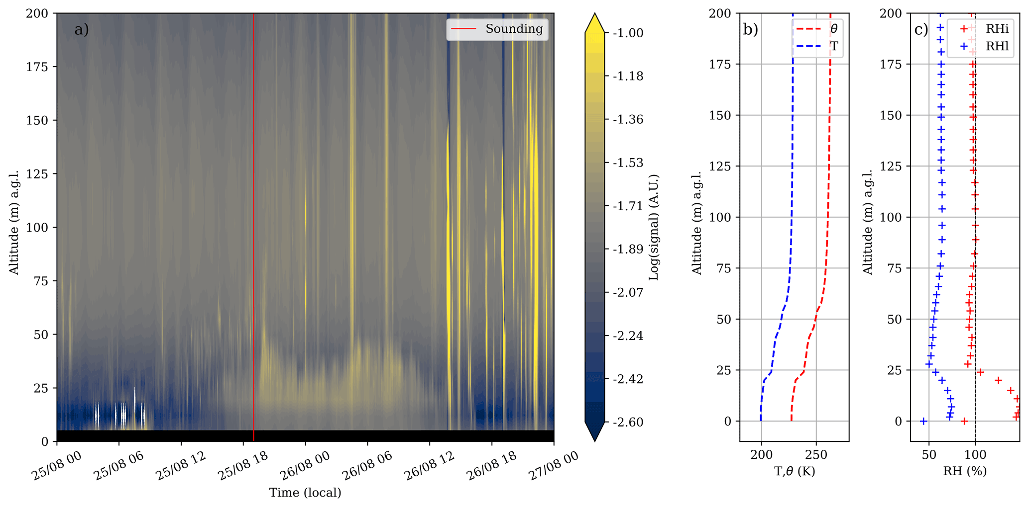
Figure 2(a) Time–height plot of the lidar backscattering signal intensity during the first fog event between 12:00 LT on 8 March to 00:00 LT on 10 March 2018. The red line indicates the radiosonde launching time. Panel (b) shows the vertical profile of temperature (blue) and potential temperature (calculated with a reference pressure of 105 Pa, red) from the radiosounding. The black arrow indicates the top of the boundary layer. Panel (c) shows the vertical profile of relative humidity with respect to ice (RHi, red) and with respect to liquid water (RHl, blue) from the same radiosounding.
3.1 Event 1: 7–9 March 2018
3.1.1 Overview
The first ice fog event we focus on occurred between 7 and 9 March 2018. A picture showing the landscape of Dome C in the shallow and thin fog during sunset on 8 March 2018 is shown in Fig. 1. Figure 2 shows a time–height plot of the lidar backscattering signal during the event. A clear shallow fog layer starts to develop from about 06:00 LT on 8 March and grows from the ground until it reaches a maximum height of 200 m at 01:00 LT on 9 March. Its depth then sharply decreases until 06:00 LT, and the decay continues until dissipation at 00:00 LT on 10 March.
The radiosounding reveals a layer supersaturated with respect to ice from 40 to 150 m a.g.l. The maximum RHi value of 113 % is reached at 130 m a.g.l. which roughly corresponds to the upper limit of the fog layer and of the boundary-layer top inversion at this time. The temperature between the ground and 120 m ranges between 216 K at the bottom and 230 K at the top (Fig. 2b), which confirms that the fog develops in cirrus-like temperature conditions.
The 3 m wind slightly veers from a southwesterly to a southeasterly direction, and its magnitude increases throughout the event from 2 to 7.5 m s−1. Libois et al. (2014) identify drifting snow events at Dome C when the 10 m wind speed exceeds 7 m s−1. Assuming a logarithmic wind speed profile between the surface and 10 m and an aerodynamic roughness length value of 1 mm (Vignon et al., 2016), this corresponds to a 3 m wind speed threshold value of 3.5 m s−1. Note that at 22:00 LT on 7 March and after 06:00 LT on 8 March, the 3 m wind speed exceeds the threshold, and some snow drift is therefore possible during those periods.

Figure 3(a) The 2 d back trajectories ending at 50 (blue) and 100 m a.g.l. (red) at the four grid points closest to Dome C. Panels (b) and (c) show the time series of the wind speed and origin at three levels on the mast. The dashed red line in (b) indicates the 3 m wind speed threshold value for snowdrift triggering (see details in the main text). The grey band in (c) delimits the wind direction range in which the flow can possibly be affected by station exhaust. Black arrows indicate the times at which the fog visually appears and disappears near the surface in the lidar measurements.
As the air is coming from the southern sector, we do not expect this fog to be associated with an oceanic intrusion. It rather corresponds to a cloud that forms locally or slightly upstream over the Antarctic Plateau. This is confirmed by the analysis of air mass back trajectories arriving at 50 and 100 m a.g.l. shown in Fig. 3a. As the temperature along the trajectories never exceeds 235 K (not shown), an advection of supercooled liquid droplets towards Dome C is unlikely, which confirms that the fog does not have a liquid origin.
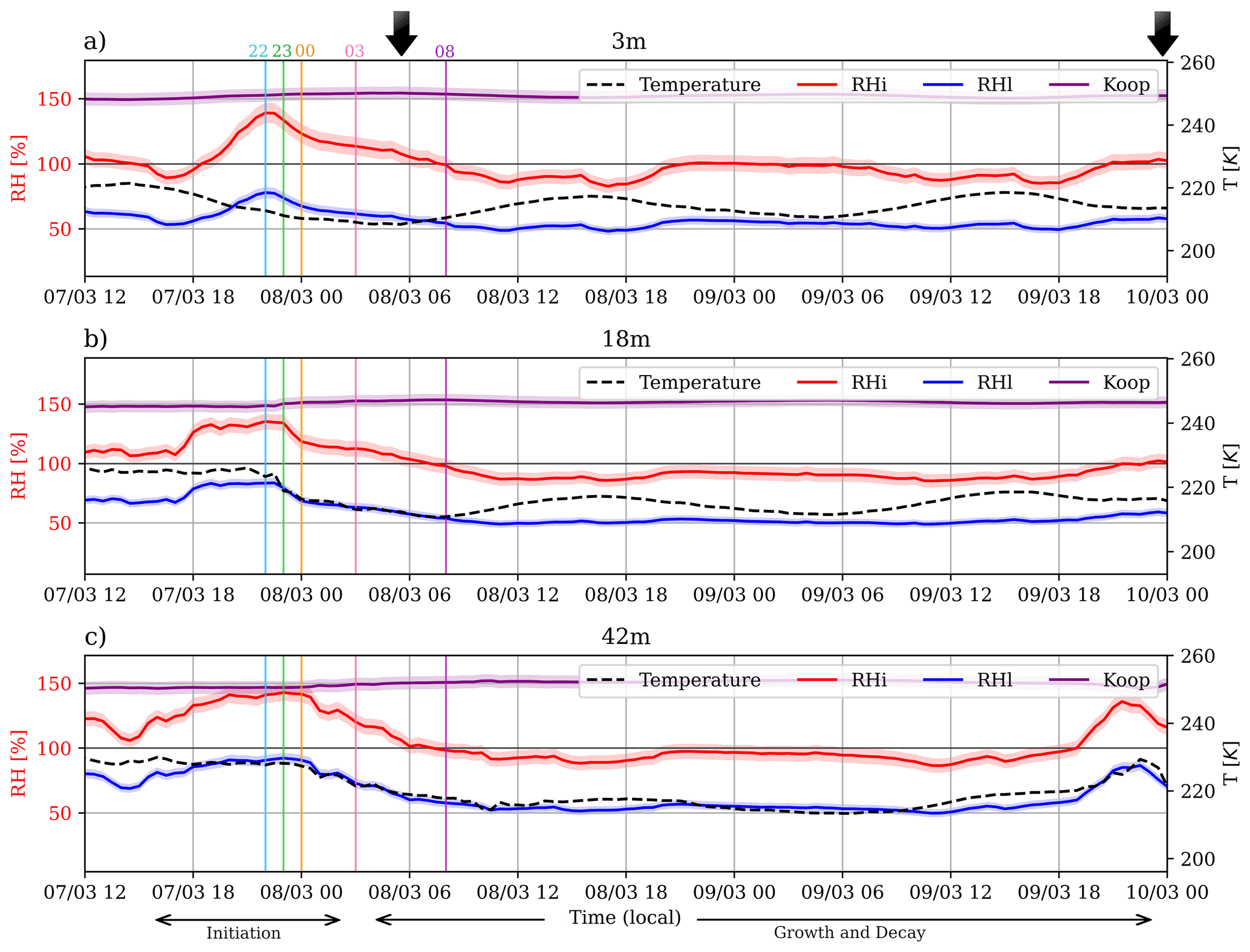
Figure 4Time series of the temperature (dashed black line) and relative humidity with respect to ice (RHi, solid red line) and liquid water (RHl, solid blue line) at 3 (a), 18 (b) and 42 m a.g.l. (c). The red and blue shading shows the RH uncertainty ranges as estimated in Appendix A. The purple line shows the homogeneous freezing RHi threshold value of Koop et al. (2000). The 100 % RH value is highlighted with a solid black line. Vertical coloured bars indicate the times at which vertical profiles are analysed in Fig. 5. Black arrows indicate the times at which the fog visually appears and disappears near the surface in the lidar measurements.
Temperature measurements on the mast remain below 235 K throughout the event, and one can notice a weak diurnal cycle at 3 m that is almost totally damped at 42 m (Fig. 4). A close investigation of the vertical profile of the potential temperature – very close to absolute temperature over the mast depth – reveals that the boundary layer transits between a weakly convective state during daytime to a stable state during nighttime. The fog does not have a clear radiative signature at the surface even though a slight decrease in downward longwave radiation is noticeable during the evening of 7 March (Fig. B2a), which concurs with the overall decrease in air temperature (Fig. 4).
3.1.2 Fog initiation: 15:00 LT, 7 March, to 03:00 LT, 8 March
We now focus on the initiation period from 15:00 LT on 7 March to 03:00 LT on 8 March. At the 42 m level, RHi first exhibits an increase from 106 % to 143 % which coincides with an increase in vapour partial pressure. At the 3 m level, a later but sharper increase in RHi up to 139 % at 22:00 LT on 7 March is noticeable, and unlike at 42 and 18 m, this increase is partly explained by a decrease in temperature during the day–night transition. The maximum RHi reached at the three levels ranges between 139 % and 143 %. RHl remains lower than 78 % at 3 m, but it exceeds 90 % at 42 m at 23:00 LT on 7 March.
RHi then gradually decreases and reaches 100 % at the three levels at 08:00 LT on 8 March (Fig. 4). The decrease starts at 22:30 LT on 7 March at the 3 m level, a half hour later at 18 m and 2 h later at 42 m.
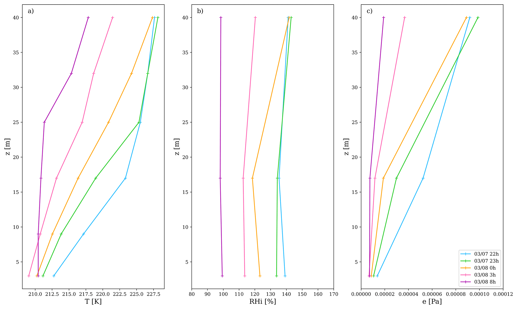
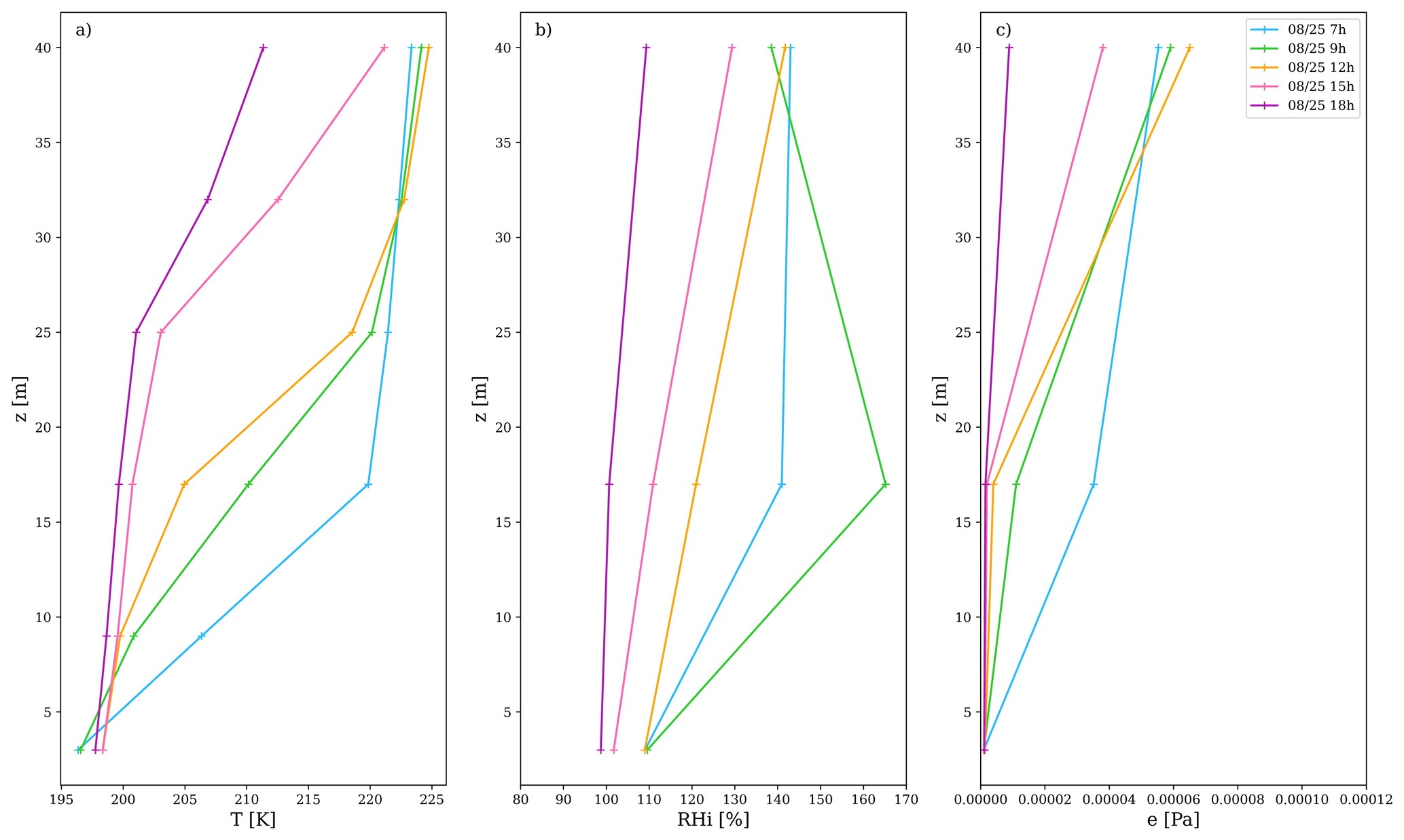
Figure 5Vertical profiles of temperature (a), relative humidity with respect to ice (b) and vapour partial pressure (c) at different times during the fog development phase.
Given the maximum RHl and RHi values attained, the aerosol deliquescence and solution droplet freezing at 3 m a.g.l. are not very likely, but their occurrence cannot be completely excluded since Baumgartner et al. (2022) show that homogeneous freezing can start at RHi values slightly lower than the Koop et al. (2000) threshold. As the station exhaust does not affect our measurements (see grey shading in Fig. 3c), the decrease in 3 m relative humidity from 22:00 LT can therefore be explained by (i) ice nucleation and vapour deposition onto newly formed ice crystals, by (ii) a net downward turbulent moisture flux towards the ground surface as the vertical gradient of vapour partial pressure is positive (see Fig. 5c), and/or by (iii) the vapour deposition of drifting ice crystals in the surface layer, although the erosion threshold is barely attained.
At 18 m, the decrease in RHi from 22:00 LT is co-incidental with a sharp decrease in vapour partial pressure, as well as a decrease in gradient of vapour partial pressure (Fig. 5c) between 3 and 18 m. The 18 m drying from 22:00 LT is therefore due to the turbulent mixing near the surface with a net flux of a moisture oriented downward.
At 42 m, a similar decrease in relative humidity and temperature is observed, but the particularity of this level, and probably that of the overlying air layers, is that RHi gets very close to the Koop et al. (2000) RHi threshold for homogeneous freezing of solution droplets in the middle of the night (see time series in Fig. 4c and how the system evolves in a RH–temperature space in Fig. B1). The difference between the RHi value and the homogeneous freezing threshold is even smaller than the measurement uncertainty (red shading in Fig. 4c). We can therefore assume that the ice fog forms a few tens of metres above the ground surface through homogeneous nucleation, and the subsequent decrease in RHi at 42 m is therefore partly explained by the vapour deposition onto newly formed ice crystals. A few patches of ice fogs are indeed noticeable during the night between 7 and 8 March (Fig. 2a).
3.1.3 Growth and decay: 03:00 LT, 8 March, to 23:00 LT, 9 March
From 03:00 to 08:00 LT on 8 March, the temperature vertical profile shows a clear night–day transition, i.e. a transition from an “exponential” shape characteristic of very stable boundary layers to a convective profile with a well-mixed layer capped by a shallow temperature inversion whose height further increases during the day (Fig. 5a). A close inspection of the vertical profile of specific humidity between 3 m and the surface at 08:00 LT (not shown) – assuming that the specific humidity at the snow surface equals the saturation-specific humidity at the surface temperature – reveals that the vertical gradient of specific humidity and subsequently the surface flux of water vapour reverse sign and become oriented upward. The supply of water vapour from the snow surface – and possibly of drifting ice crystals since the surface wind speed exceeds the erosion threshold (Fig. 3b) – can therefore deposit onto the ice crystal embryos nucleated in the early morning and make them grow and become visible in the lidar signal.
Figure 2a shows that the depth of the fog layer gradually increases from 06:00 LT on 8 March up to about 80 m at 18:00 LT on 8 March as the daytime convective boundary layer deepens in (Stull, 1990). The growth of the fog is possible in the higher part of the boundary layer as its top is supersaturated with respect to ice (Fig. 2c). Ice crystals can hence grow by vapour deposition and sediment down to the near-surface layers where they probably partly sublimate (Figs. 2 and 4). Concurring with Genthon et al. (2022b) (see their Fig. 8), the near-surface air becomes subsaturated with respect to ice particularly during daytime when the near-surface air warms by convective mixing. As night falls around 19:00 LT on 8 March, one can then note a sharper deepening of the fog up to 200 m. The mechanisms responsible for this sudden growth cannot be directly identified from our measurements, but one can nonetheless make some assumptions. As the wind speed increases in the late afternoon (Fig. 3b), one could expect an enhanced vertical mixing of ice particles, but a close examination of the wind speed profile from the radiosonde reveals a weak local wind shear at the top of the boundary layer. Nonetheless, in the late afternoon, the decrease in the shallow convection intensity leads to a decrease in the capping temperature inversion strength (Ricaud et al., 2012). The weak vertical gradient of temperature at the top of the evening convective boundary layer is visible in Fig. 2b (see black arrow), whereas a second higher and stronger temperature inversion is visible at the top of the fog layer and probably induced by the cloud-top radiative cooling. Izett and van de Wiel (2020) show that the growth of a radiative liquid fog layer can suddenly accelerate when the vertical gradient of temperature decreases (i.e. when the vertical gradient of saturation-specific humidity decreases; see their Eq. 7). If we assume a homogeneous freezing process, the ice nucleation occurs at the Koop et al. (2000) threshold; that is, according to an increasing function of temperature. Subsequently, we can reasonably think that the conceptual model of Izett and van de Wiel (2020) is qualitatively valid for the present ice fog event. We can therefore assume that during the evening of 8 March, the ice fog grows radiatively, and the depth of the layer sharply increases due to the decrease in the temperature vertical gradient. It is worth noting that the growth rate of the fog layer (about 120 m in 7 h from visual inspection in Fig. 2a, which is ≈17 m h−1) is quite similar to the growth rate of the radiative liquid fog portrayed in Izett and van de Wiel (2020) during the acceleration phase.
The fog grows until it reaches the top of the atmospheric layer supersaturated with respect to ice. From 18:00 LT on 8 March to 06:00 LT on 9 March, the RHi at the three levels is ≤100 % (Fig. 4) – in agreement with the radiosounding shown in Fig. 2c – while the lidar detects ice condensates from the surface up to 200 m a.g.l. The top height of the fog layer then drops down to about 50 m at 07:00 LT on 9 March and then slightly increases back at a time which corresponds to the deepening of the shallow-convective diurnal boundary layer. The fog layer then becomes shallower and shallower from 15:00 LT on 9 March as the turbulent mixing in the boundary layer weakens. The fog vanishes during the evening of 9 March, and RHi and temperature at 42 m increase up to their values before fog formation.
3.2 Event 2: 25–27 August 2018
3.2.1 Overview
The second case study occurred between 25 and 27 August 2018. No picture is available since the sun is almost always below the horizon during this period of the year. At 15:00 LT on 25 August a very shallow – about 20 m deep – ice fog starts to be visible in the lidar profiles (Fig. 6a). Its depth then oscillates between 25 and 50 m a.g.l., and the fog vanishes at around 14:00 LT on 26 August. This event is particularly interesting since its vertical extent is almost the same as the one of the meteorological mast. Note that highly reflective bands are observed during 26 August, and most of them correspond to diamond dust precipitation “peaks” falling from the mid-troposphere. The radiosounding reveals a supersaturated layer with respect to ice below 30 m a.g.l. with a maximum RHi value of 147 %. The relative humidity with respect to liquid water also exceeds 75 % near the surface (Fig. 6c).
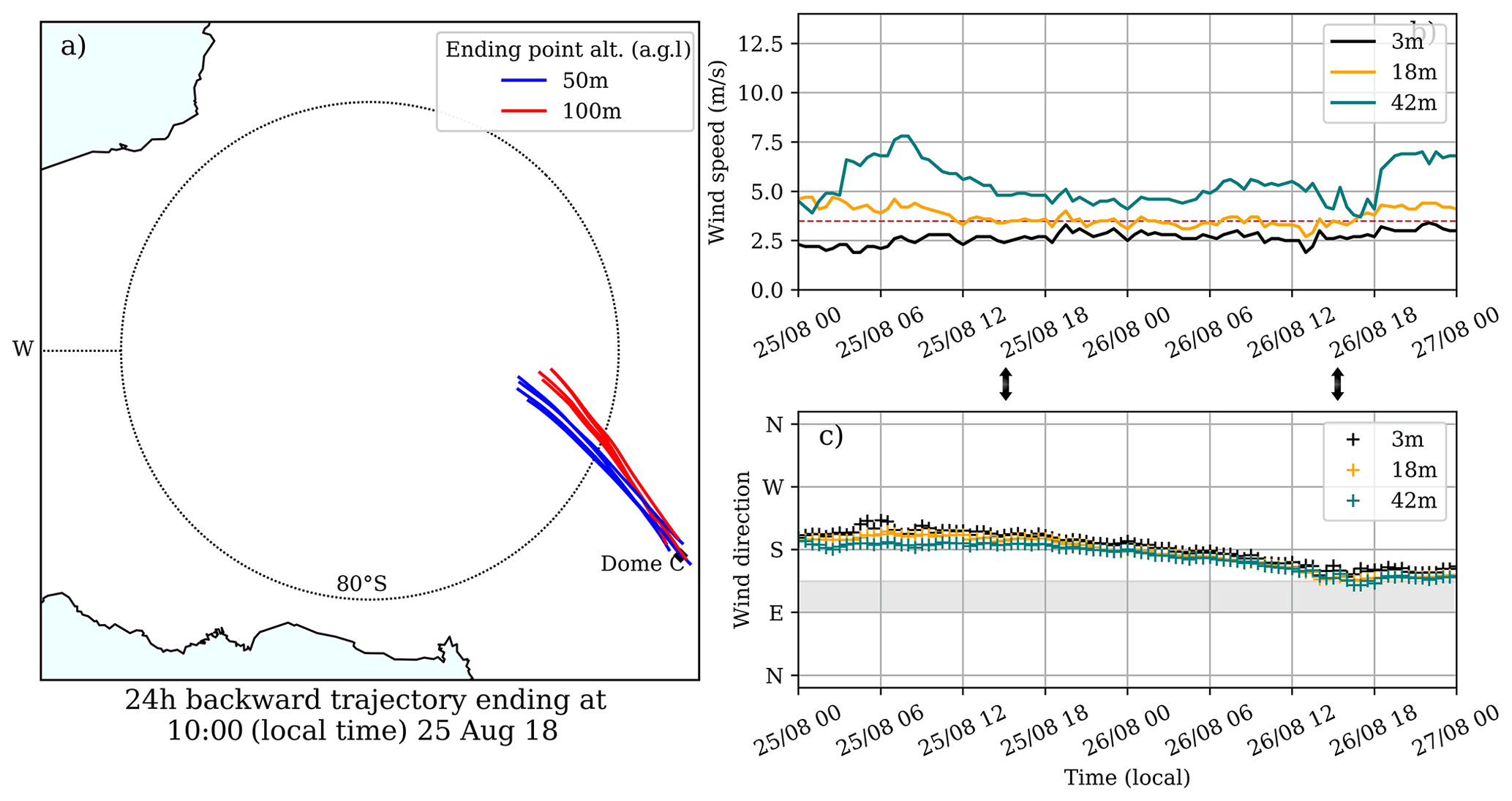
Figure 7Same as Fig. 3 but for Event 2.
Fig. 7b shows that the 3 m wind speed remains below 4 m s−1 throughout the event and never exceeds the threshold value to trigger drifting snow. Its direction slightly changes from southwesterly to a southeasterly, suggesting that the air parcels reaching Dome C come from the high Antarctic Plateau (Fig. 7b) and that our measurements are not affected by station exhaust except during the very end of the event (see grey shading in Fig. 7c). The back trajectories shown in Fig. 7a confirm the continental origin of the flow, and as the temperature measured at the station is much lower than 235 K, a liquid origin of the fog can be ruled out. The time series of observational data along the mast reveal a near-constant 3 m temperature of about 200 K during the event and confirm the absence of a diurnal cycle during this period of the year.
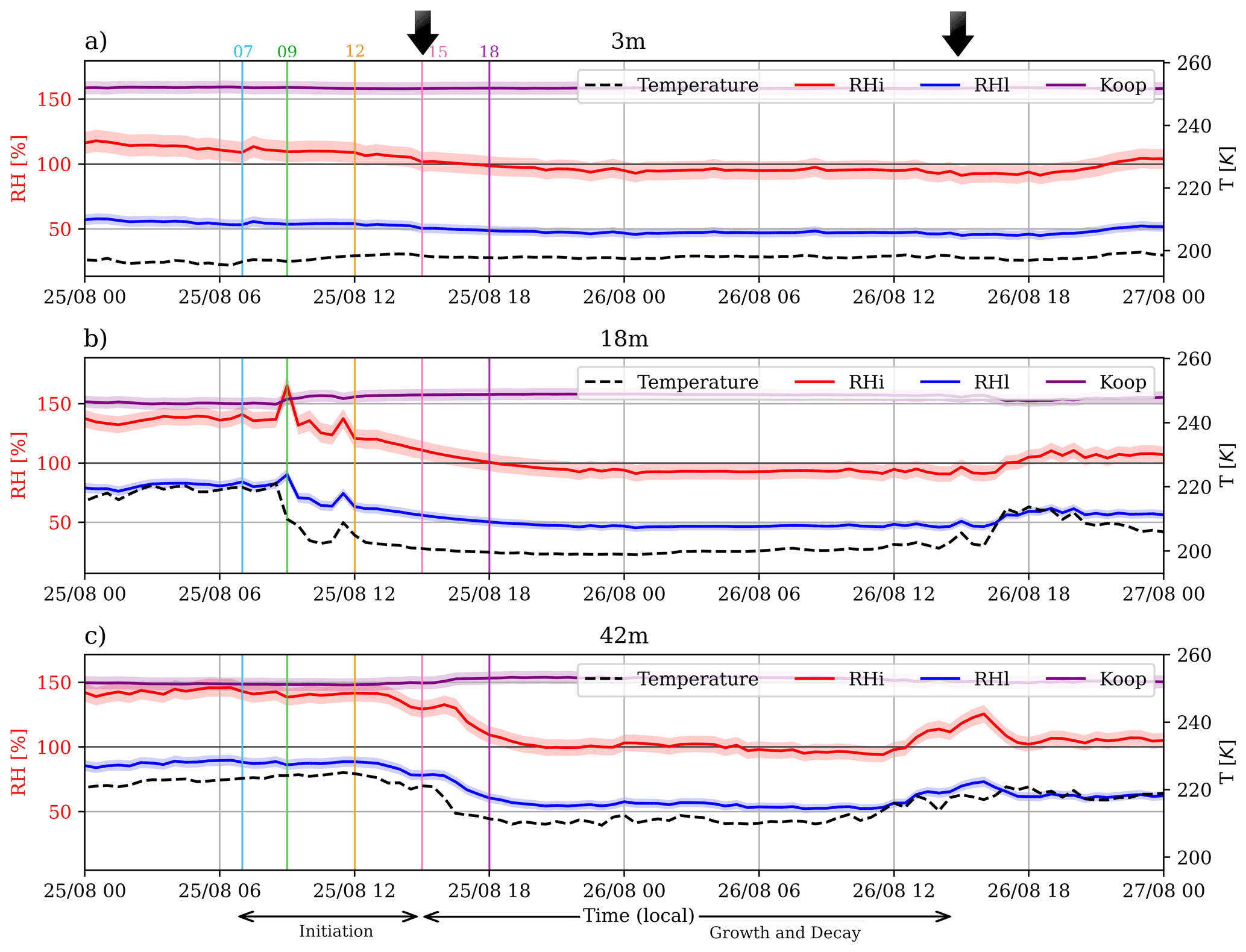
3.2.2 Fog initiation: 06:00 to 15:00 LT, 25 August
A significant drop in temperature at 09:00 LT is observed at 18 m. This cooling is due to an abrupt transition between a very stable to a weakly stable dynamical regime of the boundary layer (van de Wiel et al., 2017; Baas et al., 2019; van der Linden et al., 2019) driven by an increase in the synoptic wind speed (note that the wind at 42 m, i.e. at the top or above the shallow boundary layer, is a reasonable proxy of the synoptic wind; see Fig. 8c). Subsequently the temperature profile evolves from a typical “exponential” shape to a concave shape (Vignon et al., 2017) owing to a more vigorous turbulent transport of heat towards the surface (Fig. 9). At 18 m the cooling rate is particularly intense and equals 5 K h−1 between 08:00 and 11:00 LT on 25 August. As an analogy with typical air-parcel cooling within updraft in the middle and high troposphere, such a cooling rate roughly corresponds to an adiabatic air ascent of 0.10 m s−1.
At 42 m, RHi approaches the Koop et al. (2000) threshold between 04:00 and 05:00 LT on 25 August, and some preliminary crystal nucleation can already occur at this time. However at 09:00 LT on 25 August RHi at 18 m suddenly increases as temperature drops and clearly exceeds the Koop et al. (2000) homogeneous freezing threshold. RHl exceeds 90 % at the same time (see Figs. 8b and B1). The relative humidity does not substantially change at the two other levels at this time, leading to a well-marked maximum in the vertical profile (Fig. 9b). It is worth mentioning that Genthon et al. (2022b) show that the climatological RHi along the mast also exhibits a clear maximum at 18 m due to the non-linear dependence of relative humidity on temperature and atmospheric water content. Therefore, the initiation of the second fog event seems mainly due to a homogeneous freezing process starting between 3 and 42 m a.g.l. around 09:00 LT on 25 August. The density and size of ice crystals become sufficiently large to be well visible in the lidar signal a few hours later. From 10:00 LT on 25 August, RHi at 18 m starts a pronounced decrease due to the vapour deposition onto newly formed crystals and to a downward turbulent flux of water vapour as the vertical gradient of vapour partial pressure between 3 and 18 m is positive (Fig. 9c).
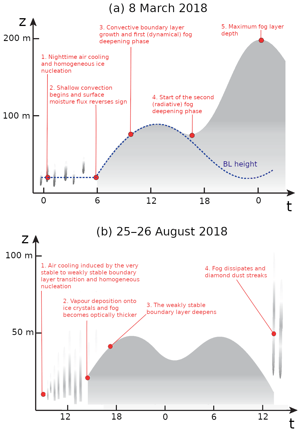
Figure 10Conceptual scheme of the formation and growth of the two ice fogs studied in the paper.
3.2.3 Growth and decay: 15:00 LT, 25 August, to 15:00 LT, 26 August
The decrease in RHi at 42 m occurs at 15:00 LT, and it coincides with a decrease in temperature associated with the deepening of the weakly stable boundary layer (Figs. 8c and 9a). The decrease in the 42 m RHi also concurs with the increase in fog layer depth visible in the lidar data between 15:00 and 18:00 LT on 25 August (Fig. 6a) and can therefore be attributed to the deposition of water vapour onto ice crystals. The saturation is reached at 19:00 LT on 25 August.
From the evening of 25 August, RHi remains close to but slightly below saturation at 3 and 18 m probably owing to a net flux of vapour towards the surface in the very shallow boundary layer. Ice crystals at these two heights can therefore not grow very close to the surface, but their detection at 18 m by the lidar may be rather explained by some sedimentation from higher layers.
At 12:00 LT on 26 August, the fog starts to dissipate from the top, and the air at 42 m becomes supersaturated with respect to ice (Fig. 8c). A few hours later a decrease in RHi back to saturation occurs probably due to vapour deposition onto the diamond dust precipitation streaks that suddenly fall down from the low and middle troposphere (Fig. 6a).
Temperature and humidity measurements from advanced thermo-hygrometers along a 45 m mast are combined with lidar and radiosonde observations and air-parcel back trajectories to study the development of two fog events at cirrus temperatures in the near-surface atmosphere of Dome C, high Antarctic Plateau. For both case studies, fog forms locally and does not correspond to warm maritime intrusions. Lidar observations evidenced shallow fogs, and the innovative moisture measurements along the tower allowed us to explain the mechanisms responsible for their formation.
Figure 10 summarises the development of the two fog events with two schematics. The values of supersaturation that are attained and the very low temperatures that prevent the pre-existence of supercooled liquid droplets suggest that the two ice fog clouds are initiated by the homogeneous freezing of solution aerosols in the stably stratified boundary layer. This study presents the first observational evidence that this process can be responsible for the formation of an ice fog. The highest supersaturations occur at a height where the air cools down by turbulent mixing and radiation and where the downward flux of water vapour is sufficiently weak. The evolution of the fog is thereby tightly related to the turbulent dynamics of the boundary layer which experiences a weak diurnal cycle in the first study case and a dynamical transition between a very stable and a weakly stable state in the second case.
Regarding the potential similarity between Antarctic ice fogs and cirrus clouds, this study suggests that the homogeneous freezing of solution particles, i.e. a common path to cirrus cloud formation, can be studied in natural conditions near the ground surface of the Antarctic Plateau. More generally, it emphasises that Dome C is a relevant place to carry out observational studies of microphysical processes in very cold ice clouds. Furthermore, the analysis of humidity measurements during the growing phase of fog gives access to the timescale at which the vapour is depleted, even though it is particularly delicate to disentangle the dynamical – i.e. turbulent mixing – from the microphysical – i.e. deposition onto ice crystals – causes. The development of the fogs is indeed tightly coupled with the dynamics of the boundary layer. This is a non-negligible difference with cirrus clouds in which ice crystal properties strongly depend on the dynamics of gravity waves (e.g. Jensen et al., 2016) and local turbulent eddies (e.g. Gultepe and Starr, 1995).
While the available observations at Dome C make it possible to characterise the overall development of ice fogs, they do not give direct information about the type – homogeneous or heterogeneous – of the ice nucleation process and do not allow for a fine understanding of the interactions between cloud microphysics, radiation and turbulent dynamics. Collecting sedimenting ice crystals during ice fog events and establishing formvar replicas thereof in the manner of Santachiara et al. (2016) would allow us to analyse the morphological structure of crystals and to perform chemical analyses of potentially remaining particles after sublimation. Running large-eddy simulation models with an advanced microphysical scheme for cold clouds and the capability of simulating the extreme boundary layer at Dome C (Couvreux et al., 2020) would also help us better understand the mechanisms driving the growth and decay of the ice fogs. Furthermore, investigating the frequency of occurrence of very cold ice fogs at Dome C was beyond the scope of this study. This aspect would deserve further attention in the future to figure out their climatological impacts on the Antarctic Plateau.
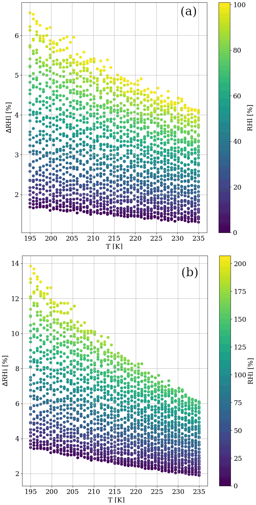
Figure A1Uncertainty in the RHl (a) and RHi (b) estimations as a function of temperature (x axis) and RHl and RHi (colour shading), respectively.
The estimation of RHl and RHi from the advanced thermo-hygrometers depends on Genthon et al. (2017) and Genthon et al. (2022b):
-
the measurement of the relative humidity with respect to liquid water in the heated inlet RHlh by the HMP155 probe;
-
the measurement of the temperature of the heated inlet Th by the HMP155 (PT-100);
-
the measurement of the ambient temperature T by the independent PT100 platinum resistance thermometer.
RHl and RHi are then calculated with the following expressions:
with esl and esi being the saturation water pressure with respect to liquid and ice, respectively, and calculated with the formulae of Murphy and Koop (2005). According to the manufacturers, the accuracy of the relative humidity measurement below −40 ∘C is of the reading in percentage, and the accuracy of the temperature measurement is . To estimate the uncertainties in the RHl and RHi end products, we perform a Monte Carlo test with 1000 uniform resamples of RHlh, Th and T in the interval (value − accuracy, value + accuracy). The uncertainties Δ RHl and Δ RHi are evaluated as 1 standard deviation of the obtained distributions for each bin of relative humidity and temperature. In the calculation, we assume that the air reaching the hygrometer sensor in the heated inlet is ≈5 K warmer than the ambient air (mean over the measurement period: 4.9 K; standard deviation: 0.7 K).
Panels a and b, respectively, in Fig. A1 show how the uncertainty in the RHl and RHi estimation depends on temperature. For each temperature bin on the x axis, the dependence is explored for different RHl and RHi values below liquid saturation (colour shading).
ΔRHl and ΔRHi can be expressed as continuous functions of relative humidity and temperature with a regression of the following form:
with a0l,i, a1l,i, a2l,i and a3l,i being the regression coefficients. The R2 coefficients of the regression equal 0.990 and 0.993 for ΔRHl and ΔRHi, respectively.
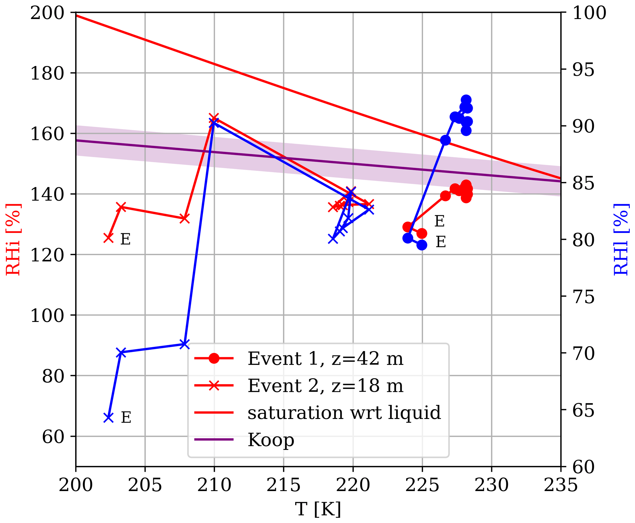
Figure B1RHi (red curves, left y axis) and RHl (blue curve, right y axis) evolution as a function of temperature at the level of nucleation during the initiation phase of the fog. Lines with circles refer to the first event (from 21:00 LT on 7 March to 02:00 LT on 8 March), while the lines with crosses refer to the second event (from 06:00 to 11:00 LT on 25 August). “E” indicates the endpoint. The solid red line shows RHi value at liquid water saturation and the purple line the Koop et al. (2000) homogeneous freezing RHi threshold value.
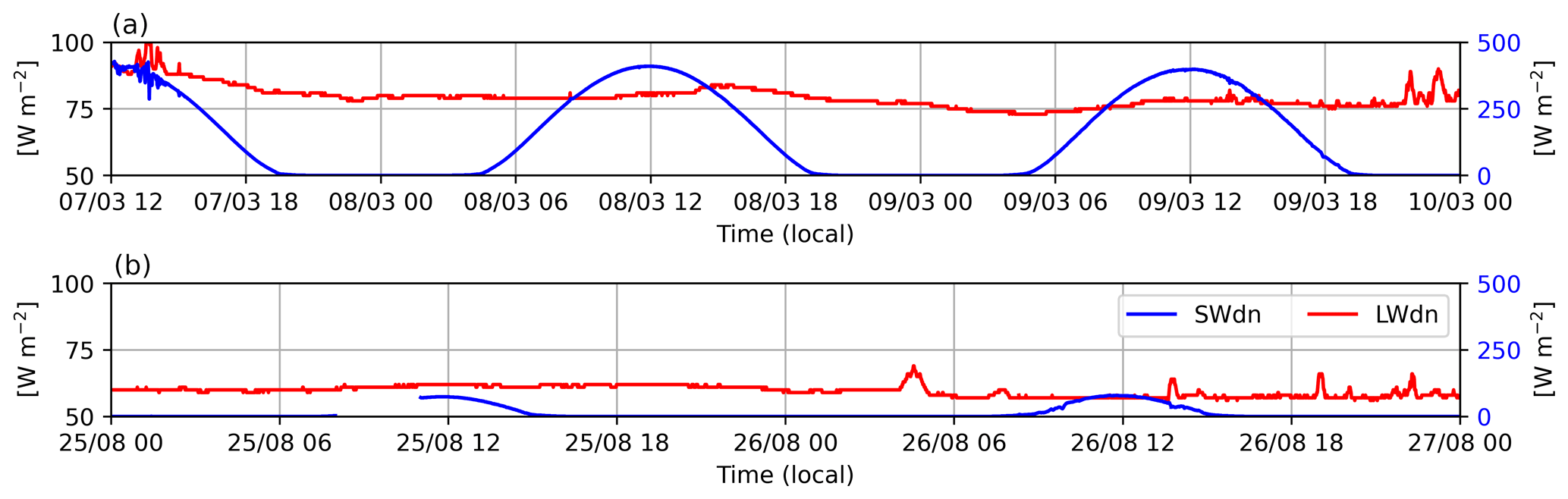
Figure B2Time series of downward longwave (LWdn, red) and shortwave (SWdn, blue) radiative fluxes at the surface during the first (a) and second (b) case studies.
The Dome C temperature, wind and humidity datasets used in this study are thoroughly described in Genthon et al. (2021c) (https://doi.org/10.5194/essd-13-5731-2021) and Genthon et al. (2022b) (https://doi.org/10.5194/essd-14-1571-2022) and distributed on PANGAEA (Genthon et al., 2021a; https://doi.org/10.1594/PANGAEA.932512; Genthon et al., 2021b; https://doi.org/10.1594/PANGAEA.932513; Genthon et al., 2022a; https://doi.org/10.1594/PANGAEA.939425). Radiosonde data are freely distributed at https://www.climantartide.it/ (Climantartide, 2002). The tropospheric depolarisation lidar data can be obtained at http://lidarmax.altervista.org/englidar/_AntarcticLIDAR.php (Del Guasta, 2008). BSRN data are available on PANGAEA at https://doi.org/10.1594/PANGAEA.880000 (Driemel et al., 2018b) (https://doi.org/10.5194/essd-10-1491-2018).
EV, LR and CG designed and conducted the study. LR and EV analysed the data, and LR made the figures. MDG collected and processed the lidar data. CG collected and maintained the meteorological measurements on the mast at Dome C. AJH, JBM and AB provided scientific expertise on cold microphysics and contributed to the results' interpretation. EV wrote the paper with contributions from all the authors.
The contact author has declared that none of the authors has any competing interests.
Publisher’s note: Copernicus Publications remains neutral with regard to jurisdictional claims in published maps and institutional affiliations.
We gratefully thank Roxanne Jacob for examining additional photographs during fog events at Dome C. This research was conducted in the framework of the CALVA 1013 and PRE-REC observation programmes with the support of the French polar institute (IPEV) and the Programma Nazionale di Ricerche in Antartide (PNRA). Radiosounding data have been acquired from the database of the IPEV/PNRA project “Routine Meteorological Observation at Station Concordia” https://www.climantartide.it/ (last access: 23 September 2022) with the help of Paolo Grigioni.
This project has received funding from the European Research Council (ERC) under the European Union’s Horizon 2020 research and innovation programme (grant no. 951596).
This paper was edited by Martina Krämer and reviewed by two anonymous referees.
Argentini, S., Pietroni, I., Mastrantonio, G., P., V. A., Dargaud, G., and Petenko, I.: Observations of near surface wind speed, temperature and radiative budget at Dome C, Antarctic Plateau during 2005, Antarct. Sci., 26, 104–112, https://doi.org/10.1017/S0954102013000382, 2014. a
Baas, P., van de Wiel, B. J. H., van Meijgaard, E., Vignon, E., Genthon, C., van der Linden, S. J. A., and de Roode, S. R.: Transitions in the wintertime near-surface temperature inversion at Dome C, Antarctica, Q. J. Roy. Meteorol. Soc., 145, 930–946, https://doi.org/10.1002/qj.3450, 2019. a
Baumgartner, M., Rolf, C., Grooß, J.-U., Schneider, J., Schorr, T., Möhler, O., Spichtinger, P., and Krämer, M.: New investigations on homogeneous ice nucleation: the effects of water activity and water saturation formulations, Atmos. Chem. Phys., 22, 65–91, https://doi.org/10.5194/acp-22-65-2022, 2022. a, b, c, d
Belosi, F., Santachiara, G., and Prodi, F.: Ice-forming nuclei in Antarctica: New and past measurements, Atmos. Res., 145–146, 105–111, https://doi.org/10.1016/j.atmosres.2014.03.030, 2014. a
Blanchet, J.-P. and Girard, E.: Water vapor-temperature feedback in the formation of continental Arctic air: its implication for climate, Sci. Total Environ., 160–161, 793–802, https://doi.org/10.1016/0048-9697(95)04412-T, 1995. a
Climantartide: Osservatorio Meteo-Climatologico Antartico, http://www.climantartide.it/ (last access: 3 April 2020), 2002. a
Couvreux, F., Bazile, E., Rodier, Q., Maronga, B., Matheou, G., Chinita, M. J., Edwards, J., van Stratum, B. J., van Heerwaarden, C. C., Huang, J., Moene, A. F., Cheng, A., Fuka, V., Basu, S., Bou-Zeid, E., Canut, G., and Vignon, É.: Intercomparison of large-eddy simulations of the Antarctic boundary layer for very stable stratification, Bound.-Lay. Meteorol., 176, 369–400, https://doi.org/10.1007/s10546-020-00539-4, 2020. a
Curry, J. A., Meyer, F. G., Radke, L. F., Brock, C. A., and Ebert, E. E.: Occurrence and characteristics of lower tropospheric ice crystals in the arctic, Int. J. Climatol., 10, 749–764, https://doi.org/10.1002/joc.3370100708, 1990. a
Del Guasta, M.: INO LIDAR in Antarctica, lidarmax [data set], http://lidarmax.altervista.org/englidar/_AntarcticLIDAR.php (last access: 3 April 2020), 2008. a
DeMott, P. J., Rogers, D. C., Kreidenweis, S. M., Chen, Y., Twohy, C. H., Baumgardner, D., Heymsfield, A. J., and Chan, K. R.: The role of heterogeneous freezing nucleation in upper tropospheric clouds: Inferences from SUCCESS, Geophys. Res. Lett., 25, 1387–1390, https://doi.org/10.1029/97GL03779, 1998. a
Driemel, A., Augustine, J., Behrens, K., Colle, S., Cox, C., Cuevas-Agulló, E., Denn, F. M., Duprat, T., Fukuda, M., Grobe, H., Haeffelin, M., Hodges, G., Hyett, N., Ijima, O., Kallis, A., Knap, W., Kustov, V., Long, C. N., Longenecker, D., Lupi, A., Maturilli, M., Mimouni, M., Ntsangwane, L., Ogihara, H., Olano, X., Olefs, M., Omori, M., Passamani, L., Pereira, E. B., Schmithüsen, H., Schumacher, S., Sieger, R., Tamlyn, J., Vogt, R., Vuilleumier, L., Xia, X., Ohmura, A., and König-Langlo, G.: Baseline Surface Radiation Network (BSRN): structure and data description (1992–2017), Earth Syst. Sci. Data, 10, 1491–1501, https://doi.org/10.5194/essd-10-1491-2018, 2018a. a
Driemel, A., Augustine, J., Behrens, K., Colle, S., Cox, C., Cuevas-Agulló, E., Denn, F. M., Duprat, T., Fukuda, M., Grobe, H., Haeffelin, M., Hodges, G., Hyett, N., Ijima, O., Kallis, A., Knap, W., Kustov, V., Long, C. N., Longenecker, D., Lupi, A., Maturilli, M., Mimouni, M., Ntsangwane, L., Ogihara, H., Olano, X., Olefs, M., Omori, M., Passamani, L., Pereira, E. B., Schmithüsen, H., Schumacher, S., Sieger, R., Tamlyn, J., Vogt, R., Vuilleumier, L., Xia, X., Ohmura, A., and König-Langlo, G.: Baseline Surface Radiation Network (BSRN): structure and data description (1992–2017), Earth Syst. Sci. Data, 10, 1491–1501, https://doi.org/10.5194/essd-10-1491-2018, data available at: https://doi.org/10.1594/PANGAEA.880000, 2018b. a
Genthon, C., Six, D., Gallée, H., Grigioni, P., and Pellegrini, A.: Two years of atmospheric boundary layer observations on a 45-m tower at Dome C on the Antarctic Plateau, J. Geophys. Res. Atmos., 118, D05104, https://doi.org/10.1002/jgrd.50128, 2013. a
Genthon, C., Veron, D., Vignon, E., Six, D., Dufresne, J. L., Madeleine, J.-B., Sultan, E., and Forget, F.: Ten years of wind speed observation on a 45-m tower at Dome C, East Antarctic plateau, PANGAEA [data set], https://doi.org/10.1594/PANGAEA.932513, 2021a. a
Genthon, C., Veron, D., Vignon, E., Six, D., Dufresne, J. L., Madeleine, J.-B., Sultan, E., Forget, F.: Ten years of shielded ventilated atmospheric temperature observation on a 45-m tower at Dome C, East Antarctic plateau, PANGAEA [data set], https://doi.org/10.1594/PANGAEA.932512, 2021b. a
Genthon, C., Veron, D., Vignon, E., Six, D., Dufresne, J.-L., Madeleine, J.-B., Sultan, E., and Forget, F.: 10 years of temperature and wind observation on a 45 m tower at Dome C, East Antarctic plateau, Earth Syst. Sci. Data, 13, 5731–5746, https://doi.org/10.5194/essd-13-5731-2021, 2021c. a, b, c
Genthon, C., Veron, D., Vignon, E., Madeleine, J.-B., and Piard, L.: Water vapor observation in the lower atmospheric boundary layer at Dome C, East Antarctic plateau, PANGAEA [data set], https://doi.org/10.1594/PANGAEA.939425, 2022a. a
Genthon, C., Veron, D. E., Vignon, E., Madeleine, J.-B., and Piard, L.: Water vapor in cold and clean atmosphere: a 3-year data set in the boundary layer of Dome C, East Antarctic Plateau, Earth Syst. Sci. Data, 14, 1571–1580, https://doi.org/10.5194/essd-14-1571-2022, 2022b. a, b, c, d, e, f, g
Genthon, C., Piard, L., Vignon, E., Madeleine, J.-B., Casado, M., and Gallée, H.: Atmospheric moisture supersaturation in the near-surface atmosphere at Dome C, Antarctic Plateau, Atmos. Chem. Phys., 17, 691–704, https://doi.org/10.5194/acp-17-691-2017, 2017. a, b, c, d, e, f
Girard, E. and Blanchet, J.-P.: Simulation of Arctic Diamond Dust, Ice Fog, and Thin Stratus Using an Explicit Aerosol–Cloud–Radiation Model, J. Atmos. Sci., 58, 1199–1221, https://doi.org/10.1175/1520-0469(2001)058<1199:SOADDI>2.0.CO;2, 2001. a, b
Gultepe, I. and Starr, D. O.: Dynamical Structure and Turbulence in Cirrus Clouds: Aircraft Observations during FIRE, J. Atmos. Sci., 52, 4159–4182, https://doi.org/10.1175/1520-0469(1995)052<4159:DSATIC>2.0.CO;2, 1995. a
Gultepe, I., Zhou, B., Milbrandt, J., Bott, A., Li, Y., Heymsfield, A., Ferrier, B., Ware, R., Pavolonis, M., Kuhn, T., Gurka, J., Liu, P., and Cermak, J.: A review on ice fog measurements and modeling, Atmos. Res., 151, 2–19, https://doi.org/10.1016/j.atmosres.2014.04.014, 2015. a
Gultepe, I., Heymsfield, A. J., Gallagher, M., Ickes, L., and Baumgardner, D.: Ice Fog: The Current State of Knowledge and Future Challenges, Meteorol. Monograph., 58, 4.1–4.24, https://doi.org/10.1175/AMSMONOGRAPHS-D-17-0002.1, 2017. a, b
Heymsfield, A. J. and Sabin, R. M.: Cirrus Crystal Nucleation by Homogeneous Freezing of Solution Droplets, J. Atmos. Sci., 46, 2252–2264, https://doi.org/10.1175/1520-0469(1989)046<2252:CCNBHF>2.0.CO;2, 1989. a
Heymsfield, A. J., Krämer, M., Luebke, A., Brown, P., Cziczo, D. J., Franklin, C., Lawson, P., Lohmann, U., McFarquhar, G., Ulanowski, Z., and Tricht, K. V.: Cirrus Clouds, Meteorol. Monograph., 58, 2.1–2.26, https://doi.org/10.1175/AMSMONOGRAPHS-D-16-0010.1, 2017. a
Izett, J. G. and van de Wiel, B. J. H.: Why Does Fog Deepen? An Analytical Perspective, Atmosphere, 11, 8, https://doi.org/10.3390/atmos11080865, 2020. a, b, c
Jensen, E. J., Ueyama, R., Pfister, L., Bui, T. V., Alexander, M. J., Podglajen, A., Hertzog, A., Woods, S., Lawson, R. P., Kim, J.-E., and Schoeberl, M. R.: High-frequency gravity waves and homogeneous ice nucleation in tropical tropopause layer cirrus, Geophys. Res. Lett., 43, 6629–6635, https://doi.org/10.1002/2016GL069426, 2016. a
Kärcher, B. and Burkhardt, U.: A cirrus cloud scheme for general circulation models, Q. J. Roy. Meteorol. Soc., 134, 1439–1461, https://doi.org/10.1002/qj.301, 2008. a
Kärcher, B. and Lohmann, U.: A parameterization of cirrus cloud formation: Heterogeneous freezing, J. Geophys. Res.-Atmos., 108, D14, https://doi.org/10.1029/2002JD003220, 2003. a
Kikuchi, K.: Observations of Concentration of Ice Nuclei at Syowa Station, Antarctica, Journal of the Meteorological Society of Japan. Ser. II, 49, 20–31, https://doi.org/10.2151/jmsj1965.49.1_20, 1971. a
Kikuchi, K.: Sintering Phenomenon of Frozen Cloud Particles Observed at Syowa Station, Antarctica, Journal of the Meteorological Society of Japan. Ser. II, 50, 131–135, https://doi.org/10.2151/jmsj1965.50.2_131, 1972. a
Koop, T., Luo, B., Tsias, A., and Peter, T.: Water activity as the determinant for homogeneous ice nucleation in aqueous solutions, Nature, 406, 611–614, 2000. a, b, c, d, e, f, g, h, i, j, k
Lanconelli, C., Busetto, M., Dutton, E. G., König-Langlo, G., Maturilli, M., Sieger, R., Vitale, V., and Yamanouchi, T.: Polar baseline surface radiation measurements during the International Polar Year 2007–2009, Earth Syst. Sci. Data, 3, 1–8, https://doi.org/10.5194/essd-3-1-2011, 2011. a
Libois, Q., Picard, G., Arnaud, L., Morin, S., and Brun, E.: Modeling the impact of snow drift on the decameter-scale variability of snow properties on the Antarctic Plateau, J. Geophys. Res.-Atmos., 119, 662–681, https://doi.org/10.1002/2014JD022361, 2014. a, b
Marcolli, C.: Deposition nucleation viewed as homogeneous or immersion freezing in pores and cavities, Atmos. Chem. Phys., 14, 2071–2104, https://doi.org/10.5194/acp-14-2071-2014, 2014. a
Murphy, D. M. and Koop, T.: Review of the vapour pressures of ice and supercooled water for atmospheric applications, Q. J. Roy. Meteorol. Soc., 131, 1539–1565, https://doi.org/10.1256/qj.04.94, 2005. a, b
Nachbar, M., Duft, D., and Leisner, T.: The vapor pressure of liquid and solid water phases at conditions relevant to the atmosphere, J. Chem. Phys., 151, 064504, https://doi.org/10.1063/1.5100364, 2019. a
Neis, P., Smit, H. G. J., Krämer, M., Spelten, N., and Petzold, A.: Evaluation of the MOZAIC Capacitive Hygrometer during the airborne field study CIRRUS-III, Atmos. Meas. Tech., 8, 1233–1243, https://doi.org/10.5194/amt-8-1233-2015, 2015. a
Palchetti, L., Bianchini, G., Natale, G. D., and Guasta, M. D.: Far-Infrared Radiative Properties of Water Vapor and Clouds in Antarctica, Bull. Am. Meteorol. Soc., 96, 1505–1518, https://doi.org/10.1175/BAMS-D-13-00286.1, 2015. a
Ren, C. and Mackenzie, A. R.: Cirrus parametrization and the role of ice nuclei, Q. J. Roy. Meteorol. Soc., 131, 1585–1605, https://doi.org/10.1256/qj.04.126, 2005. a
Ricaud, P., Genthon, C., Durand, P., Attié, J., Carminati, F., Canut, G., Vanacker, J., Moggio, L., Courcoux, Y., Pellegrini, A., and Rose, T.: Summer to winter diurnal variabilities of temperature and water vapour in the lowermost troposphere as observed by HAMSTRAD over Dome C, Antarctica, Bound.-Lay. Meteorol., 143, 227–259, 2012. a
Ricaud, P., Bazile, E., del Guasta, M., Lanconelli, C., Grigioni, P., and Mahjoub, A.: Genesis of diamond dust, ice fog and thick cloud episodes observed and modelled above Dome C, Antarctica, Atmos. Chem. Phys., 17, 5221–5237, https://doi.org/10.5194/acp-17-5221-2017, 2017. a
Ricaud, P., Del Guasta, M., Bazile, E., Azouz, N., Lupi, A., Durand, P., Attié, J.-L., Veron, D., Guidard, V., and Grigioni, P.: Supercooled liquid water cloud observed, analysed, and modelled at the top of the planetary boundary layer above Dome C, Antarctica, Atmos. Chem. Phys., 20, 4167–4191, https://doi.org/10.5194/acp-20-4167-2020, 2020. a, b
Rowe, P. M., Walden, V. P., Brandt, R. E., Town, M. S., Hudson, S. R., and Neshyba, S.: Evaluation of Temperature-Dependent Complex Refractive Indices of Supercooled Liquid Water Using Downwelling Radiance and In-Situ Cloud Measurements at South Pole, J. Geophys. Res.-Atmos., 127, e2021JD035182, https://doi.org/10.1029/2021JD035182, 2022. a
Santachiara, G., Belosi, F., and Prodi, F.: Ice crystal precipitation at Dome C site (East Antarctica), Atmos. Res., 167, 108–117, https://doi.org/10.1016/j.atmosres.2015.08.006, 2016. a, b
Silber, I., Fridlind, A. M., Verlinde, J., Ackerman, A. S., Chen, Y.-S., Bromwich, D. H., Wang, S.-H., Cadeddu, M., and Eloranta, E. W.: Persistent Supercooled Drizzle at Temperatures Below −25 ∘C Observed at McMurdo Station, Antarctica, J. Geophys. Res.-Atmos., 124, 10878–10895, https://doi.org/10.1029/2019JD030882, 2019. a
Stull, R. B.: An Introduction to Boundary Layer Meteorology, Kluwer Academic Publishers, Dordrecht, Netherlands, 13, 670 pp., ISBN 9789400930278, 1990. a
Tomasi, C., Petkov, B. H., and Benedetti, E.: Annual cycles of pressure, temperature, absolute humidity and precipitable water from the radiosoundings performed at Dome C, Antarctica, over the 2005–2009 period, Antarctic Science, 24, 637–658, https://doi.org/10.1017/S0954102012000405, 2012. a, b
van der Linden, S. J., Edwards, J. M., van Heerwaarden, C. C., Vignon, E., Genthon, C., Petenko, I., Baas, P., Jonker, H. J., and van de Wiel, B. J.: Large-eddy simulations of the steady wintertime Antarctic boundary layer, Bound.-Lay. Meteorol., 173, 165–192, https://doi.org/10.1007/s10546-019-00461-4, 2019. a
van de Wiel, B. J. H., Vignon, E., Baas, P., van Hooijdonk, I. G. S., van der Linden, S. J. A., van Hooft, J. A., Bosveld, F. C., de Roode, S. R., Moene, A. F., and Genthon, C.: Regime transition in near-surface temperature inversions: a conceptual model, J. Atmos. Sci., 74, 1057–1073, https://doi.org/10.1175/JAS-D-16-0180.1, 2017. a
Vignon, E., Genthon, C., Barral, H., Amory, C., Picard, G., Gallée, H., Casasanta, G., and Argentini, S.: Momentum and heat flux parametrization at Dome C, Antarctica: a sensitivity study, Bound.-Lay. Meteorol., 162, 341–367, https://doi.org/10.1007/s10546-016-0192-3, 2016. a
Vignon, E., van de Wiel, B. J. H., van Hooijdonk, I. G. S., Genthon, C., van der Linden, S. J. A., van Hooft, J. A., Baas, P., Maurel, W., Traullé, O., and Casasanta, G.: Stable Boundary Layer regimes at Dome C, Antarctica: observation and analysis, Q. J. Roy. Meteorol. Soc., 143, 1241–1253, https://doi.org/10.1002/qj.2998, 2017. a, b
- Abstract
- Introduction
- Data and methods
- Results and discussion
- Summary and conclusions
- Appendix A: Uncertainties of relative humidity measurements
- Appendix B: Additional figures
- Data availability
- Author contributions
- Competing interests
- Disclaimer
- Acknowledgements
- Financial support
- Review statement
- References