the Creative Commons Attribution 4.0 License.
the Creative Commons Attribution 4.0 License.
 | 30 Aug 2022
Polar stratospheric nitric acid depletion surveyed from a decadal dataset of IASI total columns
Catherine Wespes
Gaetane Ronsmans
Lieven Clarisse
Susan Solomon
Daniel Hurtmans
Cathy Clerbaux
Pierre-François Coheur
In this paper, we exploit the first 10-year data record (2008–2017) of nitric acid (HNO3) total columns measured by the IASI-A/MetOp infrared sounder, characterized by an exceptional daily sampling and a good vertical sensitivity in the lower-to-mid stratosphere (around 50 hPa), to monitor the relationship between the temperature decrease and the observed HNO3 loss that occurs each year in the Antarctic stratosphere during the polar night. Since the HNO3 depletion results from the formation of polar stratospheric clouds (PSCs), which trigger the development of the ozone (O3) hole, its continuous monitoring is of high importance. We verify here, from the 10-year time evolution of HNO3 together with temperature (taken from reanalysis at 50 hPa), the recurrence of specific regimes in the annual cycle of IASI HNO3 and identify (for each year) the day and the 50 hPa temperature (“drop temperature”) corresponding to the onset of strong HNO3 depletion in the Antarctic winter. Although the measured HNO3 total column does not allow for the uptake of HNO3 by different types of PSC particles along the vertical profile to be differentiated, an average drop temperature of 194.2 ± 3.8 K, close to the nitric acid trihydrate (NAT) existence threshold (∼ 195 K at 50 hPa), is found in the region of potential vorticity lower than −10 × 10−5 (similar to the 70–90∘ S equivalent latitude region during winter). The spatial distribution and interannual variability of the drop temperature are investigated and discussed. This paper highlights the capability of the IASI sounder to monitor the evolution of polar stratospheric HNO3, a key player in the processes involved in the depletion of stratospheric O3.
- Article
(9835 KB) - Full-text XML
- BibTeX
- EndNote


The cold and isolated air masses found within the polar vortex during winter are associated with a strong denitrification of the stratosphere due to the formation of polar stratospheric clouds (PSCs, composed of nitric acid, HNO3; sulfuric acid, H2SO4; and water ice, H2O) (e.g., Peter, 1997; Voigt et al., 2000; von König, 2002; Schreiner et al., 2003; Peter and Grooß, 2012). These clouds strongly affect the polar chemistry by (i) acting as surfaces for the heterogeneous activation of chlorine and bromine compounds, in turn leading to enhanced O3 destruction (e.g., Solomon, 1999; Wang and Michelangeli, 2006; Harris et al., 2010; Wegner et al., 2012), and by (ii) removing gas-phase HNO3 temporarily or permanently through uptake by PSCs and sedimentation of large PSC particles to lower altitudes. The denitrification of the polar stratosphere during winter delays the reformation of ClONO2, a chlorine reservoir, and hence intensifies the O3 hole (e.g., Solomon, 1999; Harris et al., 2010; Tritscher et al., 2021). The heterogeneous reaction rates on PSC surfaces and the uptake of HNO3 strongly depend on the temperature and on the PSC particle type. The PSCs are classified into three different types based on their composition and optical properties: type Ia solid nitric acid trihydrate (NAT, HNO3⋅(H2O)3), type Ib liquid supercooled ternary solution (STS, HNO3/H2SO4/H2O with variable composition) and type II crystalline water ice particles (likely composed of a combination of different chemical phases) (e.g., Toon et al., 1986; Koop et al., 2000; Voigt et al., 2000; Lowe and MacKenzie, 2008). In the stratosphere, they mostly consist of mixtures of liquid and solid (STS and NAT) particles in varying number densities, with HNO3 being the major constituent of these particles. The large-sized NAT particles of low number density are the principal cause of sedimentation (Lambert et al., 2012, 2016; Pitts et al., 2013; Molleker et al., 2014). The formation temperature of STS (TSTS) and the thermodynamic equilibrium temperatures of NAT (TNAT) and ice (Tice) have been determined, respectively, as ∼ 192 K (Carslaw et al., 1995), ∼ 195.7 K (Hanson and Mauersberger, 1988) and ∼ 188 K (Murphy and Koop, 2005) for typical 50 hPa atmospheric conditions (5 ppmv H2O and 10 ppbv HNO3). While the NAT nucleation was thought to require pre-existing ice nuclei, i.e., temperatures below Tice (e.g., Zondlo et al., 2000; Voigt et al., 2003), recent observational and modeling studies have shown that HNO3 starts to condense in the early PSC season in liquid NAT mixtures well above Tice (∼ 4 K below TNAT, close to TSTS) even after a very short temperature threshold exposure (TTE) to these temperatures but also slightly below TNAT after a long TTE, whereas the NAT existence persists up to TNAT (Pitts et al., 2013; Hoyle et al., 2013; Lambert et al., 2016; Pitts et al., 2018). It has been recently proposed that the higher temperature condensation results from heterogeneous nucleation of NAT on meteoritic dust in liquid aerosol (Voigt et al., 2005; Hoyle et al., 2013; Grooß et al., 2014; James et al., 2018; Tritscher et al., 2021). Further cooling below TSTS and Tice leads to nucleation of liquid STS, of solid NAT onto ice and of ice particles mainly from STS (type II PSCs) (Lowe and MacKenzie, 2008). The formation of NAT and ice has also been shown to be triggered by stratospheric mountain waves (Carslaw et al., 1998; Hoffmann et al., 2017). Although the formation mechanisms and composition of STS droplets in stratospheric conditions are well described (Toon et al., 1986; Carslaw et al., 1995; Lowe and MacKenzie, 2008), the NAT and ice nucleation processes still require further investigation (Tritscher et al., 2021). This could be important as the chemistry–climate models (CCMs) generally oversimplify the heterogeneous nucleation schemes for PSC formation (Zhu et al., 2015; Spang et al., 2018; Snels et al., 2019), preventing an accurate estimation of O3 levels.
Over the last few decades, several satellite instruments have measured stratospheric HNO3 (e.g., MLS/UARS, Santee et al., 1999; MLS/Aura, Santee et al., 2007; MIPAS/ENVISAT, Piccolo and Dudhia, 2007; ACE-FTS/SCISAT, Sheese et al., 2017; SMR/Odin, Urban et al., 2009). Spaceborne instruments such as the CALIOP/CALIPSO lidar and MIPAS/Envisat measuring in the infrared are capable of detecting and classifying PSC types, allowing their formation mechanisms to be investigated (Lambert et al., 2016; Pitts et al., 2018; Spang et al., 2018, Tritscher et al., 2021, and references therein); these satellite data complement in situ measurements (Voigt et al., 2005) and ground-based lidar (Snels et al., 2019). From these available observational datasets, HNO3 depletion has been linked to PSC formation and detected below the TNAT threshold (Santee et al., 1999; Urban et al., 2009; Lambert et al., 2016; Ronsmans et al., 2018), but its relationship to PSCs still needs further investigation given the complexity of the nucleation mechanisms that depend on several parameters (e.g., atmospheric temperature, water and HNO3 vapor pressure, time exposure to temperatures, temperature history).
In contrast to the limb satellite instruments mentioned above, the infrared nadir sounder IASI offers a dense spatial sampling of the entire globe, twice a day (Sect. 2). While it cannot provide a vertical profile of HNO3 similar to that from the limb sounders, IASI provides reliable total column measurements of HNO3 characterized by a maximum sensitivity in the lower middle stratosphere around 50 hPa (20 km) during the dark Antarctic winter (Ronsmans et al., 2016, 2018) where PSCs form (Voigt et al., 2005; Lambert et al., 2012; Spang et al., 2016, 2018). This study aims to explore the 10-year continuous HNO3 measurements from IASI to provide a long-term global picture of depletion and of its dependence on temperatures during polar winter (Sect. 3). The temperature corresponding to the onset of the strong depletion in HNO3 records (here referred to as “drop temperature”) is identified in Sect. 4 for each observed year and discussed in the context of previous studies.
The HNO3 data used in the present study are obtained from measurements of the Infrared Atmospheric Sounding Interferometer (IASI) onboard the MetOp-A satellite. IASI measures the radiation of the Earth and the atmosphere in the thermal infrared spectral range (645–2760 cm−1), with a 0.5 cm−1 apodized resolution and low radiometric noise (Clerbaux et al., 2009; Hilton et al., 2012). Thanks to its polar sun-synchronous orbit with more than 14 orbits a day and a field of view of four simultaneous footprints of 12 km at nadir, IASI provides global coverage twice a day (9.30 AM and PM mean local solar time). That extensive spatial and temporal sampling in the polar regions is key to this study.
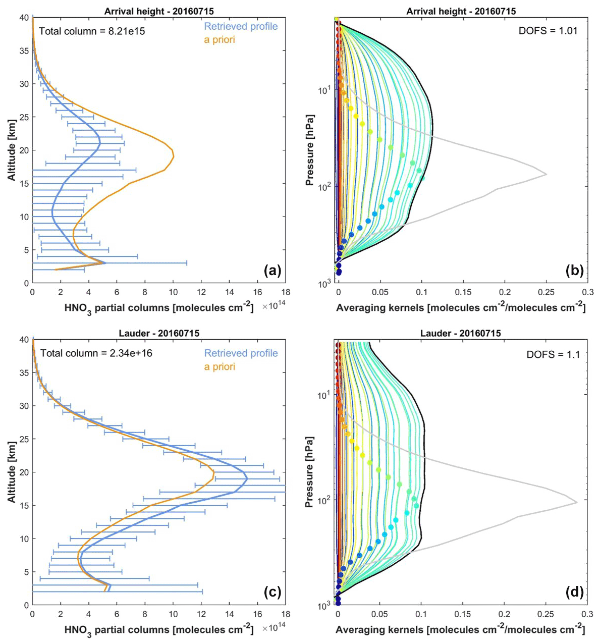
Figure 1Examples of IASI HNO3 vertical profiles (in ) with corresponding averaging kernels (in ; colored lines, with the altitude of each kernel represented by the colored dots) along with the total column averaging kernels (black) and the sensitivity profiles (grey) (both divided by 10) above Arrival Heights (77.49∘ S, 166.39∘ E, a, b) and Lauder (45.03∘ S, 169.40∘ E; c, d). The error bars associated with the HNO3 vertical profile represent the total retrieval error. The a priori profile is also represented. The total column and the DOFS values are indicated.

Figure 2Time series of daily IASI total HNO3 column (blue) co-located with MLS and of MLS total HNO3 columns (orange) within 2.5∘ × 2.5∘ grid boxes, averaged in the 70–90∘ S (a) and the 50–70∘ S (b) equivalent latitude bands. Note that the MLS total column estimates were obtained by extending the MLS partial stratospheric column values using the FORLI-HNO3 a priori information (see text for details). The error bars (blue) represent 3σ, where σ is the standard deviation around the IASI HNO3 daily average.
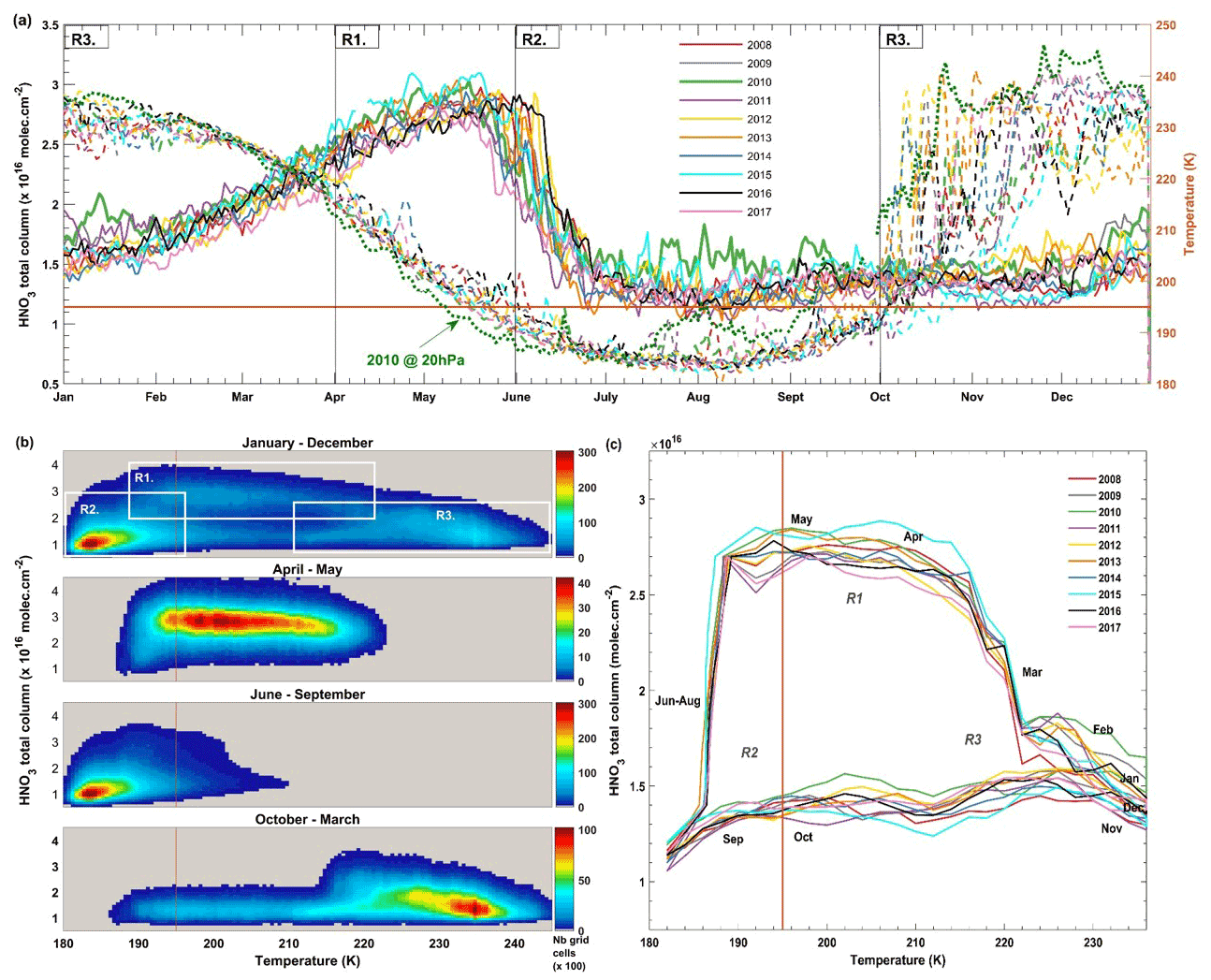
Figure 3(a) Time series of daily averaged HNO3 total columns (solid lines) and temperatures taken at 50 hPa (dashed lines) in the 70–90∘ S equivalent latitude band for the years 2008–2017. The dotted green line represents the temperatures at 20 hPa for the year 2010. (b) HNO3 total columns vs. temperature (at 50 hPa) histogram during the year 2011, over the whole year (a) and for the three defined regimes (R1–R3) separated in (a). The colors refer to the number of gridded measurements in each cell. (c) Evolution of daily averaged HNO3 total columns with the highest occurrence (in bins of 0.1 × 10¹⁶ and 2 K) as a function of the 50 hPa temperature for the years 2008–2017. The horizontal or vertical orange lines represent the 195 K threshold temperature.
The HNO3 vertical profiles are retrieved on a uniform vertical 1 km grid of 41 layers (from the surface to 40 km with an extra layer above to 60 km) in near real time by the Fast Optimal Retrieval on Layers for IASI (FORLI) software, using the optimal estimation method (Rodgers, 2000). Detailed information on the FORLI algorithm and retrieval parameters specific to HNO3 can be found in previous papers (Hurtmans et al., 2012; Ronsmans et al., 2016). For this study, only the total columns (v20151001) are used, considering (i) the low vertical resolution of IASI with only one independent piece of information (full width at half maximum – FWHM – of the averaging kernels of ∼ 30 km), (ii) the limited sensitivity of IASI to tropospheric HNO3, (iii) the dominant contribution of the stratosphere to the HNO3 total column and (iv) the largest sensitivity of IASI in the region of interest, i.e., in the low stratosphere and mid-stratosphere (from ∼ 70 to ∼ 30 hPa), where the HNO3 abundance is the highest (Ronsmans et al., 2016). The IASI measurements capture the expected depletion of HNO3 within the polar night, as illustrated in Fig. 1 with examples of vertical HNO3 profiles retrieved within the dark Antarctic vortex (above Arrival Heights) and outside the vortex (above Lauder). The retrieved profiles are shown along with their associated total retrieval error and averaging kernels (the total column averaging kernel and the so-called “sensitivity profile” are also represented; see Ronsmans et al., 2016, for more details). The total column averaging kernel (in black) indicates the sensitivity of the total column measurement to changes in the vertical distribution of HNO3; hence, the altitude to which the retrieved total column is mainly sensitive and representative, while the sensitivity profile indicates the extent to which the retrieval at one specific altitude comes from the spectral measurement rather than the a priori values. Above Arrival Heights during the dark Antarctic winter, we clearly see depleted HNO3 levels in the low stratosphere and mid-stratosphere, and the altitude of maximum sensitivity is at around 30 hPa for this case (values of ∼ 1 along the total column averaging kernel around that level). In contrast, at Lauder HNO3 levels larger than the a priori are observed in the stratosphere with a larger range of maximum sensitivity. The total columns are associated with a total retrieval error ranging from around 3 % at mid-latitudes and polar latitudes (except above Antarctica) to 25 % above cold Antarctic surface during winter, with a low absolute bias smaller than 12 % when compared to ground-based Fourier transform infrared (FTIR) measurements in polar regions over the altitude range where the IASI sensitivity is the largest (see Hurtmans et al., 2012, and Ronsmans et al., 2016, for more details). The highest retrieval error measured over the Antarctic arises from a weaker sensitivity above very cold surface with a degrees of freedom for signal (DOFS) of 0.95, as well as from a poor knowledge of the seasonally dependent and wavenumber-dependent emissivity above ice surfaces. In order to expand on the comparisons against FTIR measurements, which cannot be made during the polar night, Fig. 2a presents the time series of daily IASI total HNO3 columns co-located with MLS measurements within 2.5∘ × 2.5∘ grid boxes, averaged in the 70–90∘ S equivalent latitude band. In order to account for the vertical sensitivity of IASI, the averaging kernels associated with each co-located IASI-retrieved profile were applied to the MLS profiles for this cross-comparison. The MLS mixing ratio profiles over the 215–1.5 hPa pressure range were first interpolated to the FORLI pressure grids and extended down to the surface by using the FORLI-HNO3 a priori profile and then converted into partial columns. Similar variations in the HNO3 column are captured by the two instruments, with an particularly excellent agreement for the timing of the strong HNO3 depletion within the inner vortex core. Note that a similar good agreement between the two satellite datasets is obtained in other latitude bands (see Fig. 2b for the 50–70∘ S equivalent latitude band; the other bands are not shown).
Quality flags similar to those developed for O3 in previous IASI studies (Wespes et al., 2017) were applied a posteriori to exclude data (i) with a corresponding poor spectral fit (e.g., based on quality flags rejecting biased or sloped residuals, fits with maximum number of iterations exceeded), (ii) with less reliability (e.g., based on quality flags rejecting suspect averaging kernels, data with less sensitivity characterized by a DOFS lower than 0.9) or (iii) with tropospheric cloud contamination (defined by a fractional cloud cover ≥ 25 %). Note that the HNO3 total column distributions illustrated below use the median as a statistical average since it is more robust against the outliers than the mean.
Temperature and potential vorticity (PV) fields are taken from the ECMWF ERA-Interim Reanalysis dataset at 50 hPa and at the potential temperature of 530 K (corresponding to ∼ 20 km altitude where the IASI sensitivity to HNO3 is the highest during the Southern Hemisphere (SH) winter; Ronsmans et al., 2016), respectively. Because the HNO3 uptake by PSCs starts within a few degrees below TNAT (∼ 195.7 K at 50 hPa; Hanson and Mauersberger, 1988) depending on the meteorological conditions (Pitts et al., 2013, 2018; Hoyle et al., 2013; Lambert et al., 2016), a threshold temperature of 195 K is considered below to identify regions of potential PSC existence. The potential vorticity is used to delimit dynamically consistent areas in the polar regions. In what follows, we use either the equivalent latitudes (“eqlat”, calculated from PV fields at 530 K) or the PV values to characterize the relationship between HNO3 and temperatures in the cold polar regions. Uncertainties in ERA-Interim temperatures will also be discussed below.
Figure 3a shows the yearly HNO3 cycle (solid lines, left axis) in the southernmost equivalent latitudes (70–90∘ S) as measured by IASI over the whole study period (2008–2017). The total HNO3 variability in such equivalent latitudes has already been discussed in a previous IASI study (Ronsmans et al., 2018), where the contribution of the PSCs to the HNO3 variations was highlighted. The temperature time series, taken at 50 hPa, is represented as well (dashed lines, right axis). From Fig. 3, different regimes of HNO3 total columns vs. temperature can be observed throughout the year and from any given year to another. In particular, we define three main regimes here (R1, R2 and R3) during the HNO3 and temperature annual cycle. The full cycle and the main regimes in the 70–90∘ S eqlat region are further represented in Fig. 3b, which shows a histogram of the HNO3 total columns as a function of temperature for the year 2011. Similar histograms are observed for the other years in the 10-year study period (not shown). The horizontal and vertical orange lines in Fig. 3a and b, respectively, represent the 195 K threshold temperature used to identify the onset of HNO3 uptake by PSCs (see Sect. 2). The three regimes identified are described below.
R1 is defined by the maxima in the total HNO3 abundances covering the months of April and May (∼ 3 × 10¹⁶ ), when the 50 hPa temperature strongly decreases (from ∼ 220 to ∼ 195 K). These high HNO3 levels result from low sunlight, preventing photodissociation, and the heterogeneous hydrolysis of N2O5 to HNO3 during autumn before the formation of polar stratospheric clouds (Keys et al., 1993; Santee et al., 1999; Urban et al., 2009; de Zafra and Smyshlyaev, 2001). This period also corresponds to the onset of the development of the southern polar vortex, which is characterized by strong diabatic descent with weak latitudinal mixing across its boundary, isolating polar HNO3-rich air from lower-latitude air masses. The end of the R1 period marks the start of the strong total HNO3 decrease that intensifies later in R2.
R2, which extends from June to October, follows the onset of the strong decrease in HNO3 total columns that starts around mid-May in most years when the temperatures fall below 195 K. After a steep initial decline in total HNO3, R2 is characterized by a plateau of total HNO3 minima. For much of this regime, average HNO3 total columns are below 2 × 10¹⁶ and the 50 hPa temperatures range mostly between 180 and 190 K.
R3 starts in October when sunlight returns and the 50 hPa temperatures rise above 195 K. Despite 50 hPa temperatures increasing up to 240 K in summer, the HNO3 total columns stagnate at the R2 plateau levels (around 1.5 × 10¹⁶ ). This regime likely reflects the photolysis of NO3 and HNO3 itself (Ronsmans et al., 2018), as well as the permanent denitrification of the mid-stratosphere, caused by sedimentation of PSCs. The likely re-nitrification of the lowermost stratosphere (e.g., Braun et al., 2019; Lambert et al., 2012), where the HNO3 concentrations and the IASI sensitivity to HNO3 are lower (Ronsmans et al., 2016), cannot be inferred from the IASI total column measurements. The plateau approximately lasts until February, when HNO3 total column slowly starts increasing, reaching the April–May maximum in R1.
As illustrated in Fig. 3a, the three regimes are observed each year, albeit with some interannual variations. For instance, the sudden stratospheric warming (SSW) that occurred in 2010 (see the temperature time series at 20 hPa for the year 2010; dotted green line) yielded higher HNO3 total columns (see the solid green line in July–September) (de Laat and van Weele, 2011; Klekociuk et al., 2011; WMO, 2014; Ronsmans et al., 2018).
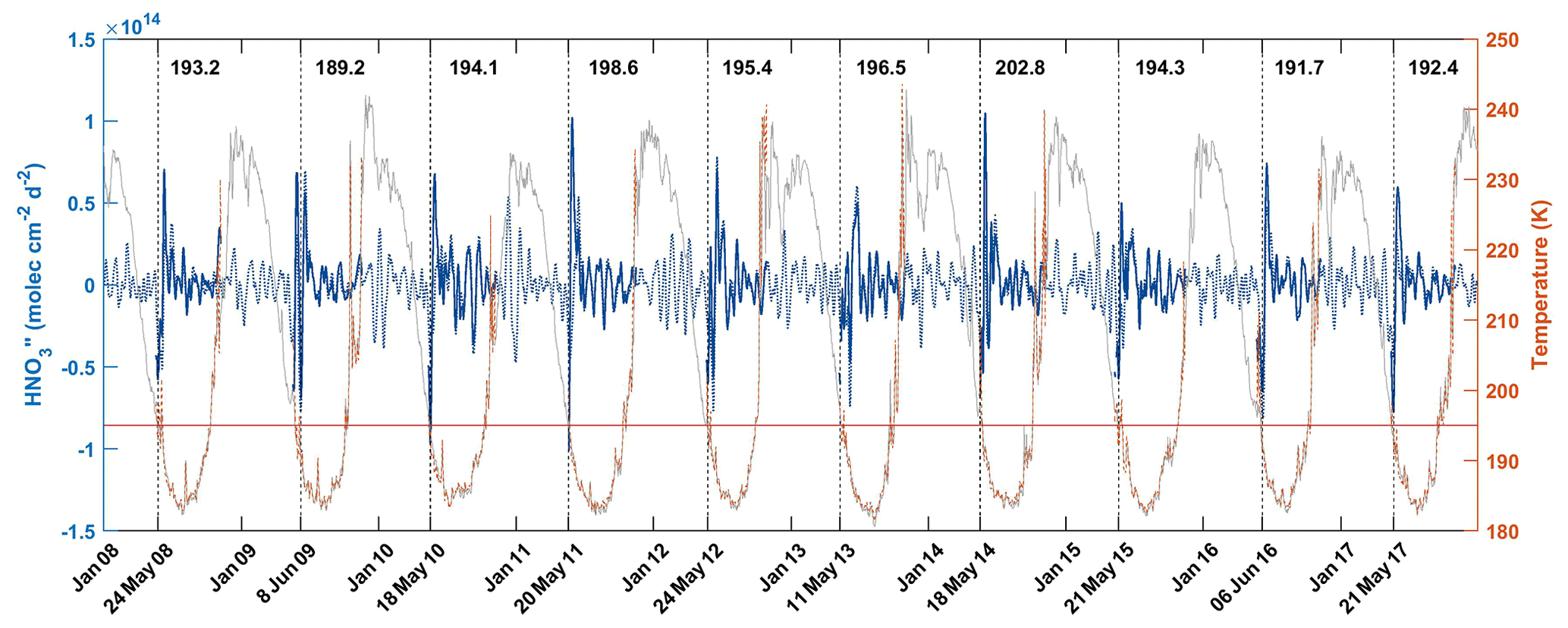
Figure 4Time series of total HNO3 second derivative (blue, left y axis) and the 50 hPa temperature (red, right y axis) in the region of potential vorticity at 530 K lower than −10 × 10−5 . The horizontal red line corresponds to the 195 K temperature. The vertical dashed lines indicate the second derivative minimum in HNO3 for each year. The corresponding dates (in bold, on the x axis) and temperatures are also indicated. The time series of total HNO3 second derivative (dashed blue) and of temperature (grey) in the 70–90∘ S eqlat band are also represented.
Figure 3c shows the evolution of the relationship between the daily averaged HNO3 (calculated from a 7 d moving average) with the highest occurrence (in bins of 0.1 × 10¹⁶ and of 2 K) and the 50 hPa temperature over the 10-year study period. The vertical orange line represents the 195 K threshold temperature. Figure 3c also highlights the large interannual variability in total HNO3 in R3, while the strong depletion in HNO3 in R2 is consistent every year. Given that PSC formation spans a large range of altitudes (typically between 10 and 30 km) (Höpfner et al., 2006, 2009; Spang et al., 2018; Pitts et al., 2018) and that IASI has maximum sensitivity to HNO3 around 50 hPa (Hurtmans et al., 2012; Ronsmans et al., 2016), the temperatures at two other pressure levels, namely 70 and 30 hPa (i.e., ∼ 15 and ∼ 25 km), have also been tested to investigate the relationship between HNO3 and temperature in the low stratosphere and mid-stratosphere. The results (not shown here) exhibit a similar HNO3 temperature behavior at the different levels with (as expected) lower and higher temperatures in R2, respectively, at 30 and at 70 hPa (temperatures down to ∼ 180 K at 30 hPa and down to ∼ 185 K at 70 hPa, as compared to temperatures down to ∼ 182 K at 50 hPa, are observed), but these values are still below the NAT formation threshold at these pressure levels (TNAT ∼ 193 K at 30 hPa and ∼ 197 K at 70 hPa) (Lambert et al., 2016). Therefore, the altitude range of maximum IASI sensitivity to HNO3 (see Sect. 2) is characterized by temperatures that are below the NAT formation threshold at these pressure levels, enabling PSC formation and the denitrification process. Furthermore, the consistency between the 195 K threshold temperature taken at 50 hPa and the onset of the strong total HNO3 depletion seen in IASI data (see Fig. 3a) is in agreement with the largest NAT area that starts to develop in June around 20 km (Spang et al., 2018), which justifies the use of the 195 K temperature at that single representative level in this study.
To identify the spatial and temporal variability of the onset of the depletion phase, the daily time evolution of HNO3 during the first 10 years of IASI measurements and the temperatures at 50 hPa are explored. In particular, the second derivative of HNO3 total column with respect to time is calculated to detect the strongest rate of decrease seen in the HNO3 time series and to identify its associated day and 50 hPa temperature.
4.1 HNO3 vs. temperature time series
Figure 4 shows the time series of the second derivative of HNO3 total column (blue) and of the temperature (red) with respect to time, averaged in the area of potential vorticity smaller than −10 × 10−5 at the potential temperature of 530 K to encompass the region inside the inner polar vortex where the temperatures are the coldest and the largest depletion of total HNO3 occurs (Ronsmans et al., 2018). The use of that PV threshold value explains the gaps in the time series during the summer when the PV does not reach such low levels, while the time series averaged in the 70–90∘ S eqlat band (dashed blue for the second derivative of HNO3 and grey for the temperature) covers the full year. Note that the HNO3 time series has been smoothed with a simple spline data interpolation function to avoid gaps in order to calculate the second derivative of HNO3 total column with respect to time as the daily second difference in HNO3 total columns. The horizontal red line shows the 195 K threshold.
As already illustrated in Fig. 3a and c, the strongest rate of HNO3 depletion (i.e., the second derivative minimum) is found closely around the time that temperatures drop below the 195 K threshold (except for the year 2009 that shows a longest delay), within a few days to a few weeks (4 to 23 d) after total HNO3 reaches its maximum, i.e., between 11 May 2013 and 8 June 2009. The 50 hPa drop temperatures, i.e., the temperature associated with the strongest rate of HNO3 depletion detected from IASI, are between 189.2 K and 198.6 K, with the exception of the year 2014, which shows a drop temperature of 202.8 K. On average over the 10 years of studied IASI measurements, a 50 hPa drop temperature of 194.2 K ± 3.8 K (1σ standard deviation) is found. Knowing that TNAT can be higher or lower depending on the atmospheric conditions and that NAT starts to nucleate from ∼ 2–4 K below TNAT (Pitts et al., 2011; Hoyle et al., 2013; Lambert et al., 2016), the results here tend to demonstrate the consistency between the 50 hPa drop temperature and the PSC existence temperature in that altitude region. Note that the range observed in the 50 hPa drop temperature could reflect variations in the preponderance of one type of PSCs over another from any given year to the next. The results further justify the use of the single 50 hPa level for characterizing and investigating the onset of HNO3 depletion from IASI. Nevertheless, given the range of maximum IASI sensitivity to HNO3 around 50 hPa, typically between 70 and 30 hPa (Ronsmans et al., 2016), the drop temperatures are also calculated at these two other pressure levels (not shown here) in order to estimate the uncertainty of the calculated drop temperature defined in this study at 50 hPa. The 30 hPa and 70 hPa drop temperatures range, respectively, over 185.7–194.9 K and over 194.8–203.7 K, with an average of 192.0 ± 2.9 and 198.0 ± 3.2 K (1σ standard deviation) over the 10 years of IASI. The average values at 30 hPa and 70 hPa fall within the 1σ standard deviation associated with the average drop temperature at 50 hPa. It is also worth noting the agreement between the drop temperatures and the NAT formation threshold at these two pressure levels (TNAT ∼ 193 K at 30 hPa and ∼ 197 K at 70 hPa) (Lambert et al., 2016). Finally, it should be noted that because the size, shape and location of the vortex vary slightly over the altitude range to which IASI is sensitive (from ∼ 30 to ∼ 70 hPa during the polar night), the use of a single potential temperature surface for the calculation of drop temperatures could introduce some uncertainties into the results. However, several tests suggest that these variations of the vortex are minor overall, and hence they have only limited influence on the identification of the inner polar vortex (delimited by a PV value of −10 × 10−5 at 530 K) and on the determination of the average drop temperature inside that region.
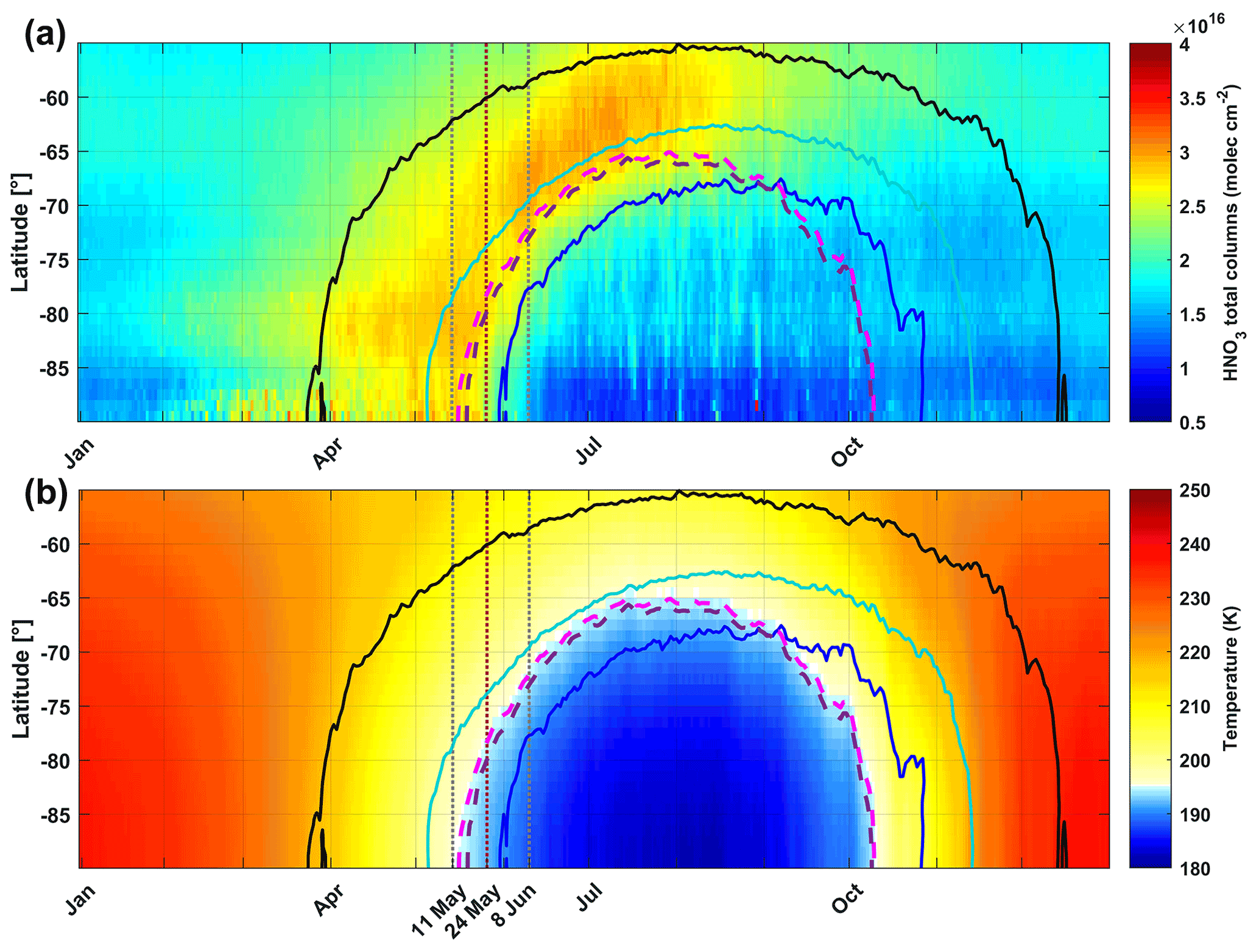
Figure 5Zonal distributions of (a) HNO3 total columns (in ) from IASI and (b) temperatures at 50 hPa from ERA-Interim (in K) in the 55–90∘ S geographical latitude band and averaged over the years 2008–2017. Three isocontours for the climatological (2008–2017) and zonally averaged PV of −5 (black), −8 (cyan) and −10 (blue) (× 10−5 ) at 530 K. The isocontours for the 195 K climatological (2008–2017) zonally averaged temperature (pink) and the averaged 194.2 K drop temperature (purple) at 50 hPa are superimposed. The vertical dashed grey lines mark the earliest and latest dates for the averaged drop temperature in the 10-year IASI record, and the red line indicates the average date for the drop temperatures calculated in the area delimited by the −10 × 10−5 PV contour.

Figure 6Zonally averaged distributions of (a) HNO3 total columns (in ) from IASI and (b) temperatures at 50 hPa from ERA-Interim (in K). The geographical latitude range is from 55–90∘ S and the isocontours are PVs of −5 (black), −8 (cyan) and −10 (blue) (× 10−5 at 530 K). The vertical dashed red lines correspond to the second derivative minima each year in the area delimited by a −10 × 10−5 PV contour.
Figure 5a and b show the climatological zonal distribution of HNO3 total columns and of the temperature at 50 hPa, respectively, spanning the 55–90∘ S geographic latitude band over the first 10 years of IASI, with three superimposed isocontour levels of potential vorticity (−10, −8 and −5 × 10⁻⁵ in blue, cyan and black, respectively), the isocontours for the 195 K temperature (pink) and the averaged 194.2 K drop temperature (purple) at 50 hPa. They further illustrate the relationship between the IASI total HNO3 columns and the 50 hPa temperatures. The climatological (2008–2017) PV isocontour of −10 × 10−5 is clearly shown to separate the region of strong depletion in total HNO3 well, according to the latitude and the time, until October. The vertical dashed red line indicates the average of the dates on which the 50 hPa drop temperatures are calculated in the area of PV ≤ −10 × 10−5 (194.2 ± 3.8 K; see Fig. 4) over the first 10 years of IASI. It shows that the strongest rate of HNO3 depletion occurs on average at the end of May (24 May), a few days after the temperature decreases below 195 K. The yearly zonally averaged time series over the 10-year study period can be found in Fig. 6, which shows that IASI measures similar HNO3 total column zonal distributions every year, particularly with respect to the edge of the collar region and the region of strong depletion (respectively delimited by the PV isocontours of −5 × 10⁻⁵ and −10 × 10−5 at 530 K). Like for Fig.4, the exact timing of the few days between the time that temperatures drop below the 195 K threshold and the start of the HNO3 depletion is visible every year in Fig. 6. A longest delay is also observed for the year 2009. Note that the mismatch between the 10-year average of the dates on which the 195 K threshold temperature is reached and that of the dates for the drop temperatures (see Fig. 5a and b) is driven by the year 2013, which is characterized by the lowest temperatures during the Antarctic winter over the 10-year study period and hence the earliest date for the drop temperature (11th of May; see Figs. 4 and 6).
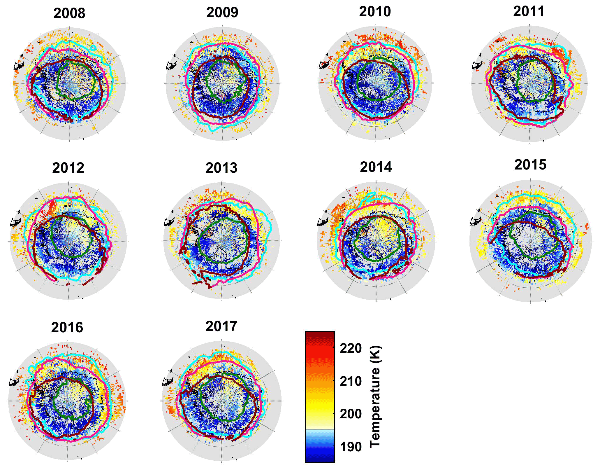
Figure 7Spatial distribution (1∘ × 1∘) of the drop temperature at 50 hPa (K) (calculated from the total HNO3 second derivative minima) for each year of IASI (2008–2017) in a region defined by a PV of −8 × 10⁻⁵ . The isocontours of −10 × 10−5 at 530 K for the averaged PV (in green) and the minimum PV (in cyan) encountered over the period 10 May–15 July for each year and the isocontours of 195 K at 50 hPa for the averaged (in red) and minimum (in pink) temperatures over the same period are represented.
4.2 Spatial distribution of drop temperatures
To explore the capability of IASI to monitor the onset of HNO3 depletion at a large scale, Fig. 7 shows, for each year of the study period, the spatial distribution of the 50 hPa drop temperatures based on the second derivative minima of total HNO3 averaged in 1∘ × 1∘ grid cells. The region of interest here is delimited by a PV value of −8 × 10⁻⁵ at 530 K in order to investigate an area a bit larger than the inner vortex core that was the focus of the preceding discussion (delineated in green in Fig. 7 by the PV isocontour of −10 × 10−5 averaged over the interval 10 May to 15 July). The isocontour of −10 × 10−5 for the minimum PV (in cyan) encountered at 530 K over the 10 May to 15 July period for each year, as well as the isocontours of 195 K for the average temperatures and the minimum temperatures, are also represented. The calculated drop temperatures corresponding to the onset of HNO3 depletion inside the averaged PV isocontour are found to vary between ∼ 180 and ∼ 210 K, and the corresponding dates range between ∼ mid-May and mid-July (not shown here). Although the range of drop temperatures and dates for 1∘ × 1∘ bins is broader than that found for the inner vortex averages discussed above, the results are qualitatively consistent. For example, the year 2014, which shows the highest inner vortex average drop temperature in Fig. 4, is characterized by the highest drop temperatures above the eastern Antarctic. Note, however, that the high extremes in the drop temperature, mainly found above the eastern Antarctic, should be considered with caution: they correspond to specific regions above ice surfaces with emissivity features that are known to yield errors in the IASI retrievals (Hurtmans et al., 2012; Ronsmans et al., 2016). Indeed, bright land surfaces such as ice might in some cases lead to poor HNO3 retrievals. Although wavenumber-dependent surface emissivity atlases are used in FORLI (Hurtmans et al., 2012), this parameter remains critical and causes poorer retrievals that in some instances pass through the series of quality filters and could affect the drop temperature calculation.
The averaged isocontour of 195 K encircles the area of HNO3 drop temperatures lower than 195 K (typically from ∼ 187 to ∼ 195 K) fairly well, which means that the bins inside that area include air masses that experience the NAT threshold temperature for a long time over the 10 May–15 July period. That area encompasses the inner vortex core (delimited by the isocontour of −10 × 10−5 for the PV averaged over the 10 May–15 July period) and shows pronounced minima (lower than −0.5 × 10¹⁴ ) in the second derivative of the HNO3 total column with respect to time (not shown here), which both indicate a strong and rapid HNO3 depletion. The area enclosed between the two isocontours of 195 K for the temperatures, the averaged one and the one for the minimum temperatures, shows generally higher drop temperatures and the weakest minima (larger than −0.5 × 10¹⁴ ) in the second derivative of the HNO3 total column (not shown). That area is also typically enclosed by the isocontour of −10 × 10−5 for the minimum PV, meaning that the bins inside correspond, at least for a single day over the 10 May–15 July period, to air masses located at the inner edge of the vortex and characterized by temperature lower than the NAT threshold temperature. The fact that the weakest minima in the second derivative of total HNO3 are observed in that area (not shown) indicates a weak and slow HNO3 depletion that might be explained by air masses at the inner edge of the vortex experiencing only a short period with temperatures below the NAT threshold temperature. It could also reflect mixing with strongly HNO3-depleted and colder air masses from the inner vortex core. Mixing with these already depleted air masses could also explain the higher drop temperatures detected in those bins. These sometimes unrealistic high drop temperatures are generally detected later (after the strong HNO3 depletion occurs in the inner vortex core, i.e., after the 10 May–15 July period considered here – not shown), which supports the transport in those bins of previously HNO3-depleted air masses and the likely mixing at the edge of the vortex. Note, however, that previous studies have shown a generally weak mixing in the Antarctic between the edge region and the vortex core (e.g., Roscoe et al., 2012). Finally, these spatial variations might also partly reflect some uncertainty in the drop temperature calculation, introduced by the use of temperature at a single pressure level (50 hPa) and PV on a single potential temperature surface (530 K) while the sensitivity of IASI to changes in the HNO3 profiles extends over a range from ∼ 30 to ∼ 70 hPa during the polar night. It should be noted that biases in the ECMWF ERA-Interim temperatures used in this work are too small to explain the large range of drop temperatures calculated here. Indeed, Lambert and Santee (2018) found only a small warm bias, with median differences around 0.5 K, reaching 0–0.25 K in the southernmost regions of the globe at ∼ 68–21 hPa where PSCs form, through comparisons with the Constellation Observing System for Meteorology, Ionosphere and Climate (COSMIC) data.
Except above some parts of Antarctica that are prone to larger retrieval errors and where unrealistic high drop temperatures are found, the overall range in the 50 hPa drop temperature for total HNO3 inside the isocontour for the averaged temperature of 195 K typically extends from ∼ 187 to ∼ 195 K, which falls within the range of PSC nucleation temperature at 50 hPa: from slightly below TNAT to around 3–4 K below the ice frost point – Tice – depending on atmospheric conditions, the TTE and the specific formation mechanism (i.e., the type of PSC developing) (Pitts et al., 2011; Peter and Grooß, 2012; Hoyle et al., 2013). This underlines the benefit of the excellent spatial and temporal coverage of IASI well, as it allows for the rapid and critical depletion phase to be captured in detail over a large scale.
In this paper, we have explored the added value of the dense HNO3 total column dataset provided by the IASI/MetOp-A satellite over a full decade (2008–2017) for monitoring the stratospheric depletion phase that occurs each year in the SH and for investigating its relationship to the NAT formation temperature. To that end, we focused on and delimited the coldest polar region of the SH using a specific PV value at 530 K (∼ 50 hPa, PV of −10 × 10−5 ) and stratospheric temperatures at 50 hPa taken from the ECMWF ERA-Interim reanalysis. That single representative pressure level has been considered in this study given the maximum sensitivity of IASI to HNO3 around that level, which lies in the range where the PSCs formation and denitrification processes occur.
The annual cycle of total HNO3, as observed from IASI, has first been characterized according to the temperature evolution. Three regimes (R1 to R3) in the total HNO3–50 hPa temperature relationship were highlighted from the time series over the SH polar region: R1 is defined during April and May and characterized by a rapid decrease in 50 hPa temperatures while HNO3 accumulates over the pole; R2, from June to October, follows the onset of the depletion that starts around mid-May in most years when the 50 hPa temperatures fall below 195 K (considered here as the onset of PSC nucleation phase at that level), with a strong consistency from year to year; R3, defined from October through March when total HNO3 remains at low R2 plateau levels despite the return of sunlight and heat, characterizes the strong denitrification of the stratosphere, likely due to PSC sedimentation to lower levels where the IASI sensitivity is low. For each year over the 10-year study period, the use of the second derivative of the HNO3 column vs. time was then found to be particularly valuable to detect the onset of the HNO3 condensation into PSCs. On average, it is captured from IASI a few days before June with a delay of 4–23 d after the maximum in total HNO3. The corresponding temperatures (“drop temperatures”) were detected between 189.2 and 202.8 K (194.2 ± 3.8 K on average over the 10 years), which tends to demonstrate the good consistency between the 50 hPa drop temperature and the PSC formation temperatures in that altitude region. Finally, the annual and spatial variability (within 1∘ × 1∘) in the drop temperature was further explored from IASI total HNO3. Inside the isocontours of 195 K for the average temperatures and of −10 × 10−5 for the averaged PV at 530 K, the drop temperatures are detected between around mid-May and mid-July, typically range between ∼ 187 to ∼ 195 K, and are associated with the lowest minima (lower than −0.5 × 10¹⁴ ) in the second derivative of the HNO3 total column with respect to time, indicating a strong and rapid HNO3 depletion. Except for unrealistic drop temperatures (∼ 210 K) that were found in some years above eastern Antarctica and suspected to result from unfiltered poor-quality retrievals arising from emissivity issues above ice, the range of drop temperatures is interestingly found to be in line with the PSC nucleation temperature that is known from previous studies to strongly depend on several factors (e.g., meteorological conditions, HNO3 vapor pressure, temperature threshold exposure, presence of meteoritic dust). At the edge of the vortex, considering the isocontours of 195 K for the minimum temperatures or of −10 × 10−5 for the minimum PV, higher and later drop temperatures, and the weakest minima in the second derivative of the HNO3 total column with respect to time, indicating a slow HNO3 depletion, are found. These likely result from a short temperature threshold exposure or mixing with already depleted air masses from the inner vortex core. The results of this study highlight the ability of IASI to measure the variations in total HNO3 and to specifically capture and monitor the rapid depletion phase over the whole Antarctic region.
We show in this study that the IASI dataset allows the variability of stratospheric HNO3 throughout the year (including the polar night) in the Antarctic to be captured. In that respect, it offers observational means to monitor the relation of HNO3 to temperature and the related formation of PSCs. Despite the limited vertical resolution of IASI, which does not allow investigation of the HNO3 uptake by the different types of PSCs during their formation and growth along the vertical profile, the HNO3 total column measurements from IASI constitute an important new dataset for exploring the strong polar depletion over the whole stratosphere. This is particularly relevant considering the mission continuity, which will span several decades with the planned follow-on missions. Indeed, thanks to the three successive instruments (IASI-A launched in 2006 and is still operating, IASI-B launched in 2012, and IASI-C launched in 2018) that demonstrate the excellent stability of the level 1 radiances, the measurements will soon provide an unprecedented long-term dataset of HNO3 total columns. Further work could also make use of this unique dataset to investigate the relation between HNO3, O3 and meteorology in the changing climate.
The IASI HNO3 data processed with FORLI-HNO3 v0151001 are available upon request to the corresponding author.
GR and CW performed the analysis, wrote the manuscript and prepared the figures. LC contributed to the analysis. SS, PFC and LC contributed to the interpretation of the results. DH was responsible for the retrieval algorithm development and the processing of the IASI HNO3 dataset. All authors contributed to the writing of the text and reviewed the manuscript.
The contact author has declared that none of the authors has any competing interests.
Publisher's note: Copernicus Publications remains neutral with regard to jurisdictional claims in published maps and institutional affiliations.
IASI has been developed and built under the responsibility of the Centre National d'Etudes Spatiales (CNES, France). It is flown on board the MetOp satellites as part of the EUMETSAT Polar System. The IASI L1 data are received through the EUMETCast near-real-time data distribution service. We also would like to thank the three reviewers for their helpful comments and corrections and, in particular, Michelle L. Santee for her in-depth reviews, which have substantially improved the paper quality.
The research was funded by the F.R.S.-FNRS, the Belgian State Federal Office for Scientific, Technical and Cultural Affairs (Prodex arrangement 4000111403 IASI.FLOW), and EUMETSAT through the Satellite Application Facility on Atmospheric Composition Monitoring (ACSAF). Gaetane Ronsmans is grateful to the Fonds pour la Formation à la Recherche dans l'Industrie et dans l'Agriculture of Belgium for a PhD grant (Boursier FRIA). Lieven Clarisse is a research associate supported by the F.R.S.-FNRS. Cathy Clerbaux is grateful to the Centre National d'Etudes Spatiales (CNES) for financial support. Susan Solomon is supported by the National Science Foundation (grant no. NSF-1539972).
This paper was edited by Michael Pitts and reviewed by Michelle Santee and three anonymous referees.
Braun, M., Grooß, J.-U., Woiwode, W., Johansson, S., Höpfner, M., Friedl-Vallon, F., Oelhaf, H., Preusse, P., Ungermann, J., Sinnhuber, B.-M., Ziereis, H., and Braesicke, P.: Nitrification of the lowermost stratosphere during the exceptionally cold Arctic winter 2015–2016, Atmos. Chem. Phys., 19, 13681–13699, https://doi.org/10.5194/acp-19-13681-2019, 2019.
Carslaw, K. S., Luo, B. P., and Peter, T.: An analytical expression for the composition of aqueous {HNO3-H2SO4-H2O} stratospheric aerosols including gas phase removal of HNO3, Geophys. Res. Lett., 22, 1877–1880, https://doi.org/10.1029/95GL01668, 1995.
Carslaw, K. S., Wirth, M., Tsias, A., Luo, B. P., Dörnbrack, A., Leutbecher, M., Volkert, H., Renger, W., Bacmeister, J. T., Reimer, E., and Peter, T.: Increased stratospheric ozone depletion due to mountain-induced atmospheric waves, Nature, 391, 675–678, https://doi.org/10.1038/35589, 1998.
Clerbaux, C., Boynard, A., Clarisse, L., George, M., Hadji-Lazaro, J., Herbin, H., Hurtmans, D., Pommier, M., Razavi, A., Turquety, S., Wespes, C., and Coheur, P.-F.: Monitoring of atmospheric composition using the thermal infrared IASI/MetOp sounder, Atmos. Chem. Phys., 9, 6041–6054, https://doi.org/10.5194/acp-9-6041-2009, 2009.
de Laat, A. T. J. and van Weele, M.: The 2010 Antarctic ozone hole: Observed reduction in ozone destruction by minor sudden stratospheric warmings, Scientific Reports, 1, 38, https://doi.org/10.1038/srep00038, 2011.
de Zafra, R. and Smyshlyaev, S. P.: On the formation of HNO3 in the Antarctic mid to upper stratosphere in winter, J. Geophys. Res., 116, 23115–23125, https://doi.org/10.1029/2000JD000314, 2001.
Grooß, J.-U., Engel, I., Borrmann, S., Frey, W., Günther, G., Hoyle, C. R., Kivi, R., Luo, B. P., Molleker, S., Peter, T., Pitts, M. C., Schlager, H., Stiller, G., Vömel, H., Walker, K. A., and Müller, R.: Nitric acid trihydrate nucleation and denitrification in the Arctic stratosphere, Atmos. Chem. Phys., 14, 1055–1073, https://doi.org/10.5194/acp-14-1055-2014, 2014.
Hanson, D. and Mauersberger, K.: Laboratory studies of the nitric acid trihydrate: Implications for the south polar stratosphere, Geophys. Res. Lett., 15, 855–858, https://doi.org/10.1029/GL015i008p00855, 1988.
Harris, N. R. P., Lehmann, R., Rex, M., and von der Gathen, P.: A closer look at Arctic ozone loss and polar stratospheric clouds, Atmos. Chem. Phys., 10, 8499–8510, https://doi.org/10.5194/acp-10-8499-2010, 2010.
Hilton, F., Armante, R., August, T., Barnet, C., Bouchard, A., Camy-Peyret, C., Capelle, V., Clarisse, L., Clerbaux, C., Coheur, P.-F., Collard, A., Crevoisier, C., Dufour, G., Edwards, D., Faijan, F., Fourrié, N., Gambacorta, A., Goldberg, M., Guidard, V., Hurtmans, D., Illingworth, S., Jacquinet-Husson, N., Kerzenmacher, T., Klaes, D., Lavanant, L., Masiello, G., Matricardi, M., McNally, A., Newman, S., Pavelin, E., Payan, S., Péquignot, E., Peyridieu, S., Phulpin, T., Remedios, J., Schlüssel, P., Serio, C., Strow, L., Stubenrauch, C., Taylor, J., Tobin, D., Wolf, W., and Zhou, D.: Hyperspectral Earth Observation from IASI: Five Years of Accomplishments, B. Am. Meteorol. Soc., 93, 347–370, https://doi.org/10.1175/BAMS-D-11-00027.1, 2012.
Hoffmann, L., Spang, R., Orr, A., Alexander, M. J., Holt, L. A., and Stein, O.: A decadal satellite record of gravity wave activity in the lower stratosphere to study polar stratospheric cloud formation, Atmos. Chem. Phys., 17, 2901–2920, https://doi.org/10.5194/acp-17-2901-2017, 2017.
Höpfner, M., Luo, B. P., Massoli, P., Cairo, F., Spang, R., Snels, M., Di Donfrancesco, G., Stiller, G., von Clarmann, T., Fischer, H., and Biermann, U.: Spectroscopic evidence for NAT, STS, and ice in MIPAS infrared limb emission measurements of polar stratospheric clouds, Atmos. Chem. Phys., 6, 1201–1219, https://doi.org/10.5194/acp-6-1201-2006, 2006.
Höpfner, M., Pitts, M. C., and Poole, L. R.: Comparison between CALIPSO and MIPAS observations of polar stratospheric clouds, J. Geophys. Res.-Atmos., 114, 1–15, https://doi.org/10.1029/2009JDO12114, 2009.
Hoyle, C. R., Engel, I., Luo, B. P., Pitts, M. C., Poole, L. R., Grooß, J.-U., and Peter, T.: Heterogeneous formation of polar stratospheric clouds – Part 1: Nucleation of nitric acid trihydrate (NAT), Atmos. Chem. Phys., 13, 9577–9595, https://doi.org/10.5194/acp-13-9577-2013, 2013.
Hurtmans, D., Coheur, P.-F., Wespes, C., Clarisse, L., Scharf, O., Clerbaux, C., Hadji-Lazaro, J., George, M., and Turquety, S.: FORLI radiative transfer and retrieval code for IASI, J. Quant. Spectrosc. Ra., 113, 1391–1408, https://doi.org/10.1016/j.jqsrt.2012.02.036, 2012.
James, A. D., Brooke, J. S. A., Mangan, T. P., Whale, T. F., Plane, J. M. C., and Murray, B. J.: Nucleation of nitric acid hydrates in polar stratospheric clouds by meteoric material, Atmos. Chem. Phys., 18, 4519–4531, https://doi.org/10.5194/acp-18-4519-2018, 2018.
Keys, J. G., Johnston, P. V., Blatherwick, R. D., and Murcray, F. J.: Evidence for heterogeneous reactions in the Antarctic autumn stratosphere, Nature, 361, 49–51, https://doi.org/10.1038/361049a0, 1993.
Klekociuk, A., Tully, M., Alexander, S., Dargaville, R., Deschamps, L., Fraser, P., Gies, H., Henderson, S., Javorniczky, J., Krummel, P., Petelina, S., Shanklin, J., Siddaway, J., and Stone, K.: The Antarctic ozone hole during 2010, Aust. Meteorol. Ocean., 61, 253–267, https://doi.org/10.22499/2.6104.006, 2011.
Koop, T., Luo, B., Tsias, A., and Peter, T.: Water activity as the determinant for homogeneous ice nucleation in aqueous solutions, Nature, 406, 611–614, https://doi.org/10.1038/35020537, 2000.
Lambert, A. and Santee, M. L.: Accuracy and precision of polar lower stratospheric temperatures from reanalyses evaluated from A-Train CALIOP and MLS, COSMIC GPS RO, and the equilibrium thermodynamics of supercooled ternary solutions and ice clouds, Atmos. Chem. Phys., 18, 1945–1975, https://doi.org/10.5194/acp-18-1945-2018, 2018.
Lambert, A., Santee, M. L., Wu, D. L., and Chae, J. H.: A-train CALIOP and MLS observations of early winter Antarctic polar stratospheric clouds and nitric acid in 2008, Atmos. Chem. Phys., 12, 2899–2931, https://doi.org/10.5194/acp-12-2899-2012, 2012.
Lambert, A., Santee, M. L., and Livesey, N. J.: Interannual variations of early winter Antarctic polar stratospheric cloud formation and nitric acid observed by CALIOP and MLS, Atmos. Chem. Phys., 16, 15219–15246, https://doi.org/10.5194/acp-16-15219-2016, 2016.
Lowe, D. and MacKenzie, A. R.: Polar stratospheric cloud microphysics and chemistry, J. Atmos. So.-Terr. Phy., 70, 13–40, https://doi.org/10.1016/j.jastp.2007.09.011, 2008.
Molleker, S., Borrmann, S., Schlager, H., Luo, B., Frey, W., Klingebiel, M., Weigel, R., Ebert, M., Mitev, V., Matthey, R., Woiwode, W., Oelhaf, H., Dörnbrack, A., Stratmann, G., Grooß, J.-U., Günther, G., Vogel, B., Müller, R., Krämer, M., Meyer, J., and Cairo, F.: Microphysical properties of synoptic-scale polar stratospheric clouds: in situ measurements of unexpectedly large HNO3−containing particles in the Arctic vortex, Atmos. Chem. Phys., 14, 10785–10801, https://doi.org/10.5194/acp-14-10785-2014, 2014.
Murphy, D. M. and Koop, T.: Review of the vapour pressures of ice and supercooled water for atmospheric applications, Q. J. Roy. Meteor. Soc., 131, 1539–1565, https://doi.org/10.1256/qj.04.94, 2005.
Peter, T.: Microphysics and heterogeneous chemistry of polar stratospheric clouds, Annu. Rev. Phys. Chem., 48, 785–822, https://doi.org/10.1146/annurev.physchem.48.1.785, 1997.
Peter, T. and Grooß, J.-U.: Chapter 4. Polar Stratospheric Clouds and Sulfate Aerosol Particles: Microphysics, Denitrification and Heterogeneous Chemistry, in: Stratospheric Ozone Depletion and Climate Change, edited by: Muller, R., The Royal Society of Chemistry, Thomas Graham House, Science Park, Milton Road, Cambridge CB4 0WF, UK, https://doi.org/10.1039/9781849733182-00108, pp. 108–144, 2012.
Piccolo, C. and Dudhia, A.: Precision validation of MIPAS-Envisat products, Atmos. Chem. Phys., 7, 1915–1923, https://doi.org/10.5194/acp-7-1915-2007, 2007.
Pitts, M. C., Poole, L. R., Dörnbrack, A., and Thomason, L. W.: The 2009–2010 Arctic polar stratospheric cloud season: a CALIPSO perspective, Atmos. Chem. Phys., 11, 2161–2177, https://doi.org/10.5194/acp-11-2161-2011, 2011.
Pitts, M. C., Poole, L. R., Lambert, A., and Thomason, L. W.: An assessment of CALIOP polar stratospheric cloud composition classification, Atmos. Chem. Phys., 13, 2975–2988, https://doi.org/10.5194/acp-13-2975-2013, 2013.
Pitts, M. C., Poole, L. R., and Gonzalez, R.: Polar stratospheric cloud climatology based on CALIPSO spaceborne lidar measurements from 2006 to 2017, Atmos. Chem. Phys., 18, 10881–10913, https://doi.org/10.5194/acp-18-10881-2018, 2018.
Rodgers, C. D.: Inverse Methods for Atmospheric Sounding – Theory and Practice, vol. 2 of Series on Atmospheric Oceanic and Planetary Physics, World Scientific Publishing Co. Pte. Ltd., Oxford, https://doi.org/10.1142/9789812813718, 2000.
Roscoe, H. K., Feng, W., Chipperfield, M. P., Trainic, M., and Shuckburgh, E. F.: The existence of the edge region of the Antarctic stratospheric vortex, J. Geophys. Res., 117, D04301, https://doi.org/10.1029/2011JD015940, 2012.
Ronsmans, G., Langerock, B., Wespes, C., Hannigan, J. W., Hase, F., Kerzenmacher, T., Mahieu, E., Schneider, M., Smale, D., Hurtmans, D., De Mazière, M., Clerbaux, C., and Coheur, P.-F.: First characterization and validation of FORLI−HNO3 vertical profiles retrieved from IASI/Metop, Atmos. Meas. Tech., 9, 4783–4801, https://doi.org/10.5194/amt-9-4783-2016, 2016.
Ronsmans, G., Wespes, C., Hurtmans, D., Clerbaux, C., and Coheur, P.-F.: Spatio-temporal variations of nitric acid total columns from 9 years of IASI measurements – a driver study, Atmos. Chem. Phys., 18, 4403–4423, https://doi.org/10.5194/acp-18-4403-2018, 2018.
Santee, M. L., Manney, G. L., Froidevaux, L., Read, W. G., and Waters, J. W.: Six years of UARS Microwave Limb Sounder HNO3 observations: Seasonal, interhemispheric, and interannual variations in the lower stratosphere, J. Geophys. Res., 104, 8225–8246, https://doi.org/10.1029/1998JD100089, 1999.
Santee, M. L., Lambert, A., Read, W. G., Livesey, N. J., Cofield, R. E., Cuddy, D. T., Daffer, W. H., Drouin, B. J., Froidevaux, L., Fuller, R. A., Jarnot, R. F., Knosp, B. W., Manney, G. L., Perun, V. S., Snyder, W. V., Stek, P. C., Thurstans, R. P., Wagner, P. A., Waters, J. W., Muscari, G., de Zafra, R. L., Dibb, J. E., Fahey, D. W., Popp, P. J., Marcy, T. P., Jucks, K. W., Toon, G. C., Stachnik, R. A., Bernath, P. F., Boone, C. D., Walker, K. A., Urban, J., and Murtagh, D.: Validation of the Aura Microwave Limb Sounder HNO3 measurements, J. Geophys. Res., 112, 1–22, https://doi.org/10.1029/2007JD008721, 2007.
Schreiner, J., Voigt, C., Weisser, C., Kohlmann, A., Mauersberger, K., Deshler, T., Kröger, C., Rosen, J., Kjome, N., Larsen, N., Adriani, A., Cairo, F., Donfrancesco, G. D., Ovarlez, J., Ovarlez, H., and Dörnbrack, A.: Chemical , microphysical , and optical properties of polar stratospheric clouds, J. Geophys. Res., 108, 1–10, https://doi.org/10.1029/2001JD000825, 2003.
Sheese, P. E., Walker, K. A., Boone, C. D., Bernath, P. F., Froidevaux, L., Funke, B., Raspollini, P., and von Clarmann, T.: ACE-FTS ozone, water vapour, nitrous oxide, nitric acid, and carbon monoxide profile comparisons with MIPAS and MLS, J. Quant. Spectrosc. Ra., 186, 63–80, https://doi.org/10.1016/j.jqsrt.2016.06.026, 2017.
Snels, M., Scoccione, A., Di Liberto, L., Colao, F., Pitts, M., Poole, L., Deshler, T., Cairo, F., Cagnazzo, C., and Fierli, F.: Comparison of Antarctic polar stratospheric cloud observations by ground-based and space-borne lidar and relevance for chemistry–climate models, Atmos. Chem. Phys., 19, 955–972, https://doi.org/10.5194/acp-19-955-2019, 2019.
Solomon, S.: Stratospheric ozone depletion: A review of concepts and history, Rev. Geophys., 37, 275–316, https://doi.org/10.1029/1999RG900008, 1999.
Spang, R., Hoffmann, L., Höpfner, M., Griessbach, S., Müller, R., Pitts, M. C., Orr, A. M. W., and Riese, M.: A multi-wavelength classification method for polar stratospheric cloud types using infrared limb spectra, Atmos. Meas. Tech., 9, 3619–3639, https://doi.org/10.5194/amt-9-3619-2016, 2016.
Spang, R., Hoffmann, L., Müller, R., Grooß, J.-U., Tritscher, I., Höpfner, M., Pitts, M., Orr, A., and Riese, M.: A climatology of polar stratospheric cloud composition between 2002 and 2012 based on MIPAS/Envisat observations, Atmos. Chem. Phys., 18, 5089–5113, https://doi.org/10.5194/acp-18-5089-2018, 2018.
Toon, O. B., Hamill, P., Turco, R. P., and Pinto, J.: Condensation of HNO3 and HCl in the winter polar stratospheres, Geophys. Res. Lett., 13, 1284–1287, https://doi.org/10.1029/GL013i012p01284, 1986.
Tritscher, I., Pitts, M. C., Poole, L. R., Alexander, S. P., Cairo, F., Chipperfield, M. P., Grooß, J.-U., Höpfner, M., Lambert, A., Luo, B., Molleker, S., Orr, A., Salawitch, R., Snels, M., Spang, R., Woiwode, W., and Peter, T.: Polar stratospheric clouds: Satellite observations, processes, and role in ozone depletion, Rev. Geophys., 59, e2020RG000702, https://doi.org/10.1029/2020RG000702, 2021.
Urban, J., Pommier, M., Murtagh, D. P., Santee, M. L., and Orsolini, Y. J.: Nitric acid in the stratosphere based on Odin observations from 2001 to 2009 – Part 1: A global climatology, Atmos. Chem. Phys., 9, 7031–7044, https://doi.org/10.5194/acp-9-7031-2009, 2009.
Voigt, C., Schreiner, J., Kohlmann, A., Zink, P., Mauersberger, K., Larsen, N., Deshler, T., Kro, C., Rosen, J., Adriani, A., Cairo, F., Donfrancesco, G. D., Viterbini, M., Ovarlez, J., Ovarlez, H., and David, C.: Nitric Acid Trihydrate (NAT) in Polar Stratospheric Clouds, Science, 290, 1756–1758, https://doi.org/10.1126/science.290.5497.1756, 2000.
Voigt, C., Larsen, N., Deshler, T., Kröger, C., Schreiner, J., Mauersberger, K., Luo, B., Adriani, A., Cairo, F., Di Donfrancesco, G., Ovarlez, J.,Ovarlez, H., Dörnbrack, A., Knudsen, B., and Rosen, J.: In situ mountainwave polar stratospheric cloud measurements: Implications for nitric acid trihydrate formation, J. Geophys. Res., 108, 8331, https://doi.org/10.1029/2001JD001185, 2003.
Voigt, C., Schlager, H., Luo, B. P., Dörnbrack, A., Roiger, A., Stock, P., Curtius, J., Vössing, H., Borrmann, S., Davies, S., Konopka, P., Schiller, C., Shur, G., and Peter, T.: Nitric Acid Trihydrate (NAT) formation at low NAT supersaturation in Polar Stratospheric Clouds (PSCs), Atmos. Chem. Phys., 5, 1371–1380, https://doi.org/10.5194/acp-5-1371-2005, 2005.
von König, M.: Using gas-phase nitric acid as an indicator of PSC composition, J. Geophys. Res., 107, 8265, https://doi.org/10.1029/2001jd001041, 2002.
Wang, X. and Michelangeli, D. V.: A review of polar stratospheric cloud formation, China Part., 4, 261–271, https://doi.org/10.1016/S1672-2515(07)60275-9, 2006.
Wegner, T., Grooß, J.-U., von Hobe, M., Stroh, F., Sumińska-Ebersoldt, O., Volk, C. M., Hösen, E., Mitev, V., Shur, G., and Müller, R.: Heterogeneous chlorine activation on stratospheric aerosols and clouds in the Arctic polar vortex, Atmos. Chem. Phys., 12, 11095–11106, https://doi.org/10.5194/acp-12-11095-2012, 2012.
Wespes, C., Hurtmans, D., Clerbaux, C., and Coheur, P.-F.: O3 variability in the troposphere as observed by IASI over 2008-2016: Contribution of atmospheric chemistry and dynamics, J. Geophys. Res.-Atmos., 122, 2429–2451, https://doi.org/10.1002/2016JD025875, 2017.
WMO: Scientific Assessment of Ozone Depletion: 2014, Global Ozone Research and Monitoring Project – Report No. 55, World Meteorological Organization, Geneva, Switzerland, 2014.
Zhu, Y., Toon, O. B., Lambert, A., Kinnison, D. E., Brakebusch, M., Bardeen, C. G., Mills, M. J., and English, J. M.: Development of a Polar Stratospheric Cloud Model within the Community Earth System Model using constraints on Type I PSCs from the 2010-2011 Arctic winter, J. Adv. Model. Earth Sy., 7, 551–585, https://doi.org/10.1002/2015ms000427, 2015.
Zondlo, M. A., Hudson, P. K., Prenni, A. J., and Tolbert, M. A.: Chemistry and microphysics of polar stratospheric clouds and cirrus clouds, Annu. Rev. Phys. Chem., 51, 473–499, 2000.
drop temperature) corresponding to the onset of denitrification in Antarctic winter for each year.