the Creative Commons Attribution 4.0 License.
the Creative Commons Attribution 4.0 License.
 | 19 Aug 2022
Analysis of global trends of total column water vapour from multiple years of OMI observations
Christian Borger
Steffen Beirle
In this study, we investigate trends in total column water vapour (TCWV) retrieved from measurements of the Ozone Monitoring Instrument (OMI) for the time range between January 2005 to December 2020. The trend analysis reveals, on global average, an annual increase in the TCWV amount of approximately +0.054 kg m−2 yr−1 or +0.21 % yr−1. After the application of a Z test (to the significance level of 5 %) and a false discovery rate (FDR) test to the results of the trend analysis, mainly positive trends remain, in particular over the northern subtropics in the eastern Pacific.
Combining the relative TCWV trends with trends in air temperature, we also analyse trends in relative humidity (RH) on the local scale. This analysis reveals that the assumption of temporally invariant RH is not always fulfilled, as we obtain increasing and decreasing RH trends over large areas of the ocean and land surface and also observe that these trends are not limited to arid and humid regions, respectively. For instance, we find decreasing RH trends over the (humid) tropical Pacific Ocean in the region of the Intertropical Convergence Zone. Interestingly, these decreasing RH trends in the tropical Pacific Ocean coincide well with decreasing trends in precipitation.
Moreover, by combining the trends of TCWV, surface temperature, and precipitation, we derive trends for the global water vapour turnover time (TUT) of approximately +0.02 d yr−1. Also, we obtain a TUT rate of change of around 8.4 % K−1, which is 2 to 3 times higher than the values obtained in previous studies.
- Article
(15222 KB) - Full-text XML
-
Supplement
(4493 KB) - BibTeX
- EndNote


Water vapour is the most abundant greenhouse gas in the Earth's atmosphere and is involved in several atmospheric processes across all atmospheric scales, starting from phenomena like cloud droplet growth on the microscale, thunderstorms on the mesoscale, and hurricanes on the synoptic scale and finally to the climate or global scale by influencing the Earth's energy balance via the greenhouse effect and cloud, lapse rate, and water vapour feedback mechanisms (Kiehl and Trenberth, 1997; Randall et al., 2007). According to the Clausius–Clapeyron (CC) equation, changes in saturated water vapour are closely linked to changes in air temperature, as follows:
with saturation water vapour pressure E, latent heat of vaporisation Lv, the specific heat capacity of water vapour Rv, and the air temperature T. For typical atmospheric conditions, the CC equation yields that, for a temperature increase of 1 K, it can be expected that the water vapour concentration increases by approximately 6 %–7 % if the relative humidity remains unchanged (Held and Soden, 2000). Thus, given its key role in many atmospheric processes, and considering the global warming of the atmosphere and ocean within the last few decades, accurate monitoring of changes in the global water vapour distribution is essential not only for a better understanding of the Earth's hydrological cycle but also of the climate system in general.
Several quantities exist to characterise the content of water vapour in the atmosphere. To determine the distribution of these quantities on the global scale, satellite missions offer great opportunities. Depending on the spectral range, satellite instruments can provide different information. For example, in the radio and thermal infrared spectral range it is possible to retrieve information of the vertical profile of the water vapour concentration (e.g. Kursinski et al., 1997; Susskind et al., 2003). Another important quantity is the water vapour content integrated over the complete atmospheric column, also known as integrated water vapour or total column water vapour (TCWV). In addition to the spectral ranges already mentioned, this quantity can be retrieved in the microwave (Rosenkranz, 2001; Wentz, 2015), in the shortwave and near-infrared (Bennartz and Fischer, 2001; Gao and Kaufman, 2003), and in the visible spectral range (e.g. Noël et al., 1999; Lang et al., 2003; Wagner et al., 2003; Grossi et al., 2015; Borger et al., 2020).
Based on these satellite observations, several studies in the past have investigated trends or changes in the global water vapour distribution (e.g. Trenberth et al., 2005; Wagner et al., 2006; Mieruch et al., 2008; Wang et al., 2016) and found rates of change that correspond to the CC response (e.g. Trenberth et al., 2005). Trenberth et al. (2005) analysed trends for the time period of 1988 to 2003 from a TCWV data set of merged microwave satellite sensors and found generally positive trends that are consistent with assumption of fairly constant relative humidity. Mieruch et al. (2008) combined TCWV measurements from GOME and SCIAMACHY in the visible red spectral range and also determined positive TCWV trends for the time period January 1996 to December 2003. More recently, Wang et al. (2016) investigated TCWV trends for the time period from 1995 to 2011 for a TCWV data set combining measurements from radiosondes, GPS radio occultation, and microwave satellite instruments. They found positive but slightly weaker TCWV trends which they attributed to the slowdown in the global warming rate since 2000 that had terminated in 2014.
Nevertheless, a major limitation of the assumption of a CC response is the assumption of temporally invariant relative humidity. Typically, it is assumed that the relative humidity close to the surface (especially over the ocean) remains constant, which was also confirmed by Dai (2006). Over land surfaces, however, this assumption is not always given (Simmons et al., 2010; Fasullo, 2012). For instance, Dunn et al. (2017) showed, with their observational data, that there has been first a constant and then a clear decrease in near-surface relative humidity over land masses since 2000.
In this study, we continue the analysis of the trends in TCWV. For this purpose, we are using an observational TCWV data set (Borger et al., 2021a) based on measurements of the Ozone Monitoring Instrument (OMI; Levelt et al., 2006, 2018) in the visible blue spectral range. In doing so, we investigate not only how strong the trends in water vapour are on the local scale but also to what extent the assumption of constant relative humidity is fulfilled there. Moreover, we also investigate how sensitive the global atmospheric water cycle (more specifically, the water vapour residence time) responds to changes in surface air temperature.
For this purpose, the paper is structured as follows: in Sect. 2, we briefly introduce the OMI TCWV data set and describe the scheme for the trend analysis in detail. Then, in Sect. 3, we present the trend results from the OMI TCWV data set and put these results in context to the trend results from other data sets. In Sect. 4, we analyse local trends in relative humidity derived from the OMI TCWV trends and investigate how these are related to changes in precipitation in Sect. 5. Moreover, in Sect. 6, we analyse the responses of the water vapour residence time to global warming. Finally, in Sect. 7, we will briefly summarise our results and draw conclusions.
2.1 MPIC OMI TCWV data set
For our study, we use the monthly mean MPIC OMI TCWV data set from Borger et al. (2021a, b). The data set is based on measurements of the Ozone Monitoring Instrument (OMI; Levelt et al., 2006, 2018), which are analysed by means of differential optical absorption spectroscopy (DOAS; Platt and Stutz, 2008) in the visible blue spectral range, using the TROPOMI (TROPOspheric Monitoring Instrument) TCWV retrieval of Borger et al. (2020). First, a spectral analysis is performed in a fit window of 430–450 nm, taking into account the specific instrumental properties of OMI (more details in Borger et al., 2021a). Then, these fit results are converted to TCWV via an iterative algorithm that finds the optimal water vapour profile shape.
The data set covers the time period from January 2005 to December 2020 and provides the TCWV values on a spatial resolution of . In an extensive validation study, Borger et al. (2021a) showed that the data set is in good overall agreement to other reference data sets such as RSS SSM/I (Mears et al., 2015; Wentz, 2015) or ERA5 (Hersbach et al., 2020), especially over ocean surface. Moreover, Borger et al. (2021a) demonstrated, in a temporal stability analysis, that their data set is consistent with the temporal changes in the reference data sets, and that it shows no significant deviation trends (i.e. relative deviation trends smaller than 1 % per decade), which is particularly important for climate studies.
The major advantages of this TCWV data set in comparison to others are that, on the one hand, the data set provides a consistent time series since it is based on measurements from only one satellite instrument. Thus, inter-instrumental offsets do not have to be corrected when merging the data time series of the different instruments. On the other hand, in contrast to other spectral ranges, TCWV retrievals in the visible blue spectral range have a similar sensitivity over ocean and land surfaces and thus allow for consistent global analyses.
2.2 Trend analysis
For the trend analysis, we follow the approaches of Weatherhead et al. (1998), Mieruch et al. (2008), and Schröder et al. (2016), in which the fit function is given as follows:
with the intercept m, the slope or trend b, respectively, the increasing time index Xt, the seasonal components St, and a component accounting for the influence of geophysical teleconnections (e.g. the El Niño–Southern Oscillation, ENSO), Θt, which can all be summarised in a matrix Mt. The term Nt stands for the fit residuals with respect to the measurement time series.
The seasonal components are modelled as a sum of sine and cosine functions with up to four frequencies, as follows:
with .
To account for the influence of teleconnections, we include several teleconnection indices Ωi in the trend analysis. For the case of ENSO, we include the NOAA Oceanic Niño Index (ONI), which, according to Wagner et al. (2021), has the strongest impact on the TCWV time series distribution. Moreover, we follow the recommendations from Trenberth and Stepaniak (2001) and include a second ENSO index. In our case, we apply the Trans-Niño Index (TNI; Trenberth and Stepaniak, 2001). Furthermore, we investigated the influence of several other teleconnection indices and found that the Pacific Meridional Mode (PMM) sea surface temperature index (Chiang and Vimont, 2004) has a particularly strong influence on the autocorrelation of the noise in the Pacific Ocean. Typically, trends are already removed from teleconnection indices. However, since the time series of the indices cover several decades, the detrending is optimised for this large time period. Accordingly, we have detrended the indices again for our chosen time period (2005–2020). Apart from the three detrended index time series themselves, their derivatives are also considered within the trend analysis, as follows:
For the fit residuals Nt, we assume that they follow a first-order autoregressive process AR(1), which can be described as follows:
with the autocorrelation ϕ. In classical statistical methods it is often assumed that data are independent. However, this is not always the case in environmental data, in particular for time series analysis, in which data are likely temporally autocorrelated. Thus, not accounting for autocorrelation can give misleading results when these classical statistical test methods are applied to strongly persistent time series (von Storch, 1999; Wilks, 2011). For instance, Weatherhead et al. (1998) showed that, in the presence of temporal autocorrelation, the uncertainty of a linear trend is linked to the level of autocorrelation as follows:
with the fit error influenced by the autocorrelation and the “true” fit error . Consequently, positive (negative) autocorrelation can lead to an underestimation (overestimation) of the uncertainty of the trend which, in turn, can cause misleading results when classical statistical test methods (e.g. Z test) are used to classify if a trend is significant or not. Moreover, as the fit is not statistically efficient (i.e. it does not have the minimal variance), the fit results can also deviate from the “truth” (see also Appendix A).
Hence, to account for the effect of autocorrelation, we use the Prais–Winsten transformation (Prais and Winsten, 1954) and proceed as follows. First, to calculate the autocorrelation ϕ of the residuals, we perform a linear least squares fit of Eq. (2) to the time series of the TCWV data set as the first guess for each grid cell which yields the time series of Nt. Then, we estimate the autocorrelation function using the Gaussian-kernel-based cross-correlation function algorithm, as described in Rehfeld et al. (2011), via the NEST package (http://tocsy.pik-potsdam.de/nest.php, last access: 7 June 2022). The advantage of this algorithm is that it takes into account the complete data of an irregular spaced time series. From the autocorrelation function, the lag 1 autocorrelation ϕ can then be derived by simple linear algebra.

Figure 1Global distribution of the lag 1 autocorrelation coefficients of the fit residuals (or fit noise) of the trend analysis for the MPIC OMI TCWV data set.
Figure 1 illustrates the global distribution of the lag 1 autocorrelation coefficients of the fit residuals from the trend analysis of the OMI TCWV data set. Distinctive patterns of enhanced autocorrelation are observable within the tropics and subtropics, in particular in the southern Pacific Ocean, with values reaching up to about 0.5. Towards higher latitudes, the distribution of the autocorrelation becomes spottier, and the values decrease to about 0.
After the calculation of the autocorrelation for each grid cell, the AR(1) model can be prepared via the transformation matrix P, as follows:
For the case of the first element in the matrix, the AR(1) model cannot be constructed. Thus, the influence of the autocorrelation is approximated by . If the time series has a gap between index t and t−1 (i.e. ), then the autocorrelation ϕ in Eq. (7) is set to 0 for this element.
Finally, the matrix P is then used to transform the fit function of Eq. (2) into the autocorrelation space as follows:
The system of linear equations in Eq. (8) can then be solved by simple linear algebra in which the fit errors of the estimators already include the contribution from the autocorrelation of the noise.
One limitation of the AR model is the assumption of stationarity of the variance. Although this limitation can be overcome by using ARMA (autoregressive moving average) or ARIMA (autoregressive moving integrated moving average) processes, the determination and application of these models (for example, in the transformation of the linear equation system of the fit function) is highly nontrivial, especially for the case of unevenly spaced time series. Although an ARMA(1,1) process would be possible in the case that the lag 1 and lag 2 coefficients of the autocorrelation function have the same sign (e.g. Foster and Rahmstorf, 2011), this condition is not always given in our case. Thus, we have decided to stay with the AR(1) process.
At this point, we would like to note that, especially in the high latitudes, complete temporal coverage within the MPIC OMI TCWV data set is not always given. For example, the winter months are often missing because no satellite measurements are available due to the seasonal solar cycle or ice cover. Thus, the trends shown are not representative for the entire year, but only for part of it, and should be interpreted with caution. However, we would still like to present the results, as these regions are of great interest in climate research. A map depicting the fractional temporal coverage is provided in Fig. S1 in the Supplement.
Moreover, when investigating climatological trends of TCWV on a local scale, these are also influenced by changes in atmospheric dynamics and should therefore be judged with caution. Nevertheless, they can still provide us with information about changes in the large-scale TCWV distribution.
3.1 OMI TCWV trends
To obtain reliable results, the trend analysis is performed only for grid cells whose time series cover at least half of the complete time period of interest. The results of the trend analysis of the OMI TCWV data set for the time range from January 2005 until December 2020 are illustrated in Fig. 2.
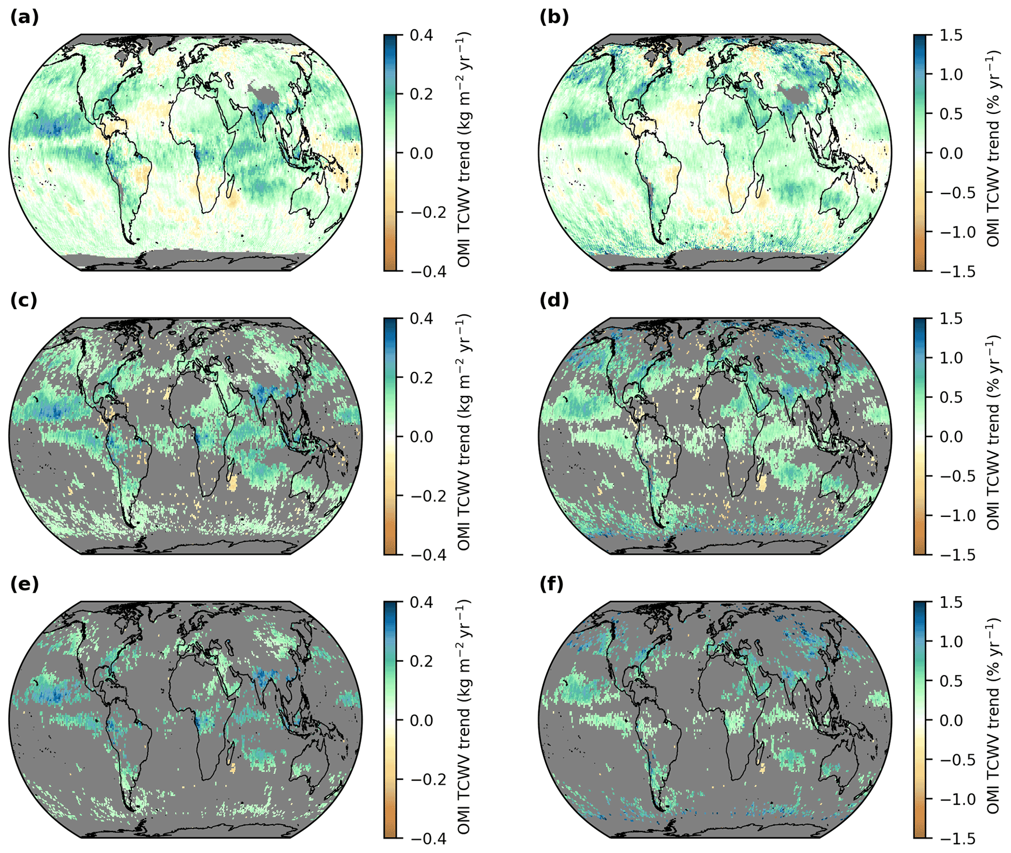
Figure 2 Global distributions of TCWV trends (2005–2020) derived from the MPIC OMI TCWV data set. Panels (a) and (b) depict the calculated absolute and relative TCWV trends, respectively. Panels (c) and (d) depict significant absolute and relative trends, respectively, after the application of the Z test. Panels (e) and (f) depict significant absolute and relative trends, respectively, after the application of the Z test and the false discovery rate (FDR) test. Grid cells for which no trend could be calculated (a, b) and/or for which the trends do not fulfil the significance criteria (c–f) are coloured grey.
The top row shows the absolute trends b (Fig. 2a) and the relative trends (Fig. 2b), respectively. Overall, increasing TCWV amounts are obtained. The absolute trends show high values in the equatorial Pacific and Southeast Asia, and the relative trends reveal high values in North America, the northern Pacific, and Southeast Asia. However, negative values in the TCWV trends can also be observed, e.g. in the region of the South Pacific convergence zone, southern Africa, Brazil, and the equatorial Atlantic. Altogether, we obtain a global area-weighted (i.e. weighted by the cosine of the latitude) mean absolute TCWV trend of +0.054 kg m−2 yr−1 and a relative TCWV trend of approximately +0.21 % yr−1. We also obtained distinctively high trend values over mountains such as the Himalayas and Andes. However, these high values are likely artefacts due to uncertainties of the satellite retrieval, for example, in the input data for the ground elevation. Thus, we decided to filter these artefacts and only show grid cells for which the mean ground elevation is lower than 3000 m above mean sea level, based on the GMTED2010 elevation data set (Danielson and Gesch, 2011).
The linear least squares fit assumes that errors of the estimators are normally distributed. Thus, we can perform a Z test from the fit results and determine which trends are statistically significant or not. For our purposes, we choose a significance level of 5 %, for which the Z test requires that |b|≥1.96σb (see Fig. 2c and d). Furthermore, to account for test multiplicity and field significance, we additionally perform a false discovery rate (FDR) test (Benjamini and Hochberg, 1995; Wilks, 2006, 2016). Because the OMI TCWV data set also shows a high spatial autocorrelation (see Appendix B), we follow the recommendations in Wilks (2016) and choose a significance level of 2.5 % for the FDR test.
The remaining trends are given in the bottom row of Fig. 2, with the absolute and relative trends in panels (e) and (f), respectively. From about 12 500 trends originally classified as significant according to the Z test, approximately 4700 grid cells still remain significant after the application of the FDR test, and almost all of them reveal a positive TCWV trend, in particular over the Pacific Ocean, East Asia, and parts of the U.S. East Coast.
In addition to the TCWV trends, we also analyse the trends of the individual components of the DOAS retrieval, i.e. the slant column density (SCD) and the air mass factor (AMF), where TCWV = SCD/AMF. These additional analyses reveal that the TCWV trends are mainly determined by trends in the SCD, i.e. by increasing or decreasing H2O absorption due to changing atmospheric water vapour content, respectively. The trends of the inverse AMF (i.e. 1/AMF) are generally negative but also distinctively weaker (about 3–4 times) than the SCD trends and thus have only a moderate influence on the overall TCWV trends. More details on these analyses are given in Appendix C.

Figure 3 Global distributions of TCWV trends (2005–2020) derived from the MPIC OMI TCWV data set. Panels (a) and (b) depict the calculated relative TCWV trends with and without teleconnection indices, respectively, in the trend analyses. Panel (c) depicts the differences between the trend results with teleconnections in the analysis minus the trend results without teleconnections in the analysis. Grid cells for which no trend could be calculated are coloured grey.
To highlight the influence of teleconnections on the trend results for the OMI TCWV data set, we also perform the trend analysis not accounting for them. The resulting trends and their difference are shown in Fig. 3. While overall the spatial distributions of the relative trends (Fig. 3a and b) look quite similar, distinct patterns emerge when looking at the trend difference (Fig. 3c). For instance, the typical PMM and ENSO teleconnection patterns are clearly visible (e.g. dipole structure over the maritime continent in the case of ENSO). Consequently, the resulting deviations are particularly strong in the tropical and subtropical Pacific and can reach values as high as the relative trends themselves. We have also tested other AR models with lag =2, 3, 6, and 12 and found that the trend results and the distributions of the significant trends differ only slightly from those using an AR(1) model. The corresponding trend results can be found in Fig. S2 in the Supplement.
3.2 Intercomparison to trends of other TCWV data sets
To verify the OMI TCWV trends and to detect potential shortcomings within the OMI TCWV data set, we performed the analyses also for monthly mean TCWV data from the reanalysis model ERA5 (Hersbach et al., 2019, 2020). For this purpose, the ERA5 TCWV data set is gridded on a lattice. Moreover, to account for OMI's observation time (13:30 LT), we only take into account ERA5 monthly mean values between 13:00–14:00 LT.
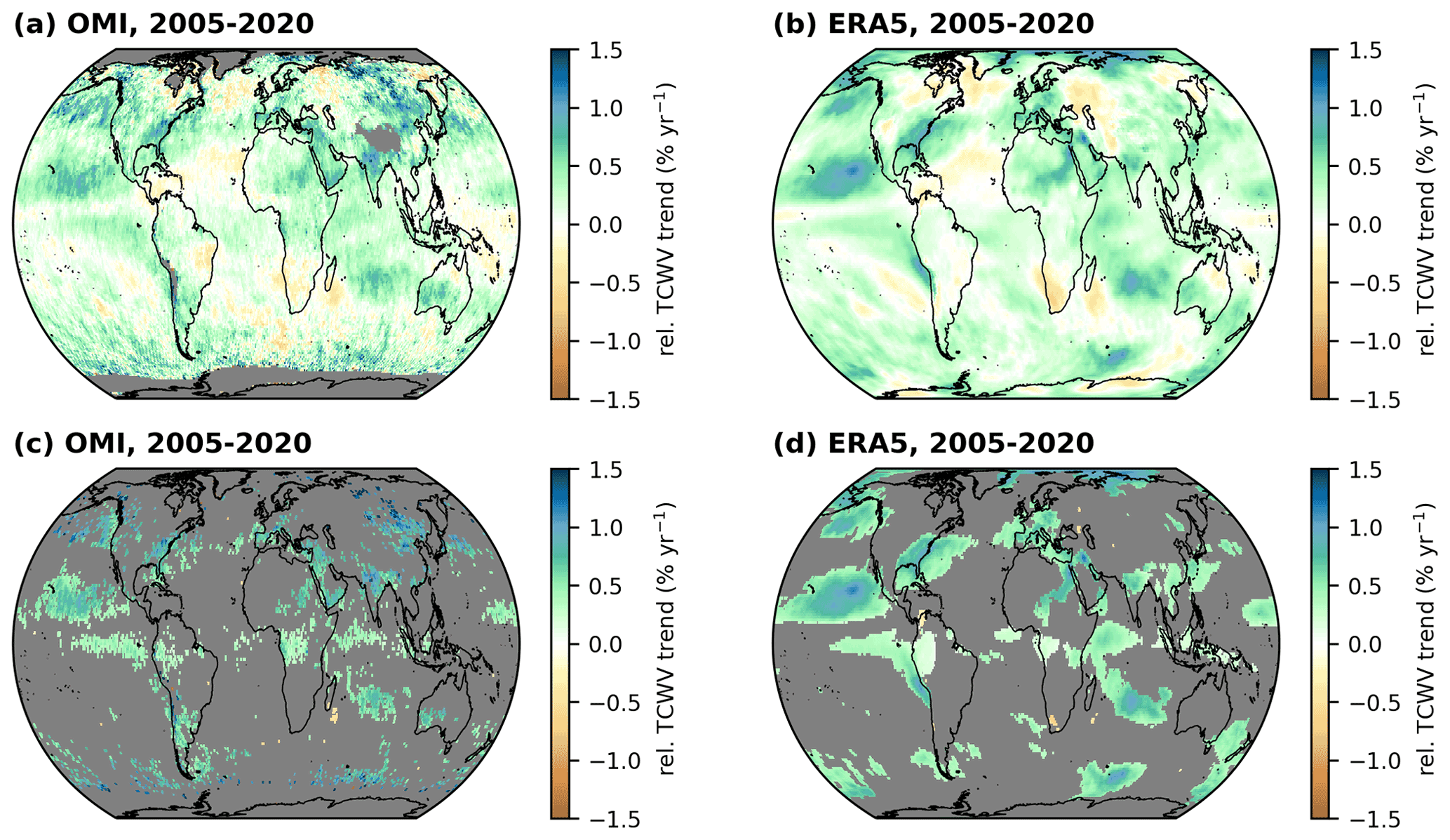
Figure 4 Global distributions of relative TCWV trends derived from the OMI TCWV data set (a, c) and ERA5 (b, d). Panels (a) and (b) depict all calculated relative TCWV trends, and panels (c) and (d) show the corresponding significant trends remaining after the application of the Z test and FDR test. Grid cells for which no valid trend could be calculated are coloured grey.
The resulting maps of the relative trends are given in Fig. 4. Overall, the trend results of OMI and ERA5 agree well to each other, as both all and only significant relative trend results (top and bottom rows in Fig. 4, respectively) have similar strengths and also show similar global distributions. Nevertheless, the OMI TCWV trends reveal slightly stronger increases over parts of East Asia (which are also classified as significant) and South America and are in general less smooth than the ERA5 results. Similar findings can be obtained for the absolute trends, which are available in Fig. S3 in the Supplement.

Figure 5 Global distributions of relative TCWV trends derived from the OMI TCWV data set (a, c) and GOME-Evolution (b, d) for the time range from January 2005 to December 2015. Panels (a) and (b) depict all calculated relative TCWV trends, and panels (c) and (d) show the corresponding significant trends remaining after the application of the Z test and FDR test. Grid cells for which no valid trend could be calculated are coloured grey.
In addition to ERA5, we also compare the trend results to trends from the TCWV satellite product GOME-Evolution (Beirle et al., 2018). Since the GOME-Evolution product is only available until 2015, we modified the time range accordingly, i.e. the results for the relative trends shown in Fig. 5 (and for the absolute trends in Fig. S4) correspond to a time range from January 2005 to December 2015. While the distributions of the relative trends have quite similar patterns and partly similar magnitudes, striking differences can be seen in some regions. For example, the OMI trends in the tropical Pacific North America or the Arabian Peninsula are much higher than the GOME-Evolution trends. Also, overall, many more trends are classified as significant for OMI than for GOME-Evolution.
Nevertheless, considering that the GOME-Evolution product retrieves total column water vapour in the visible red spectral range, uses a different vertical column density (VCD) conversion scheme (see also Wagner et al., 2003, 2007; Grossi et al., 2015), and observes the atmosphere at an earlier overpass time (around 10:00 LT), the good agreement in the trend results further confirms the reliability of the findings of the OMI TCWV trend analysis.
Furthermore, we made additional comparisons to the results of past studies. From these comparisons, several differences in the strength and spatial distribution of TCWV trends emerge. The reasons for these differences are, on the one hand, the consideration of different time periods and, on the other hand, also different methods of analysis. Further details about these comparisons can be found in Appendix D.
In this section, we investigate to what extent the assumption of constant relative humidity is given at the local scale. For this purpose, we make the following assumptions. First, we assume that the relative changes in TCWV correspond to those in near-surface specific humidity qs, i.e. . This assumption should be fulfilled, since TCWV is directly connected to the specific humidity via its vertical integral, and approximately 60 % of the TCWV is located within the planetary boundary layer. Second, we also assume that relative changes in specific humidity correspond to changes in water vapour pressure, i.e. (assuming that relative changes in surface air pressure are negligible, i.e. ). Given the aforementioned assumptions and that the water vapour pressure e can be described as , we can derive the relative changes in relative humidity (RH) by combining the relative TCWV trends with trends in surface air temperature T, as follows:
Thus, if RH is 50 %, a relative increase of 1 % indicates an absolute RH increase of 0.5 %. However, it should be noted that the largest uncertainties lie in the first assumption, i.e. slight under- or overestimations of the actual relative qs changes will cause corresponding deviations in the relative RH changes.

Figure 6 Relative trends in relative humidity (RH) derived from the relative TCWV trends and the temperature trends from OMI and Berkeley Earth (a), from ERA5 (b), and from the data set HadISDH (Hadley Centre Integrated Surface Dataset of Humidity) (c) for the time range from January 2005 to December 2020. Grid cells for which no trend has been calculated are coloured grey.
Figure 6 depicts the resulting relative RH trends derived from the OMI TCWV trends in combination with the temperature trends from the Berkeley Earth temperature data record (Rohde and Hausfather, 2020), from ERA5, and from the relative RH trends from the HadISDH (Hadley Centre Integrated Surface Dataset of Humidity) surface relative humidity data set (Willett et al., 2014, 2020). In general, the results for OMI and ERA5 reveal a global (relative) increase in RH, in particular that the trends over ocean are widely positive. However, in all three data sets, distinctive decreasing trends are observable over land, for instance over Russia or southern Africa. Considering the differences in the selected time period and measurement source, the RH trends from OMI over land surface coincide well with the results from Dunn et al. (2017). The reduction in relative RH over land is likely related to a marked land–ocean contrast in warming (Simmons et al., 2010; Fasullo, 2012), besides various local factors such as changes in vegetation cover (Simmons et al., 2010). Over ocean, due to the direct link with sea surface temperature, the water vapour content can increase adequately to keep RH constant. Over land, this is usually only possible with a delay due to limited water availability, as water must first be transported there from ocean. Since the temperature also increases much more over land than over ocean, the decrease in RH might be due to the lack of an increased water supply from the ocean (Simmons et al., 2010).
Interestingly, we also find distinctive increases in RH in arid regions (e.g. over the Sahara) and distinctive decreases in humid regions (e.g. the tropical Pacific Ocean) within the OMI and the ERA5 results. Recently, Bourdin et al. (2021) investigated RH trends from the reanalysis models ERA5 and JRA-55 (Japanese 55-year Reanalysis) over the past 40 years and also found significant negative trends in the tropical lower troposphere.
Several studies have shown that global warming will lead to a further drying of dry regions (e.g. Sherwood and Fu, 2014), and wet regions will become even wetter (e.g. Held and Soden, 2006; Chou et al., 2013; Allan et al., 2010), leading to the simple paradigm of “dry gets drier, wet gets wetter” (DDWW; Chou et al., 2009). In addition, other studies show that changes in precipitation correlate very well with changes in ocean salinity, suggesting a “fresh gets fresher, salty gets saltier” pattern (Cheng et al., 2020, and references therein). Though most of these studies focus on changes in precipitation, our results for RH support the findings from Greve et al. (2014) and Byrne and O'Gorman (2018) in that the DDWW paradigm is not always fulfilled over land. Surprisingly, according to our results, this paradigm is not fulfilled even over the tropical Pacific Ocean, the region on which most of the concepts of the studies are based (e.g. Held and Soden, 2006). However, we would like to stress here that the time period studied is probably too short to question the paradigm.
According to Bretherton et al. (2004) and Rushley et al. (2018), a nonlinear relationship between TCWV (or column relative humidity, respectively) and precipitation exists for the tropical ocean. Thus, given the TCWV and RH trend results, we expect to observe a decline or negative trend, in particular over the Pacific Ocean, along the Intertropical Convergence Zone. For the analysis of trends in precipitation, we use the monthly mean rain rates from the GPCP Version 3.2 Satellite-Gauge (SG) Combined Precipitation Data Set (Huffman et al., 2020). For the sake of consistency, we grid the GPCP data from a resolution of to a lattice.
Although precipitation climate data records (CDRs) allow a global analysis, they are subject to large uncertainties, as satellite and rain gauge observations do not have good spatiotemporal coverage, weak and short rain events are not well detected or even missed, and satellite retrievals can determine the rain rate only indirectly. Thus, deviations of about 50 % in the daily rain rate can occur, compared to in situ measurements (e.g. Prat et al., 2021). Nevertheless, Prat et al. (2021) show that, over accumulation periods of month or years, precipitation CDRs perform satisfactorily. Moreover, Prat et al. (2021) used an older GPCP version (v2) than ours in their evaluation study.
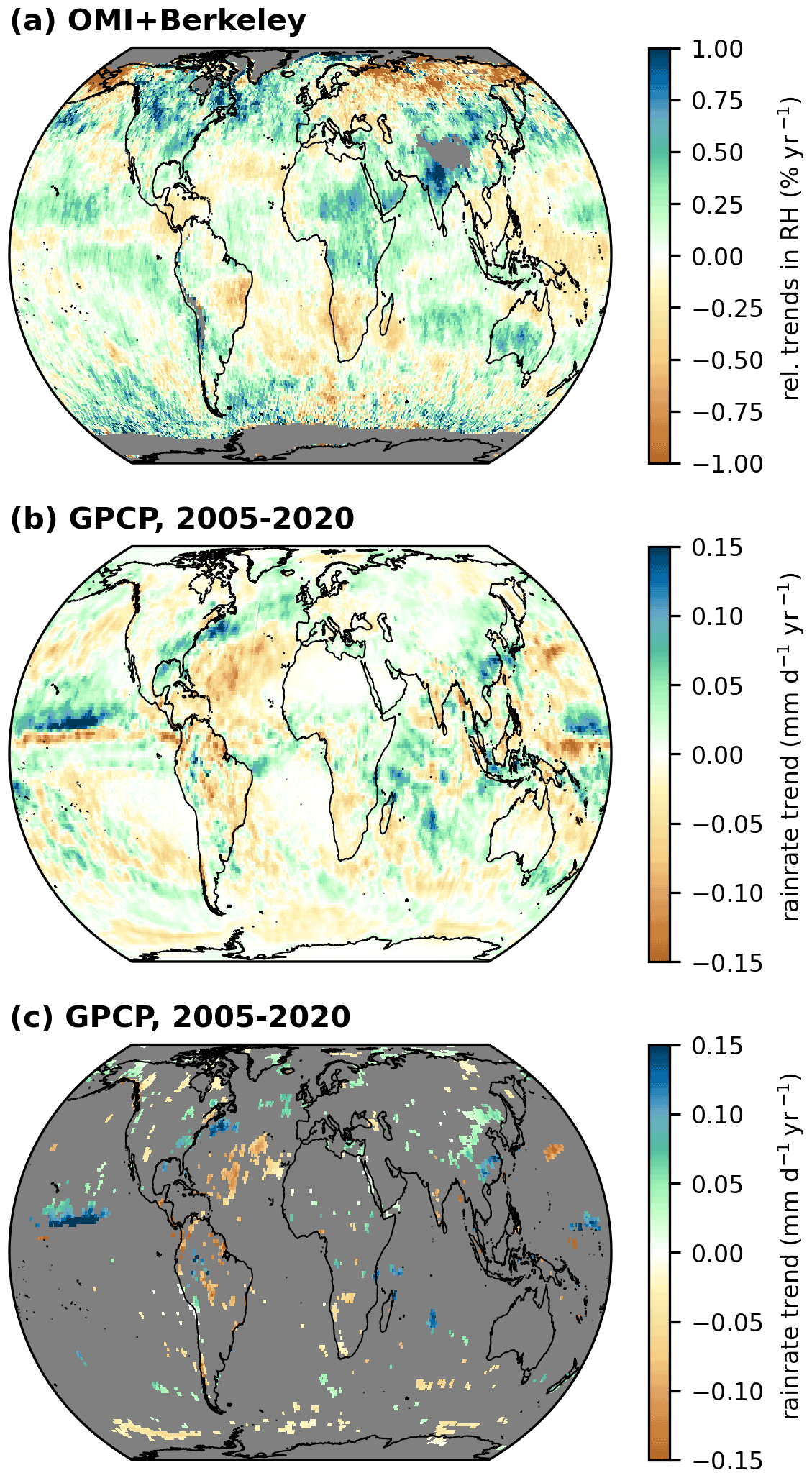
Figure 7 Global distribution of relative RH trends derived from the OMI TCWV data set (time range from 2005 to 2020; a; same as in Fig. 6a) and of trends in precipitation derived from the GPCP v3.2 monthly mean data set for the time range from January 2005 to December 2020. Panel (b) depicts all rain rate trends, and panel (c) shows only those that are considered significant after applying the Z test (to the significance level of 5 %) and a FDR test (see also Appendix B). Grid cells for which no valid trends have been calculated are coloured grey.
Figure 7 depicts the obtained trends in precipitation and the relative RH trends from OMI. Comparing the trend distributions of the monthly mean rain rates to the relative RH trends, negative and positive trends in precipitation and RH match quite well over the tropical and subtropical ocean, especially over the tropical Pacific and the northern subtropical Atlantic. While over land within the subtropics an acceptable match can be determined in some regions (e.g. southern Africa and Brazil), the patterns of the relative RH and rain rate trends no longer match well towards mid and high latitudes (e.g. in North America), likely because, in these regions, the rain rate is mainly determined by atmospheric dynamics (cyclone or storm tracks) rather than thermodynamics. Furthermore, the distinctive relative increases in RH in the mountainous regions of South America (Andes) and northern India (Himalayas) are likely due to the inadequacies in the OMI TCWV satellite data caused by the complex topography (see also Sect. 3.1).
Trenberth (2011) and Trenberth and Shea (2005) analysed local correlations between precipitation and surface temperature for cold and warm seasons and reported mainly positive correlations over ocean and negative correlations year round over land throughout the tropics. However, over ocean, the correlations also depend on whether the (sea) surface temperature is driven by the ocean or by the atmosphere (Trenberth and Shea, 2005). While in some regions of the subtropics we can also find this high correlation in the trend patterns of precipitation and surface temperature (e.g. increase in the precipitation in the northern subtropics in the eastern Pacific or decrease in the subtropical Atlantic over ocean; decrease in Brazil or southern Africa over land), we cannot find a direct link for the striking negative precipitation trends in the equatorial Pacific. However, it should also be taken into account that a large part of the precipitation trends are not statistically significant.
Overall, the discrepancies between our observations and the expected changes in the hydrological cycle show that accurate observations and long-term monitoring of the Earth's hydrological cycle and atmosphere on the global scale from multiple remote sensing and in situ platforms are essential to clarify this important aspect.
Another key diagnostic of the hydrological cycle is the atmospheric water vapour residence time (WVRT). The WVRT can contribute to a better understanding of changes in dynamic and thermodynamic processes within a changing climate (Trenberth, 1998; Gimeno et al., 2021). For instance, an increase in WVRT suggests that the length of the atmospheric moisture transport increases, i.e. the distance between moisture sink and source regions (Singh et al., 2016). Several different metrics exist for quantifying the WVRT (van der Ent and Tuinenburg, 2017; Gimeno et al., 2021), bearing in mind that the WVRT distribution or the lifetime distribution (LTD) is exponential on the local scale, and thus, the mean value is strongly influenced by a few high values (van der Ent and Tuinenburg, 2017; Sodemann, 2020). Ideally, one would determine the LTD for each grid cell for each month from backward trajectories and then examine their changes or trends. However, this would be well beyond the scope of this paper.
Thus, for our purpose, and for the sake of simplicity, we focus on the so-called depletion time constant (DTC) and the turnover time (TUT). The TUT describes the global average mean age of precipitation and can be calculated as the ratio of TCWV to precipitation P, as follows:
where the bar indicates global average. Typically, the TUT varies between values of 8 to 10 d and is expected to increase by 3 % K−1–6 % K−1 (Gimeno et al., 2021, and references therein). Analogously, the DTC is defined as the local ratio of TCWV to precipitation, as follows (e.g. Trenberth, 1998):
The DTC values might vary substantially from TUT, but the global precipitation weighted average is equal to TUT (Gimeno et al., 2021).
For our investigations of trends in DTC, we combine the regridded GPCP data set from Sect. 4 and the OMI TCWV data set and perform the trend analysis scheme from Sect. 2.2 to the monthly DTC values for the time range 2005 to 2020. To ensure numerical stability, we only consider monthly rain rates greater than 0.25 mm d−1. As a result, large parts of the subtropical oceans and deserts are excluded from the analysis.
The results of the DTC trend analyses are depicted in Fig. 8. On average, we typically obtain mean DTC values between 5–10 d in the areas where rain occurs (Fig. 8a). In the subtropical dry zones, values of around 30 d and well above are found. In terms of absolute DTC trends, the most striking patterns are in the northern subtropical Atlantic, with strong increases, and in the northern subtropical western Pacific, with strong decreases. In comparison, the distribution of relative DTC trends is much spottier, but overall, in addition to the patterns already mentioned, we obtain distinctive increases in DTC on the U.S. West Coast, in Europe, Russia, and in the eastern Pacific.
For our investigations of trends in TUT, we first calculate global averages of the regridded GPCP data set from Sect. 4 and the OMI and ERA5 TCWV data sets between 60∘ S and 60∘ N for each month, then combine the time series of global averages, and, finally, perform the trend analysis for the TUT time series for the time range from 2005 to 2020.
Altogether, we find an increase in the global TUT for OMI and ERA5 of approximately +0.02 d yr−1, with TUT mean values of around 9.7 d for OMI and 8.8 d for ERA5. Combining the long-term relative trends in TUT and trends in surface air temperature, we can estimate the sensitivity of TUT to global warming r, i.e. . For the case of OMI and Berkeley Earth, we find a TUT sensitivity of around 8.4 % K−1 and for ERA5 of around 8.8 % K−1, which is higher than the results of 3 % K−1–6 % K−1 pooled in Gimeno et al. (2021).

Figure 8 Global distribution of DTC trends for the time range of January 2005 to December 2020. Panel (a) depicts the distribution of the mean DTC. Panels (b) and (c) depict the absolute and relative DTC trends. Grid cells for which no valid trend has been calculated are coloured grey.
In this study, we analysed global trends within a long-term data set of total column water vapour (TCWV) retrieved from multiple years of OMI observations for the time period January 2005 until December 2020 and considered the effects of autocorrelation of the residuals within the analysis scheme. The results of the analyses were then put into context with trends from additional TCWV data sets, like from the GOME-Evolution project or from the reanalysis model ERA5, and overall very good agreement was found. In a next step, based on the relative OMI TCWV trends, trends in relative humidity were derived and put into the context of the assumption of invariant relative humidity. Moreover, under consideration of the relationship between (column) relative humidity and precipitation, the patterns of the relative RH trends have been compared to rain rate trends. Also, the changes in the water vapour residence time and its response to changes in surface air temperature were investigated.
The trend analysis reveals an increase in TCWV of approximately +0.054 kg m−2 K−1 or +0.21 % yr−1 globally for the time period of January 2005 until the end of 2020. To determine if trends are significant or not, a Z test and a false discovery rate test are applied to the trend results. After application of these significance criteria, almost all remaining trends are positive and distributed across the globe. However, particular spatial patterns remain, for instance within the region of the northern subtropics of the eastern Pacific. Overall, the relative OMI TCWV trends agree well to the corresponding trends from ERA5 and from the GOME-Evolution data set.
To analyse if the assumption of temporally invariant relative humidity is fulfilled on the local scale, we derived relative trends in relative humidity (RH) from the TCWV trends. All in all, we obtain that RH increases distinctively over large areas of the ocean and land surface. However, over both surface types relative decreases can also be well identified in some areas. Interestingly, relative decreases and increases in RH are not limited to arid and humid regions, respectively. For instance, our analysis reveals relative increases in RH over the (arid) Sahara desert and decreases in RH over the (humid) tropical Pacific Ocean. Within the tropics, we also find that the patterns of decreasing RH trends match those of decreasing precipitation quite well, especially within the tropical Pacific Ocean.
Combining the TCWV and rain rate data sets, changes in the water vapour residence time (WVRT) have been investigated. Overall, an increase in the turnover time of about 0.02 d yr−1 has been observed. Together with the long-term trends in surface temperature, we estimate a TUT sensitivity to global warming of around 8.4 % K−1, which is 2 to 3 times higher than the values provided in Gimeno et al. (2021).
All in all, our results show that several challenges still remain for a better understanding of the atmospheric hydrological cycle and even new questions arise regarding the complex interactions between air temperature, water vapour, precipitation, and atmospheric dynamics. The differences between observed and expected changes in the hydrological cycle show that simplified assumptions are not always valid (e.g. invariant relative humidity). Also, our observed, much higher global sensitivities of individual parameters of the hydrological cycle (i.e. TUT) to changes in surface temperature raise the question of what effects can be expected at the local scale (e.g. precipitation) with further increasing temperatures, especially with regard to changes in the global circulation such as the expansion of the Hadley cell towards higher latitudes (e.g. Staten et al., 2018).
With regard to TCWV retrievals in the visible blue spectral range, there is great potential for extending the OMI TCWV data set with further satellite data (e.g. from TROPOMI or GOME-2) and combining it with future missions from geostationary satellites, such as GEMS or Sentinel-4, which will also allow for investigations of (semi-)diurnal TCWV cycles.
To address the influence of the autocorrelation on the trend results for the OMI TCWV data set, we perform the trend analysis not accounting for it. The panels in Fig. A1 illustrate the difference in the absolute (Fig. A1a) and relative (Fig. A1b) trend results (i.e. the difference of the results with accounting minus the results without accounting for the influence of the temporal autocorrelation). For high and mid latitudes, the differences are close to zero, indicating that the influence of the autocorrelation on the trend results is negligible. However, within the subtropics and tropics, distinctive deviations are observable, especially in the regions where the autocorrelation is high (e.g. the Pacific Ocean; see also Fig. 1). For the case of the relative trends (Fig. A1b), the deviations can reach up to 0.05 % yr−1 (which is around 10 % of the magnitude of the relative trends in the affected regions) and consequently can cause wrong signs in the trend estimation (i.e. indicating a negative instead of a positive trend).
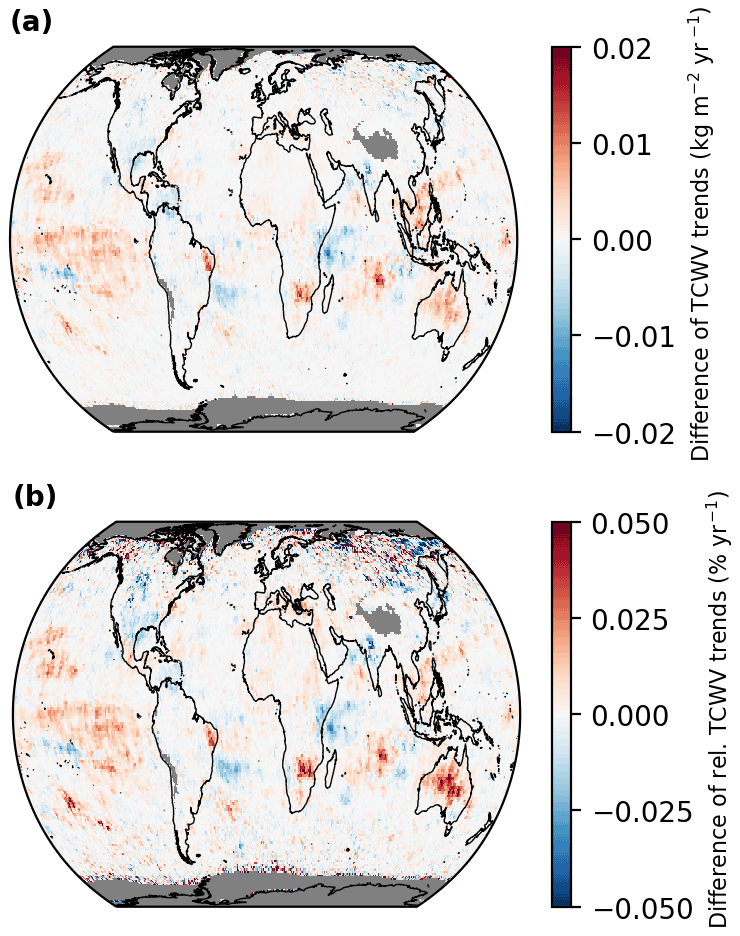
Figure A1 Difference between trends of the MPIC OMI TCWV data set (2005–2020) with accounting minus not accounting for the influence of autocorrelation, where panel (a) shows the absolute trends and panel (b) the relative trends.
The significance level at which the false discovery rate test method in Sect. 3.1 is performed depends on the degree of spatial autocorrelation. Thus, for every timestamp within the MPIC OMI TCWV data set, the spatial autocorrelation is calculated from the global TCWV distribution for grid point separations up to 7000 km.
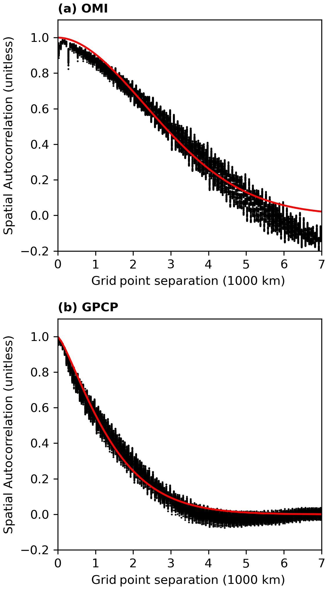
Figure B1 Spatial autocorrelation as function of the great circle distance of the MPIC OMI TCWV (a) and the GPCP data set (b). The black dots represent the results of the analysis of the spatial distribution for each time step in the respective data set. The solid red lines illustrate the fit result of .
Figure B1a illustrates the spatial autocorrelation of the OMI TCWV data set as a function of grid point separation. The red solid line is the fit result of , with the grid point separation distance x. For the OMI TCWV data set, we calculated a value of a≈0.098 and b≈1.88, which equals an e-folding distance of approximately 3.43×10³ km. According to Wilks (2016), this e-folding distance indicates a strong spatial dependency. Consequently, we follow the recommendations of Wilks (2016) and set, for the FDR test, the significance level to 2.5 % instead of 5.0 %.
The same procedure was applied to the GPCP data set, the results of which are shown in Fig. B1b. For the fit results, we obtain a≈0.58 and b≈1.28, which correspond to an e-folding distance of 1.53×10³ km, which is thus less than half as large as that of TCWV. Accordingly, the spatial dependence is not so strong, and the significance level for the FDR test can remain at 5 % for the GPCP data set.
Here, we investigate to what extent the relative TCWV trends are due to geophysical changes in the water vapour content or due to changes in the retrieval input parameters. For DOAS retrievals, the TCWV amount is derived via the quotient of the integrated concentration along the light path (so-called slant column density, SCD) and the so-called air mass factor, AMF, i.e. TCWV = SCD/AMF. Thus, the relative trends of these two quantities were calculated following the analysis scheme in Sect. 2.2. For the case of the SCD, we use the geometrical VCD (vertical column density), which is simply the SCD divided by the geometrical air mass factor (which remains constant over time).
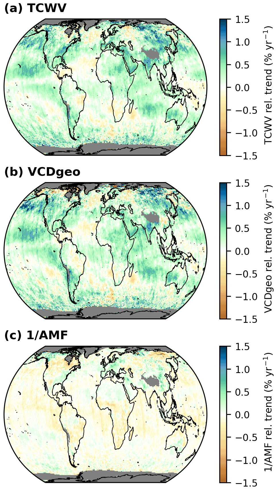
Figure C1 Global distributions of relative trends of the TCWV (a), geometrical vertical column density (VCDgeo; b), and the inverse of the air mass factor (1/AMF; c) for the time period from January 2005 to December 2020. Grid cells for which no trend has been calculated are coloured grey.
The global distributions of the relative trends of both quantities are illustrated in Fig. C1b and c and the relative TCWV trends (in Fig. C1a). The distribution and strength of the geometrical VCD (Fig. C1b) largely coincide with the distribution of the relative TCWV trends (Fig. C1a). The trends of the inverse AMF (1/AMF, Fig. C1c), on the other hand, are, in general, much weaker than the SCD trends (approx. 3–4 times weaker) and do not follow the TCWV trend distribution. However, it occasionally happens that the relative inverse AMF trends either weaken or cancel the SCD trends (e.g. North America or northeastern Asia) or even strengthen them (e.g. around the Arabian Peninsula). Overall, we conclude that the relative TCWV trends are mainly determined by the SCD trends, which consequently means that TCWV trends are mainly due to an increase in atmospheric water vapour concentration.
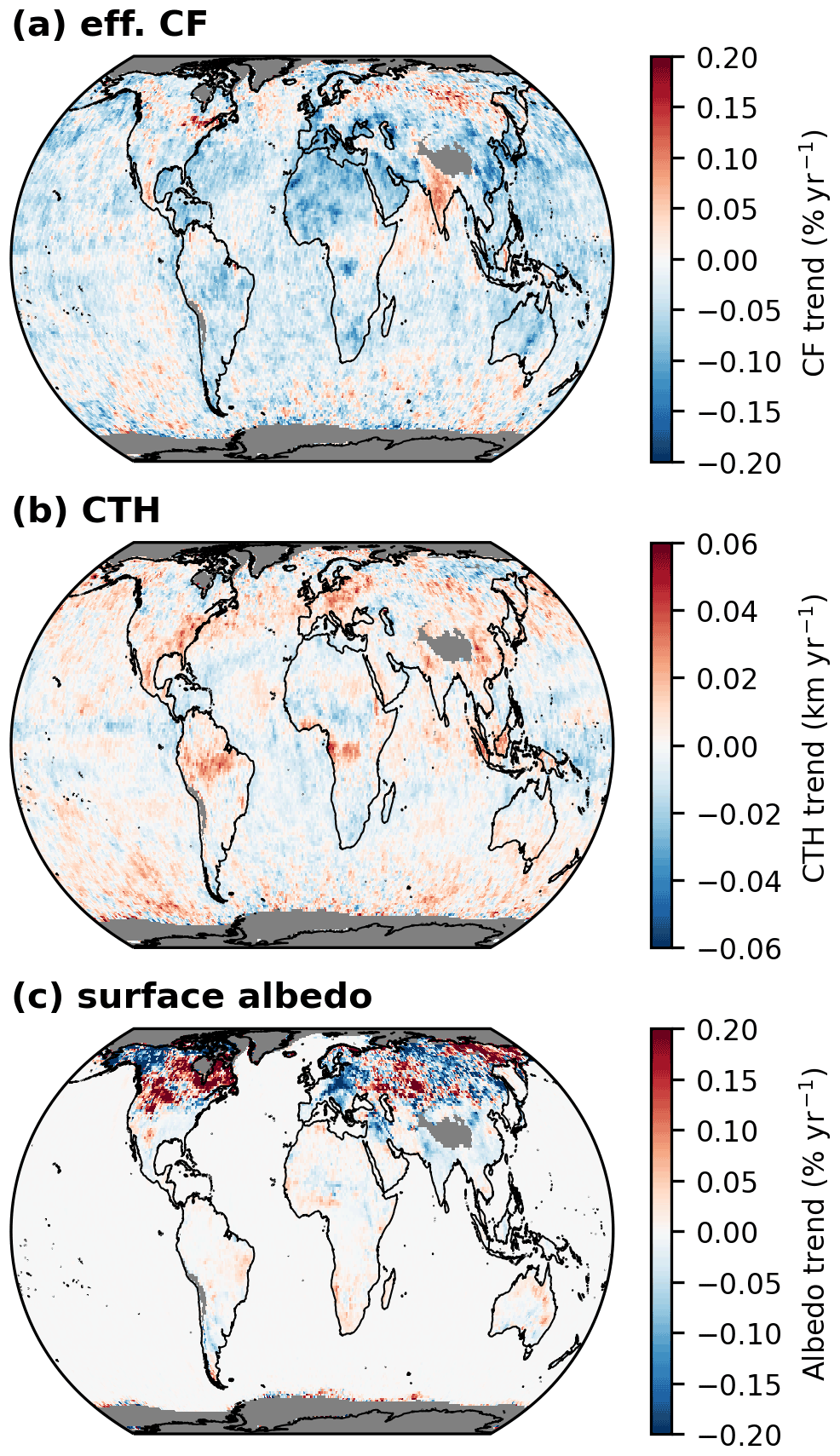
Figure C2 Absolute trends of the retrieval input parameters for the calculation of the air mass factor for the time period from January 2005 to December 2020. (a) Effective cloud fraction. (b) Cloud-top height. (c) Surface albedo. Grid cells for which no trend has been calculated are coloured grey.
In addition to the trends of the SCD and AMF, we also analyse the trends of the AMF input parameters, i.e. the effective cloud fraction (CF), the cloud-top height (CTH), and the surface albedo. The corresponding global distributions are depicted in Fig. C2. Here, it is important to mention that the MPIC OMI TCWV data set only includes mostly clear-sky observations (i.e. CF <20 %), so the calculated trends of the cloud input parameters are very likely not representative for the actual cloud trends of the atmosphere. For CF (Fig. C2a), we obtain, in general, decreasing trends around −0.1 % yr−1 globally, except for the Indian subcontinent and some individual locations. For the input CTH (Fig. C2b), no clear trend pattern is observable, except for slight increasing trends over the tropical landmasses with values around +0.03 km yr−1. As expected for the surface albedo (Fig. C2c), no trends are observable over ocean, as a static monthly albedo map has been used here. Over land, however, strong varying trends can be found in the high latitudes of the Northern Hemisphere, with absolute values higher than 0.2 % yr−1. Nevertheless, these strong albedo trends in the Northern Hemisphere are typically not significant.
In the following, we compare our results of relative TCWV trends for the time range 2005–2020 to trends presented in previous studies and investigate which TCWV trends are significant within the respective time range of the previous studies. It is particularly important to note that TCWV trends from different time periods have been investigated. For the sake of completeness, the global distributions of the absolute trends for the same data sets and time ranges are available in Fig. S5 in the Supplement.
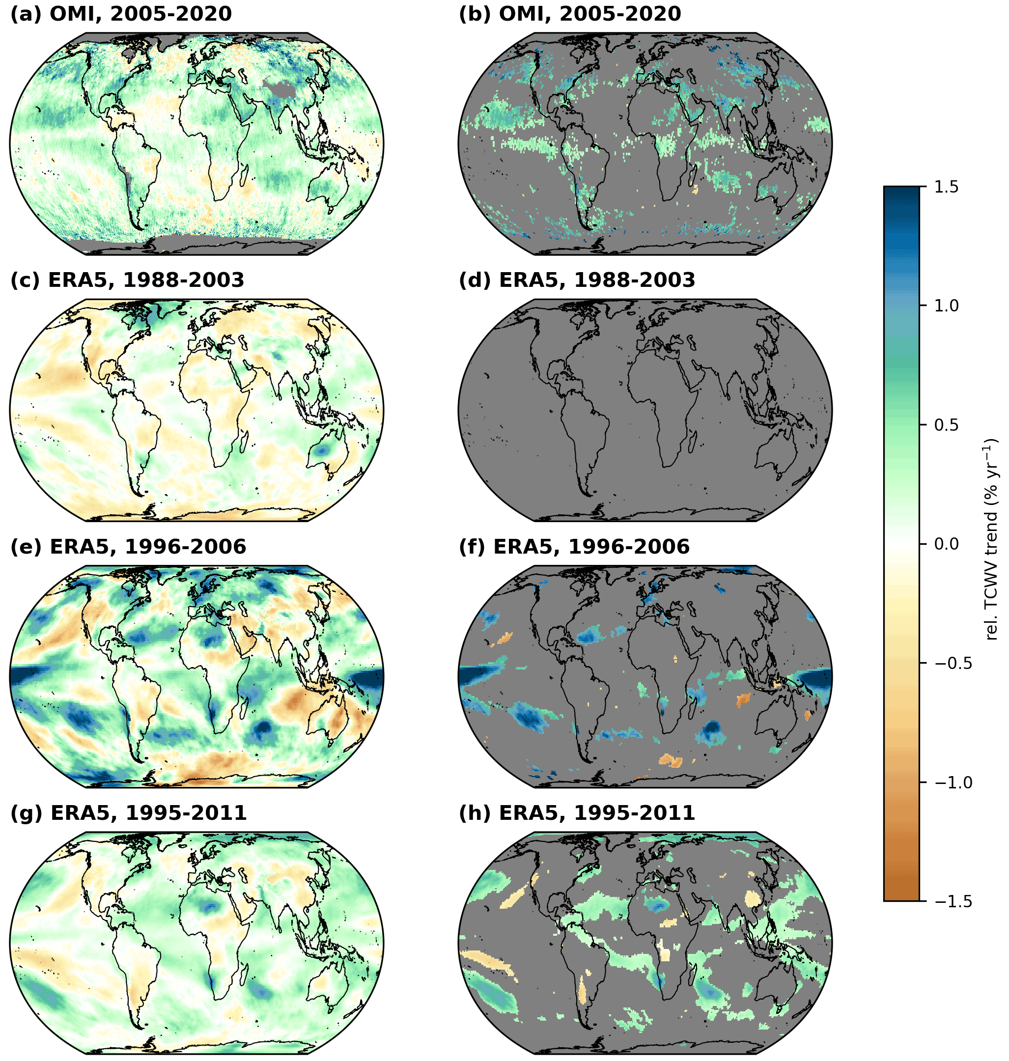
Figure D1 Global distributions of relative TCWV trends of OMI (2005–2020; a, b) and ERA5 for the following different time periods: (c, d) 1988–2003, (e, f) 1996–2006, and (g, h) 1995–2011. Panels in the left column illustrate all calculated trends, and panels in the right column illustrate statistically significant trends after the application of a Z test and a FDR test. Grid cells for which no valid trend has been calculated are coloured grey.
Trenberth et al. (2005) analysed trends from the RSS SSM/I data for the time period of 1988 to 2003. While the patterns generally match quite well, the trends often have opposite signs. In our period (2005–2020), the trends are mainly positive, whereas in the period of this study (1988–2003), the trends are mainly negative. This is particularly visible in the eastern Pacific. However, we were unable to identify any significant trends for this period (see Fig. D1d). Overall, however, the trends of Trenberth et al. (2005) are in very good agreement with the trends we have determined for this period (compare Fig. 11 in their paper).
Mieruch et al. (2008) investigated TCWV trends from 1996 to 2006, using a TCWV data set created from measurements of GOME and SCIAMACHY, using the AMC-DOAS method (Air Mass Corrected Differential Optical Absorption Spectroscopy; Noël et al., 2004). In contrast to the comparison with Trenberth et al. (2005), almost no similarities are discernible either in the spatial patterns or in the strength of the trends. Overall, the spatial distribution is not as smooth as in the other periods studied and is distinctively spottier. This is probably due to the fact that the period studied is quite short and that there was also a strong El Niño event in 1997/1998. Compared to the results in Mieruch et al. (2008, Fig. 5 in their paper), our results for the same period find only few similarities, even for the case of the significant trends. For example, the trends of Mieruch et al. (2008) are sometimes 4 to 6 times higher than ours for the same period.
More recently, Wang et al. (2016) also investigated TCWV trends for the time period from 1995 to 2011 for a TCWV data set combining measurements from radiosondes, GPS radio occultation, and microwave satellite instruments. As for the comparison to Trenberth et al. (2005), our findings and the findings from Wang et al. (2016) share many similarities but also several discrepancies. Wang et al. (2016) find a “sandwich” shape in the tropical and subtropical Pacific, with positive trends in the region of the Intertropical Convergence Zone bounded by two bands of negative trends. In contrast, the OMI TCWV trends also suggest a sandwich shape but with opposite signs to Wang et al. (2016), i.e. negative trends bounded by positive trends. Such opposite findings also occur over parts of the Indian subcontinent, the Arabian Peninsula, and South America. However, for central Europe and parts of Asia, good agreement for the trend patterns is found.
For the comparisons of our results to the findings of Trenberth et al. (2005), Mieruch et al. (2008), and Wang et al. (2016), one explanation for the differences may be the different time periods of investigations (1988 to 2003, 1996 to 2006, and 1995 to 2011 vs. 2005 to 2020). Figure D1c–h illustrate the relative TCWV trends derived from the ERA5 data set for the aforementioned time periods. Although only the time periods have been changed, clear differences can indeed be identified in both the distribution and the strength of the trends. Furthermore, these trend distributions agree very well with the results of the three previously mentioned studies. Nevertheless, different methodologies of observations or different methods for the trend calculation may also be a cause for the discrepancies. For instance, we explicitly account for the influence of ENSO by including the ONI and TNI index into our analysis scheme (see also Sect. 2.2 and Sect. 3.1), whereas Mieruch et al. (2008) explicitly filtered the time around the strongest ENSO signal.
Combining that the detected trends for ERA5 and the GOME-Evolution data set agree well to the findings from the OMI TCWV data set (see Sect. 3.2) but that the comparisons to the results from other trend analysis studies show systematic differences, it is evident to not only compare trends for the same time periods but also to ensure that the same methodology for the trend analysis is used. As a lot of different methods exist for estimating trends in environmental data sets, it would be particularly interesting to evaluate which trend analysis scheme performs best and should be recommended for future studies. However, such an evaluation study is beyond the scope of this paper.
The MPIC OMI total column water vapour (TCWV) climate data record is available at https://doi.org/10.5281/zenodo.5776718 (Borger et al., 2021b).
The supplement related to this article is available online at: https://doi.org/10.5194/acp-22-10603-2022-supplement.
CB performed all calculations for this work and prepared the paper, together with SB and TW. TW supervised this study.
At least one of the (co-)authors is a member of the editorial board of Atmospheric Chemistry and Physics. The peer-review process was guided by an independent editor, and the authors also have no other competing interests to declare.
Publisher's note: Copernicus Publications remains neutral with regard to jurisdictional claims in published maps and institutional affiliations.
This article is part of the special issue “Analysis of atmospheric water vapour observations and their uncertainties for climate applications (ACP/AMT/ESSD/HESS inter-journal SI)”. It is not associated with a conference.
The ERA5 data (Hersbach et al., 2019) were downloaded from the Copernicus Climate Change Service (C3S) Climate Data Store. The results contain modified Copernicus Climate Change Service information 2021. Neither the European Commission nor ECMWF is responsible for any use that may be made of the Copernicus information or data it contains. The Dutch–Finnish-built OMI is part of the NASA EOS Aura satellite payload. KNMI and the Netherlands Space Agency (NSO) manage the OMI project. We acknowledge NASA's Goddard Earth Sciences Data and Information Services enter (GES-DISC), for free access to the data.
This research has been supported by the Bundesministerium für Bildung und Forschung (grant no. FKZ 50EE1619).
The article processing charges for this open-access publication were covered by the Max Planck Society.
This paper was edited by Farahnaz Khosrawi and reviewed by Kevin Trenberth and Chunlüe Zhou.
Allan, R. P., Soden, B. J., John, V. O., Ingram, W., and Good, P.: Current changes in tropical precipitation, Environ. Res. Lett., 5, 025205, https://doi.org/10.1088/1748-9326/5/2/025205, 2010. a
Beirle, S., Lampel, J., Wang, Y., Mies, K., Dörner, S., Grossi, M., Loyola, D., Dehn, A., Danielczok, A., Schröder, M., and Wagner, T.: The ESA GOME-Evolution “Climate” water vapor product: a homogenized time series of H2O columns from GOME, SCIAMACHY, and GOME-2, Earth Syst. Sci. Data, 10, 449–468, https://doi.org/10.5194/essd-10-449-2018, 2018. a
Benjamini, Y. and Hochberg, Y.: Controlling the False Discovery Rate: A Practical and Powerful Approach to Multiple Testing, J. Roy. Stat. Soc. Ser. B, 57, 289–300, 1995. a
Bennartz, R. and Fischer, J.: Retrieval of columnar water vapour over land from backscattered solar radiation using the Medium Resolution Imaging Spectrometer, Remote Sens. Environ., 78, 274–283, https://doi.org/10.1016/S0034-4257(01)00218-8, 2001. a
Borger, C., Beirle, S., Dörner, S., Sihler, H., and Wagner, T.: Total column water vapour retrieval from S-5P/TROPOMI in the visible blue spectral range, Atmos. Meas. Tech., 13, 2751–2783, https://doi.org/10.5194/amt-13-2751-2020, 2020. a, b
Borger, C., Beirle, S., and Wagner, T.: A 16-year global climate data record of total column water vapour generated from OMI observations in the visible blue spectral range, Earth Syst. Sci. Data Discuss. [preprint], https://doi.org/10.5194/essd-2021-319, in review, 2021a. a, b, c, d, e
Borger, C., Beirle, S., and Wagner, T.: MPIC OMI Total Column Water Vapour (TCWV) Climate Data Record, Zenodo [data set], https://doi.org/10.5281/zenodo.5776718, 2021b. a, b
Bourdin, S., Kluft, L., and Stevens, B.: Dependence of Climate Sensitivity on the Given Distribution of Relative Humidity, Geophys. Res. Lett., 48, e2021GL092462, https://doi.org/10.1029/2021GL092462, 2021. a
Bretherton, C. S., Peters, M. E., and Back, L. E.: Relationships between Water Vapor Path and Precipitation over the Tropical Oceans, J. Climate, 17, 1517–1528, https://doi.org/10.1175/1520-0442(2004)017<1517:RBWVPA>2.0.CO;2, 2004. a
Byrne, M. P. and O'Gorman, P. A.: Trends in continental temperature and humidity directly linked to ocean warming, P. Natl. Acad. Sci. USA, 115, 4863–4868, https://doi.org/10.1073/pnas.1722312115, 2018. a
Cheng, L., Trenberth, K. E., Gruber, N., Abraham, J. P., Fasullo, J. T., Li, G., Mann, M. E., Zhao, X., and Zhu, J.: Improved Estimates of Changes in Upper Ocean Salinity and the Hydrological Cycle, J. Climate, 33, 10357–10381, https://doi.org/10.1175/JCLI-D-20-0366.1, 2020. a
Chiang, J. C. H. and Vimont, D. J.: Analogous Pacific and Atlantic Meridional Modes of Tropical Atmosphere–Ocean Variability, J. Climate, 17, 4143–4158, https://doi.org/10.1175/JCLI4953.1, 2004. a
Chou, C., Neelin, J. D., Chen, C.-A., and Tu, J.-Y.: Evaluating the “rich-get-richer” mechanism in tropical precipitation change under global warming, J. Climate, 22, 1982–2005, https://doi.org/10.1175/2008JCLI2471.1, 2009. a
Chou, C., Chiang, J. C. H., Lan, C.-W., Chung, C.-H., Liao, Y.-C., and Lee, C.-J.: Increase in the range between wet and dry season precipitation, Nat. Geosci., 6, 263–267, https://doi.org/10.1038/ngeo1744, 2013. a
Dai, A.: Recent climatology, variability, and trends in global surface humidity, J. Climate, 19, 3589–3606, https://doi.org/10.1175/JCLI3816.1, 2006. a
Danielson, J. J. and Gesch, D. B.: Global multi-resolution terrain elevation data 2010 (GMTED2010), Tech. rep., https://doi.org/10.3133/ofr20111073, 2011. a
Dunn, R. J. H., Willett, K. M., Ciavarella, A., and Stott, P. A.: Comparison of land surface humidity between observations and CMIP5 models, Earth Syst. Dynam., 8, 719–747, https://doi.org/10.5194/esd-8-719-2017, 2017. a, b
Fasullo, J.: A mechanism for land–ocean contrasts in global monsoon trends in a warming climate, Clim. Dynam., 39, 1137–1147, https://doi.org/10.1007/s00382-011-1270-3, 2012. a, b
Foster, G. and Rahmstorf, S.: Global temperature evolution 1979–2010, Environ. Res. Lett., 6, 044022, https://doi.org/10.1088/1748-9326/6/4/044022, 2011. a
Gao, B.-C. and Kaufman, Y. J.: Water vapor retrievals using Moderate Resolution Imaging Spectroradiometer (MODIS) near-infrared channels, J. Geophys. Res.-Atmos., 108, 4389, https://doi.org/10.1029/2002JD003023, 2003. a
Gimeno, L., Eiras-Barca, J., Durán-Quesada, A. M., Dominguez, F., van der Ent, R., Sodemann, H., Sánchez-Murillo, R., Nieto, R., and Kirchner, J. W.: The residence time of water vapour in the atmosphere, Nature Rev. Earth Environ., 2, 558–569, https://doi.org/10.1038/s43017-021-00181-9, 2021. a, b, c, d, e, f
Greve, P., Orlowsky, B., Mueller, B., Sheffield, J., Reichstein, M., and Seneviratne, S. I.: Global assessment of trends in wetting and drying over land, Nat. Geosci., 7, 716–721, https://doi.org/10.1038/ngeo2247, 2014. a
Grossi, M., Valks, P., Loyola, D., Aberle, B., Slijkhuis, S., Wagner, T., Beirle, S., and Lang, R.: Total column water vapour measurements from GOME-2 MetOp-A and MetOp-B, Atmos. Meas. Tech., 8, 1111–1133, https://doi.org/10.5194/amt-8-1111-2015, 2015. a, b
Held, I. M. and Soden, B. J.: Water Vapor Feedback and Global Warming, Annu. Rev. Energ. Environ., 25, 441–475, https://doi.org/10.1146/annurev.energy.25.1.441, 2000. a
Held, I. M. and Soden, B. J.: Robust Responses of the Hydrological Cycle to Global Warming, J. Climate, 19, 5686–5699, https://doi.org/10.1175/JCLI3990.1, 2006. a, b
Hersbach, H., Bell, B., Berrisford, P., Biavati, G., Horányi, A., Muñoz Sabater, J., Nicolas, J., Peubey, C., Radu, R., Rozum, I., Schepers, D., Simmons, A., Soci, C., Dee, D., and Thépaut, J.-N.: ERA5 monthly averaged data on single levels from 1979 to present, Copernicus Climate Change Service (C3S) Climate Data Store (CDS) [data set], https://doi.org/10.24381/cds.f17050d7, 2019. a, b
Hersbach, H., Bell, B., Berrisford, P., Hirahara, S., Horányi, A., Muñoz-Sabater, J., Nicolas, J., Peubey, C., Radu, R., Schepers, D., Simmons, A., Soci, C., Abdalla, S., Abellan, X., Balsamo, G., Bechtold, P., Biavati, G., Bidlot, J., Bonavita, M., De Chiara, G., Dahlgren, P., Dee, D., Diamantakis, M., Dragani, R., Flemming, J., Forbes, R., Fuentes, M., Geer, A., Haimberger, L., Healy, S., Hogan, R. J., Hólm, E., Janisková, M., Keeley, S., Laloyaux, P., Lopez, P., Lupu, C., Radnoti, G., de Rosnay, P., Rozum, I., Vamborg, F., Villaume, S., and Thépaut, J.-N.: The ERA5 global reanalysis, Q. J. Roy. Meteor. Soc., 146, 1999–2049, https://doi.org/10.1002/qj.3803, 2020. a, b
Huffman, G., Behrangi, A., Bolvin, D., and Nelkin, E.: GPCP Version 3.1 Satellite-Gauge (SG) Combined Precipitation Data Set, NASA GES DISC [data set], https://doi.org/10.5067/DBVUO4KQHXTK, 2020. a
Kiehl, J. T. and Trenberth, K. E.: Earth's Annual Global Mean Energy Budget, B. Am. Meteorol. Soc., 78, 197–197, https://doi.org/10.1175/1520-0477(1997)078<0197:EAGMEB>2.0.CO;2, 1997. a
Kursinski, E. R., Hajj, G. A., Schofield, J. T., Linfield, R. P., and Hardy, K. R.: Observing Earth's atmosphere with radio occultation measurements using the Global Positioning System, J. Geophys. Res.-Atmos., 102, 23429–23465, https://doi.org/10.1029/97JD01569, 1997. a
Lang, R., Williams, J. E., van der Zande, W. J., and Maurellis, A. N.: Application of the Spectral Structure Parameterization technique: retrieval of total water vapor columns from GOME, Atmos. Chem. Phys., 3, 145–160, https://doi.org/10.5194/acp-3-145-2003, 2003. a
Levelt, P. F., van den Oord, G. H., Dobber, M. R., Malkki, A., Visser, H., de Vries, J., Stammes, P., Lundell, J. O., and Saari, H.: The ozone monitoring instrument, IEEE T. Geosci. Remote, 44, 1093–1101, https://doi.org/10.1109/TGRS.2006.872333, 2006. a, b
Levelt, P. F., Joiner, J., Tamminen, J., Veefkind, J. P., Bhartia, P. K., Stein Zweers, D. C., Duncan, B. N., Streets, D. G., Eskes, H., van der A, R., McLinden, C., Fioletov, V., Carn, S., de Laat, J., DeLand, M., Marchenko, S., McPeters, R., Ziemke, J., Fu, D., Liu, X., Pickering, K., Apituley, A., González Abad, G., Arola, A., Boersma, F., Chan Miller, C., Chance, K., de Graaf, M., Hakkarainen, J., Hassinen, S., Ialongo, I., Kleipool, Q., Krotkov, N., Li, C., Lamsal, L., Newman, P., Nowlan, C., Suleiman, R., Tilstra, L. G., Torres, O., Wang, H., and Wargan, K.: The Ozone Monitoring Instrument: overview of 14 years in space, Atmos. Chem. Phys., 18, 5699–5745, https://doi.org/10.5194/acp-18-5699-2018, 2018. a, b
Mears, C. A., Wang, J., Smith, D., and Wentz, F. J.: Intercomparison of total precipitable water measurements made by satellite-borne microwave radiometers and ground-based GPS instruments, J. Geophys. Res.-Atmos., 120, 2492–2504, https://doi.org/10.1002/2014JD022694, 2015. a
Mieruch, S., Noël, S., Bovensmann, H., and Burrows, J. P.: Analysis of global water vapour trends from satellite measurements in the visible spectral range, Atmos. Chem. Phys., 8, 491–504, https://doi.org/10.5194/acp-8-491-2008, 2008. a, b, c, d, e, f, g, h
Noël, S., Buchwitz, M., Bovensmann, H., Hoogen, R., and Burrows, J. P.: Atmospheric water vapor amounts retrieved from GOME satellite data, Geophys. Res. Lett., 26, 1841–1844, https://doi.org/10.1029/1999GL900437, 1999. a
Noël, S., Buchwitz, M., and Burrows, J. P.: First retrieval of global water vapour column amounts from SCIAMACHY measurements, Atmos. Chem. Phys., 4, 111–125, https://doi.org/10.5194/acp-4-111-2004, 2004. a
Platt, U. and Stutz, J.: Differential Optical Absorption Spectroscopy: Principles and Applications, Physics of Earth and Space Environments, Springer Berlin Heidelberg, https://doi.org/10.1007/978-3-540-75776-4, 2008. a
Prais, S. J. and Winsten, C. B.: Trend Estimators and Serial Correlation, Cowles Commission Discussion Paper, 383, https://cowles.yale.edu/sites/default/files/files/pub/cdp/s-0383.pdf (last access: 12 August 2022), 1954. a
Prat, O. P., Nelson, B. R., Nickl, E., and Leeper, R. D.: Global Evaluation of Gridded Satellite Precipitation Products from the NOAA Climate Data Record Program, J. Hydrometeorol., 22, 2291–2310, https://doi.org/10.1175/JHM-D-20-0246.1, 2021. a, b, c
Randall, D. A., Wood, R. A., Bony, S., Colman, R., Fichefet, T., Fyfe, J., Kattsov, V., Pitman, A., Shukla, J., Srinivasan, J., Stouffer, R. J., Sumi, A., and Taylor, K. E.: Climate models and their evaluation, in: Climate change 2007: The physical science basis, Contribution of Working Group I to the Fourth Assessment Report of the IPCC (FAR), edited by: Solomon, S., Qin, D., Manning, M., Chen, Z., Marquis, M., Averyt, K., Tignor, M., and Miller, H. L., Cambridge University Press, Cambridge, United Kingdom and New York, NY, USA, 589–662, 2007. a
Rehfeld, K., Marwan, N., Heitzig, J., and Kurths, J.: Comparison of correlation analysis techniques for irregularly sampled time series, Nonlin. Processes Geophys., 18, 389–404, https://doi.org/10.5194/npg-18-389-2011, 2011. a
Rohde, R. A. and Hausfather, Z.: The Berkeley Earth Land/Ocean Temperature Record, Earth Syst. Sci. Data, 12, 3469–3479, https://doi.org/10.5194/essd-12-3469-2020, 2020. a
Rosenkranz, P. W.: Retrieval of temperature and moisture profiles from AMSU-A and AMSU-B measurements, IEEE T. Geosci. Remote, 39, 2429–2435, https://doi.org/10.1109/36.964979, 2001. a
Rushley, S. S., Kim, D., Bretherton, C. S., and Ahn, M.-S.: Reexamining the Nonlinear Moisture-Precipitation Relationship Over the Tropical Oceans, Geophys. Res. Lett., 45, 1133–1140, https://doi.org/10.1002/2017GL076296, 2018. a
Schröder, M., Lockhoff, M., Forsythe, J. M., Cronk, H. Q., Haar, T. H. V., and Bennartz, R.: The GEWEX Water Vapor Assessment: Results from Intercomparison, Trend, and Homogeneity Analysis of Total Column Water Vapor, J. Appl. Meteorol. Clim., 55, 1633–1649, https://doi.org/10.1175/JAMC-D-15-0304.1, 2016. a
Sherwood, S. and Fu, Q.: A Drier Future?, Science, 343, 737–739, https://doi.org/10.1126/science.1247620, 2014. a
Simmons, A. J., Willett, K. M., Jones, P. D., Thorne, P. W., and Dee, D. P.: Low-frequency variations in surface atmospheric humidity, temperature, and precipitation: Inferences from reanalyses and monthly gridded observational data sets, J. Geophys. Res.-Atmos., 115, D01110, https://doi.org/10.1029/2009JD012442, 2010. a, b, c, d
Singh, H. K. A., Bitz, C. M., Donohoe, A., Nusbaumer, J., and Noone, D. C.: A Mathematical Framework for Analysis of Water Tracers. Part II: Understanding Large-Scale Perturbations in the Hydrological Cycle due to CO2 Doubling, J. Climate, 29, 6765–6782, https://doi.org/10.1175/JCLI-D-16-0293.1, 2016. a
Sodemann, H.: Beyond Turnover Time: Constraining the Lifetime Distribution of Water Vapor from Simple and Complex Approaches, J. Atmos. Sci., 77, 413–433, https://doi.org/10.1175/JAS-D-18-0336.1, 2020. a
Staten, P. W., Lu, J., Grise, K. M., Davis, S. M., and Birner, T.: Re-examining tropical expansion, Nat. Clim. Change, 8, 768–775, https://doi.org/10.1038/s41558-018-0246-2, 2018. a
Susskind, J., Barnet, C., and Blaisdell, J.: Retrieval of atmospheric and surface parameters from AIRS/AMSU/HSB data in the presence of clouds, IEEE T. Geosci. Remote, 41, 390–409, https://doi.org/10.1109/TGRS.2002.808236, 2003. a
Trenberth, K. E.: Atmospheric Moisture Residence Times and Cycling: Implications for Rainfall Rates and Climate Change, Climatic Change, 39, 667–694, https://doi.org/10.1023/A:1005319109110, 1998. a, b
Trenberth, K. E.: Changes in precipitation with climate change, Clim. Res., 47, 123–138, https://doi.org/10.3354/cr00953, 2011. a
Trenberth, K. E. and Shea, D. J.: Relationships between precipitation and surface temperature, Geophys. Res. Lett., 32, L14703, https://doi.org/10.1029/2005GL022760, 2005. a, b
Trenberth, K. E. and Stepaniak, D. P.: Indices of El Niño Evolution, J. Climate, 14, 1697–1701, https://doi.org/10.1175/1520-0442(2001)014<1697:LIOENO>2.0.CO;2, 2001. a, b
Trenberth, K. E., Fasullo, J., and Smith, L.: Trends and variability in column-integrated atmospheric water vapor, Clim. Dynam., 24, 741–758, https://doi.org/10.1007/s00382-005-0017-4, 2005. a, b, c, d, e, f, g, h
van der Ent, R. J. and Tuinenburg, O. A.: The residence time of water in the atmosphere revisited, Hydrol. Earth Syst. Sci., 21, 779–790, https://doi.org/10.5194/hess-21-779-2017, 2017. a, b
von Storch, H.: Misuses of Statistical Analysis in Climate Research, in: Analysis of Climate Variability, edited by: von Storch, H. and Navarra, A., Springer Berlin Heidelberg, Berlin, Heidelberg, 11–26, 1999. a
Wagner, T., Heland, J., Zöger, M., and Platt, U.: A fast H2O total column density product from GOME – Validation with in-situ aircraft measurements, Atmos. Chem. Phys., 3, 651–663, https://doi.org/10.5194/acp-3-651-2003, 2003. a, b
Wagner, T., Beirle, S., Grzegorski, M., and Platt, U.: Global trends (1996–2003) of total column precipitable water observed by Global Ozone Monitoring Experiment (GOME) on ERS-2 and their relation to near-surface temperature, J. Geophys. Res.-Atmos., 111, D12102, https://doi.org/10.1029/2005JD006523, 2006. a
Wagner, T., Beirle, S., Deutschmann, T., Grzegorski, M., and Platt, U.: Satellite monitoring of different vegetation types by differential optical absorption spectroscopy (DOAS) in the red spectral range, Atmos. Chem. Phys., 7, 69–79, https://doi.org/10.5194/acp-7-69-2007, 2007. a
Wagner, T., Beirle, S., Dörner, S., Borger, C., and Van Malderen, R.: Identification of atmospheric and oceanic teleconnection patterns in a 20-year global data set of the atmospheric water vapour column measured from satellites in the visible spectral range, Atmos. Chem. Phys., 21, 5315–5353, https://doi.org/10.5194/acp-21-5315-2021, 2021. a
Wang, J., Dai, A., and Mears, C.: Global Water Vapor Trend from 1988 to 2011 and Its Diurnal Asymmetry Based on GPS, Radiosonde, and Microwave Satellite Measurements, J. Climate, 29, 5205–5222, https://doi.org/10.1175/JCLI-D-15-0485.1, 2016. a, b, c, d, e, f, g
Weatherhead, E. C., Reinsel, G. C., Tiao, G. C., Meng, X.-L., Choi, D., Cheang, W.-K., Keller, T., DeLuisi, J., Wuebbles, D. J., Kerr, J. B., Miller, A. J., Oltmans, S. J., and Frederick, J. E.: Factors affecting the detection of trends: Statistical considerations and applications to environmental data, J. Geophys. Res.-Atmos., 103, 17149–17161, https://doi.org/10.1029/98JD00995, 1998. a, b
Wentz, F. J.: A 17-Yr Climate Record of Environmental Parameters Derived from the Tropical Rainfall Measuring Mission (TRMM) Microwave Imager, J. Climate, 28, 6882–6902, https://doi.org/10.1175/JCLI-D-15-0155.1, 2015. a, b
Wilks, D. S.: On “Field Significance” and the False Discovery Rate, J. Appl. Meteorol. Clim., 45, 1181–1189, https://doi.org/10.1175/JAM2404.1, 2006. a
Wilks, D. S.: Statistical Methods in the Atmospheric Sciences, vol. 100 of International Geophysics, Elsevier Academic Press, Amsterdam, 3rd Edn., 2011. a
Wilks, D. S.: “The Stippling Shows Statistically Significant Grid Points”: How Research Results are Routinely Overstated and Overinterpreted, and What to Do about It, B. Am. Meteorol. Soc., 97, 2263– 2273, https://doi.org/10.1175/BAMS-D-15-00267.1, 2016. a, b, c, d
Willett, K. M., Dunn, R. J. H., Thorne, P. W., Bell, S., de Podesta, M., Parker, D. E., Jones, P. D., and Williams Jr., C. N.: HadISDH land surface multi-variable humidity and temperature record for climate monitoring, Clim. Past, 10, 1983–2006, https://doi.org/10.5194/cp-10-1983-2014, 2014. a
Willett, K. M., Dunn, R. J. H., Kennedy, J. J., and Berry, D. I.: Development of the HadISDH.marine humidity climate monitoring dataset, Earth Syst. Sci. Data, 12, 2853–2880, https://doi.org/10.5194/essd-12-2853-2020, 2020. a
- Abstract
- Introduction
- Data set and methodology
- Trend results
- Trends in relative humidity
- Relationship between TCWV and precipitation
- Changes in the atmospheric water vapour residence time
- Summary
- Appendix A: Influence of the autocorrelation on the trend results
- Appendix B: Spatial autocorrelation within the MPIC OMI TCWV and GPCP data set
- Appendix C: Trends of individual retrieval parameters
- Appendix D: Intercomparison to trends from other studies
- Data availability
- Author contributions
- Competing interests
- Disclaimer
- Special issue statement
- Acknowledgements
- Financial support
- Review statement
- References
- Supplement