Significant continental source of ice-nucleating particles at the tip of Chile's southernmost Patagonia region

The sources and abundance of ice-nucleating particles (INPs) that initiate cloud ice formation remain understudied, especially in the Southern Hemisphere. In this study, we present INP measurements taken close to Punta Arenas, Chile, at the southernmost tip of South America from May 2019 to March 2020, during the Dynamics, Aerosol, Cloud, And Precipitation Observations in the Pristine Environment of the Southern Ocean (DACAPO-PESO) campaign.

The highest ice nucleation temperature was observed at −3 ^∘C, and from this temperature down to $\sim -\mathrm{10}$ ^∘C, a sharp increase of INP number concentration (N_INP) was observed. Heating of the samples revealed that roughly 90 % and 80 % of INPs are proteinaceous-based biogenic particles at $>-\mathrm{10}$ and −15 ^∘C, respectively. The N_INP at Punta Arenas is much higher than that in the Southern Ocean, but it is comparable with an agricultural area in Argentina and forestry environment in the US. Ice active surface site density (n_s) is much higher than that for marine aerosol in the Southern Ocean, but comparable to English fertile soil dust. Parameterization based on particle number concentration in the size range larger than 500 nm (N_>500 nm) from the global average (DeMott et al., 2010) overestimates the measured INP, but the parameterization representing biological particles from a forestry environment (Tobo et al., 2013) yields N_INP comparable to this study.

No clear seasonal variation of N_INP was observed. High precipitation is one of the most important meteorological parameters to enhance the N_INP in both cold and warm seasons. A comparison of data from in situ and lidar measurements showed good agreement for concentrations of large aerosol particles (>500 nm) when assuming continental conditions for retrieval of the lidar data, suggesting that these particles were well mixed within the planetary boundary layer (PBL). This corroborates the continental origin of these particles, consistent with the results from our INP source analysis. Overall, we suggest that a high N_INP of biogenic INPs originated from terrestrial sources and were added to the marine air masses during the overflow of a maximum of roughly 150 km of land before arriving at the measurement station.

1 Introduction

Aerosol–cloud interaction and clouds in general still contribute the largest overall uncertainties in modeling climate change (Forster et al., 2021). A small but important subgroup of atmospheric particles are ice-nucleating particles (INPs), which can trigger cloud droplets to freeze to ice crystals, a process referred to as heterogeneous ice nucleation (Pruppacher et al., 1998). Heterogeneous ice nucleation processes can occur via different pathways, e.g., immersion freezing, deposition nucleation, condensation freezing, and contact freezing (Pruppacher et al., 1998; Hoose and Möhler, 2012). Among these, immersion freezing (ice nucleation by solid particles immersed in supercooled water) is the dominant process for ice nucleation in mixed-phase clouds (Murray et al., 2012). In a mixed-phase cloud, the ice crystals are supersaturated with respect to ice, and thus they grow to sizes of hundreds of micrometers within minutes (Wegener-Bergeron-Findeisen process, Korolev, 2007). While INPs only account for very few particles, on the order of a few per cubic meter up to a few hundred per liter, depending on the freezing temperature, they can control the initiation of precipitation and thus change the lifetime of clouds (Lohmann and Feichter, 2005).

The Southern Ocean connects all major ocean basins and is one of the drivers of the oceanic meridional overturning circulation (Gent, 2016). It is also a major sink for carbon and heat (Frölicher et al., 2015). However, both the atmosphere and atmosphere–ocean interactions are still poorly understood in the Southern Ocean (Xie, 2004), even though great efforts were made more recently (Schmale et al., 2019; McFarquhar et al., 2020). The spatiotemporal distribution of aerosol particles (Yu et al., 2010; Mehta et al., 2016) and clouds (Wylie et al., 2005) varies greatly across the Northern and Southern hemispheres and current conceptual models of cloud and precipitation formation fail to accurately reproduce the conditions in the mid- and higher latitudes of the Southern Hemisphere (Bodas-Salcedo et al., 2016; Kay et al., 2016). Previous studies found larger ice number concentrations in mid-level stratiform mixed-phase clouds over the Northern Hemisphere than over the Southern Hemisphere (Kanitz et al., 2011; Zhang et al., 2018; Alexander and Protat, 2018; Radenz et al., 2021). Therefore, it is crucial to examine the population and sources of INPs in the Southern Hemisphere.

A number of studies have been conducted to help us understand INPs in the Southern Hemisphere. Back in the 1970s, Bigg (1973) measured the INP number concentration (N_INP) at −15 ^∘C in the Southern Ocean (20–75^∘ S and 60–40^∘ W) and found that it varied by 3 orders of magnitude. It was speculated that aerosol transported from distant continents is the main source of INP. However, Schnell and Vali (1976) argued that the high N_INP reported by Bigg (1973) was due to enhanced biological activity, such as phytoplankton blooms. Afterwards, Bigg (1990) found a lower N_INP compared to the previous survey (Bigg, 1973) and suggested that this was caused by changes in climate, weather systems, and transport. Recently, McCluskey et al. (2018a) reported still lower N_INP in the Southern Ocean than previous studies and found that these INPs were mainly heat-stable materials. Welti et al. (2020) reported on a collection of ship-based INP measurements and found that maritime N_INP in the South Temperate Zone (23.5–66.5^∘ S) was lower than that in the North Temperate Zone (23.5–66.5^∘ N). In general, maritime N_INP were lower than continentally influenced N_INP, indicating that land is a stronger source of INP than the ocean (Welti et al., 2020; Tatzelt et al., 2021). López et al. (2018) collected soil dust in northern Patagonia and confirmed its ability to be ice active, which points out that natural mineral dust particles may be an important source of INPs in the Southern Hemisphere.

Since Earth has large spatial heterogeneity and temporal variability, long-term and/or high temporal resolution measurements of INP are invaluable and can provide a full picture of long-term INP trends and variations. For example, Wex et al. (2019) found a clear annual variation of N_INP in the Arctic with highest values from late spring to fall, and lowest values during winter and early spring. The open land, as well as open water in the Arctic, were suggested as INP source regions. Welti et al. (2018) collected 4-year samples at Cabo Verde, measured the N_INP, and found the concentration to vary up to 3 orders of magnitude at any specific temperature. The N_INP at any temperature followed lognormal distributions, characteristic of successive random dilution during long-range transport. Many long-term measurements in the past years were done with offline techniques (such as Schrod et al., 2020; Schneider et al., 2021; Testa et al., 2021), offering a comparably low temporal resolution. Nevertheless, high temporal resolution data are also important. However, high temporal resolution INP measurements are challenging, because they often require the presence of an operator during the measurement. Furthermore, they can only detect comparably high INP concentrations due to optical detection, and therefore often only yield data at low temperatures or in environments where concentrations are high. Recently, newly developed INP instruments with a higher degree of automation made long-term and high temporal resolution INP measurements more easily available (Bi et al., 2019; Brunner and Kanji, 2021; Möhler et al., 2021). Long-term measurements with high temporal resolution are needed to understand the aerosol–cloud interaction in general, and INPs in particular. This is true worldwide and particularly in the region of the Southern Ocean and Southern Hemisphere, due to a still existing lack of data.

Being located at the southern tip of South America – the only major landmass extending into the Southern Ocean – Punta Arenas is well suited to study the interaction of pristine marine conditions with terrestrial aerosol sources. In this study, ground-based and remote-sensing observations at Cerro Mirador and Punta Arenas, respectively, were performed in the framework of the Dynamics, Aerosol, Cloud, And Precipitation Observations in the Pristine Environment of the Southern Ocean (DACAPO-PESO) field campaign (Radenz et al., 2021). In the following sections, we firstly introduce the measurement sites, sampling strategy, and analysis methods. Secondly, we focus on the immersion freezing behavior of aerosol particles and the derived INP spectra are presented, the contribution of biogenic INP is estimated and then results are compared to established parameterizations. Thirdly, processes which could possibly control the presence of INP are discussed in a detailed case study for two contrasting samples, as well as for the full seasonal cycle.

2 Methods

2.1 Measurement sites

Punta Arenas is one of the largest cities in the Patagonia region, with a population of more than 100 000 inhabitants. It is about 1419 km from the coast of Antarctica. To the west of Punta Arenas is a mountain area and the landscape consists of mainly forest and herbaceous vegetation, whereas to the east of Punta Arenas there is relatively flat terrain, with a landscape of herbaceous vegetation (Buchhorn et al., 2020).

Data evaluated in this study were collected at three measurement sites (shown in Fig. S1 in the Supplement. A mountain station was located at the top of Cerro Mirador (622 m a.s.l., 53.156^∘ S, 71.051^∘ W), about 11.6 km southwest of the University of Magallanes. This location at the southern tip of South America is close to the open ocean, but is nevertheless still surrounded by at least 150 km of mountainous land interspersed with fjords in all directions.

At Cerro Mirador, particle number size distributions in the size range from 10 nm to 10 µm were measured by using a TROPOS-type mobility particle sizer spectrometer (MPSS; Wiedensohler et al., 2012) and an aerodynamic particle sizer (APS, model 3321, TSI Inc.). Drying of the aerosol prior to these measurements was done by means of a Nafion dryer. Aerosol particles were collected on 800 nm pore size polycarbonate filters (Nuclepore Track-Etch Membrane, Whatman) with ∼7 d or ∼14 d temporal resolutions and a flow rate of ∼8.66 L min⁻¹ from 8 May 2019 to 11 March 2020. Blind filters were obtained by inserting the filters into the sampler for a period of 7 or 14 d without loading them. The sampler used in this study is a 47 mm single-stage filter holder (Savillex LLC, MN, USA).

Moreover, the remote-sensing supersite Leipzig Aerosol and Cloud Remote Observations System (LACROS) has been operated at an altitude close to sea level, on the campus of the University of Magallanes (53.134^∘ S, 70.880^∘ W) from November 2018 to November 2021 (Radenz et al., 2021). Measurements of meteorological parameters including temperature, wind direction, wind speed and relative humidity, cloud coverage and cloud height, were collected at the Punta Arenas Airport (53.002^∘ S, 70.845^∘ W) from surface synoptic observations (SYNOP). These data were used since no meteorological data were available at Cerro Mirador at the time of sampling. However, based on recently installed meteorological measurements at Cerro Mirador, we know that wind speed as well as wind direction there are similar to those at the airport.

2.2 INP measurements

After sampling, the filter samples were stored in a freezer (−20 ^∘C), as recommended by Beall et al. (2020). Long-term storage and transportation of the collected samples from the measurement location to the Leibniz Institute for Tropospheric Research (TROPOS), Germany was always carried out in sealed plastic bags, keeping the samples frozen at all times. At TROPOS, all samples were stored at −20 ^∘C until they were prepared for measurement. The measurements were performed from May to August 2020, and the samples were stored in a freezer for roughly 3–8 months before they were analyzed.

For the INP analysis, the same methods were applied as in Gong et al. (2020), namely the use of the Leipzig Ice Nucleation Array (LINA) and the Ice Nucleation Droplet Array (INDA). Both methods will be described in more detail in the next paragraph. Concerning sample preparation, each filter was immersed into either 3 or 4 mL of ultrapure water (Type 1, Millipore) and shaken for 25 min to wash off the particles. Of the resulting suspension, 100 µL were then used for the INP analysis by LINA. A further 3.1 mL of ultrapure water were added to the remaining suspension and then shaken again for 15 min. From two PCR trays, 48 wells each were filled with 50 µL of this suspension. Both PCR trays were then sealed with transparent foils. One PCR tray was heated to 95 ^∘C for 1 h. Both PCR trays were then examined with INDA. Details of filter samples, including sampling number, time and duration, total sampled volume, and the air volume contributing INP to each droplet/well are summarized in Table S1 in the Supplement.

The designs of LINA and INDA were inspired by Budke and Koop (2015) and Conen et al. (2012), respectively. For LINA measurements, 90 droplets with the volume of 1 µL each were pipetted from the samples onto a thin hydrophobic glass slide, with the droplets being separated from each other as each sat inside an individual compartment. The compartments were sealed at the top with another glass slide to prevent the droplets from evaporating and ice seeding from neighboring droplets. The droplets were cooled on a Peltier element with a cooling rate of 1 K min⁻¹ down to −35 ^∘C. Once the cooling process started, pictures were taken every 6 s by a camera corresponding to a resolution of 0.1 K. For INDA measurements, a PCR tray was placed on a sample holder and immersed into a bath thermostat. The bath thermostat then decreased the temperature with a cooling rate of approximately 1 K min⁻¹. Real-time images of the PCR tray were recorded every 6 s by a charge-coupled device (CCD). An LED light was fixed to the bottom of the cooling bath to create a visible contrast between frozen and unfrozen droplets on the recorded photos. The number of frozen versus unfrozen droplets was derived automatically by an image identification program written in Python. More detailed parameters and temperature calibrations of LINA and INDA, and their application can be found in previous studies (Gong et al., 2019; Wex et al., 2019). Results from all LINA and INDA measurements are shown in Figs. S2 to S4.

2.3 Derived INP number concentration

The possibility of the presence of multiple INPs in one vial follows the Poisson distribution. By accounting for this, the cumulative number of INPs active at any temperature is obtained, although only the most ice active INPs (nucleating ice at the highest temperature) present in each droplet/well is observed (Vali, 1971). Therefore, the cumulative concentration of INPs (N_INP) per air volume or water volume as a function of temperature can be calculated by

$$\begin{array}{}\text{(1)}& N_{\text{INP}}\left(\mathit{\theta }\right)={\displaystyle \frac{-\ln (\mathrm{1}-f_{\text{ice}}(\mathit{\theta }\left)\right)}{V}},\end{array}$$

with

$$\begin{array}{}\text{(2)}& f_{\text{ice}}\left(\mathit{\theta }\right)={\displaystyle \frac{N\left(\mathit{\theta }\right)}{N_{\text{total}}}},\end{array}$$

where N_total is the number of droplets, and N(θ) is the number of frozen droplets at the temperature of θ. These two parameters are the basis for deriving temperature-dependent frozen fractions (f_ice(θ). For completeness, all f_ice(θ) spectra are included in the Supplement (Figs. S2 to S4). The volume of air that contributed INPs to each droplet/well is V. The INDA features larger sample volumes. Assuming similar INP concentrations in each droplet or well, the larger volume used for INDA implies a higher probability of INPs being present in each well, compared to each droplet examined in LINA. Consequently, INDA measurements have a lower detection limit, and are more suitable for investigating INPs that are ice active at higher temperatures and are, hence, more rare.

The number of INPs present in the washing water is usually small for atmospheric samples, and the number of droplets/wells considered in our measurements is limited. Statistical errors are considered in the data evaluation. The method suggested by Agresti and Coull (1998) is used to calculate the measurement uncertainties of our freezing devices. Following this approach, the confidence intervals for the f_ice can be calculated by

$$\begin{array}{}\text{(3)}& \begin{array}{rl}& \left(f_{\text{ice}}+{\displaystyle \frac{z_{a/\mathrm{2}}^{\mathrm{2}}}{\mathrm{2}n}}\pm z_{a/\mathrm{2}}\sqrt{\left[f_{\text{ice}}\right(\mathrm{1}-f_{\text{ice}})+z_{a/\mathrm{2}}^{\mathrm{2}}/(\mathrm{4}n\left)\right]/n}\right)\\ & /\left(\mathrm{1}+z_{a/\mathrm{2}}^{\mathrm{2}}/n\right),\end{array}\end{array}$$

where n is the droplet/well number, $z_{a/\mathrm{2}}$ is the standard score at a confidence level $a/\mathrm{2}$, which for a 95 % confidence interval is 1.96.

For filter samples, the background freezing signal of water samples resulting from washing of blind filters is determined. Subtraction of the background was done by converting f_ice to concentrations of INPs per volume of droplet/well, as follows (described in more detail in the Supplement of Wex et al., 2019):

$$\begin{array}{}\text{(4)}& N_{\text{INP,corr}}=\left(-\ln (\mathrm{1}-f_{\text{ice,s}})+\ln (\mathrm{1}-f_{\text{ice,b}})\right)/V,\end{array}$$

where the corrected atmospheric INP number concentration is N_INP,corr, the frozen fractions measured for the filter samples and the field blanks are f_ice,s and f_ice,b, respectively. In this study, all references to N_INP refer to the corrected INP number concentrations (N_INP,corr).

2.4 Derived particle surface area

Particle number size distributions were obtained by inverting MPSS measurements and combining MPSS and APS measurements as described in Gong et al. (2019). These were then converted to distributions of the particle surface area concentrations by assuming that particles were spherical. Data were averaged according to filter collection times. Based on this, the ice active surface site density (n_s) (Niemand et al., 2012) can then be derived. This parameter is often used to estimate the ice nucleation activity of aerosol particles and describes the number of ice active sites per surface area. It is calculated as follows:

$$\begin{array}{}\text{(5)}& n_{\text{s}}={\displaystyle \frac{N_{\text{INP}}\left(\mathit{\theta }\right)}{A}},\end{array}$$

where A is the averaged particle surface area concentration during the corresponding INP collection periods.

When examining the ice activity of single types of INPs in the laboratory, such as a specific mineral dust, A typically is the total particle surface area for this single type of aerosol, and n_s is therefore related to this specific material. However, for aerosols collected on a filter in a filed campaign, A originates from a mixture of several types of aerosols. In this case, n_s relates to the total surface area of both (INPs and also all other particles). This has to be considered when interpreting heterogeneous ice nucleation in terms of n_s in field studies.

2.5 Remote-sensing observations

The LACROS instrumentation comprised a PollyXT Raman polarization lidar, a CHM15kx ceilometer, a MIRA-35 cloud radar, HATPRO microwave radiometer, and a Streamline scanning Doppler lidar. Within the present study only a few selected products are used. The synergistic Cloudnet target classification allows for a characterization of the clouds and precipitation above the site. Profiles of aerosol optical properties are derived from the lidar measurements with the PollyNET retrieval (Baars et al., 2016, 2017; Yin and Baars, 2021). For this study, the particle backscatter coefficient at 532 nm wavelength was retrieved whenever cloud-free conditions prevailed. For the period of in situ samples analyzed in this study, 834 of such profiles could be retrieved. The Doppler lidar performed azimuth scans at a fixed elevation angle of 60^∘ twice per hour. The azimuth-dependency of the line-of-sight velocity is used to retrieve profiles of horizontal wind velocity and direction (Browning and Wexler, 1968). As the signal requires sufficient amounts of particle backscatter, the maximum height of the retrieved wind profiles varies. The lowest heights of 500 to 1000 m are generally covered. A comprehensive description of the instrumentation is provided in Radenz et al. (2021).

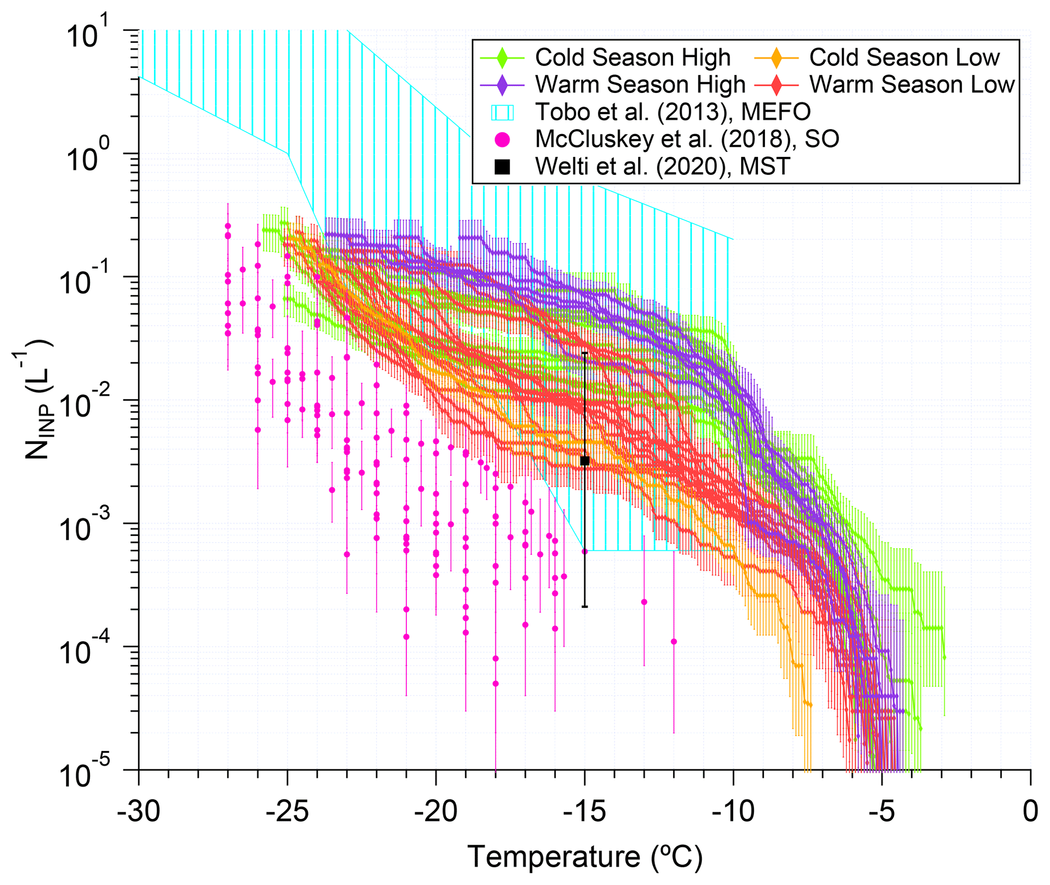
Figure 1 Cumulative N_INP as a function of temperature shown as green (cold season high), orange (cold season low), purple (warm season high), and red (warm season low) lines, respectively. Error bars show 95 % confidence intervals. The N_INP measured at the Manitou Experimental Forest Observatory (MEFO; Tobo et al., 2013), the Southern Ocean (SO; McCluskey et al., 2018a), and in the maritime South Temperate Zone (MST; only one value at −15 ^∘C, Welti et al., 2020) are shown as cyan background, magenta dots, and a black square, respectively. Error bars in McCluskey et al. (2018a) show 95 % confidence intervals. Error bars in Welti et al. (2020) show 80 % of the observations (excluding 10 % of highest and lowest values).

3 Results and Discussion

3.1 Temperature spectra of N_INP and its temporal variation

The temperature spectra of N_INP (i.e., N_INP as a function of temperature) are shown in Fig. 1. All filters had INPs that activated at −7.4 ^∘C, and within the detection limit, the warmest onset freezing temperature was −3 ^∘C. The curves of N_INP generally span a broad concentration range at any temperature, and below −10 ^∘C they do not intersect much. From −5 ^∘C to roughly −11 ^∘C, some N_INP spectra increased faster than others. Generally, however, all spectra have temperature ranges in which N_INP increases strongly and others in which there is a much flatter increase. Sharp increases in N_INP spectra may point to the presence of comparably high concentrations (“comparably high” at that temperature) of one or only a few types of INPs which all have similar features causing the ice activity (e.g., the same type of ice active protein expressed by bacteria or fungi as in Knackstedt et al., 2018). Flatter regions in N_INP spectra show up in temperature ranges in which only comparably few additional INPs become ice active with lowering temperature.

We classified samples into groups, discriminating them by concentration, depending on N_INP at −11 ^∘C to be either above or below $\mathrm{5}\times {\mathrm{10}}^{-\mathrm{3}}$ L⁻¹. Additionally, samples collected from May to September were assigned to the cold season, and those collected from October to March to the warm season. Based on this, the samples were classified into four clusters, i.e., cold season with high N_INP (CH) and low N_INP (CL), and warm season with high N_INP (WH) and low N_INP (WL), shown in different colors in Fig. 1. During the cold season, all samples were classified as belonging to the CH cluster, except for sample 11, which had been sampled from 14 to 22 August. During the warm season, N_INP spectra show a broader distribution. Five samples were attributed to the WH cluster, and 13 samples to the WL cluster. It is worth noting here, that comparably high N_INP spectra were observed throughout the year and no indication for a seasonal variation was found.

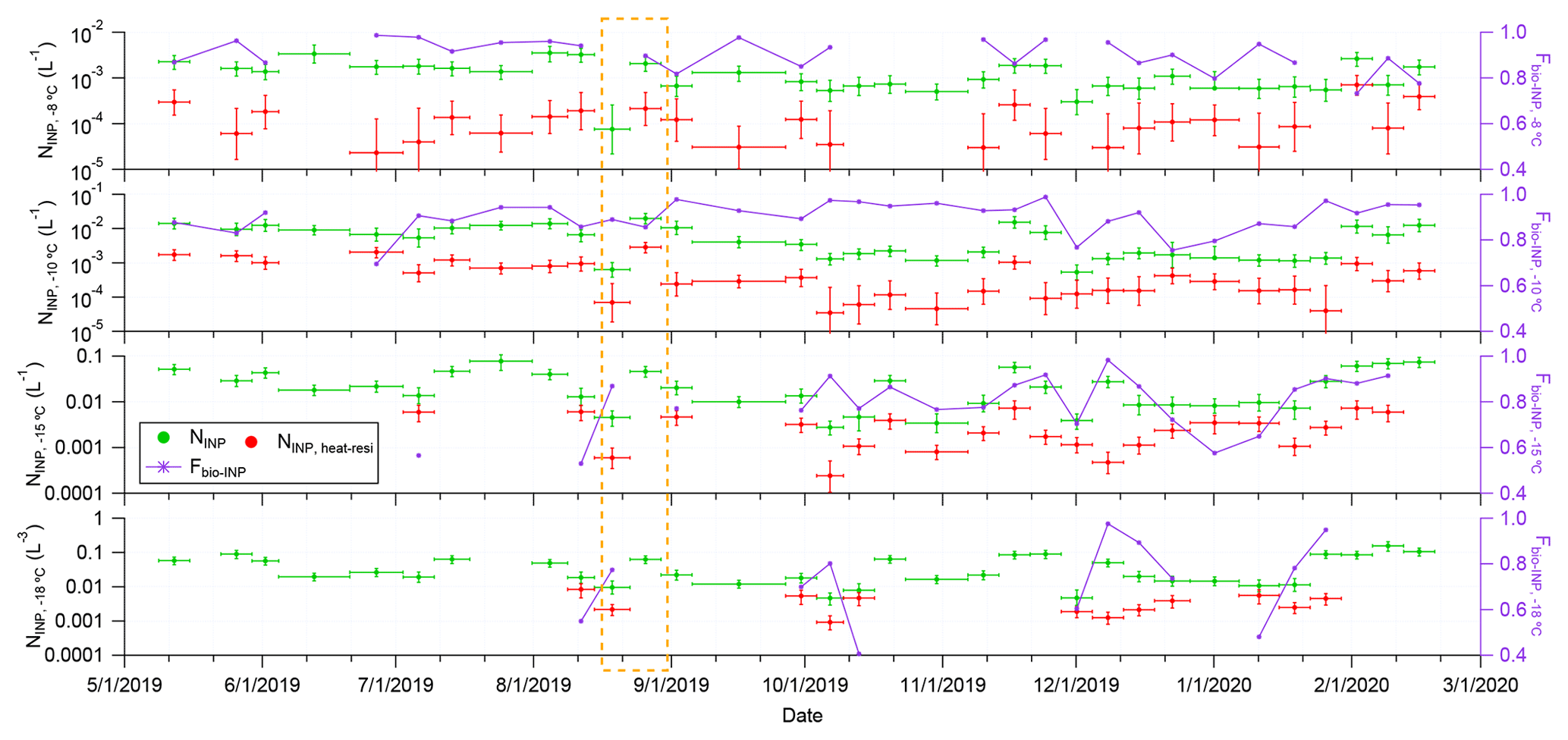
Figure 2 Time series of N_INP (green dots) and heat-resistant N_INP (N_{INP, heat_resi}, red dots) at −8, −10, −15, −18 ^∘C (from top to bottom). The fraction of bio-INP is shown as a purple line. The orange box highlights samples 11 and 12, i.e., the two samples used for a case study (discussed in Sect. 3.4).

The increase rate of N_INP (i.e., $\frac{\mathrm{d}{\log }_{\mathrm{10}}{N}_{\text{INP}}}{\mathrm{d}T}$) as a function of temperature is shown in Fig. S5, compiled from all curves shown in Fig. 1. A sharp increase in this parameter can be seen from −10 to −3 ^∘C. At −10 ^∘C, N_INP of most samples is already above 10⁻³ L⁻¹. For further characterizing of the N_INP spectra, the correlation coefficient of N_INP between different temperatures is shown in Fig. S6. A strong positive correlation of N_INP in the spectra at temperatures above −10 ^∘C was observed. The sharp increase in $\frac{\mathrm{d}{\log }_{\mathrm{10}}{N}_{\text{INP}}}{\mathrm{d}T}$ and the positive correlation at temperatures above −10 ^∘C points toward one type of INP being present in almost all samples in comparably high amounts, which again suggests a strong and rather more local source for these INPs.

Below −10 ^∘C, comparably low values and only small variations in $\frac{\mathrm{d}{\log }_{\mathrm{10}}{N}_{\text{INP}}}{\mathrm{d}T}$ are seen in Fig. S5, with a minimum from roughly −19 to −13 ^∘C. This temperature region can be attributed to one in which only comparably few INPs (from a broad range of different INP types from different sources) get ice active. The curves of N_INP below −10 ^∘C do not intersect much, which is also reflected by a strong positive correlation of N_INP in the spectra at temperatures below −10 ^∘C, shown in Fig. S6. However, it can also be seen in Fig. S6, that N_INP spectra at temperatures above and below −10 ^∘C exhibited a poor correlation with each other. This suggests that INPs which are ice active in these two temperature ranges are likely of different nature and origins.

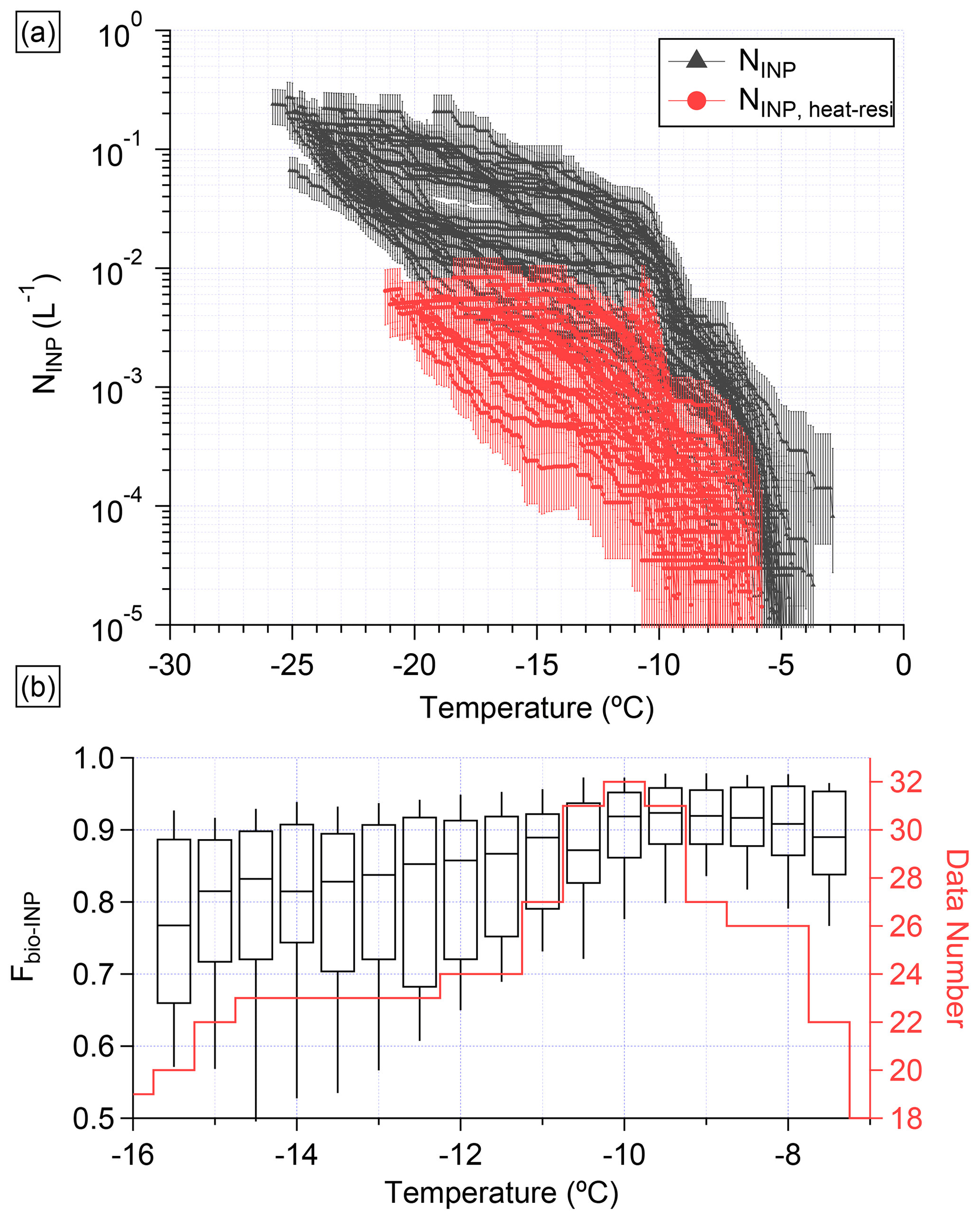
Figure 3 (a) Values for N_INP and N_{INP, heat_resi} as functions of temperature in black triangles and red dots, respectively. (b) Boxplot of F_bio-INP as a function of temperature. The red line shows how many different samples contributed to the boxplot at different temperatures (relating to the right axis).

Except for the N_INP spectra, distributions of all obtained N_INP were also examined separately at −8, −10, −15, and −18 ^∘C (see Fig. S7). Specifically, the skewness of the distribution of log ₁₀(N_INP) was determined, resulting in values of −0.9, −0.2, −0.24, and −0.1 at these four temperatures, respectively. This indicates that these distributions get closer to a lognormal distribution with lowering temperatures. Lognormal distributions are expected for parameters that went through a series of random dilutions (Ott, 1990), and they are typically observed for atmospheric distributions some distance away from sources. Therefore, INPs that are ice active at lower temperatures probably originated from long-range transport, while a more local source can be assumed at least for the INPs that are active at the higher temperatures (Welti et al., 2018).

Results from previous studies on INPs, added to Fig. 1, are compared with ours in the following discussion. Tobo et al. (2013) presented primary biological aerosol particles as an important source of INPs in a midlatitude ponderosa pine forest system (Manitou Experimental Forest Observatory, MEFO) in the summertime and the measured N_INP (cyan background in Fig. 1) in MEFO were slightly higher than ours. Note that the land cover and atmospheric environment in the MEFO site and in Punta Arenas are not comparable. Nevertheless, we here included Tobo et al. (2013) as one of their derived INP parameterizations. This will be discussed in Sect. 3.3. McCluskey et al. (2018a) found that the Southern Ocean has an incredibly pristine marine boundary layer with extremely low N_INP (see magenta dots in Fig. 1). The N_INP in this study is roughly more than 1 order of magnitude higher than that discussed in McCluskey et al. (2018a). Welti et al. (2020) summarized ship-based INP measurements from over the world and grouped the data into different climate zones. Here we compared N_INP with that in the Maritime South Temperate (MST) Zone and found that N_INP in this study is generally higher than the mean value in Welti et al. (2020).

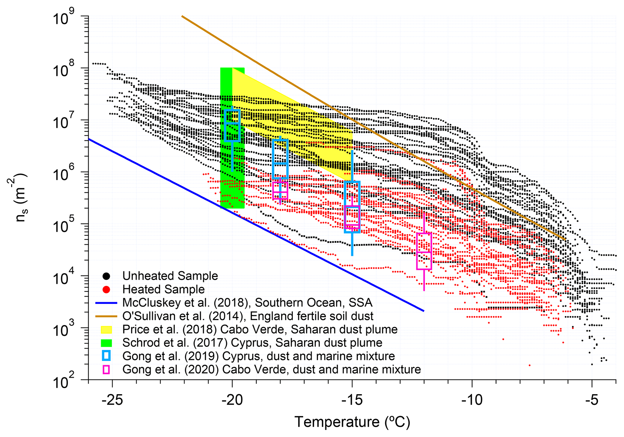
Figure 4 Ice active surface site density (n_s) of particles larger than 500 nm in diameter as a function of temperature for unheated and heated samples in black and red, respectively. Parameterizations from literature of n_s for marine aerosol from the Southern Ocean (SSA) and for English fertile soil dust are shown as blue and brown lines, respectively. Ranges of n_s for the Saharan dust plumes are shown as green and yellow areas. Ranges of n_s for ground-based data in marine regions influenced by Saharan dust are shown as blue and magenta box-plots. Respective literature is cited in the legend and in the main text. Data for Schrod et al. (2017), Gong et al. (2019), and Gong et al. (2020) are related to particle surface area >500 nm. Data for Price et al. (2018), O’Sullivan et al. (2018), and McCluskey et al. (2018a) are related to particle surface area >100 nm.

From additional atmospheric studies (not depicted in Fig. 1) it can be seen that continental aerosols generally have higher N_INP compared to marine aerosols. For example, concentrations of INP found for Saharan desert dust aerosols (Price et al., 2018), for biological particles from a forest (Tobo et al., 2013) or farmland (O’Sullivan et al., 2018), and for anthropogenic aerosols in the megacity of Beijing (Chen et al., 2018) were usually higher than those from marine aerosol particles (DeMott et al., 2016; McCluskey et al., 2018a). Gong et al. (2020) examined INPs from the ocean, the ambient environment, and from cloud water at the Cabo Verde islands, and found that marine aerosols from sea spray production only explained a very minor fraction of N_INP in the atmosphere and in cloud water. Tatzelt et al. (2021), who collected data in the Southern Ocean and Welti et al. (2020), who examined a broader, more global dataset, found that the ship-based measurements of ambient N_INP show 1–2 orders of magnitude lower mean concentrations for clean marine conditions than for continental observations. Therefore, INPs in our study most likely originated from land and more evidence for this is discussed in the following sections.

3.2 Contribution of biogenic INPs

We examined the nature of the observed INPs further. It is typically inferred that INPs that are sensitive to heat are protein-based biogenic INPs, i.e., INPs of biological origin (Christner et al., 2008). We refer to those as bio-INPs in the following discussion. As mentioned above, in this study the particle suspensions were heated to 95 ^∘C for 1 h to destroy the ice activity of bio-INPs. The sample was then examined in INDA to obtain N_INP for heat-resistant INPs (N_{INP, heat_resi}). Figure 2 shows the time series of N_INP for untreated samples as green dots, together with N_{INP, heat_resi} as red dots, determined at temperatures of −8, −10, −15, and −18 ^∘C. The N_INP varied by roughly 1–2 orders of magnitude at each temperature. However, as discussed above, a seasonal cycle does not become obvious, but N_{INP, heat_resi} is clearly always lower than N_INP. Therefore, Fig. 2 also shows fractions of bio-INP (F_bio-INP), calculated as

$$\begin{array}{}\text{(6)}& F_{\text{bio-INP}}={\displaystyle \frac{N_{\text{INP}}-N_{\text{INP, heat\_resi}}}{N_{\text{INP}}}}.\end{array}$$

Figure 5 Scatter plot of measured N_INP against predicted N_INP obtained from parameterizations by (a) DeMott et al. (2010) and (b) Tobo et al. (2013).

At −8 and −10 ^∘C, F_bio-INP was generally above 80 %. For the lower temperatures displayed in Fig. 2, all wells of the PCR trays were already frozen for a number of samples (see Fig. S3). The detection limit of INDA depends on experimental parameters such as the droplet volume and the volume of air that contributed INPs to each droplet. In this study, the upper measurement limit of INDA is roughly 10⁻² L⁻¹. Therefore, and since no LINA measurements had been done for the heated samples, values for N_{INP, heat_resi} and F_bio-INP are not available for all samples.

In Fig. 3a, N_INP spectra for untreated and heated samples are shown together as black and red lines, respectively. It again becomes obvious that heating lowered the observed ice activity. Figure 3b shows boxplots of F_bio-INP as a function of temperature. The red line shows how many different samples contributed at different temperatures, and data are only shown for cases when more than half of all samples contributed. It is clear that above −10 ^∘C, more than 90 % (median value) of all INPs were of proteinaceous biogenic origin. From −10 ^∘C to lower temperatures, a decreasing trend in F_bio-INP was observed with decreasing temperature. This observation is in line with O’Sullivan et al. (2018) and Testa et al. (2021), who also found a contribution of bio-INPs which was getting lower as temperatures decreased. In our study, at −16 ^∘C generally more than 70 % of all INPs are still bio-INPs, which is comparable to values reported by previous studies conducted in agricultural regions (Garcia et al., 2012; Suski et al., 2018; O’Sullivan et al., 2018; Testa et al., 2021).

All of this points towards a strong contribution of bio-INPs to the observed aerosol, and to INPs originating most likely from sources which would not be too far away and likely terrestrial. The region of the Southern Ocean is known for high fractions of supercooled liquid clouds (Choi et al., 2010), which are thought to originate from a lack of INPs connected to fewer terrestrial sources in the Southern Hemisphere (Zhang et al., 2018). While low N_INP were observed in the open ocean (McCluskey et al., 2018a; Welti et al., 2020; Tatzelt et al., 2021), we observed N_INP that are more comparable to continental sites. When examining satellite observations given in Choi et al. (2010) more closely, it can be seen that the effect of high fractions of supercooled liquid clouds is less pronounced close to South America. This, together with our observations, implies that air masses, at least those at lower altitudes, will quickly be enriched in INPs when coming into contact with continental or more generally terrestrial sources. A similar observation was also made by Tatzelt et al. (2021) based on observations performed in the frame of a circumvention of Antarctica.

3.3 INP surface site density and correlation with particle number concentration

Particle number concentration for the size range above 500 nm (N_>500 nm) (DeMott et al., 2010) or ice active surface site density (n_s) (DeMott, 1995; Connolly et al., 2009; Niemand et al., 2012) are widely used to quantify the heterogeneous ice nucleation activity. Current models (Steinke et al., 2021) and remote-sensing studies (Mamouri and Ansmann, 2015) predict N_INP based on either N_>500 nm or on n_s. Therefore, a precise understanding of n_s and the relation between N_>500 nm and N_INP in different environments is highly needed.

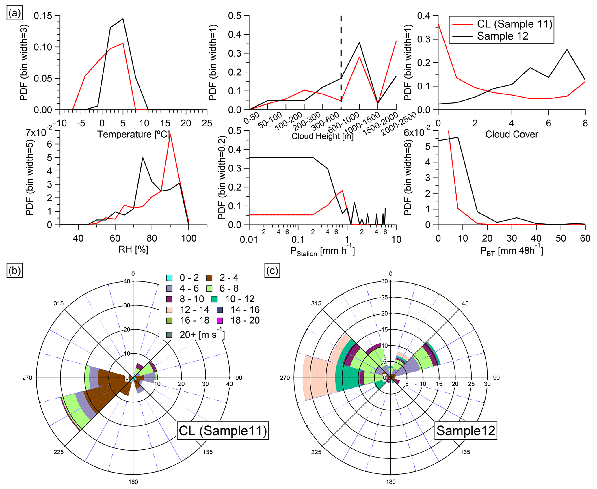
Figure 6 (a) Probability density function (PDF) of temperature, cloud height, cloud cover, relative humidity (RH), precipitation measured at the station (P_Station), and cumulative precipitation along the backward trajectory in the past 2 d (P_BT) during samples 11 (red) and 12 (black). The dashed line in the cloud height panel shows the measurement station height. (b) The wind rose plot during sample 11. (c) The wind rose plot during sample 12.

Some previous studies found that the majority of INPs were supermicron in size (Mason et al., 2016; Creamean et al., 2018; Gong et al., 2020). Therefore, we derived n_s in two different ways: (i) using the total particle surface area and (ii) using the particle surface area for particles with sizes >500 nm. The latter surface areas were, however, roughly only about 30 % lower than the former, as the majority of the particle surface area was contributed by larger particles. In Fig. 4, n_s based on particle surface area for particles with sizes >500 nm is shown, but the following discussion is generally the same for both datasets.

Figure 4 shows n_s of unheated samples as a function of temperature in black dots. Assuming the heating process only destroys the structure of proteins but does not change the total particle surface area of an aerosol noticeably, we can also calculate n_s of heated samples, shown as red dots in Fig. 4. The scatter in n_s is large for both unheated and heated samples, independent of the use of the total particle surface area or only that for particles >500 nm. However, such a spread is not unusual for atmospheric data, of which we show some for a comparison to literature data in Fig. 4 as well. These literature data include a parameterization of n_s for marine aerosol obtained from measurements in the Southern Ocean (McCluskey et al., 2018b). Due to the remote location at which these data were obtained, INPs likely all originated from sea spray aerosol (SSA). Also shown is a parameterization derived for English fertile soil dust (O'Sullivan et al., 2014), together with data of Saharan dust plumes from airborne measurements (Schrod et al., 2017; Price et al., 2018) and from ground-based data in marine regions influenced by Saharan dust (Cyprus and Cabo Verde, Gong et al., 2019, 2020, respectively). Although we are aware of the fact that a previous study (Testa et al., 2021) found that Argentinian soil dust contains illite and a small fraction of K-feldspar, and that these mineral dusts may also contribute INPs observed in our study, we refrain from comparing with n_s parameterizations obtained from respective laboratory studies (such as Hiranuma et al. (2015) for illite NX or Harrison et al. (2019) for K-feldspar), as these relate n_s purely to the surface area of these minerals, a parameter which is not available for our atmospheric data.

Regarding Fig. 4, it is clear that at all temperatures, n_s of our unheated samples is higher than that of the Southern Ocean's SSA (McCluskey et al., 2018b) by up to several orders of magnitude, indicating that the aerosol we examined in southern Chile in total is more ice active per surface area than SSA from remote regions in the Southern Ocean, i.e., the ocean surrounding southern Chile. For the English fertile soil dust (O'Sullivan et al., 2014) above about −15 ^∘C, n_s is roughly in the midst of our unheated data. Concerning heated data, O'Sullivan et al. (2014) found n_s of heated samples to be reduced by 1–2 orders of magnitude, also similar to our results (data not shown as no parameterization was given). These comparisons again suggest that INPs at our sampling site were influenced by terrestrial biogenic soil dust sources.

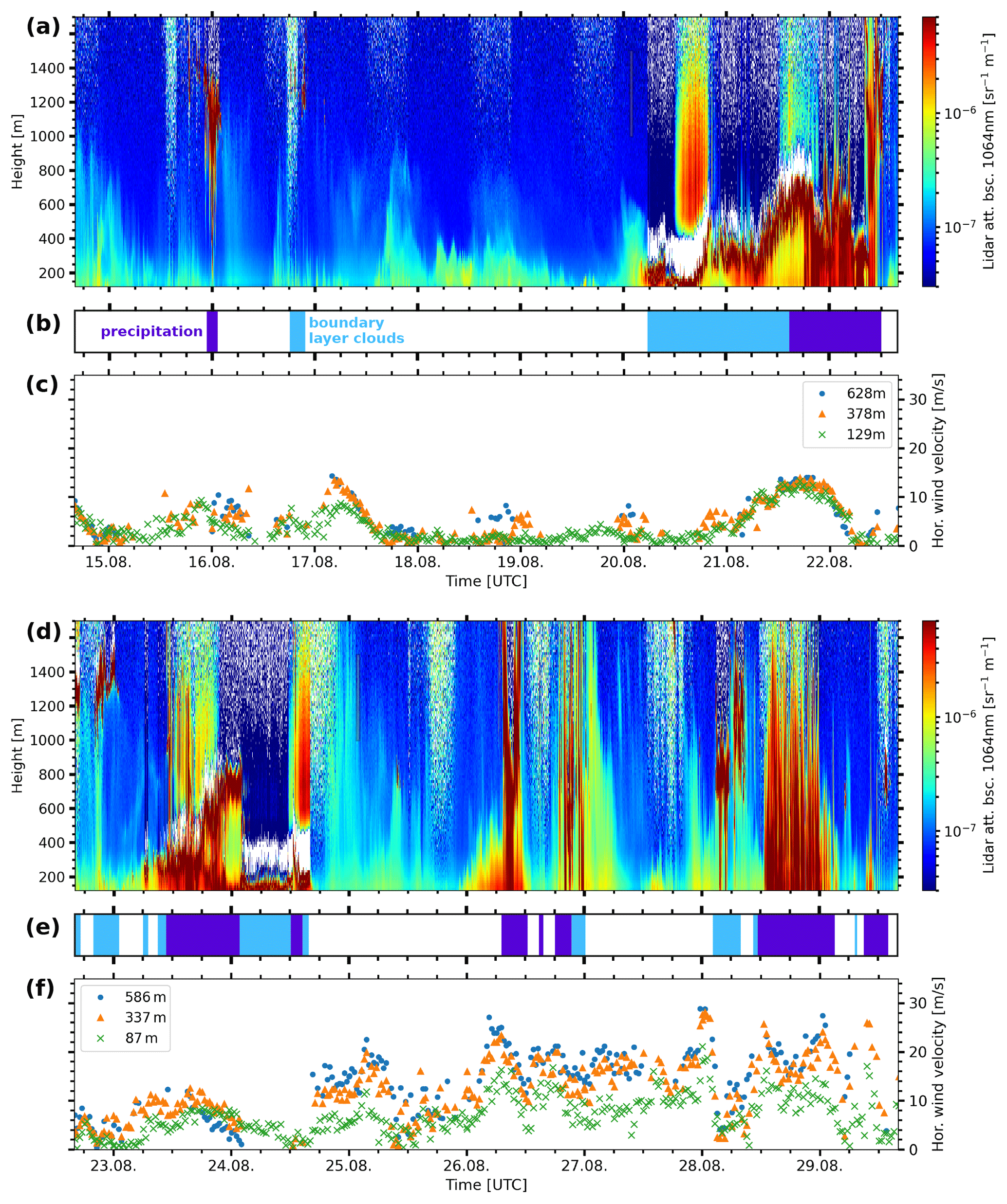
Figure 7 Overview of aerosol and cloud conditions at Punta Arenas during which sample 11 and 12 were collected. (a, d) Time-height cross-section of attenuated backscatter at 1064 nm at 30 s temporal and 14.9 m vertical resolution obtained from the ceilometer. (b, e) Periods of boundary layer clouds and precipitation derived from the Cloudnet target classification. (c, f) Horizontal wind velocity retrieved from the Doppler lidar scans at heights of 129, 378, and 62 m.

Values for n_s from ground-based measurements in marine regions influenced by Saharan dust (Cyprus and Cabo Verde, Gong et al., 2019, 2020, respectively) are shown in Fig. 4, where, however, those values were adjusted such that they also relate to the surface area for particles with sizes >500 nm. These n_s values are above those for SSA, likely due to long-range transport of Saharan dust to both Cyprus and Cabo Verde. Agreement with our data can be seen for heated samples, representing the non-biogenic INPs, at higher temperatures and for untreated samples only at −20 ^∘C. At sampling sites of both Cyprus and Cabo Verde, influence from local landmasses were minimized by sampling air at the coast and upwind of the islands, different from the sampling site used for the data which we presented here. Overall, this is again one more indication that data in the presented study were influenced by additional sources of very ice active INP.

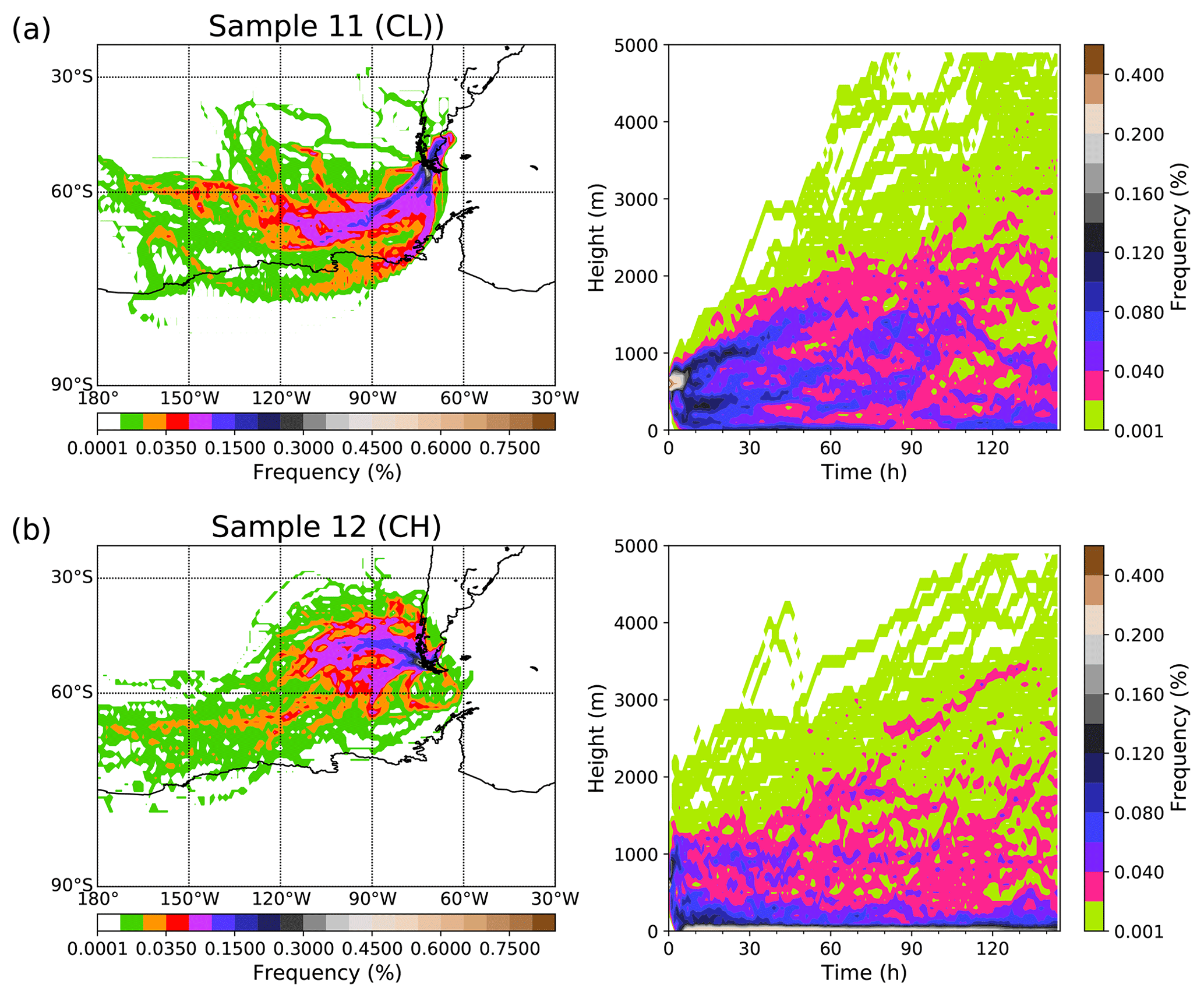
Figure 8 Relative frequency of backward trajectories ending at the Cerro Mirador site (600 m a.s.l.) with 1 h resolution, based on a 1^∘ by 1^∘ grid size (a, b) and the corresponding relative frequency of backward trajectory height (c, d) during sample 11 (a) and sample 12 (b).

A comparison with n_s from Saharan dust plumes is only possible at −20 ^∘C for Schrod et al. (2017) or below −15 ^∘C for Price et al. (2018). The range of values reported by Schrod et al. (2017) covers the range in which all of our unheated and heated data can be found. On the other hand, data from Price et al. (2018) are at the upper half of data we obtained for unheated samples, but clearly above the heated samples. Both sets of literature data are mostly much higher than our heated data, which we assumed to be representative of a non-biogenic, dust-dominated aerosol. These higher values may originate from a higher fraction of particles and total particle surface area being contributed by dust particles in the Saharan dust plumes. On the other hand, data in both Schrod et al. (2017) and Price et al. (2018) may have been influenced by biogenic contributions to the INPs, since Kleber et al. (2007) already found that protein complexes can be well preserved and possibly even accumulated when connected to mineral dust surfaces. Overall, the variability of n_s for atmospheric samples, both on a local scale but also between different locations, becomes obvious by the comparison which we presented here.

Next, two further INP parameterizations are evaluated. Figure 5 shows the measured N_INP against predicted N_INP based on parameterizations by DeMott et al. (2010) and Tobo et al. (2013) in panels (a) and (b), respectively. DeMott et al. (2010) summarized 9 field studies at different locations over the world, realized over 14 years, and proposed a fitting function to predict global average N_INP. This parameterization excluded SSA-dominated environments. It is clear that this parameterization overestimates N_INP observed in our study by 1–2 orders of magnitude. Tobo et al. (2013) proposed a parameterization, based on measurements in a forest ecosystem, to predict biogenic N_INP. The predicted N_INP is often comparable to our measured N_INP, with roughly 50 % of the predicted N_INP being within a factor of 2 of the measured values.

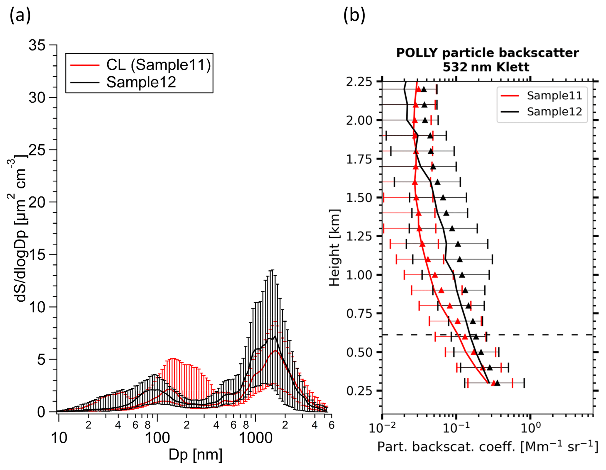
Figure 9 (a) Particle surface area size distribution for samples 11 (red) and 12 (black). (b) Vertical profile of particle backscatter coefficient during samples 11 (red) and 12 (black). The triangles show the mean values, and the dashed line shows the height of the Cerro Mirador station. The solid lines in both panels show the median value, and error bars show the 25th to 75th percentile.

From the above comparisons between different data and parameterizations, it can be seen that there is a large variability in INPs in both their concentrations and their ice activity expressed e.g., as ice active surface site density. This is rooted in the fact that many different types of particles across the range from mineral dusts to microorganisms show ice activity, and that atmospheric INPs therefore originate in a multitude of different sources which have changing source strengths in both space and time. Therefore, at least the aerosol types prevailing in the area have to be considered when choosing a parameterization to describe atmospheric INPs. Additionally, in the case examined in this study, there are several indications, as discussed above, that INPs in the examined aerosol, particularly those ice active INPs at higher temperatures, are dominated by a strong biogenic terrestrial source present in the surrounding area.

3.4 Case Study

We performed a case study to assess the influence of meteorology and aerosol sources on INP concentrations. As mentioned in Sect. 3.1, samples collected in the cold season have high N_INP, except for sample 11 that was sampled from 14 to 22 August 2019. Here we compare several meteorological and aerosol-related parameters for sample 11 and sample 12, the latter sampled from 22 to 29 August 2019. Figure 6a shows the probability density functions (PDFs) of temperature, cloud height, cloud cover, relative humidity (RH), precipitation in the station (P_Station), and the cumulative precipitation along the backward trajectory in the past 2 d (P_BT) during sample 11 (in red) and sample 12 (in black). Backward trajectory analyses were performed with the HYbrid Single-Particle Lagrangian Integrated Trajectory (HYSPLIT) model (Stein et al., 2015), based on the Global Data Assimilation System (GDAS) meteorological data.

Surface temperatures, which were taken from a station at the Punta Arenas airport, were slightly lower during the period of sample 11 (Fig. 6a). In terms of cloud cover, given as okta values following Jones (1992), the station observations (see Fig. 6a) and the remote-sensing observations (see Fig. 7a, d) both show a significantly higher cloud cover during the sampling period of sample 12. A long period with a cloud-free boundary layer during sample 11 is an especially striking feature, which coincides with high surface pressure values, indicative of calm weather conditions.

Figure 10 (a) Probability density function (PDF) of temperature, relative humidity (RH), cloud cover, cloud height, precipitation measured at the station (P_Station), and cumulative precipitation along the backward trajectory in the past 2 d (P_BT) averaged for all samples collected during cold season high (CH, blue lines), warm season high (WH, green lines), and warm season low (WL, magenta lines). (b, c, d) The wind rose plots for CH, WH, and WL.

Precipitation was more frequent and more intense during sample 12 compared to the week before, which can be seen from PDFs of P_Station and P_BT in Fig. 6a, and time series of precipitation derived from the Cloudnet target classification in Fig. 7b and e. When rain occurs, particles can be washed out due to impaction, turbulent and Brownian diffusion as well as phoretic phenomena, or simply because they acted as cloud condensation nuclei (CCN) during cloud formation. These processes depend on the size, chemical composition, and concentration of particles (Pruppacher et al., 1998; Chate et al., 2011). However, raindrops can disperse soil bacteria and other bio-aerosols into ambient air (Joung et al., 2017). Furthermore, rain impaction on plants might contribute to aerosolization of biogenic INPs (Huffman et al., 2013; Prenni et al., 2013; Tobo et al., 2013; Testa et al., 2021). The RH is also known as a factor affecting the INP population in a number of ways (Huffman et al., 2013; Testa et al., 2021). Testa et al. (2021) found that N_INP at −12 ^∘C is positively correlated with RH, but N_INP at lower temperatures ($<-\mathrm{20}$ ^∘C) is negatively correlated with RH. In this study, we found that RH is somewhat higher for sample 11 while N_INP at $>-\mathrm{20}$ ^∘C is lower than in sample 12.

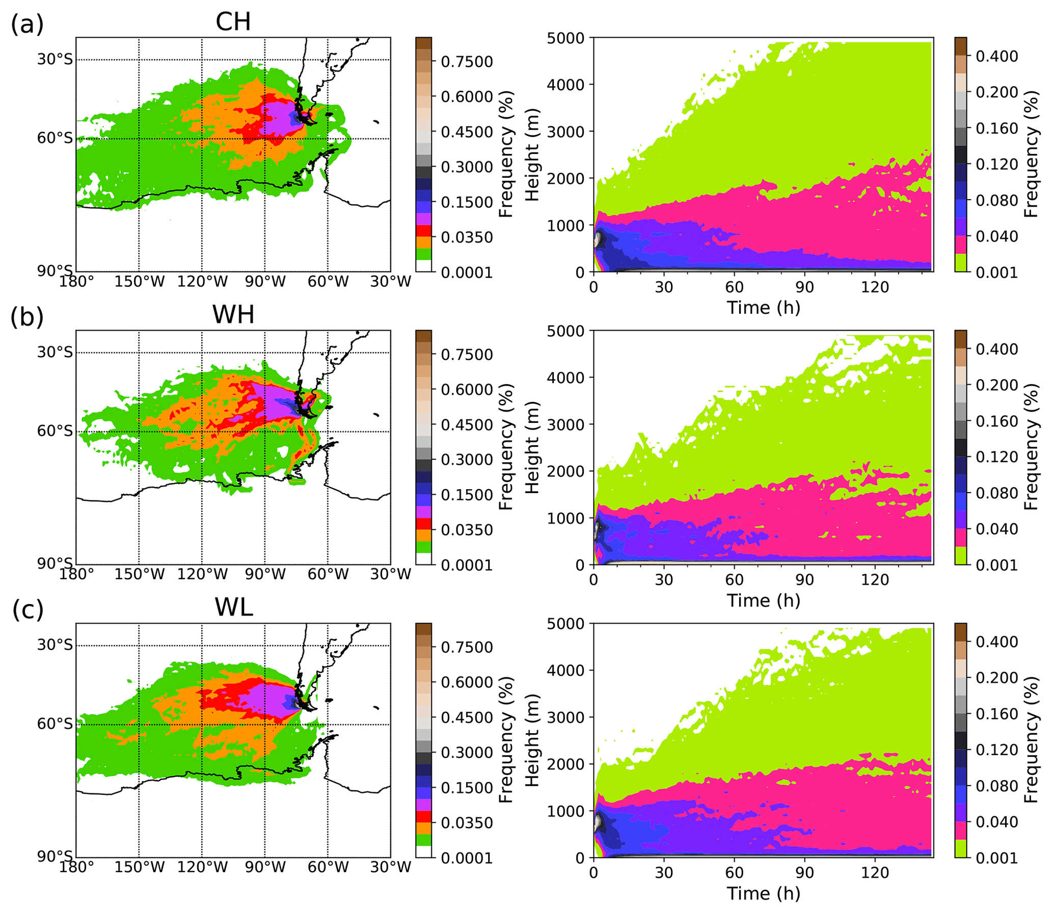
Figure 11 Relative frequency of backward trajectories ending at Cerro Mirador site (600 m a.s.l.) with 1 h resolution, based on a 1^∘ by 1^∘ grid size (left) and the corresponding relative frequency of backward trajectory height (right) during cold season high (CH, a), warm season high (WH, b), and warm season low (WL, c).

During the collection time of sample 11, low wind speeds <10 m s⁻¹ prevailed and the wind most often came from a southwestern direction (Figs. 6b and 7c). Boundary-layer wind shear, as it can be inferred from the difference of the wind values at the three different height levels, was also low, indicating only weak turbulent conditions. The frequency of backward trajectories in sample 11 (Fig. 8a) is in good agreement with the histogram of wind directions. In sample 12, the wind direction was mostly from the west with a stronger wind speed (Figs. 6c and 7f). Compared to sample 11, the wind shear is higher as well (Fig. 7f). The frequency of backward trajectories in sample 12 (Fig. 8b) shows that air parcels traveled from the west to the measurement station. Considering the local geography, air parcels collected for both samples covered roughly the same distance over mountainous land, interspersed with fjords, in advance to arrival at the sampling site.

The measurement station was exposed to free-tropospheric conditions for different amounts of time during the 2 examined weeks. Typically, the boundary-layer top is associated with a notable decrease of particle backscatter (Baars et al., 2008). As becomes evident from Fig. 7a, the boundary layer heights for sample 11 showed a strong diurnal cycle with daytime maxima around 1100 m height and nighttime minima of 500 m or below. Thus, the top of Cerro Mirador was influenced by the free troposphere for a significant fraction of the sampling period. During sample 12, the boundary-layer tops were significantly higher, peaking at 1900 m during daytime, while nighttime lows were rarely below 700 m, leading to the sampling of mostly boundary layer air. This difference in air mass origin can also be seen in the right panels of Fig. 8, clearly showing that collected air masses spent a higher fraction of time in the free troposphere for sample 11.

Figure 12 (a) Particle surface area size distribution for cold season high (CH, blue), warm season high (WH, green), and warm season low (WL, magenta). (b) Vertical profile of particle backscatter coefficient during CH, WH, and WL. The triangles show the mean values, and the dashed lines show the height of the Cerro Mirador station. The solid lines in both panels show the median value, and the error bars show the 25th to 75th percentile.

Figure 9 shows the particle surface area size distribution (PSSD) and the vertical profiles of particle backscatter coefficients for samples 11 (red line) and 12 (black line). The PSSDs are bimodal with a minimum around 300 nm. The concentration of the larger mode is slightly higher in sample 12 than in sample 11. Furthermore, the particle backscatter coefficient is higher throughout the boundary layer depth and above, indicating a generally higher aerosol load observed for sample 12.

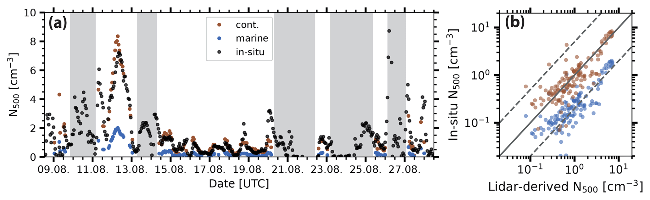
Figure 13 (a) Time series (during sample 10, 11, and 12) of in situ measured N_>500 nm in black dots, and lidar-retrieved N_>500 nm when assuming a lidar ratio typical for marine or continental particles in blue and brown dots, respectively. The periods without lidar profiles are marked in gray. (b) The in situ measured N_>500 nm against the lidar-retrieved N_>500 nm when assuming a lidar ratio typical for marine or continental particles (during sample 10, 11, and 12) in blue and brown dots, respectively.

In summary, the examination of meteorological conditions and aerosol features of the two subsequent samples from the cold season with strongly contrasting N_INP (low for sample 11, high or sample 12), yielded differences. For sample 12, simultaneously with high N_INP higher wind speeds prevailed, precipitation was more frequent, and concentrations of large particles (>500 nm) were slightly enhanced. Generally, higher aerosol concentrations are evident throughout the boundary layer, as indicated by higher particle backscatter coefficients. As discussed above, it is known that rain events can lead to more bio-aerosols, including soil bacteria, being ejected into ambient air, some of which may be INPs. Higher N_INP may have been caused by the addition of soil dust or biogenic particles over land to the sampled air masses. However, as the comparison of only two samples is of limited value, an additional discussion concerning processes which may control N_INP are given in the following section.

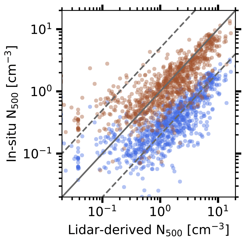
Figure 14 In situ measured N_>500 nm against the lidar-retrieved N_>500 nm when assuming a lidar-ratio typical for marine or continental particles (including data available from May 2019 to March 2020) in blue and brown dots, respectively.

3.5 Processes controlling N_INP

To obtain additional insights into processes controlling the INP population, we studied the parameters that were examined for the case study in the previous section for all samples as well. For that, samples were classified into four clusters, i.e., WH, WL, CH, and CL, based on N_INP, as described in Sect. 3.1.

As data for the only case attributed to CL were already shown in the previous section, Figs. 10, 11 and 12 show averaged results for WH, WL, and CH only. Some generally expected differences between warm and cold seasons become obvious. Both warm season clusters had similar higher temperatures and similar lower RH than both cold season clusters (Fig. 10a). Similarly, both warm season clusters had similar bi-modal PSSD, with particle number and surface area concentrations being ∼2 times higher than for both winter clusters (Fig. 12a). They also had similar but higher values of particle backscatter coefficients at all heights, visible in the vertical profiles shown in Fig. 12b. The similarity in particle abundance for both WH and WL shows that parameters related to particle abundance alone cannot predict INP concentrations well for the data which we presented here.

Similar cloud heights were observed for all clusters, with clouds at roughly 600 to 1500 m. The overall cloud cover during WH, WL, and CH was comparable (Fig. 10a) but higher than during CL (Fig. 6a). Similarly, the wind rose plots show that wind speeds during WH, WL, and CH were comparable (Fig. 10b), but higher than during CL (Fig. 6b). While 37 % of the time the observed wind speeds during CL were below 4 m s⁻¹, less than 15 % were as low during CH. During the warm season, such low wind speeds were never observed. The wind direction during WH, WL, and CH were mainly from the west, but wind directions during CL were mainly from the southwest. As for the case study, also for all clusters the backward trajectory frequencies shown in Fig. 11 (left panel) are in good agreement with wind directions shown in the wind rose plots. During WH, WL, and CH, the air parcels featured similar paths, mainly originating from the Southern Ocean to the west of the sampling location at Cerro Mirador. The vast majority of trajectories stayed north of 65^∘ S for these three clusters, while more than 20 % of trajectories during CL passed much further south. Also, there is no pronounced difference in the time air masses spent in the boundary layer during WH, WL, and CH (Fig. 11 right panel). None of these parameters related to clouds, wind speed or direction gives clear insights into why WH and WL featured such clearly different N_INP.

Based on lidar data, further agreement for WH, WL, and CH was seen. With the exception of sample 11, no extended periods of boundary-layer top heights below 800 m were observed. Furthermore, mineral dust in the free troposphere was not observed during the sampling period (Radenz et al., 2021). This and the origin of the backward trajectories discussed above make it unlikely that observed high concentrations of INPs originated from mineral dust particles.

Finally, P_Station and P_BT during WH and CH were higher than during WL and CL. Among the parameters discussed above, precipitation was the only one that distinguished high from low N_INP. As mentioned before, raindrops can disperse soil bacteria and other bio-aerosols into ambient air. Rain impaction on plants might also contribute to biological INPs. We suggest that precipitation was indeed an important meteorological parameter affecting INP concentrations in this study.

In summary, we found that the meteorological parameters, including cloud height, cloud cover, and RH are not directly related to N_INP. Instead, we suggest that strong precipitation is one of the most important parameters to enhance the N_INP in both cold and warm seasons. The air masses mainly come from the Southern Ocean, without differences during cold and warm seasons. The particle surface area concentration in the cold season is much lower than in the warm season. However, the N_INP during the cold season are all in the higher concentration cluster, except for one sample.

3.6 Relationship between in situ measured N_>500 nm and lidar data

In this section, N_>500 nm obtained from the in situ measurements is compared with values obtained from lidar data. The retrieval of the latter is based on the profiles of particle backscatter coefficients at 532 nm (Sect. 2.5). The extinction coefficient is then calculated using typical extinction to backscatter (lidar) ratios for marine (20 sr) and continental (50 sr) aerosols (Müller et al., 2007; Bohlmann et al., 2018). In our study, the optical properties were then taken for a height of 622 m above the remote-sensing site. The optical properties were converted to particle number concentrations with the conversion factors for marine and continental aerosol, respectively, as given by Mamouri and Ansmann (2016).

Figure 13a shows an exemplary time series (during sample 10, 11, and 12) of in situ measured (black dots) and lidar-retrieved (a lidar ratio typical for marine particles in blue dots and for continental particles in brown dots) N_>500 nm and (b) shows the corresponding scatter plot. It can be seen that values retrieved when assuming continental aerosol fit well with the in situ data, while assuming marine aerosol resulted in N_>500 nm that is clearly too low. Figure 14 shows the in situ measured N_>500 nm against the lidar-retrieved N_>500 nm when assuming a lidar ratio typical for marine or continental particles in blue and brown dots, respectively, including all data available from May 2019 to March 2020. A linear fit in the logarithmic space through the continental data shown in Fig. 14 yields an R- value of 0.72 with a slope of 0.99 and an intercept of 0.003. Therefore, we find that N_>500 nm derived from lidar data when assuming a lidar ratio typical for continental aerosol generally fits well with the colocated in situ data. As this retrieval was done for an altitude of 622 m, i.e., well elevated above the lidar location, it can be concluded from the comparison that the boundary layer was typically well mixed concerning large aerosol particles of continental origin. Generally, indeed, a well-mixed boundary layer was also seen during most of the observation periods, as the particle backscatter coefficients were often constant for altitudes between 250 m and 1.2 km (as also indicated in Fig. 3 of Radenz et al., 2021).

The lidar comparison suggested that the large aerosol particles (>500 nm) are of continental origin, which is consistent with the INP source analysis. Moreover, INP concentrations could generally be derived well based on in situ derived N_>500 nm values when using the parameterization from Tobo et al. (2013) (as discussed in Sect. 3.2). Together, these results suggest that, for this study in the region of Punta Arenas, N_INP valid throughout the boundary layer may generally be derived based on lidar data when assuming the presence of continental aerosol in the retrieval of N_>500 nm. However, more research, combining in situ and offline INP sampling with remote-sensing methods is needed before this claim can fully be made.

4 Conclusions and outlook

This study analyzed annual offline measurements of INP number concentrations (N_INP) that were performed in the framework of the Dynamics, Aerosol, Cloud, And Precipitation Observations in the Pristine Environment of the Southern Ocean (DACAPO-PESO) campaign at Cerro Mirador near Punta Arenas (Chile). Measurements of aerosol particle surface area size distribution, synergistic radar and lidar observations, backward trajectory calculations, and surface observations of meteorology (temperature, RH, cloud cover, cloud height, precipitation) were used to put obtained N_INP into context.

The highest ice nucleation temperature we observed was −3 ^∘C and all samples were activated at −7.4 ^∘C, where it should be mentioned that these values are instrument dependent. The INP spectra (N_INP as a function of temperature) showed a sharp increase of N_INP from this measurement onset down to $\sim -\mathrm{10}$ ^∘C. The N_INP in this study are much higher than that in the Southern Ocean (McCluskey et al., 2018a), but comparable with measurements in an agricultural area in Argentina (Testa et al., 2021) and a forestry environment in the US (Tobo et al., 2013). No clear seasonal variation was observed. At high temperatures ($>-\mathrm{10}$ ^∘C), roughly 90 % of all INPs were proteinaceous and hence of biogenic origin. This fraction lowered to ∼70 % between −10 and −16 ^∘C, indicating an important contribution of biogenic INPs all over this temperature range.

Ice active surface site density (n_s) in this study is much higher than for clean marine aerosol in the Southern Ocean, but similar to English fertile soil dust samples. Similar to observations reported for the latter, n_s for heated samples also decreased by 1–2 orders of magnitude, induced by the destruction of proteinaceous INPs by the heat treatment. Values for n_s for heat-treated samples are also closer to those for marine aerosols that are slightly influenced by mineral dust particles. The parameterization based on particle number concentrations in the size range larger than 500 nm (N_>500 nm) from DeMott et al. (2010), representing global N_INP in non-marine environments, overestimated measured N_INP by up to 2 orders of magnitude. However, the parameterization from Tobo et al. (2013), representing biological particles from a forestry environment, yields N_INP comparable to values obtained in this study.

Backward trajectories showed that air masses generally came from the Southern Ocean, mainly from west or southwest directions, passing at least 150 km of mountainous land, interspersed with fjords, between the ocean and the measurement site. The comparison between comparably high and low N_INP in both the cold and warm seasons pointed toward precipitation as the sole main meteorological parameter which may explain the observed variations in N_INP. Mobilization of INPs due to precipitation has been described before, and overall we suggest that high N_INP of biogenic INP originated from terrestrial sources and were added to the air masses during the overflow of land, before arriving at the measurement site. When assuming that aerosol particles are of continental origin, the lidar-retrieved N_>500 nm values fit well with the in situ N_>500 nm. This comparison also suggests that particles >500 nm were well mixed in the PBL. We conclude that for the presented dataset, N_INP in the PBL could be derived based on lidar-retrieved N_>500 nm and the INP parameterization in Tobo et al. (2013).

This study shows a significant land source of INPs at the tip of southern South America. Using a combination of meteorological data, backward trajectories and lidar analysis, this study provides insights into the mechanisms controlling the observed INPs. However, considering the complex nature and diverse aerosol sources, open questions remain. One interesting detail from our study is that the cold season shows generally lower particle number concentrations, but almost always high INP concentrations. Atmospheric INP concentrations, sources of INPs and processes controlling these parameters cannot solely be answered by one study, even if the study covered an annual dataset. Further studies are needed, also in this region. Such studies should include a chemical analysis of the aerosol to possibly aid a better understanding of INP sources. Additionally, a combination with measurements of biological particles may be helpful, or examinations of INPs in rainwater. Furthermore, a higher temporal resolution of INP measurements, together with additional parameters such as those used here, could help to gain more detailed insight into the nature and sources of INPs.