the Creative Commons Attribution 4.0 License.
the Creative Commons Attribution 4.0 License.
 | 29 Jun 2021
Tropospheric and stratospheric wildfire smoke profiling with lidar: mass, surface area, CCN, and INP retrieval
Kevin Ohneiser
Rodanthi-Elisavet Mamouri
Daniel A. Knopf
Igor Veselovskii
Holger Baars
Ronny Engelmann
Andreas Foth
Cristofer Jimenez
Patric Seifert
Boris Barja
We present retrievals of tropospheric and stratospheric height profiles of particle mass, volume, surface area, and number concentrations in the case of wildfire smoke layers as well as estimates of smoke-related cloud condensation nuclei (CCN) and ice-nucleating particle (INP) concentrations from backscatter lidar measurements on the ground and in space. Conversion factors used to convert the optical measurements into microphysical properties play a central role in the data analysis, in addition to estimates of the smoke extinction-to-backscatter ratios required to obtain smoke extinction coefficients. The set of needed conversion parameters for wildfire smoke is derived from AERONET observations of major smoke events, e.g., in western Canada in August 2017, California in September 2020, and southeastern Australia in January–February 2020 as well as from AERONET long-term observations of smoke in the Amazon region, southern Africa, and Southeast Asia. The new smoke analysis scheme is applied to CALIPSO observations of tropospheric smoke plumes over the United States in September 2020 and to ground-based lidar observation in Punta Arenas, in southern Chile, in aged Australian smoke layers in the stratosphere in January 2020. These case studies show the potential of spaceborne and ground-based lidars to document large-scale and long-lasting wildfire smoke events in detail and thus to provide valuable information for climate, cloud, and air chemistry modeling efforts performed to investigate the role of wildfire smoke in the atmospheric system.
- Article
(12751 KB) - Full-text XML
- BibTeX
- EndNote


Record-breaking injections of Canadian and Australian wildfire smoke into the upper troposphere and lower stratosphere (UTLS) in 2017 and 2020 caused strong perturbations of stratospheric aerosol conditions in the Northern and Southern Hemisphere. The smoke reached heights up to 23 km (Canadian smoke, 2017) (Hu et al., 2019; Baars et al., 2019; Torres et al., 2020) and more than 30 km (Australian smoke, 2020) (Ohneiser et al., 2020; Kablick et al., 2020; Khaykin et al., 2020), spread over large parts of the stratosphere, and remained detectable for 6–12 months. Smoke particles influence climate conditions (Ditas et al., 2018; Hirsch and Koren, 2021) by strong absorption of solar radiation and by acting as cloud condensation nuclei (CCN) and ice-nucleating particles (INPs) in cloud evolution processes (Engel et al., 2013; Knopf et al., 2018). As discussed by Ohneiser et al. (2021), smoke may have even been involved in the complex processes leading to the record-breaking stratospheric ozone-depletion events in the Arctic and Antarctica in 2020 (CAMS, 2021). Recent studies suggest that such major hemispheric perturbations may become more frequent in the future within a changing global climate with more hot and dry weather conditions (Liu et al., 2009, 2014; Kitzberger et al., 2017; Kirchmeier-Young et al., 2019; Dowdy et al., 2019; Jones et al., 2020; Witze, 2020).
Lidars around the world and in space are favorable instruments to monitor and document high-altitude aerosol layers in the troposphere and lower stratosphere over long time periods. This was impressively demonstrated after major volcanic eruptions such as the El Chichón and Mt. Pinatubo events (Jäger, 2005; Trickl et al., 2013; Sakai et al., 2016; Zuev et al., 2019). As main aerosol proxies the measured particle backscatter coefficient and the related column-integrated backscatter are used. These optical quantities allow a precise and detailed study of the decay behavior of stratospheric aerosol perturbations. Furthermore, for volcanic aerosol a conversion technique was introduced to derive climate and air-chemistry-relevant parameters such as particle extinction coefficient and related aerosol optical thickness (AOT), mass, and surface area concentration from the backscatter lidar observations (Jäger and Hofmann, 1991; Jäger et al., 1995; Jäger and Deshler, 2002, 2003). Analogously, such a conversion scheme is needed for the analysis of free-tropospheric and stratospheric wildfire smoke layers but is not available yet. The two major stratospheric smoke events in 2017 and 2020 motivated us to develop a respective smoke-related data analysis concept. The technique covers the retrieval of smoke microphysical properties and the estimation of cloud-relevant aerosol properties such as cloud condensation nuclei (CCN) and ice-nucleating particle (INP) number concentrations. The focus is on backscatter lidar observations at 532 nm, but can easily be extended to 355 and 1064 nm, the other two main laser wavelengths used in atmospheric lidar studies. A preliminary version of the new method was already applied to describe the decay of stratospheric perturbation after the major Canadian smoke injection in the second half of year 2017 (Baars et al., 2019) and in recent studies of stratospheric smoke observed over the North Pole region with ground-based lidar during the winter half year of 2019–2020 (Ohneiser et al., 2021). The retrieval scheme is easy to handle and applicable to lidar observation from ground and in space and thus can also be used to evaluate measurements acquired by the spaceborne CALIPSO (Cloud-Aerosol Lidar and Infrared Pathfinder Satellite Observation) lidar (Winker et al., 2009; Omar et al., 2009; Kar et al., 2019), CATS (Cloud-Aerosol Transport System aboard the International Space Station, ISS) (Proestakis et al., 2019), and the Aeolus lidar (Reitebuch, 2012; Reitebuch et al., 2020; Baars et al., 2020; Baars et al., 2021), which continuously monitor the global aerosol distribution.
For completeness, alternative lidar techniques are available to derive microphysical properties of smoke layers from lidar observations (Müller et al., 1999a, 2014; Veselovskii et al., 2002, 2012). These comprehensive inversion methods were successfully applied to wildfire smoke layers in the troposphere (Wandinger et al., 2002; Murayama et al., 2004; Müller et al., 2005; Tesche et al., 2011; Alados-Arboledas et al., 2011; Veselovskii et al., 2015) as well as in the stratosphere (Haarig et al., 2018) and even to a stratospheric volcanic aerosol observation (Mattis et al., 2010). However, this sophisticated approach needs lidar observation at multiple wavelengths of very high quality and is strongly based on directly observed particle extinction coefficient profiles which are not easy to obtain, especially not during the final phase of major stratospheric perturbations. The lidar inversion technique can sporadically provide valuable information about the relationship between the optical and microphysical properties of observed aerosol layers and thus can be used to check the reliability of applied sun-photometer-based conversion factors as shown in Sect. 5.5.
The article is organized as follows. An introduction into the complex chemical, microphysical, morphological, and optical properties of wildfire smoke and the ability of these particles to influence ice formation in clouds is given in Sect. 2. In Sect. 3, we provide an overview of the methodological concept, i.e., the way we derive the microphysical and cloud-relevant smoke properties from height profiles of the particle backscatter coefficient. A central role in the data analysis is played by conversion factors (Mamouri and Ansmann, 2016, 2017). The way we determined the smoke conversion factors from Aerosol Robotic Network (AERONET) (Holben et al., 1998) sun photometer observations is described in Sect. 4. Section 5 presents the results of the AERONET correlation analysis and the derived set of conversion parameters for fire smoke as obtained from respective observations with AERONET sun photometers in North America, southern Africa, southern South America, and Antarctica. A summary of the studies and an uncertainty analysis is given in Sect. 6. Case studies of observations of stratospheric Australian smoke with ground-based Raman lidar in Punta Arenas, Chile, in January 2020 and of fresh tropospheric smoke with the CALIPSO lidar over the United States in September 2020 are discussed in Sect. 7. Concluding remarks are given in Sect. 8.
The development of a smoke-related conversion method is a difficult task because of the complexity of smoke chemical, microphysical, and morphological properties. To facilitate the discussions in the next sections, a good knowledge of smoke characteristics is necessary and provided in this section. The overview is based on the smoke research and discussions presented by Fiebig et al. (2003), Müller et al. (2005, 2007a), Dahlkötter et al. (2014), China et al. (2015, 2017), Knopf et al. (2018), and Liu and Mishchenko (2018, 2020).
2.1 Chemical, physical, and morphological properties
First of all, the types of fires, e.g., flaming versus smoldering combustion, the fuel type (burning material), and the combustion efficiency at given environmental and soil moisture conditions determine the initial chemical composition and size distribution of the smoke particles injected into the atmosphere. Burning of biomass at higher temperatures, during flaming fires, generates smaller particles than smoldering fires (Müller et al., 2005). In forest fires, the flaming stage is usually followed by a longer period of smoldering fires.
Smoke particles from forest fires are largely composed of organic material (organic carbon, OC) and, to a minor degree, of black carbon (BC). The BC mass fraction is typically <5 % (Dahlkötter et al., 2014; Yu et al., 2019) but may reach values of 10 %–15 % in cases of complex mixtures of anthropogenic haze with domestic, forest, and agricultural fire smoke (Wang et al., 2011). Biomass burning aerosol also consists of humic-like substances (HULIS), which represent large macromolecules (Mayol-Bracero et al., 2002; Schmidl et al., 2008a, b; Fors et al., 2010; Graber and Rudich, 2006). The particles and released vapors within biomass burning plumes undergo chemical and physical aging processes during long-range transport. There is strong evidence from lidar observations that smoke particles grow in size during the aging phase (Müller et al., 2007a). Processes that lead to the increase in particle size are hygroscopic growth of the particles, gas-to-particle conversion of inorganic and organic vapors during transport, condensation of large organic molecules from the gas phase in the first few hours of aging, coagulation, and photochemical and cloud-processing mechanisms. The lidar observations are in agreement with modeling studies of Fiebig et al. (2003), who used the theory of particle aging processes described by Reid and Hobbs (1998). Condensational growth dominates the increase in particle size in the first 2 d after emission of a plume. Thereafter coagulation in the increasingly diluted plumes becomes the dominating process. A significant shift of the particle size distribution indicated by an increase in the number median radius from about 0.2 µm shortly after emission to about 0.35 µm after 6 d of travel was found in several cases of Canadian smoke by Müller et al. (2007a). The aging effect has to be considered in the retrieval of smoke conversion factors. We distinguish fresh and aged smoke observations in Sect. 5.
Dahlkötter et al. (2014) analyzed aircraft in situ measurements of a smoke layer advected from North America and observed over Germany at 10–12 km height in September 2011 and found, in agreement with many other airborne in situ observations, an almost monomodal size distribution of smoke particles with a pronounced accumulation mode (particles with diameters from roughly 200 to about 1400 to 1800 nm). A distinct coarse mode was absent.
The black-carbon-containing smoke particles showed coating thicknesses of roughly 50–220 nm and shell-to-core diameter ratios of typically 2–3. Dahlkötter et al. (2014) assumed a concentric-spheres core–shell morphology for the strongly-light-absorbing BC core and further assumed purely-light-scattering coating material (i.e., no absorption by the shell) in their analysis of the airborne in situ observations. The authors emphasized that their core–shell model is an idealized scenario because the BC cores of combustion particles are fractal-like or compact aggregates and BC can be mixed with light-scattering material in different ways, including, e.g., surface contact of BC with the light-scattering components, full immersion of BC in the light-scattering component, or immersion of the light-scattering components in the BC aggregate. A process that can produce near-surface BC morphology is coagulation of almost bare BC aggregates with BC-free particles. Condensation of secondary organic or inorganic aerosol components on BC particles can result in particles either with core–shell morphology (concentric or eccentric) or with near-surface BC morphology. All these possible morphology features must be considered in the discussion and estimation of the smoke optical properties and of the potential of smoke particles to serve as INP (Sects. 2.2 and 3.1).
Changes in the morphology (size, shape, and internal structure) of smoke particles and their internal mixing state (e.g., soot particle coating) are ongoing during long-range transport. As China et al. (2015) pointed out, freshly emitted soot particles, i.e., BC particles, are typically hydrophobic, lacy fractal-like aggregates of carbonaceous monomers and become hydrophilic as a result of coating and other aging processes. Lace soot undergoes compaction upon humidification. All these effects lead to an increased ability of smoke particles to serve as CCN with increasing long-range travel time.
Soot compaction (and collapse of the core structures) changes also the scattering and absorption cross sections depending on the refractive index, the monomer diameter, and the structural details. Many publications dealing with the optical properties became available in recent years (China et al., 2015; Liu and Mishchenko, 2018, 2020; Kahnert, 2017; Yu et al., 2019; Gialitaki et al., 2020). Liu and Mishchenko (2018) mentioned that their model considers 11 different model morphologies ranging from bare soot to completely embedded soot–sulfate and soot–brown carbon mixtures. In agreement with earlier studies, they found that for the same amount of absorbing material, the absorption cross section of internally mixed soot can be more than twice that of bare soot. Thus absorption increases as soot accumulates more coating material during long-range transport. As a general finding of the modeling studies, the absorption enhancement is a complex function of many factors such as the size and shape of the soot aerosols, the mixing state, the location of soot within the host, and the amount and composition of the coating material. All these facts make it necessary to distinguish between fresh smoke (<2.5 d after injection) and aged wildfire smoke (>2.5 d of long-range transport) in our attempt to determine smoke conversion parameters.
2.2 Cloud-relevant properties
As already mentioned, smoke particles after long-range transport seem to be favorable CCN because they become increasingly hydrophilic during aging. In contrast to the impact of smoke on cloud droplet formation, the characterization of their influence on ice nucleation is rather difficult. The link between ice nucleation efficiency and particle chemical and morphological properties and the ongoing modifications of the properties during long-range transport is largely unresolved (China et al., 2017). However, it is widely assumed that the ability of smoke particles to serve as INP mainly depends on the organic material (OM) in the shell of the coated smoke particles (Knopf et al., 2018). BC is not considered to be an important contributor to immersion freezing (Möhler et al., 2005; Ullrich et al., 2017; Schill et al., 2020; Kanji et al., 2020), which is assumed to be the preferred heterogeneous ice nucleation mode.
Knopf et al. (2018) present a review on the role of organic aerosol (OA) and OM in atmospheric ice nucleation. A unique feature of OA particles is that they can be amorphous and can exist in different phases, including liquid, semisolid, and solid (or glassy) states, in response to changes in temperature (T) and relative humidity (RH) (Koop et al., 2011; Zobrist et al., 2008; Knopf et al., 2018). At low temperatures, e.g., in the UTLS region, where the atmospheric temperature can be as low as 180 K, it is conceivable to assume that the particles are in a glassy state. Most of the secondary organic aerosol particles are solid above 500 hPa (about 5 km) according to modeling studies and for temperatures <240 K (Shiraiwa et al., 2017).
It has been shown that humic and fulvic matter can act as deposition nucleation and immersion freezing INPs (Wang and Knopf, 2011; Rigg et al., 2013; Knopf and Alpert, 2013; Knopf et al., 2018). Furthermore, these macromolecules can undergo amorphous phase transition under typical tropospheric conditions (Wang et al., 2012; Slade et al., 2017) similar to the processes we assume the organic coating of the smoke particles experience.
Aerosol particles serving as INPs usually provide an insoluble, solid surface that can facilitate the freezing of water (Knopf et al., 2018). Deposition ice nucleation is defined as ice formation occurring on the INP surface by water vapor deposition from the supersaturated gas phase. Although, recent studies suggest that deposition ice nucleation can be the result of pore condensation freezing, where homogeneous ice nucleation occurs at lower supersaturation in nanometer-sized pores (David et al., 2019; Marcolli, 2014). When the supercooled smoke particle takes up water or its shell deliquesces, immersion freezing can proceed, where the INP immersed in an aqueous solution can initiate freezing (Knopf et al., 2018; Berkemeier et al., 2014). Finally, if the smoke particle becomes completely liquid (and no insoluble part within the particle is left), homogeneous freezing will take place at temperatures below 235 K (Koop et al., 2000).
However, in reality, at given air mass lifting conditions, the ice nucleation process can be very complex. The time that solid OM needs for transition to a more liquid state, termed as humidity-induced amorphous deliquescence, can range from several minutes to days at temperatures low enough for ice formation (Mikhailov et al., 2009; Berkemeier et al., 2014; Knopf et al., 2018). Thus the phase change (as function of T and RH) can be longer than typical cloud activation time periods (governed by the updraft velocity), potentially inhibiting full deliquescence and allowing the OA or the organic coating to serve as INP. When amorphous OA or OM are involved in ice nucleation, the condensed-phase diffusion processes within OA particles will most probably govern the ice nucleation pathway (Wang et al., 2012).
The following potential scenarios of atmospheric ice nucleation are uniquely attributable to the presence of amorphous OM. (1) Ice formation in the glassy region may be due to ice nucleation on the solid organic particle, i.e., deposition ice nucleation. (2) During partial deliquescence, a residual solid core is coated by an aqueous shell, and immersion freezing may proceed. (3) At full deliquescence RH, where the particles are completely liquid (and contain no solid soot fragments), homogeneous freezing will occur at temperatures below about 238 K. (4) The presence of a glassy phase in disequilibrium with surrounding water vapor (e.g., cloud activation at fast updrafts as discussed below) may suppress or initiate ice nucleation beyond the homogeneous ice nucleation limit (Berkemeier et al., 2014; Knopf et al., 2018). A slower updraft velocity allows for more time for deliquescence to proceed, potentially resulting in full deliquescence of the OA particle at warmer and drier conditions compared to when a faster updraft is active. Therefore, the same OM can be present in different phase states under the same atmospheric thermodynamic conditions (i.e., T and relative humidity over ice RHi), resulting in different ice nucleation pathways and corresponding ice nucleation rates. OA particle size or coating thickness can also impact the rate and atmospheric altitude of the organic phase change, as larger particles or thicker coatings require more time to reach full deliquescence (Charnawskas et al., 2017). There are many more peculiarities of amorphous OM that make INP parameterization and prediction efforts very complicated as discussed in detail by Knopf et al. (2018).
Since amorphous smoke OA may take up water and partially deliquesce, resulting in an aqueous solution at possibly subsaturated conditions, we apply the water-activity-based immersion freezing (ABIFM) parameterization (Knopf and Alpert, 2013; Alpert and Knopf, 2016) and homogeneous ice nucleation parameterization by Koop et al. (2000). ABIFM derives the number of INPs per volume of air for a given time period, when T, RH, and particle surface area s are known (see Sect. 3.1.1). A deposition ice nucleation scheme based on classical nucleation theory is outlined in addition (Sect. 3.1.3) to cover the potential pathway of glassy smoke particles to serve as INPs. Again, T, RH, and s are input in the INP estimation.
To demonstrate the prediction or retrieval of smoke INP profiles from lidar observations in Sect. 7, we apply two example OA model systems serving as surrogates of amorphous organic smoke particles. One is based on a macromolecular humic or fulvic acid that undergoes amorphous phase transitions in response to changes in RH and T (Wang et al., 2012) and free-troposphere long-range-transported particles that possess an organic coating acting as INPs (China et al., 2017).
The goal of the study is to provide a set of conversion parameters that permits the estimation of smoke microphysical properties from particle backscatter coefficients measured at 532 nm. A smoke observation with ground-based lidar at Punta Arenas, in southern Chile, is shown in Fig. 1 (Ohneiser et al., 2020). We will use this measurement as a case study in Sect. 7.1 and will apply all conversion procedures to this observation.
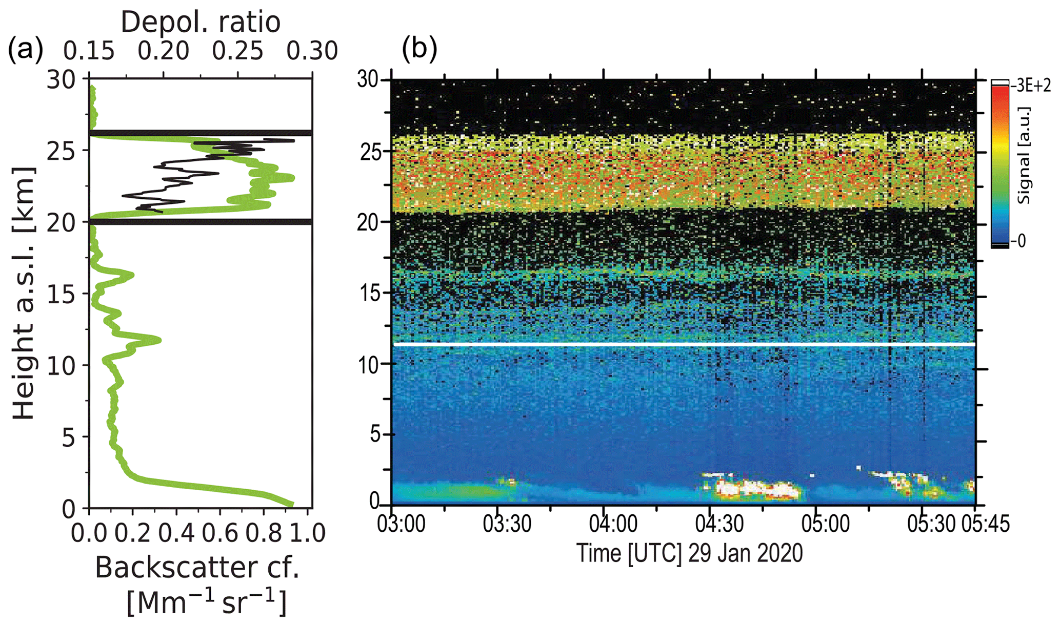
Figure 1Australian bushfire smoke (yellow layer) in the stratosphere, almost 10–15 km above the tropopause (white line in b). The mean backscatter coefficient profile (green) and the particle depolarization-ratio profile (black, for the main layer only) for the 165 min observation are shown in the left panel. Main smoke layer base and top height are indicated by black horizontal lines in panel (a). The smoke was observed with lidar at Punta Arenas, Chile, on 29 January 2020, about 10 000 km downwind of the Australian fire areas. The range-corrected 1064 nm lidar return signal is shown.
The methodological background of the conversion of optical into microphysical particle properties is given by Mamouri and Ansmann (2016, 2017). It is out of the scope of this article to present a detailed approach of how an aerosol layer can be unambiguously identified and classified as a smoke layer. In case of single-wavelength backscatter lidars, backward trajectory analysis is the main tool to identify smoke layers and link them to the most probable fire source region. In the case of modern aerosol lidars equipped with polarization-sensitive channels and aerosol and molecular backscatter channels at several wavelengths, favorable conditions are given to identify smoke layers based on the complex set of available information on particle backscatter and extinction coefficients, depolarization ratio, and lidar ratio (Wandinger et al., 2002; Müller et al., 2005; Tesche et al., 2011; Burton et al., 2012, 2015; Giannakaki et al., 2015; Giannakaki et al., 2016; Prata et al., 2017; Haarig et al., 2018; Hu et al., 2019; Adam et al., 2020; Ohneiser et al., 2020, 2021). However, an unambiguous and accurate quantification of the smoke fraction or contribution to the measured optical backscatter and extinction properties and the separation of smoke and soil dust fractions remains difficult. Soil dust may have been injected together with the smoke by the hot fires.
Regarding the separation of smoke and dust fractions by means of the polarization lidar technique (Tesche et al., 2009, 2011; Nisantzi et al., 2014), we have to distinguish two branches. As long as the smoke-containing layers occur at low altitudes (in the lower and middle troposphere up to 5–7 km height), we can apply the traditional approach to determine the smoke fraction in dust–smoke mixtures by assuming a low smoke depolarization ratio of <0.05 and a high mineral dust depolarization ratio of 0.31. In the lower and middle troposphere, aging of the smoke particles is usually fast, including the development of a spherical shape of the aged smoke particles. Furthermore, most of the smoke particles are liquid (at least the shell) at comparably high temperatures and moisture levels. All this leads to a low smoke depolarization ratio at all laser wavelengths from 355 to 1064 nm (Haarig et al., 2018).
However, if the smoke is lifted directly into the upper troposphere and lower stratosphere (UTLS), the smoke properties and aging features may be significantly different. With increasing height, and thus decreasing temperature, water vapor content, and amount of condensable gases, the aging process slows down and the smoke particles become partly glassy. These effects seem to prohibit the development of a perfect spherical shape of the shells. As a consequence, the depolarization ratio can be as high as 0.15–0.2 at 532 nm at greater heights (Burton et al., 2015; Haarig et al., 2018; Hu et al., 2019; Ohneiser et al., 2020). However, we also observed low smoke depolarization ratios in the UTLS region (Ohneiser et al., 2021). Thus, in the case of UTLS smoke observations, the dust–smoke separation technique cannot be used. We have to assume that smoke layers are dominated by smoke (smoke fraction >0.9) in the UTLS regime, and the soil dust fraction can be neglected at these heights.
To obtain height profiles of smoke in terms of volume concentration v(z), surface area concentration s(z), particle number concentrations n50(z), considering all particles with radius > 50 nm, and the large-particle number concentration n250(z), considering particles with particle radius >250 nm, we have the following four basic relationships:
with the particle backscatter coefficient β(z) at height z and the extinction-to-backscatter or lidar ratio L. The needed conversion factors cv, cs, c250, and c50 and the extinction exponent x for 532 nm are obtained from the analysis of AERONET observations during situations dominated by wildfire smoke. The results of our smoke-related AERONET data analysis are presented in Sect. 5.
An important input parameter is the smoke lidar ratio L, required to obtain the smoke extinction coefficient σ=Lβ in the first step of the conversion procedure. As discussed in the review of Adam et al. (2020), the smoke lidar ratio can vary from 25 to 150 sr at 532 nm. However, most studies show that the 532 nm lidar ratio is typically in the range of 70 sr ± 25 sr. For 355 nm, lidar ratios were mostly found around 75 ± 25 sr for fresh smoke and 55 ± 20 sr for aged smoke. Table 1 provides an overview of the large range of smoke lidar ratios. Aged smoke shows a characteristic L ratio of . This feature allows a clear unambiguous identification of smoke layers after long-range transport (Müller et al., 2005; Noh et al., 2009; Nicolae et al., 2013; Ohneiser et al., 2020). The reason for the large spectrum of lidar ratios is the complex smoke properties (size, shape, composition) as discussed in Sect. 2. Extended discussions on smoke lidar ratios can be found in Nicolae et al. (2013), Haarig et al. (2018), and Adam et al. (2020).
Haarig et al. (2018)Ohneiser et al. (2020)Wandinger et al. (2002)Murayama et al. (2004)Veselovskii et al. (2015)Alados-Arboledas et al. (2011)Nicolae et al. (2013)Mylonaki et al. (2018)Baars et al. (2012)Tesche et al. (2011)Giannakaki et al. (2015)Table 1Dual-wavelength lidar observations of lidar ratios (L) at 355 and 532 nm in tropospheric (T) and stratospheric (S) smoke layers.
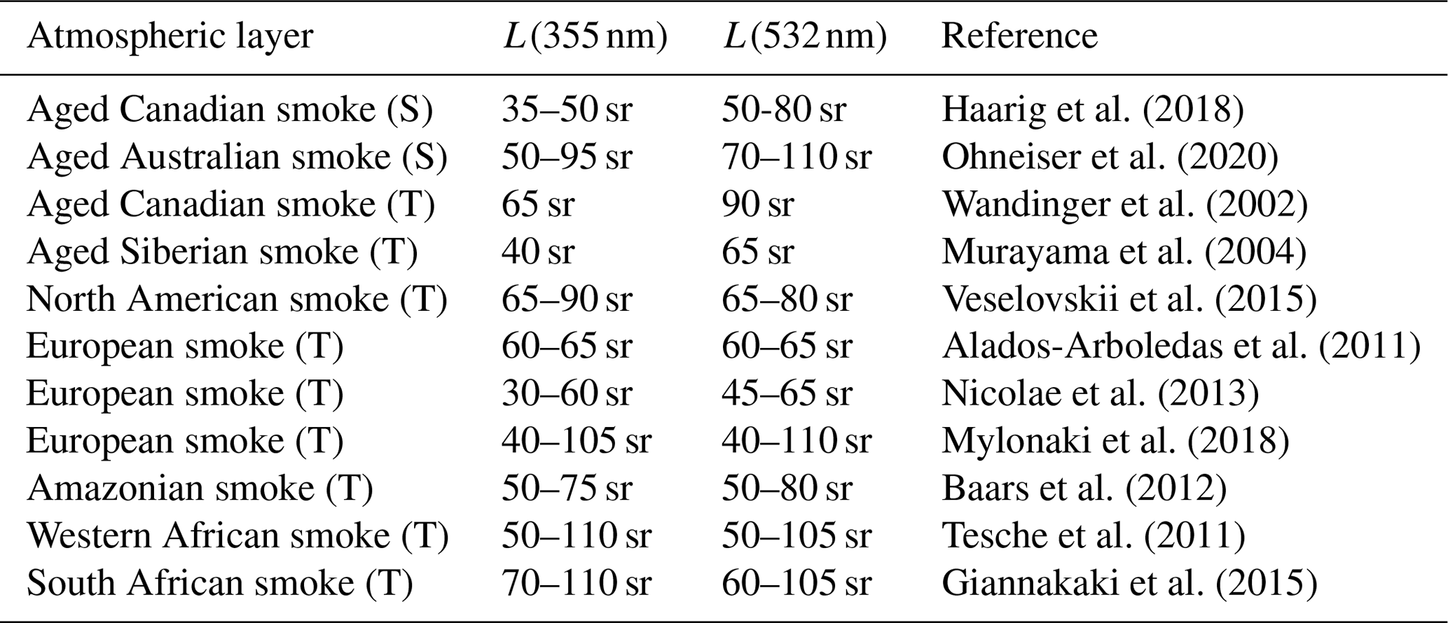
We recommend to use a lidar ratio of 55 sr for 355 nm and 70 sr for 532 nm for aged smoke if there is no possibility to obtain actual lidar ratio information from Raman lidar (Wandinger et al., 2002; Veselovskii et al., 2015; Haarig et al., 2018; Ohneiser et al., 2020, 2021) or High Spectral Resolution Lidar (HSRL) observations (Wandinger et al., 2002; Burton et al., 2015), or in the way Prata et al. (2017) proposed in the case of the CALIPSO lidar to estimate the lidar ratio of smoke layers embedded in clear air. For fresh smoke, an appropriate value for the lidar ratio seems to be 70-80 sr at both wavelengths.
From the obtained values of v, s, and n50 further relevant parameters can be calculated. The smoke mass concentration m is given by
with ρ the density of the smoke particles. Li et al. (2016) investigated different smoke aerosols in the laboratory by burning of different straw types and found densities of 1.1 to 1.4 g cm−3 for the produced smoke particles. For organic particles ρOM was about 1.05 ± 0.15 g cm−3, and for ρEC (elemental carbon) they yielded 1.8 g cm−3. Chen et al. (2017) reviewed the smoke research in China and concluded that the smoke particle density is 1.0–1.9 g cm−3. Thus in cases with 2 %–10 % of BC the overall smoke particle density should be in the range of 1.0–1.3 g cm−3.
The particle concentration n50 is a good aerosol proxy for aerosol particles serving as cloud condensation nuclei (CCN),
The CCN concentration is a strong function of updraft speed and thus water supersaturation Sw. The number concentration n50 roughly indicates the CCN concentration for weak updrafts and frequently observed low water supersaturations of Sw=0.2 %. Water supersaturation values may be in the range of 0.4 %–0.7 % in strong updrafts. Then the CCN concentration is a factor of about 2 higher than n50.
In the case of free-tropospheric and stratospheric smoke, we assume that the relative humidity in the smoke plumes is typically <60 % so that the derived n50 values represent the number concentrations for dry aerosol particles, required in the CCN estimation. The estimation of CCN concentration in cases with high relative humidity and corresponding aerosol water-uptake effects is described in Mamouri and Ansmann (2016).
The particle concentration n250 indicates the reservoir of favorable INPs and is even used as input in dust-INP parameterizations (DeMott et al., 2015). However, in the case of smoke the input parameter in the INP retrieval is the surface area concentration s,
The INP concentration is a function of s, the ice supersaturation Si (which occurs during lifting processes), and temperature T. Details of the complex INP parameterization are given in Sect. 3.1.
Finally, information on smoke particle number concentrations (n50, n250) and surface area concentration s at stratospheric heights is of interest in studies of heterogeneous formation of polar stratospheric clouds (PSCs). A significant increase in smoke aerosol particle concentration may have a sensitive impact on the evolution of PSCs and their microphysical properties (Voigt et al., 2005; Hoyle et al., 2013; Engel et al., 2013; Zhu et al., 2015).
In order to use the developed smoke retrieval formalism presented here in the case of backscatter lidars operated at single wavelengths of λ=355 or 1064 nm backscatter lidars, we need to estimate the respective backscatter coefficient at 532 nm in the first step. The 532 nm backscatter profiles within smoke layers may be estimated by using typical smoke color ratios . This aspect is further discussed in Sect. 6.
3.1 INP parameterization
As discussed in Sect. 2.2, the estimation of INP concentrations is challenging due to the chemical complexity of the smoke aerosol. The parameterizations introduced in this section cover the OM-related ice nucleation for the temperature range in the upper troposphere (C). Only for these low temperatures, organic smoke particles may be able to influence ice nucleation in the atmosphere. In the following, we present procedures to compute INP concentrations for immersion freezing, deposition ice nucleation, and homogeneous freezing.
3.1.1 Immersion freezing
Organic smoke particles that have undergone long-range transport are chemically complex, and INP parameterizations that capture the ice formation rate at upper tropospheric and lower stratospheric conditions (i.e., including subsaturated conditions) are scarce (Knopf et al., 2018). Knopf and Alpert (2013) introduced the water-activity-based immersion freezing model ABIFM, drawn from the water-activity-based homogeneous ice nucleation theory (Koop et al., 2000). Knopf and Alpert (2013) present an ABIFM parameterization for two types of humic compounds based also on experimental data by Rigg et al. (2013) that is valid for saturated and subsaturated atmospheric conditions. For demonstration of our method, we chose to apply the ABIFM for leonardite (a standard humic acid surrogate material) to represent the amorphous organic coating of smoke particles. The ABIFM allows prediction of the ice particle production rate Jhet,I as a function of ambient air temperature T (freezing temperature), ice supersaturation Si, particle surface area s, and time period Δt for which a certain level of ice supersaturation Si is given. For demonstration purposes, we simply assume a constant supersaturation period Δt of 10 min (600 s). Such supersaturation conditions may occur during the upwind phase of a gravity wave.
According to Eqs. (6)–(8) in Alpert and Knopf (2016), we calculate the so-called water activity criterion (Koop et al., 2000) in the first step:
The term aw,i in Eq. (8),
is the ratio of ice saturation pressure Pi to water saturation pressure Pw as function of temperature T and can be accurately determined by using Eq. (7) in Koop and Zobrist (2009). When the condensed phase and vapor phase are in equilibrium, the water activity aw is equal to RHw (written as 0.75 if RHw=75 %) in the air parcel in which ice nucleation takes place (e.g., in a cirrus layer at height z at temperature T). Relative humidity and temperature values may be available from radiosonde ascents or taken from databases with re-analyzed global atmospheric data. However, the actual RHw and T values during the lifting process (associated with cooling and increase in RHw and decrease in T in the air parcel) remain always unknown and need to be estimated in the studies of a potential smoke impact on cirrus formation. The organic aerosol type leonardite needs a relative humidity over ice RHi of about 130 % or Δaw=0.2 at C to become efficiently activated as INP.
In the next step, the ice crystal nucleation rate coefficient Jhet,I (in cm−2 s−1) is calculated:
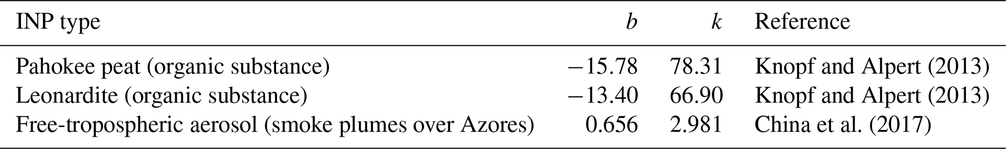
The particle parameters b and k are determined from laboratory studies for different organic aerosol material. Table 2 contains the parameters for two different natural organic substances (Pahokee peat and leonardite) (Knopf and Alpert, 2013) which serve as surrogates of the organic coating of the atmospheric smoke particles. Leonardite, an oxidation product of lignite, is a humic-acid-containing soft waxy particle (mineraloid), black or brown in color, and soluble in alkaline solutions. Both substances served as surrogates for humic-like substances (HULIS, Sect. 2.1) in extended immersion freezing laboratory studies (Knopf and Alpert, 2013; Rigg et al., 2013). Organic aerosols containing HULIS are ubiquitous in the atmosphere. We also applied the ABIFM parameterization to aerosol samples representing free-tropospheric aerosol (FTA, China et al., 2017) collected on substrates on the Azores for offline micro-spectroscopic single-particle analysis and ice nucleation experiments. According to backward trajectories, the air masses arriving at the Azores crossed western parts of North America during the main fire season (August–September). FTA showed clear smoke signatures. Note that Eq. (10) delivers strongly fluctuating solutions of Jhet,I when Δaw is small, and it delivers robust, less fluctuating Jhet,I values for Δaw>0.1.
Knopf and Alpert (2013)Knopf and Alpert (2013)China et al. (2017)Table 2Values for b and k for three organic aerosol INP types required to determine the ice nucleation rate Jhet,I with Eq. (10).
In the final step, we obtain the number concentration of smoke INP for the immersion freezing mode,
with the surface area concentration s of the smoke particles in cm2 m−3 and the time period Δt (in seconds) for which constant or almost constant ice supersaturation conditions are given. This can be the time period of a short updraft event (of a few minutes, 120–300 s) or of the lifting period of a gravity wave (>600 s). Long-lasting lifting phases of gravity waves can be up to 20 minutes (1200 s) as our Doppler lidar and radar observations conducted in several field campaigns during the last 10 years indicate.
3.1.2 Homogeneous freezing
Alternatively to smoke particles acting as heterogeneous INPs, we need to consider full deliquescence of smoke particles so that homogeneous freezing comes into play. Following Koop et al. (2000), the ice nucleation rate coefficient for homogeneous freezing is obtained from
for . The INP concentration is then obtained from
with the particle volume concentration v in cm3 m−3. Homogeneous freezing proceeds at RHi≈150 % at −50 ∘C (i.e., Δaw≈0.31), whereas 130 % (Δaw=0.2) is required at −50 ∘C to activate leonardite-containing particles. Thus at slow ascent conditions heterogeneous ice nucleation on smoke particles may dominate ice formation in cirrus layers.
3.1.3 Deposition nucleation
Wang and Knopf (2011) provide a simplified parameterization of deposition ice nucleation (DIN) based on classical nucleation theory that describes the DIN efficiency of humic and fulvic acid compounds as a function of ambient temperature T and the humidity parameters RHi and Si. An alternative DIN parameterization is provided by, e.g., Hoose et al. (2010). A detailed description of the approach presented here is given in Sect. 3.6 in Wang and Knopf (2011), and thus only a brief introduction is given in the following.
The INP efficiencies are expressed as a function of the contact angle Θ, which describes the relationship of surface free energies among the three involved interfaces including water vapor, ice embryo, and INP. Θ is parameterized as a function of RHi (Eq. 8 in Wang and Knopf, 2011).
The compatibility parameter mΘ=cos (Θ) (expressing the match between ice embryo and INP) is then used to determine the so-called geometric factor fg(mΘ) (Eq. 7 in Wang and Knopf, 2011), the free energy of ice embryo formation (Eq. 6 in Wang and Knopf, 2011), and finally the ice crystal nucleation rate Jhet,D (Eq. 5 in Wang and Knopf, 2011) in cm−2 s−1,
with the Boltzmann constant kB. The final step is then
In terms of the contact-angle-based approach, represents the case of homogeneous ice nucleation. The smaller Θ, the greater the propensity of the INP to act as deposition nucleation INP.
At the end of this section it remains to be emphasizes that we put together several INP parameterizations in Sect. 3.1 for demonstration purposes. The research on the smoke impact on atmospheric ice formation is ongoing (Knopf et al., 2018). Presently, uncertainties in the prediction of Jhet,I and Jhet,D for organic aerosols are very high (Wang and Knopf, 2011; China et al., 2017). However, the procedures introduced above allow us to estimate INP concentration profiles for organic aerosols and to study the potential impact of wildfire smoke on ice formation in tropospheric mixed-phase and ice clouds. In the upcoming years, strong field activities are required, including comparisons of airborne in situ with lidar observations of smoke INP concentrations as successfully performed in the case of Saharan dust (Schrod et al., 2017; Marinou et al., 2019) and so-called cirrus closure experiments as realized in the case of cirrus formation in pronounced Saharan dust layers (Ansmann et al., 2019b) in order to check the applicability of developed smoke INP parameterizations and to quantify the uncertainties in the INP estimates under real-world meteorological, cloud, and aerosol conditions. A first closure study with respect to smoke–cirrus interaction was recently presented by Engelmann et al. (2020).
The AERONET database (AERONET, 2021) contains unique multiyear climatological data sets of spectrally resolved aerosol optical properties and related underlying microphysical properties of aerosol particles (e.g., size distribution, volume, and surface area concentration). These AERONET products are available in the database for purely marine, dust, biomass-burning smoke, and anthropogenic haze conditions as well as for complex mixtures of these basic aerosol types. We used the advantage of the AERONET database already to derive the conversion parameters for marine and Saharan dust conditions (Mamouri and Ansmann, 2016, 2017) and extended the dust-related study later on to many desert dust regions around the world (Ansmann et al., 2019a). Now, we apply the methodology to the wildfire aerosol type.
4.1 AERONET sites
The smoke conversion parameters cv, cs, c50, c250, and x, required to solve Eqs. (1)–(4), were determined from sun photometer observations at nine AERONET stations, distributed over several continents. Figure 2 shows the considered AERONET stations. The observations at these sites cover the full range of smoke scenarios, from fresh to aged plumes, for different fire types and burning material, and smoke occurrence in the troposphere and stratosphere.
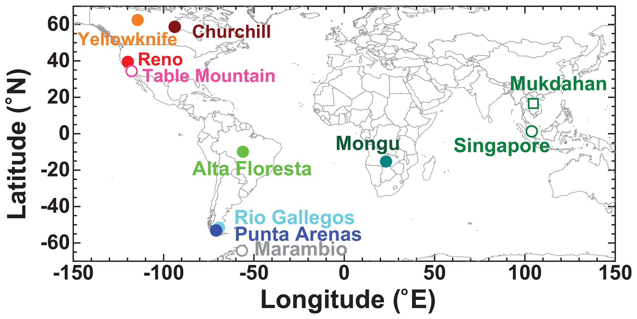
Figure 2AERONET stations used in our study. Aged stratospheric smoke from the major Australian bush fires was observed over the South American and Antarctic stations (Rio Gallegos, Punta Arenas, Marambio) in January and February 2020. Fresh and aged stratospheric smoke from record-breaking fires in British Columbia, Canada, were measured over Yellowknife and Churchill, respectively, in August 2017. Mixtures of fresh and aged tropospheric smoke originating from strong fires in the western United States and Canada were found over Reno and Table Mountain in late August to mid-October 2020. AERONET stations at Alta Floresta, Mongu, Mukdahan, and Singapore have long, multiyear data records of smoke observations in key regions of biomass burning.
Yellowknife (AERONET site: Yellowknife Aurora) and Churchill in Canada were selected because these AERONET sites were located in the outflow region of major smoke plumes which originated from the record-breaking wildfires in British Columbia (Hu et al., 2019; Baars et al., 2019; Torres et al., 2020), Canada, in August 2017. Strong pyrocumulonimbus (pyroCb) towers (Fromm et al., 2010) developed and lifted enormous amounts of wildfire smoke into the upper troposphere and lower stratosphere (UTLS) from 21:00 UTC on 12 August to 00:30 UTC on 13 August 2017 (Peterson et al., 2018). The smoke observation at Yellowknife and Churchill could be thus well assigned to the time after injection and allowed us to study the change in the smoke conversion parameters as a function of time from 12–18 h to about 5 d after injection.
The AERONET stations at Rio Gallegos (CEILAP-RG), Argentina; Punta Arenas (Punta-Arenas-UMAG), Chile, at the southernmost tip of South America; and Marambio in Antarctica were selected because well-aged smoke layers crossed these stations in January and February 2020 (Ohneiser et al., 2020). The smoke originated from strong fires in southeastern Australia and traveled the 10 000 km distance within 8–12 d. Strong pyroCb activity lifted the smoke layers up to UTLS heights, and self-lifting processes (Boers et al., 2010) caused further ascent to heights 10–20 km above the tropopause (Ohneiser et al., 2020; Kablick et al., 2020; Khaykin et al., 2020). The background AOT levels are clearly below 0.05 at 532 nm at these high northern and southern mid-latitudinal stations, far away from industrialized centers, so that the smoke layers could be clearly identified and dominated the sun photometer observations over many days (Yellowknife, Churchill) and weeks (Punta Arenas, Rio Gallegos, Marambio).
In order to consider several centers of biomass burning of global importance we selected six further AERONET stations. Smoke from exceptionally strong forest fires in the western United States and western Canada was observed over Reno (University of Nevada, Reno), Nevada, and Table Mountain (Table Mountain, CA), California, from the end of August to mid-October 2020 (in close distance to the fire sources) and allowed the determination of conversion parameters for very fresh and mixtures of fresh and aged North American tropospheric smoke layers.
We downloaded long-term observations performed at the AERONET stations Alta Floresta, Brazil (Amazonian forest fires); Mongu, Zambia, in southern Africa; Mukdahan, Thailand; and Singapore in Southeast Asia to consider observations in key fire areas of global importance. The Mongu data sets consists of sun photometer observations at the Mongu site from 1997–2009 and at the Mongu Inn site from 2013–2019. Fairly constant burning conditions are given at Mongu from July to November of each year. The long-term observations in the Amazon region, southern Africa, and Southeast Asia cover smoldering and flaming fires, fresh and aged smoke layers, and agricultural, grassland, savannah, peat, forest, and bush fires. The selection of these AERONET stations in key burning areas was guided by the smoke study of Sayer et al. (2014).
The AERONET smoke studies are supplemented by multiwavelength lidar observations of smoke conversion parameters. These vertically resolved observations were performed at Punta Arenas, Chile (Ohneiser et al., 2020); Manaus, Brazil (Baars et al., 2012); near Washington, DC (Veselovskii et al., 2015); at Cabo Verde; in the outflow regime of central western African smoke (Tesche et al., 2011), at Leipzig and Lindenberg, Germany (Wandinger et al., 2002; Haarig et al., 2018); and on the German icebreaker Polarstern drifting through the high Arctic close to the North Pole during the winter half year of 2019–2020 (Engelmann et al., 2020; Ohneiser et al., 2021). The lidar results are shown in Sect. 5.5. The retrieval of the microphysical properties was based on backscatter coefficients measured at 355, 532, and 1064 nm and extinction values at 355 and 532 nm (Müller et al., 1999a, b; Veselovskii et al., 2002), except for the smoke observations over Lindenberg in the summer of 1998. Here, particle backscatter coefficients at six wavelength (355, 400, 532, 710, 800, 1064 nm) and extinction coefficients at 355 and 532 nm were available (Wandinger et al., 2002).
4.2 AERONET data analysis
We used the version-3 level-2.0 inversion AERONET products (AERONET, 2021) in the case of the long-term observations in the Amazon region, southern Africa, and Southeast Asia and level-1.5 data in the case of the remaining stations. The reason for using level-1.5 data was to significantly increase the number of available observations in our smoke-related studies. Many observations showing high to very high smoke AOTs could not pass the strict criteria of the AERONET data quality checks and were thus removed from the level-2.0 data set. We compared the level-2.0 AERONET products with the corresponding (reduced) level-1.5 products to guarantee that the used level-1.5 data set was of high quality.
In agreement with the AERONET data analysis of Sayer et al. (2014), we used the fine-mode AOTs stored in the AERONET database. Smoke particles form a well-developed accumulation mode (with sizes up to about 1 µm in radius) and the related optical properties are assigned as fine-mode AERONET products (Sayer et al., 2014). However, as will be discussed in Sect. 5.1, a bimodal distribution (accumulation plus coarse mode) was often retrieved from the AERONET sun and sky observations. This was also pointed out by Sayer et al. (2014). The second mode is probably related to soil, road, and desert dust or marine aerosol in the planetary boundary layer. The comparison with respective lidar observations clearly indicates that smoke produces a pronounced accumulation mode only. A coarse mode is absent. Thus, we computed the smoke-related values of s, v, n50, and n250 from the downloaded size distributions by considering the size classes 1–11 only (covering the accumulation mode and thus the radius range up to 0.9–0.95 µm) and correlated these calculated microphysical values with the fine-mode AOT at 532 nm as stored in the AERONET database to finally obtain the conversion parameters. Details of the computation of s, v, n50, and n250 from the AERONET size distributions can be found in Mamouri and Ansmann (2016, 2017).
We begin the discussion of the AERONET results with an overview of the smoke measurements at Yellowknife and Churchill (stratospheric smoke), Reno and Table Mountain (tropospheric smoke), and at Punta Arenas, Rio Gallegos, and Marambio (stratospheric smoke) in Fig. 3. The downloaded AOT data sets (AERONET, 2021) contain values of fine-mode, coarse-mode, and total AOT for 440, 675, 870, and 1020 nm. The AOT τ for 532 nm is obtained from the 440 nm AOT τ440 and the Ångström exponent a by
The Ångström exponent a is defined as with wavelengths λ of 440 and 675 nm. We separately computed 532 nm AOT for fine-mode, coarse-mode, and total aerosol size distributions by using respective fine, coarse, and total aerosol Ångström exponents. In Fig. 3, the total, i.e., fine-mode plus coarse-mode, AOT is shown. In all other figures below, we exclusively used the fine-mode AOT at 532 nm. In cases with a strong smoke occurrence, the fine-mode fraction is usually >0.9.
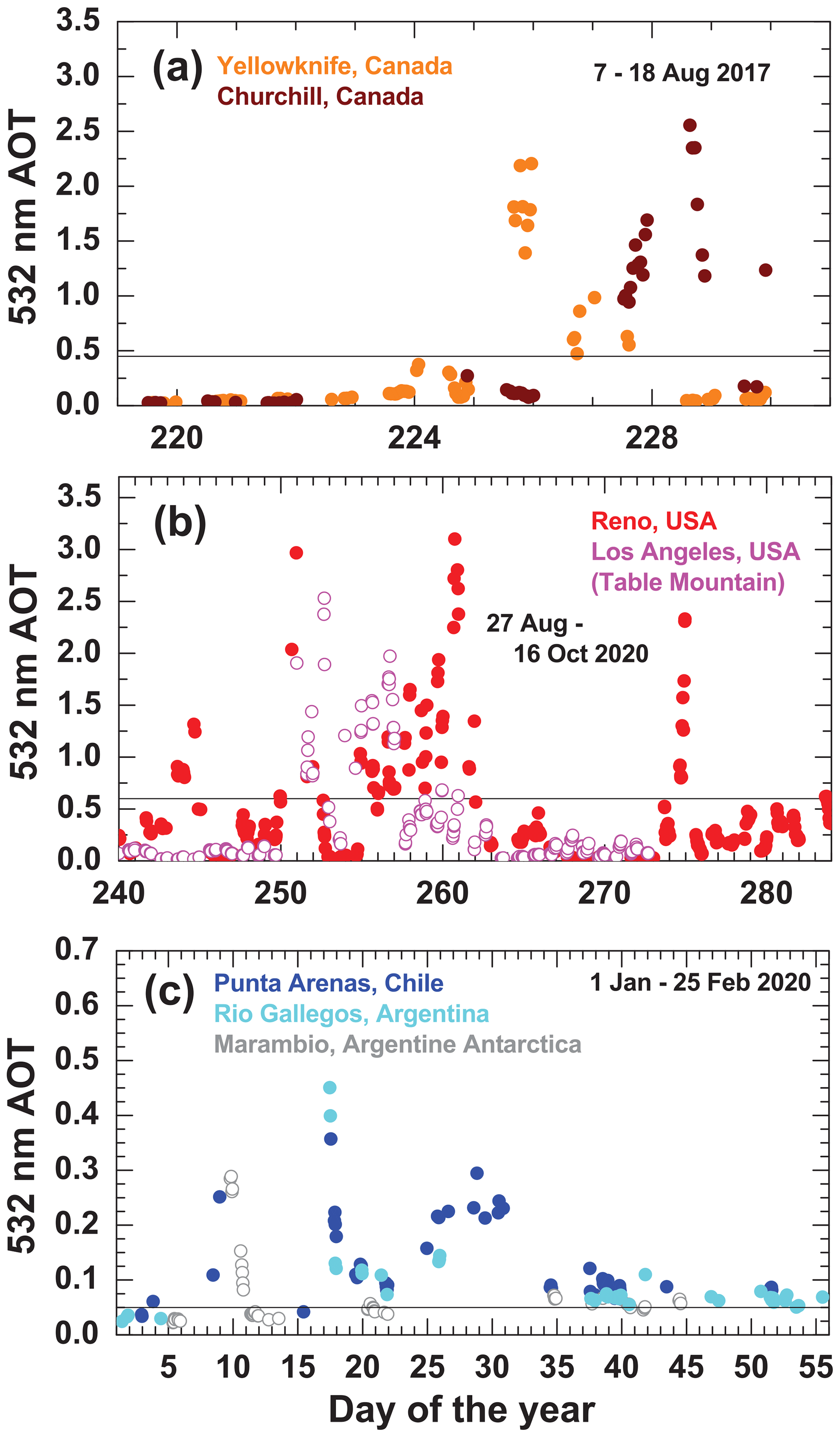
Figure 3AERONET observations of strong smoke plumes in terms of 532 nm AOT: (a) optically dense stratospheric smoke layers over northern-central Canada after the major pyroCb-related fire event in British Columbia, Canada, in the afternoon of 12 August 2017 (day 224), (b) tropospheric smoke over the western United States during major forest fires in the late summer and early autumn of 2020, and (c) aged stratospheric smoke over southern South America and Antarctica in January and February 2020 about 10 000 km east of the Australian wildfires sources. The horizontal lines indicate the minimum AOT values considered in the determination of the conversion parameters. The smoke-free background 532 nm AOT levels are (a) 0.025–0.05, (b) 0.1–0.25, and (c) 0.025–0.035.
The measurements at Yellowknife and Churchill in Fig. 3a were performed 0.5–2.5 d and 2–5 d after injection of smoke into the UTLS height range over British Columbia, Canada, respectively. The injection took place between 21:00 UTC on 12 August 2017 and 00:30 UTC on 13 August 2017 (Peterson et al., 2018). As can be seen, the first smoke plumes arrived over Yellowknife, Canada, already 12–18 h after injection. The 532 nm AOT reached values of almost 2.5. The smoke plumes traveled southeastward and crossed Churchill about 1.5–4 d later. A maximum AOT of 2.7 was measured over Churchill. At clean background conditions the AOT is about 0.025 to 0.05 at these Canadian AERONET stations. To consider all smoke observations over Yellowknife from 13–15 August 2017 (days 225–227) we set the AOT threshold level to 0.45; i.e., we considered cases with total 532 nm AOT of ≥0.45, only, in our conversion study.
Rather strong fires occurred in California during the late summer and early autumn of 2020 (Fig. 3b). Mixtures of fresh and aged smoke were observed over Reno and Table Mountain. We increased the 532 nm total AOT threshold level to 0.6 to avoid a significant impact of urban haze on the wildfire smoke observations and derivation of smoke conversion parameters. The haze-related AOT was about 0.1–0.25. The exclusive use of the AERONET fine-mode products further eliminated the potential impact of non-smoke aerosol such as coarse dust and marine particles on the correlation studies.
Figure 3c shows the observations of aged Australian wildfire smoke in southern South America and northern Antarctica. The smoke traveled more than 10 000 km within 8–12 d before reaching our combined lidar and AERONET station at Punta Arenas (Ohneiser et al., 2020). The diluted smoke caused 532 nm AOTs mostly between 0.05 and 0.3. Maximum values were close to 0.5. At clean background conditions, the AOT is in the range from 0.025–0.035. In our smoke-related AERONET data analysis, we considered all observations with AOT > 0.05 and again carefully checked that all used cases, even those with low AOT, showed clear and dominating smoke signatures (i.e., a pronounced accumulation mode). We selected the low AOT threshold of 0.05 to have sufficient cases in our conversion study for well-defined aged smoke. For each of the shown AOT observation in Fig. 3 we downloaded the required size distributions and computed the respective column-integrated values of scol, vcol, n50,col, and n250,col (by considering the size classes 1–11).
To obtain the smoke extinction-to-volume conversion factor cv,
required to derive volume and mass concentrations with Eqs. (1) and (5), the ratio of the vertically integrated (column) particle volume concentration vcol to the fine-mode 532 nm AOT τ was formed for each individual smoke observation. To facilitate the lidar-related discussion we divided the column values by an arbitrary layer depth D (length of the vertical column) and obtain
with the layer mean volume concentration v and the layer mean particle extinction coefficient σ. The introduced layer depth D has no impact on the retrieval of the conversion factors and is only introduced to move from column-integrated values and AOT to more lidar-relevant quantities like concentrations and extinction coefficients. In this study, we set D=1000 m as in the studies before (Mamouri and Ansmann, 2016, 2017).
For each smoke observation j (from number j=1 to J), available in the AERONET database, we computed cv,j and then determined the mean value, which we interpret as a representative smoke conversion factor,
In the same way, the conversion factors c250, needed to estimate the large-particle number concentration with Eq. (3), and cs, required in the surface area retrieval with Eq. (2), were computed:
It is noteworthy to emphasize again that only the accumulation-mode size range (radius classes 1–11) was considered in the computation of n250 and s.
In the retrieval of the conversion parameters required to obtain n50 (Eq. 4), we used a different approach (Mamouri and Ansmann, 2016). Following the procedure suggested by Shinozuka et al. (2015), we applied a log–log regression analysis to the log(n50,j)–log(σj) data field and determined in this way representative values for c50 and x that fulfill best the relationship,
We begin the result section with a discussion of observed smoke size distributions in Sect. 5.1. The continuous growth of smoke particles during the first days after emission is linked to a continuous change in the conversion factors. Therefore, the conversion parameters are significantly different for fresh and aged smoke. In Sect. 5.2, we then present the results of the AERONET-based correlation analysis, starting with the most simple scenarios of well-defined aged smoke observed over the AERONET stations in southern South America and northern Antarctica. Afterwards, we illuminate the link between the microphysical properties v, s, n50, and n250 and the measured light-extinction coefficient σ for mixtures of fresh and aged smoke in North America (Sect. 5.3) and over the subtropical and tropical stations in South America, southern Africa, and Southeast Asia (Sect. 5.4). In addition, in Sect. 5.5, we compare the AERONET findings with lidar observations of smoke conversion factors. The lidar-based approach is an independent method to determine microphysical properties from measured optical effects and thus provides a favorable opportunity to check the relationship between microphysical and optical properties of smoke layers as obtained from the AERONET analysis.
5.1 Smoke particle size distributions: from fresh to aged smoke
As emphasized in Sect. 2, the particle size distribution of smoke particles changes with time during the first days after injection into the atmosphere as a result of particle aging processes (chemical processing, particle collisions, and coagulation). The changing size distribution has a strong influence on the microphysical and optical properties as well as the correlation between v, s, n50, and n250 and the smoke extinction coefficient σ.
Figure 4 provides insight into the full range of size distributions of atmospheric smoke particles. The smallest particles found at Alta Floresta indicate rather fresh smoke, probably just a few hours after emission. The size distributions for Yellowknife (measured on 13 August 2017, 23:18 UTC) and Churchill were observed about 20 h and 3.5 d after injection of smoke into the UTLS height region, respectively. Aged smoke after long-range transport over more than 1 week was observed at Punta Arenas (8 d after emission) and Lindenberg (10.5 d after emission). It is obvious that the size distribution is shifted towards larger particles with increasing residence time in the atmosphere. All size distributions are normalized so that the integral over each shown size distribution is one. Lidar observation conducted at Leipzig, 180 km to the southwest of Lindenberg (Haarig et al., 2018), and over Punta Arenas (Ohneiser et al., 2020) agree well with the respective AERONET size distributions. The lidar observations corroborate that the smoke size distribution is unimodal.
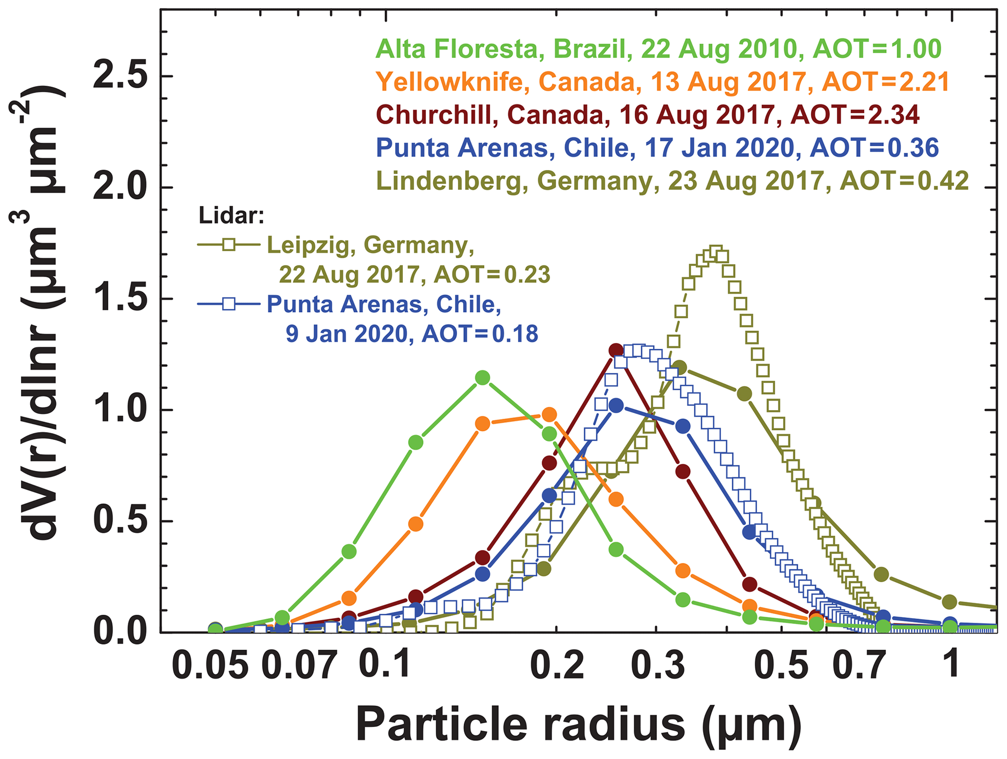
Figure 4Comparison of normalized volume size distributions of smoke particles highlighting the shift of the size distribution towards larger particles with age of the observed smoke. The Amazonian smoke size distribution (Alta Floresta, green) is indicative for rather fresh smoke. Canadian smoke over Yellowknife (orange), Churchill (red), and Lindenberg (brown) was observed 1, 3–4, and 10–11 d after injection of smoke into the UTLS. The Punta Arenas observation (blue) was taken after about 8 d of long-range transport. The stratospheric size distributions obtained from lidar observations (open symbols, Punta Arenas, Leipzig) match well with the respective AERONET observations at Punta Arenas and Lindenberg (about 180 km northeast of Leipzig). The accumulation-mode radius shifted from 150–200 nm (Yellowknife) to 300–400 nm (Lindenberg) within the 9 d travel of the 2017 smoke plumes from Yellowknife in Canada to Germany.
Figure 5 shows unimodal as well as bimodal size distribution in cases clearly dominated by smoke. Similar bimodal size distributions were presented in the smoke study of Sayer et al. (2014). The weak coarse mode may result from aerosols in the boundary layer (marine particles, soil, and road dust). The lidar observations do not show this coarse mode.
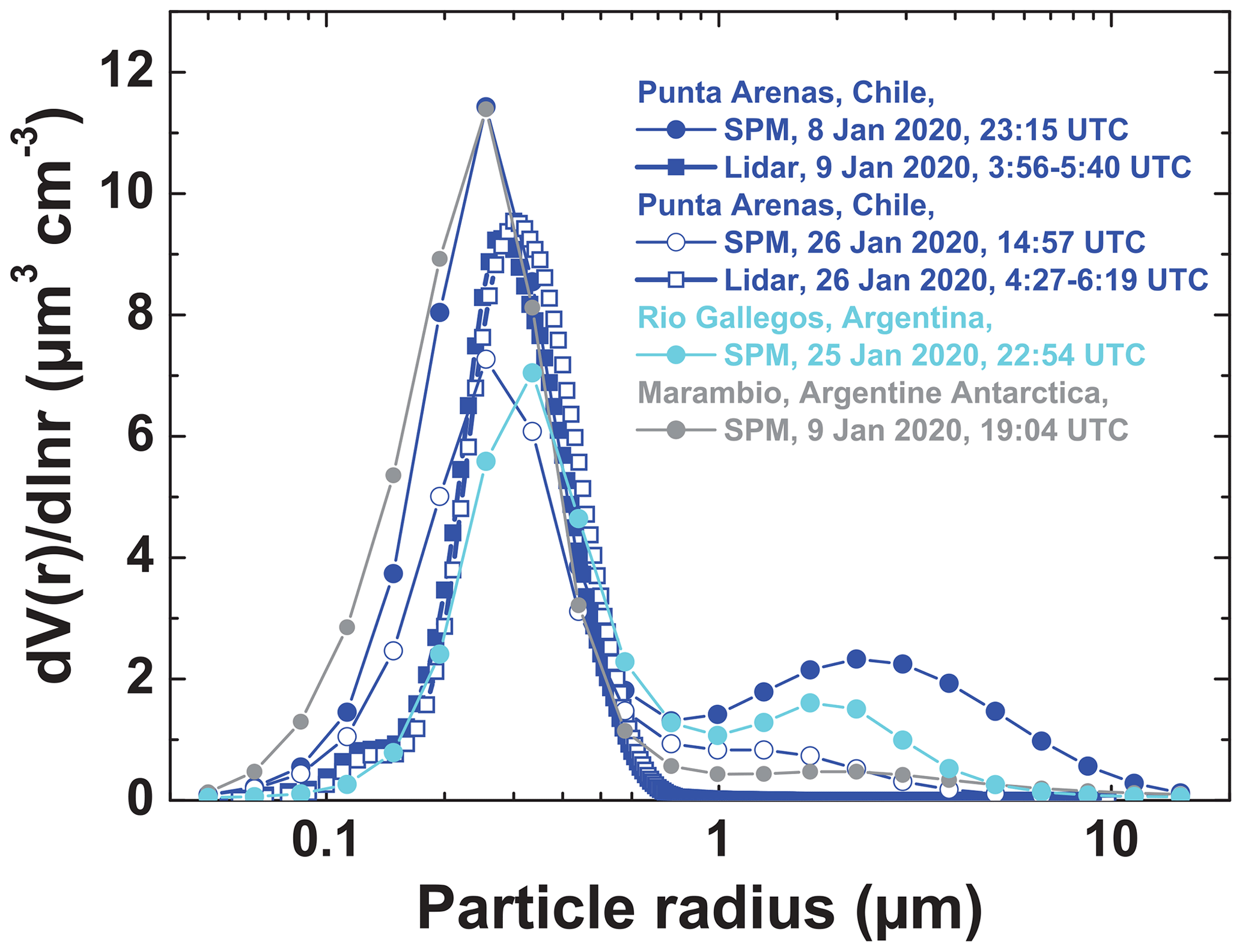
Figure 5Normalized volume size distributions of smoke particles derived from column (tropospheric + stratospheric) AERONET sun photometer (SPM) observations at Punta Arenas, Rio Gallegos, and Marambio in January 2020. In addition, size distributions obtained from the inversion of lidar-derived optical properties (squares) in the well-defined smoke layers are shown. Base and top heights of the smoke layers were 12.8 and 15.7 km on 9 January 2020 and 19.3 and 22.9 km on 26 January 2020, respectively. The lidar-derived size distributions show an accumulation mode only; a distinct coarse mode is absent.
To consider the changing smoke size distributions shown in Fig. 4 in the smoke data analysis, it would be desirable to have conversion parameter sets for fresh, weakly aged, and aged smoke particles. However, in all likelihood such an approach would be impractical and/or unreasonably difficult. As will be discussed below in detail, the majority of AERONET smoke observations close to the fire regions indicate that fresh smoke was usually mixed with enhanced levels of background aerosol which, to a large extent, consists of aged smoke. This regional background aerosol obviously builds up over the fire regions during the long-lasting fire seasons. Therefore, we decided to distinguish just between two different measurement scenarios: (a) aged smoke observations (smoke observed after long-range transport over 5 d and more) and (b) measurements of mixtures of fresh and aged smoke (in the near-range to large fire areas). For these two scenarios we developed conversion parameterizations.
5.2 AERONET results for aged smoke
Figure 6 shows the relationship between (a) the smoke volume concentration v and the smoke-related extinction coefficient σ, (b) particle surface area concentration s and σ, and (c) the particle number concentration of larger smoke particles n250 and σ for aged Australian smoke. The correlation between the number concentration n50 and σ is discussed in Sect. 5.6. As a general impression, a clear relationship between v, s, and n250 and σ is found, at least up to extinction coefficients of 300 Mm−1 (or 0.3 in terms of the fine-mode AOT at 532 nm). The spread in the data reflects variations in the smoke properties (size distribution, refractive index). However, the relatively low scatter in the data is a sign for large similarities in the smoke properties (observed over several weeks). This may be related to the fact that the flaming-fire type prevailed, eucalyptus trees were the main burning material, smoke lifting was always linked to strong pyroCb activity and thus similar lifting features, and the size distributions of aged smoke particles after 8–12 d long-range transport are at all very similar.
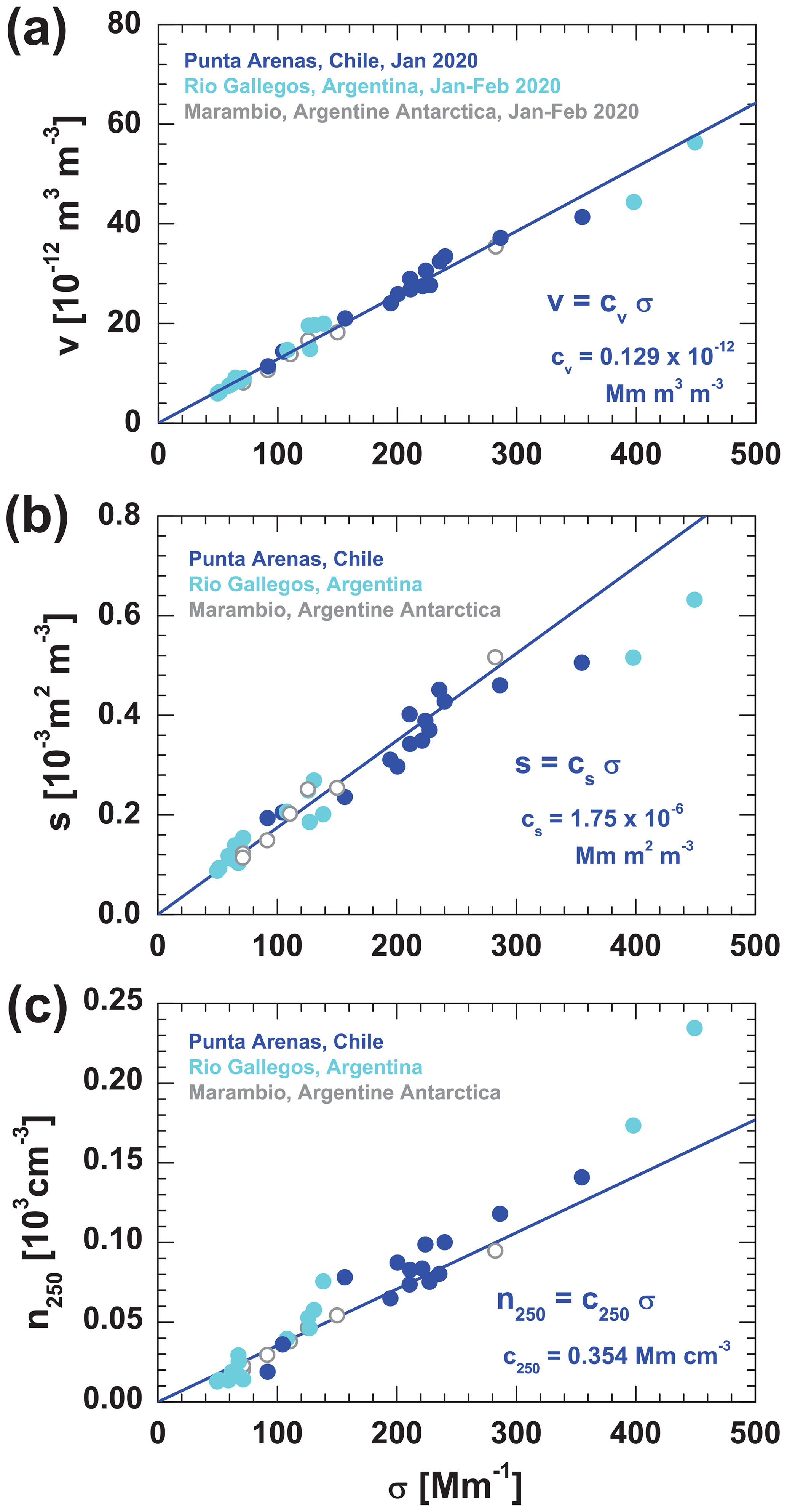
Figure 6Relationship between smoke extinction coefficient σ (532 nm) and (a) volume concentration v, (b) surface area concentration s, and (c) number concentration n250 of aged stratospheric Australian smoke observed over the three AERONET stations in South America and Antarctica. The slopes are defined by the equations in the different panels (a), (b), and (c). The conversion factors cv, cs, and c250 in these equations are the mean values of the observed individual ratios of (Eq. 19), (Eq. 21), and (Eq. 20). These mean values are given as numbers in the panels and together with the corresponding standard deviations also in Table 3.
The mean relationships between v, s, and n250 and σ are visualized by straight blue lines. The respective mean conversion factors cv, cs, and c250 are given as numbers in the different panels and also summarized in Table 3. These mean conversion factors were computed from the data in Fig. 6a, b, and c by using the Eqs. (19), (21), and (20), respectively.
5.3 AERONET results for mixtures of fresh and aged North American smoke
Figure 7 presents the correlations between the smoke volume concentration v and the smoke extinction coefficient σ (Fig. 7a) and between the smoke surface area concentration s and the smoke extinction coefficient (Fig. 7b) for North American forest fires. The forests in the western United States and Canada mainly consist of pine, fir, aspen, and cedar trees. The flaming-fire type probably prevailed in August 2017 and August–October 2020. The observations in Fig. 7 cover fresh and aged smoke plumes as well as mixtures of both. Strong variations in the size distribution are reflected in the comparably large scatter in the data. The upper part of the data fields shows cases dominated by fresh smoke (smaller particles) and the lower part, around the blue regression line for aged smoke (from Fig. 6), is dominated by aged smoke (larger particles). Nevertheless, a clear relationship between the computed volume and surface area concentrations and the measured smoke extinction coefficient is given.

Figure 7Same as Fig. 6a and b, except for fresh (Yellowknife) and aged stratospheric smoke (Churchill) in August 2017 and for mixtures of fresh and aged tropospheric smoke over Reno and Table Mountain, mostly observed in September and October 2020. The red lines are calculated with the equations given in panels (a) and (b). They consider Yellowknife and Reno data, only. The conversion factors cv (Eq. 19) and cs (Eq. 21), again the mean values of all individual observations of the ratios and , are given as numbers. The blue lines (taken from Fig. 6) are shown for comparison.
We used the observations at Yellowknife (1–2 d old stratospheric smoke) and Reno (tropospheric smoke, observed a few hours to several days after injection) to compute the conversion parameters and mean relationships visualized by red solid lines in Fig. 7. The mean values of cv and cs, as given in the figures, were calculated with Eqs. (19) and (21). Only the Yellowknife and Reno data in Fig. 7 were considered in this computation. All mean conversion factors are summarized in Table 3.
The Yellowknife data points (fresh smoke) are close the red lines. This may indicate that the respective conversion factors (given as numbers in Fig. 7) describe predominately fresh and weakly aged North American smoke properties. The blue straight lines (for aged Australian smoke) seem to define the lower limit of the range of values in Fig. 7. Many observations taken at Table Mountain, east of Los Angeles (tropospheric smoke), and at Churchill (2–5 d old stratospheric smoke) are close to the blue lines for aged smoke.
5.4 AERONET results for mixtures of fresh and aged Amazonian, African, and Southeast Asian smoke
In this section, we switch from short-term observations of record-breaking and major fire episodes to long-term observations (partly over decades) in key burning areas of global importance. We assume that these long-term observations cover the full range of smoke-property-influencing aspects (smoldering and flaming fires, very different fuel types, short- to long-range smoke transport, and related smoke aging effects). Figure 8 presents the correlations between the computed smoke values of the volume concentration v and surface area concentration s and the smoke-related fine-mode extinction coefficient σ at 532 nm for all four selected subtropical and tropical stations. A relatively strong variability is found for the relationship between the surface area concentration and extinction coefficient in Fig. 8b, and even significant differences between the different data sets (Southeast Asian vs. African and Amazonian observations) are visible. In contrast, a quite narrow distribution of all observations is given for the volume-to-extinction relationship in Fig. 8a.
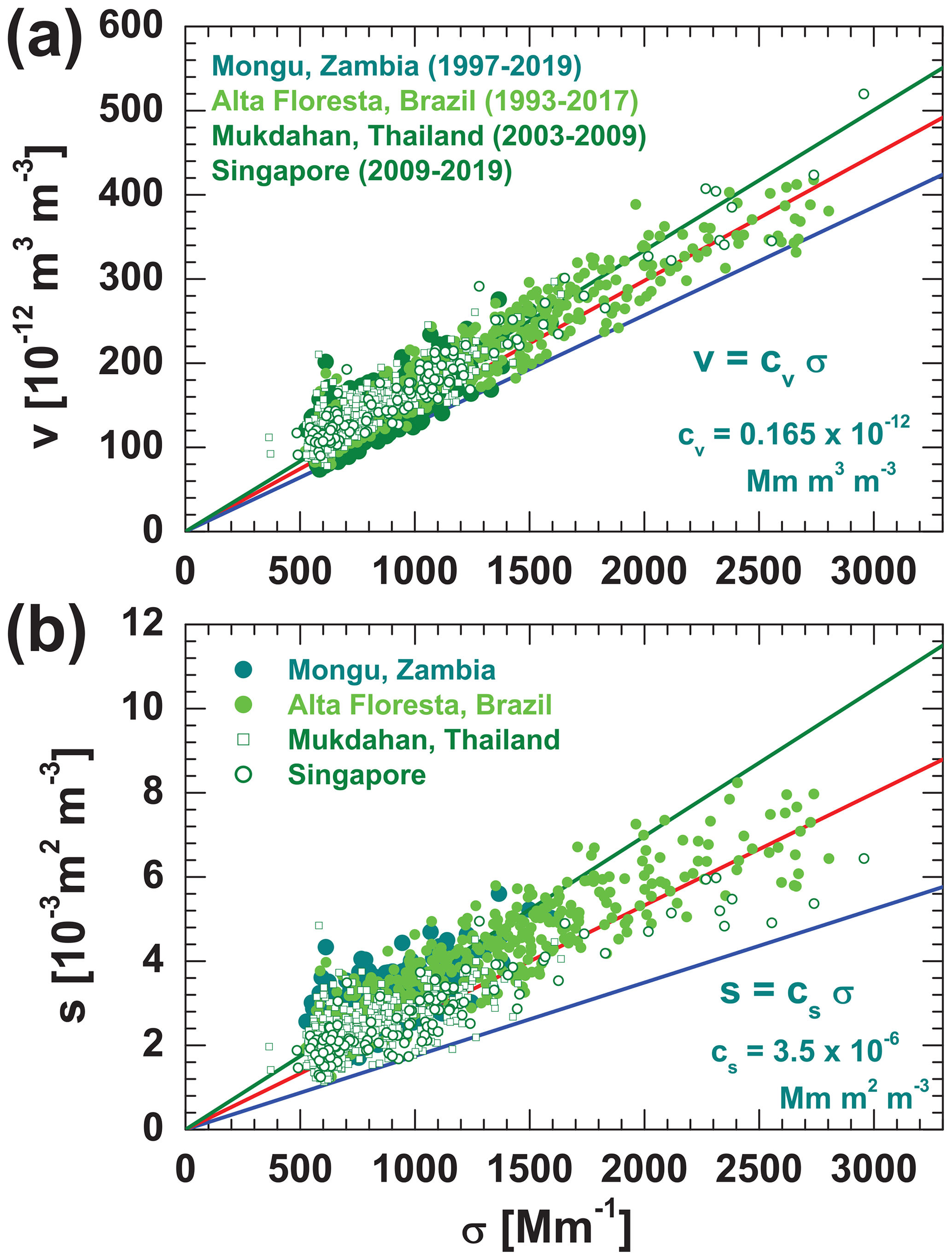
Figure 8Same as Fig. 6a and b, except for African (Mongu), Amazonian (Alta Floresta), and Southeast Asian smoke (Mukdahan and Singapore: open olive circles for Mukdahan data and open olive squares for Singapore data). The long-term, multiyear observations cover a wide range of burning material, fire conditions, and observations of fresh and aged smoke properties. The slopes (green lines, for the Mongu data set) are defined by the equations in the two panels (a) and (b). The conversion factors cv and cs in these equations are the mean values of the observed individual ratios of (Eq. 19) and (Eq. 21). These mean values for the Mongu site are given as numbers. The blue and red lines (taken from Figs. 6 and 7) for aged Australian smoke (blue) and mixtures of fresh and aged North American forest fire smoke (red) are shown for comparison.
The spread in the data is again widely a function of the size distribution and thus of the age of the smoke layers. As in Fig. 7, the upper part of the data fields is strongly influenced by smaller particles and thus fresh smoke, whereas the lower part is controlled by larger particles and thus aged smoke.
The green straight lines show the mean regression lines for the Mongu, Zambia, data set. The computation of the mean conversion factors is performed in the same way as described in the forgoing sections. We included again the mean regression lines for aged Australian smoke (blue lines) and also for comparably fresh North American smoke (red lines) in Fig. 8. It is obvious that the blue lines for aged smoke indicate the lower boundary of the data range in Fig. 8a and b well. On the other hand, the upper boundary of the data field seems to be less well defined. Obviously many of the observed plumes of tropical and subtropical fires, especially over Zambia and the Amazon region, are just a few hours old, and thus the smoke particles were very small. The smoke particles of the Amazon region, southern Africa, and Southeast Asia are frequently considerably smaller than North American smoke particles (represented by the red lines in Fig. 8).
It is noteworthy to mention that Sayer et al. (2014) analyzed the relationship between the column smoke volume concentrations vcol and the 550 nm fine-mode AOT τ550 for a large number of AERONET stations around the world with strong impact of wildfire smoke and found similar mean values for the ratio as given for the extinction-to-volume conversion factor cv in our figures and in the summarizing Table 3. The study of Sayer et al. (2014) includes also Russian stations (Moscow, Tomsk, Yakutsk). We may thus conclude that our conversion parameter set well covers main aspects and characteristics of wildfire smoke layers around the world.

Figure 9Same as Fig. 6a and b, except for a correlation between (a) lidar-derived v and σ and (b) lidar-derived s and σ. The closed dark green stars indicate lidar observation of fresh and aged western African smoke taken in January and February 2008. The open green and red stars show lidar observations in Brazil and the USA of mixtures of fresh and aged smoke during the summer seasons of 2008 and 2013, respectively. The two open blue triangles (Punta Arenas), three open squares (Lindenberg, Leipzig, Germany), and the black circles in the lower-left corner (North Pole region) are representative for aged smoke. The thick blue, red, and green lines show the mean increase in v and s with σ for aged Australian smoke (blue), mixtures of fresh and aged North American forest fire smoke (red), and mixtures of fresh and aged southern African smoke (green).
5.5 AERONET vs. lidar smoke observations
Lidar provides an independent approach to derive microphysical parameters of smoke and thus to determine the link between the retrieved microphysical and measured optical properties of smoke particles (Müller et al., 1999a, 2014; Veselovskii et al., 2002, 2012). This option provides the favorable opportunity to check the quality and robustness of our results obtained by analyzing the AERONET data. One of the main problems of sun photometer observations is that the entire vertical column is observed so that, e.g., boundary-layer aerosols can be a disturbing factor in the study of lofted tropospheric and stratospheric smoke plumes. These problems are absent in the case of profiling techniques such as lidar. In the case of active remote sensing methods, the optical and microphysical properties are exclusively determined for the smoke layers. However, the uncertainties in the lidar retrievals can be large, and thus the obtained data products can scatter over a wide range just as a function of these uncertainties.
In Fig. 9, lidar data sets of smoke observations from 53∘ S (Punta Arenas) to 86∘ N (North Pole range) are considered. Correlation between v and s values and σ for fresh and aged smoke plumes originating from fires in western Canada, eastern Siberia, southeastern Australia, eastern United States, the Amazon Basin, and central western Africa are shown. The AERONET-derived mean relationship between v, s, and n250 and σ for aged, fresh, and the long-term African observations as discussed in the foregoing sections are shown again as blue, red, and green lines.
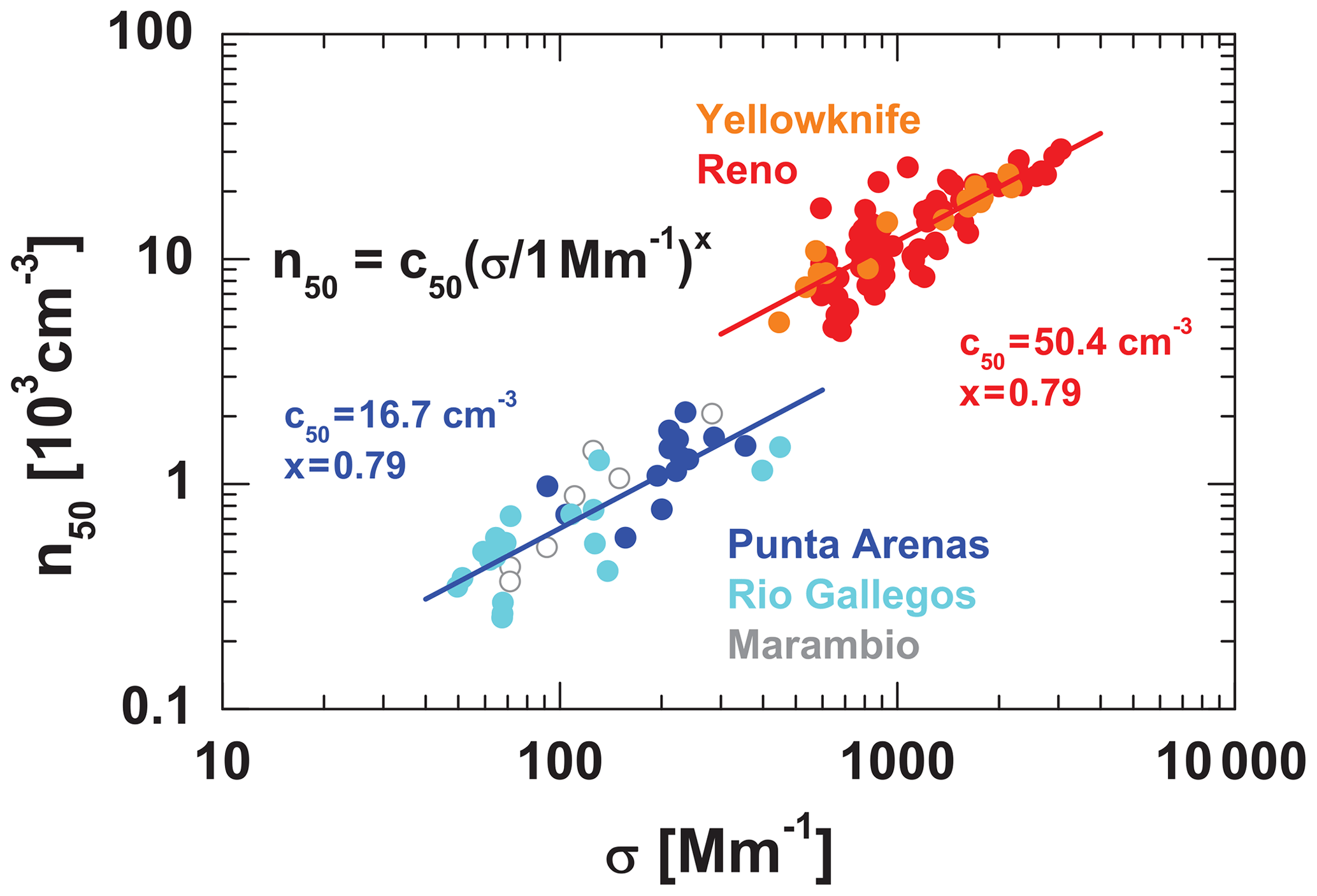
Figure 10Relationship between smoke extinction coefficient σ (532 nm) and particle number concentration n50 for the combined Reno and Yellowknife data set (fresh and aged smoke) and the combined South American and Antarctic data set (aged smoke).
A large scatter in the lidar-based smoke correlation values is visible in Fig. 9 with data points even below the blue lines and above the green lines. This large scatter is partly related to the specific retrieval methodology and data analysis strategy as well as to varying assumptions in the analysis of the different lidar data packages. The most robust results (less sensitive to input errors) are obtained in terms of surface area concentrations when using the inversion algorithm of Müller et al. (1999a, b). This method was applied to the lidar observations at Praia, Cabo Verde; Manaus, Brazil; and Lindenberg, Germany. The other observations taken at Leipzig, Punta Arenas, and the North Pole region were analyzed by applying the analysis scheme of Veselovskii et al. (2002).
In Fig. 9b, it can be seen that most of the smoke layers observed over Praia (smoke from central western Africa) contain aged smoke particles (the data points are close to the blue line), and only a minor part of the observations indicate fresh smoke plumes (these data points are close to the green line). Many smoke layers contained a mixture of fresh and aged smoke. All the lidar data, representing smoke after long-range transport (Lindenberg, Leipzig, North Pole, Punta Arenas), are close to the blue line for aged smoke or even below this line and thus in good agreement with the AERONET-based correlation studies. From the consistency found in the correlations shown, based on AERONET and lidar observations, we can conclude that the AERONET smoke conversion parameters presented here allow trustworthy retrieval of smoke microphysical properties from backscatter lidar observations.
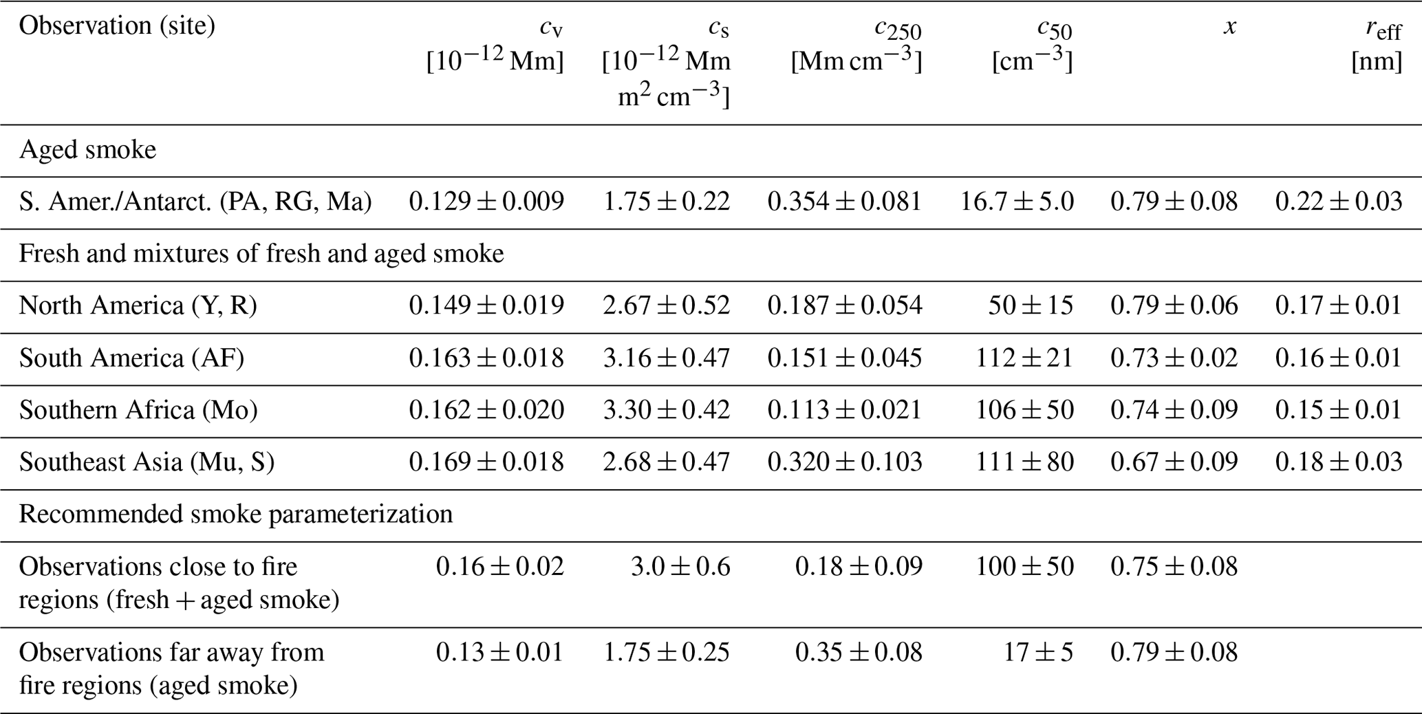
Table 3Smoke conversion parameters required in the conversion of the particle extinction coefficient σ at 532 nm into particle number concentrations n50 and n250, surface area concentration s, and volume concentration v. The mean values and SD for cv, cs, c250, c50, and x are obtained from the extended AERONET data analysis. Effective radius reff information is given as well. The conversion factors are derived from the AERONET observations at Yellowknife (Y), Reno (R), Alta Floresta (AF), Punta Arenas (PA), Rio Gallegos (RG), Marambio (Ma), Mongu (Mo), Mukdahan (Mu), and Singapore (S). The conversion parameters for South America (AF), southern Africa (Mo), and Southeast Asia (Mu, S) consider observations with AOT > 0.9 at 532 nm only.
5.6 AERONET results: n50 retrieval
Figure 10 shows the correlation between the CCN-relevant particle number concentration n50 and the extinction coefficient σ for two contrasting smoke data sets, i.e., for the observations of aged Australian smoke and, on the other hand, for the observations of fresh smoke (Yellowstone) and mixtures of fresh and aged smoke (Reno). According to the applied regression analysis, fresh smoke plumes contain much more CCN-relevant small particles (roughly a factor of 3 more) than aged plumes. For a given extinction coefficient of σ=100 Mm−1, n50 is 635 cm−3 (for aged Australian smoke over Punta Arenas), 1900 cm−3 (for North American smoke), and 3200 cm−3 (for Mongu, Zambia). The numbers for n50 and the extinction exponent x (see Eq. 4) in Fig. 10 and Table 3 are obtained by considering the respective data sets shown in the figure or mentioned in the table in the linear regression analysis described in Sect. 4.2.
Table 3 provides an overview of the derived mean conversion parameters for the different AERONET observational data sets, discussed in the foregoing section. Since the smoke size distribution widely controls the derived conversion parameters, we added the information on the effective radius, which is the particle-surface-area-weighted mean radius of the smoke accumulation mode and can be regarded as a typical radius of the observed smoke particles. For aged smoke, the effective radius is largest. It is much lower for the mixtures of fresh and aged smoke. We recommended the use of the two conversion parameter sets in the lower part of Table 3 in the analysis of smoke layers observed with backscatter lidars.
In Table 4, the uncertainties in the input parameters and the smoke retrieval products are listed. The uncertainties in the conversion parameters are estimated from the SD values in Table 3. The relative uncertainties in the required smoke lidar ratio L and smoke particle density ρ follow from the discussions in Sect. 3. Three scenarios of lidar backscatter profiling are compared in Table 4. In the case of a Raman lidar or a HSRL, the determination of the particle backscatter coefficient in clearly identified smoke layers is possible with high accuracy (10 % relative uncertainty) as our experience shows (Wandinger et al., 2002; Veselovskii et al., 2015; Haarig et al., 2018; Ohneiser et al., 2020, 2021). In addition, the lidar ratio L is measured with a typical relative uncertainty of around 20 %. In the case of a powerful ground-based elastic-backscatter lidar, the smoke lidar ratio must be estimated in the determination of the extinction coefficient. The lidar ratio is even required as input in the basic determination of the backscatter coefficient profiles. The backscatter profile retrieval may be possible with a relative uncertainty of 15 %. In the case of comparably weak backscatter signals measured from space (e.g., with the CALIPSO lidar), we assume an uncertainty of 25 % in Table 4 in the profiling of the backscatter coefficient. Details of the uncertainties in the CALIPSO aerosol backscatter coefficients are given in Young et al. (2013, 2018). Finally, the relative uncertainties in the smoke microphysical retrieval products are obtained by error propagation applied to Eqs. (1)–(5) in Sect. 3.
Table 4Relative uncertainties in the conversion input parameters (upper part of the table) and in the retrieved smoke products (lower part of the table). Fresh stands for mixtures of fresh and aged smoke (or for near-source smoke). Aged denotes well-aged smoke (or smoke after long-range transport). Different lidar systems (Raman lidar/HSRL, ground-based elastic backscatter lidar, and spaceborne elastic backscatter lidar) and thus different uncertainties in the backscatter and lidar ratio profiles are considered. The uncertainties in the conversion factors and extinction exponents are estimated from Table 3. The smoke extinction coefficient is defined as σ=Lβ.
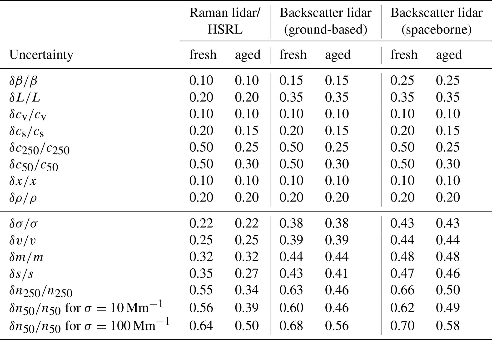
As can be seen in Table 4, the retrieval of volume, mass, and surface area concentrations of detected smoke layers is possible with an overall uncertainty of about 25 %–35 % (for both fresh or near-source smoke and for aged smoke after long-range transport) in the case of Raman lidars or HSRLs, when the smoke lidar ratios are measured. The respective uncertainties are 40 %–50 % when smoke profiling is performed with an elastic backscatter lidar so that the lidar ratio L needs to be estimated. The number concentrations n50 and n250 can be only roughly estimated with a typical uncertainty of about 50 %–70 %. Again, the retrieval uncertainties are lowest when measurements are performed with a ground-based Raman lidar or a HSRL. The uncertainties are then of the order of 35 %–50 % in the case of aged smoke.
Uncertainties in the estimates of CCN and INP concentrations are not listed in Table 4. Comparisons with airborne in situ observations of CCN profiles suggest that the uncertainty in the lidar-based CCN estimation is around 50 %, and in extreme cases up to a factor of 2 (−50 % to 100 %) (Düsing et al., 2018; Haarig et al., 2019; Genz et al., 2020). In the case of INP estimations, it is too early for an in-depth uncertainty analysis. A considerable number of dedicated field campaigns and further laboratory studies are needed before a trustworthy quantification of uncertainties in the INP estimation is possible (see also the discussion at the end of Sect. 3.1).
At the end of the section it should be mentioned that the developed method (here for 532 nm) can be applied to single-wavelength 355 and 1064 nm backscatter lidar observations as well. We recommend in these cases to estimate the 532 nm backscatter profiles from the measured 355 or 1064 nm backscatter profiles by using properly estimated smoke color ratios and (the index denotes wavelength in nm). Extended overviews of observed wavelength dependencies of smoke backscatter coefficients can be found in Burton et al. (2012) and Adam et al. (2020). In a follow-on project, we may repeat the procedure presented here for 532 nm for the wavelength of 355 nm to cover spaceborne 355 nm HSRL lidar observations of the European Space Agency. Such an approach was already presented by Mamouri and Ansmann (2016, 2017) in the case of the marine and Saharan dust types.
We applied the new smoke conversion scheme to two contrasting smoke observations. In Fig. 1, an aged stratospheric Australian smoke layer was shown, observed with an advanced multiwavelength Raman lidar (Polly: portable lidar system) (Engelmann et al., 2016) at Punta Arenas, Chile, in January 2020. This case will be further analyzed in Sect. 7.1. As a second contrasting example, we selected a measurement of the spaceborne CALIPSO lidar over North and South Dakota, USA. A comparably fresh tropospheric smoke layer was detected in September 2020. The smoke originated from strong wildfires in the western part of the United States and Canada. This case study is presented in Sect. 7.2.
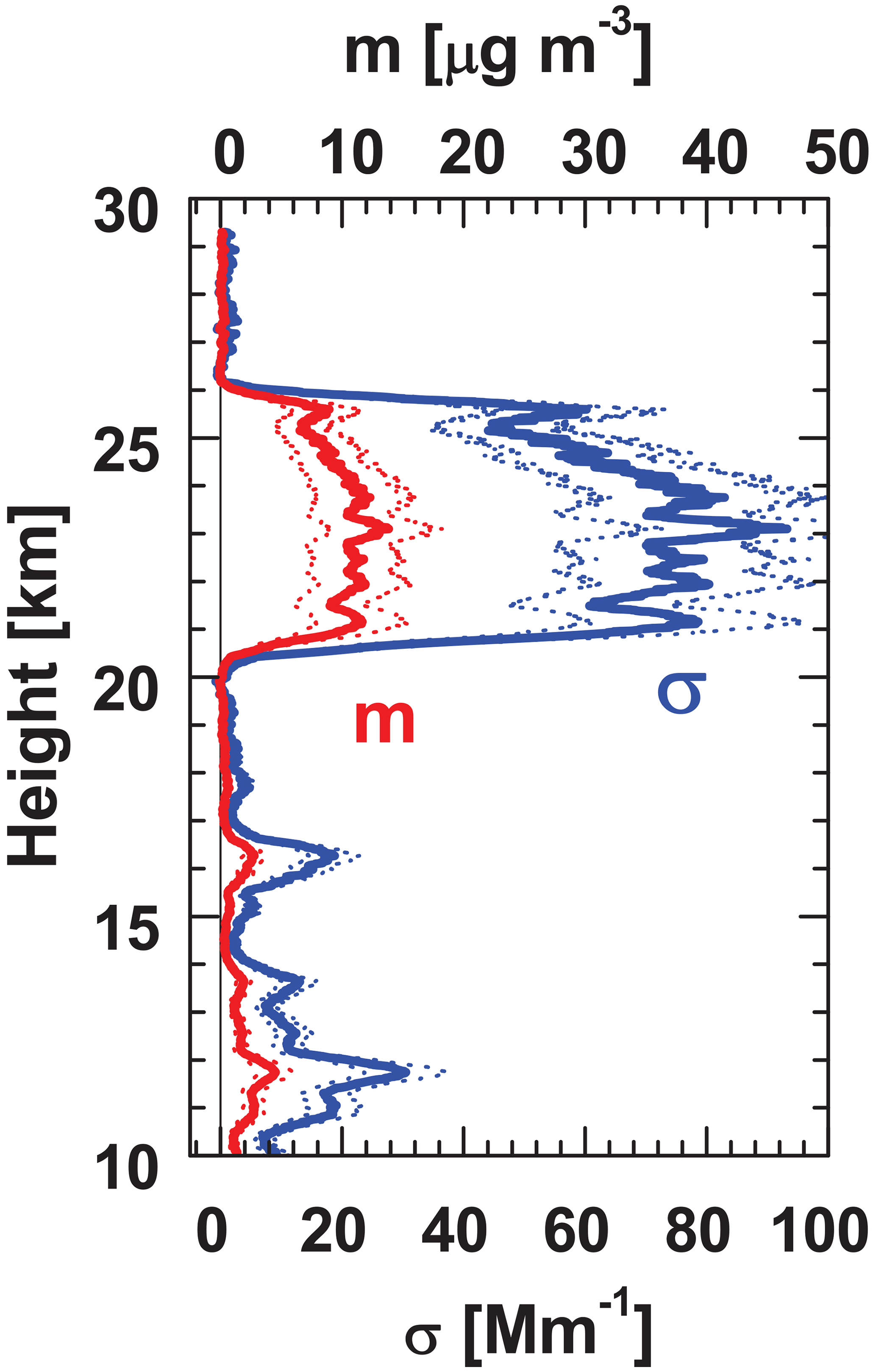
Figure 11Smoke observation with lidar in the stratosphere over Punta Arenas on 29 January 2020 (see Fig. 1) in terms of the smoke extinction coefficient σ and particle mass concentration m. Extinction coefficients were obtained by multiplying the respective backscatter coefficients with a lidar ratio of 95 sr. The errors margins (thin dotted) indicate relative uncertainties as given in Table 4 for the Raman lidar option in the case of aged smoke.
7.1 Aged Australian smoke in the stratosphere observed with ground-based Raman lidar
In the framework of a multiyear measurement campaign, we monitored the stratospheric perturbation caused by the record-breaking Australian bushfires with a polarization Raman lidar Polly over a full year, starting in January 2020 (Ohneiser et al., 2020). A measurement example is shown in Fig. 1. The results obtained by applying the conversions scheme in Sect. 3 are presented in Figs. 11–13. In the first step, we calculated the extinction coefficients from the 532 nm backscatter coefficients by using a smoke lidar ratio of L=95 sr as measured with the Raman lidar Polly (Ohneiser et al., 2020). Then we applied the conversion factor cv in Table 3 for aged smoke to obtain the volume concentration v. By assuming a particle density of ρ=1.15 g cm−3 for the smoke particles, we obtain the mass concentration m shown in Fig. 11.

Figure 12Retrieval results for 29 January 2020 in terms of surface area s and particle number concentration n50 (proxy for CCN) with error margins representing the uncertainties as given in Table 4 for the Raman lidar option in the case of aged smoke.
Such a high aerosol pollution level of 15 µg m−3 at heights from 20–26 km height has never been observed in the stratosphere before, not even after major volcanic eruptions (Trickl et al., 2013; Sakai et al., 2016). Stratospheric background levels are of the order of 0.01 µg m−3 (Baars et al., 2019; Taha et al., 2021). As shown in Fig. 1, the particle depolarization ratio was significantly enhanced as a result of fast lifting by pyroCb clouds over the Australian fire regions (Ohneiser et al., 2020). The aging process was obviously not fully completed and the particles were probably glassy. This may explain the deviation from the perfect spherical shape of the particles and the enhanced depolarization ratios (Gialitaki et al., 2020).
Figure 12 shows the derived surface area concentration s and the particle number concentration n50. Information on number concentrations and surface area at stratospheric heights is of interest, e.g., in PSC and ozone research. A record-breaking ozone depletion was observed in the stratosphere over Antarctica starting in September 2020 (CAMS, 2021). PSC particles play a strong role in this context because they permit the activation of chlorine components (on the surfaces of the PSC particles) which subsequently destroy ozone molecules. Even if we assume a strong decay of the stratospheric smoke perturbation by a factor of 10 or 100 in the Southern Hemisphere (at mid- to high latitudes) from January 2020 to September 2020, and thus a reduction in the smoke number concentration from about 500 cm−3 in Fig. 12 (in the height range from 21 to 25.5 km height) to 50 or even 5 cm−3, such number concentrations are still high and are in the range of particle concentrations typically observed in PSCs (0.01–10 cm−3) (Jumelet et al., 2008, 2009). Smoke particles may be able to serve as nuclei in processes of heterogeneous nucleation of PSC particles (Hoyle et al., 2013; Zhu et al., 2018) and thus may influence PSC microphysical properties. On the other hand, smoke surface area concentrations of around 120-130 µm2 cm−3 in the stratospheric layer in Fig. 12 are extremely high, and even if the smoke concentration was reduced by a factor of 10 to 100 until September 2020, surface area concentrations of around 10 or around 1 µm2 cm−3 are still high and partly in the same range of typical surface area concentrations in PSC clouds (Jumelet et al., 2008, 2009) so that at least a weak influence on ozone depletion by providing surface areas for chlorine activation cannot be excluded.
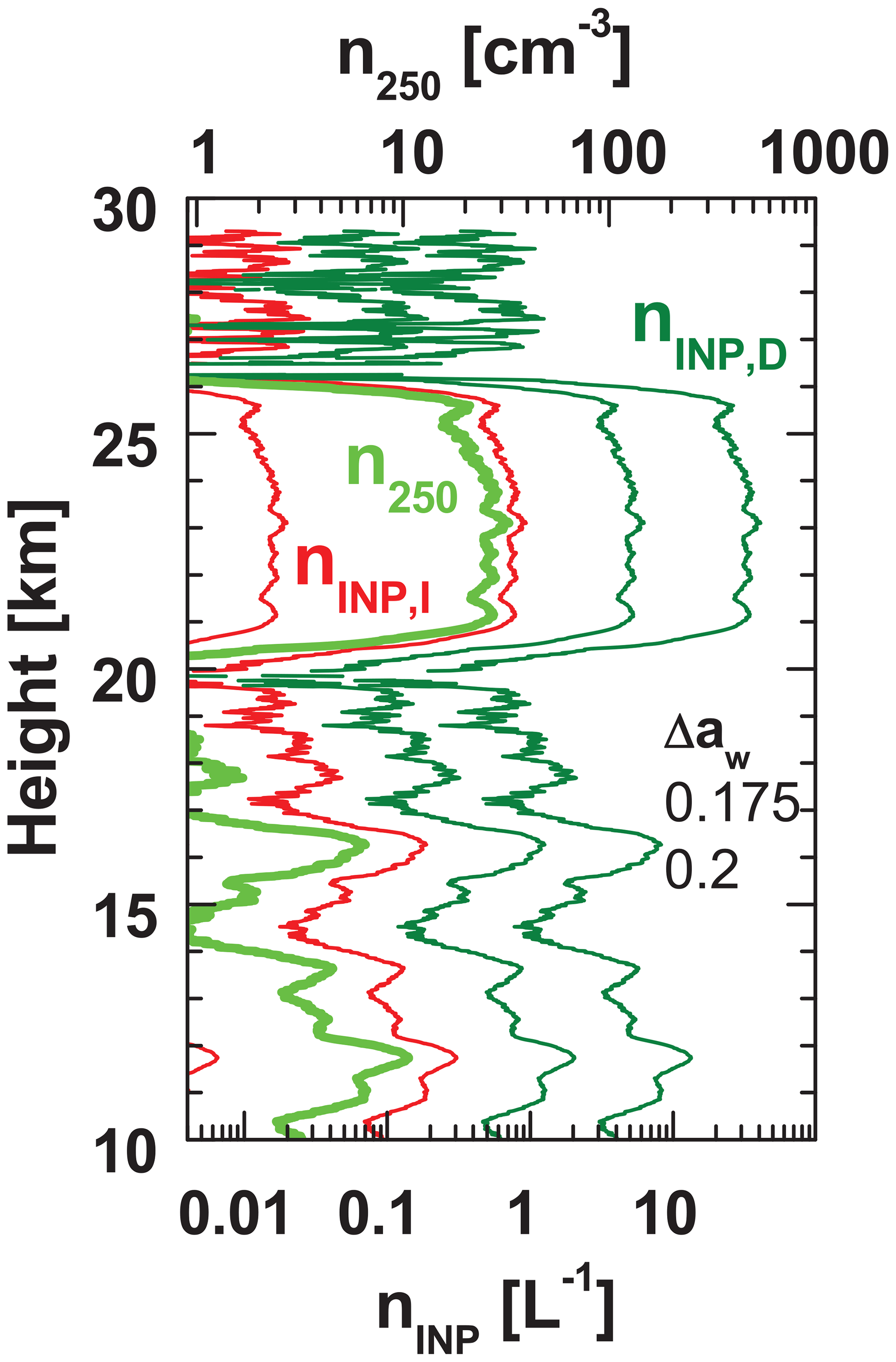
Figure 13Retrieval results for 29 January 2020 in terms of INP concentrations nINP,I and nINP,D and large particle number concentration n250 (considering particles with radius >250 nm). See text for more details of the INP computations in the case of immersion freezing (red profiles) and deposition nucleation (olive profiles). We consider leonardite as the organic aerosol substance (see Table 2). The INP concentrations are estimated by assuming an air parcel lifting period of 600 s (period of supersaturation with Δaw of 0.175 (low INP numbers) and 0.2 (high INP values)) and ice nucleation temperature of −50 ∘C.
The surface area concentration is also an essential aerosol input parameter in the INP parameterization and thus an important quantity in the research field of aerosol–cloud interaction with focus on mixed-phase-cloud and cirrus formation in the troposphere. INP estimates are shown in Fig. 13. We use the aerosol type parameters for leonardite as given in Table 2 in the calculation of immersion freezing INP (nINP,I, Sect. 3.1.1). The calculations start with the computation of the water activation criterion Δaw (Eq. 8). Ice nucleation is a strong function of the vertical velocity (lifting of moist air parcels), which leads to ice supersaturation and thus determines Δaw. In the case study here, we assume realistic upper-tropospheric cirrus formation conditions and ignore in this demonstration of INP number estimation that we observed the smoke layer in the dry stratosphere 10–15 km above the local tropopause. We assumed RHw= 79.85 % and 82.35 % and a temperature T of C. The corresponding RHi values are around 125 % and 130 %. Homogeneous freezing proceeds in significant numbers at about RHi=150 % at C. Thus, for slow air lifting, smoke particles potentially acting as INPs have a good chance to sensitively influence cirrus formation. With these input values for RHw and T, we obtain Δaw=0.175 and 0.2. The value for the ice melting point aw,i (Eq. 9) is 0.6235 at C. Afterwards, we calculated the ice nucleation rate Jhet,I (Eq. 10) and the INP concentration nINP,I (Eq. 11) by assuming a lifting period of 600 s during which ice supersaturation conditions according to Δaw of 0.175 and 0.2 are given. We also computed deposition nucleation INP solutions (nINP,D, Sect. 3.1.3) by assuming the same T, RHi, RHw, and Si input parameters together with an overall lifting period of 600 s.
Figure 13 shows the results of the nINP,I and nINP,D estimations. A strong dependence on relative humidity and ice supersaturation is visible. Obviously a threshold value of ice supersaturation Si has to be reached and exceeded before efficient immersion freezing in the case of leonardite starts. The estimated deposition nucleation INP concentration is much higher than the immersion-freezing INP values for the assumed atmospheric conditions. The obtained high INP numbers are directly correlated to the large amount of smoke particles. The obtained INP number concentrations are not too uncommon. For example, INP number concentrations reached about 10–100 L−1 in a Saharan dust plume (DeMott et al., 2003). Neglecting any radiative heating effects of the smoke layer and microphysical processes such as sedimentation and competition for water vapor, these results clearly indicate that organic smoke particles can impact ice formation processes in the upper troposphere during favorable moisture conditions and gravity wave activity with updraft phases lasting longer than several minutes.
In Fig. 13, also values for n250 (large particle fraction) are shown. It is usually assumed that particles with diameters >500 nm can be regarded as the overall reservoir for INPs (DeMott et al., 2015). Number concentrations of 10–100 cm−3 or 10 000–100 000 L−1 indicate that this reservoir of large smoke particles cannot be depleted when nINP is in the range of 0.1 to 100 L−1, not even during extended cirrus formation processes lasting several hours.
The competitive process to heterogeneous ice nucleation is homogeneous freezing. If ice supersaturation Si reaches sufficient levels, corresponding to Δaw of 0.29–0.31, nINP,hom (Eq. 13) would be of the order of 600–700 L−1 for cm3 L−1 (mean value of the 20–26 km layer).
As mentioned, the uncertainty in the INP retrieval is large and is widely related to the current status of our knowledge about smoke INP type characteristics. The lidar input parameters s and v could be obtained with low relative errors of 25 %–35 %. The research on the role of wildfire smoke particles in cirrus and PSC formation is one of the key topics in atmospheric research with focus on aerosol–cloud interaction (Knopf et al., 2018).
7.2 North American smoke in the troposphere observed with the CALIPSO lidar
Strong fires occurred in the western United States and western Canada during the late summer of 2020. The smoke even reached Europe (Baars et al., 2021). Figure 14 shows an overflight of CALIPSO from North Dakota down to Texas. Two smoke layer complexes were detected between 5 and 10 km height: one over North and South Dakota and another one over Texas. According to the backward trajectory analysis, the plumes over North and South Dakota originated from fires in western Canada and were observed after 1 d of travel from the main fire area to North and South Dakota. The plumes over Texas originated from heavy Californian fires and were observed after 3–5 d of travel time from the Californian smoke sources. Cirrus formed in the neighborhood of the smoke layers.
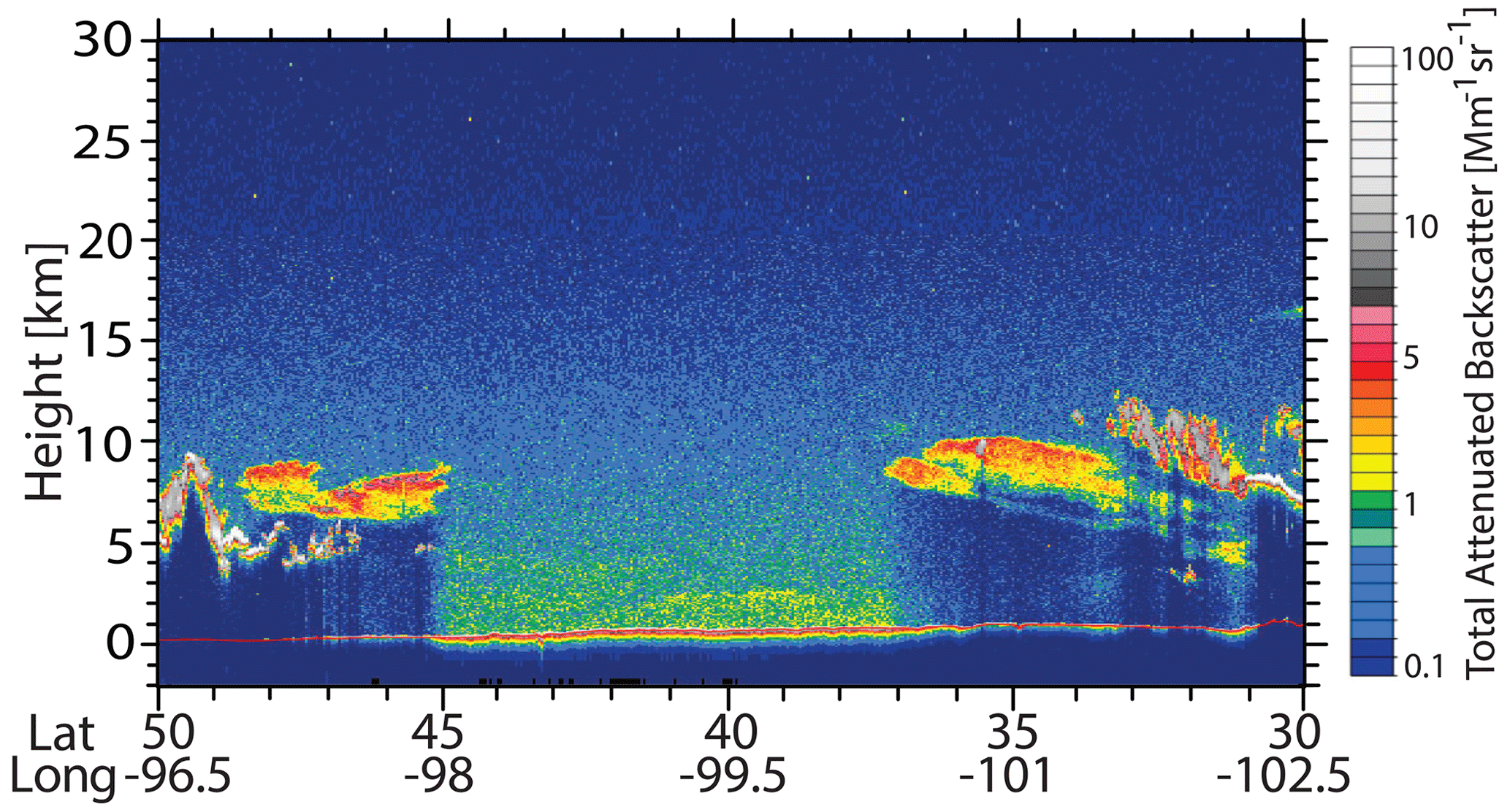
Figure 14CALIPSO lidar observations of tropospheric smoke over North and South Dakota (45–48.5∘ N, 7–9 km height) and over Texas (33–37∘ N, 8–10 km height) on 13 September 2020, around 9:15 UTC (CALIPSO, 2020a). The smoke layers (in yellow to red) originated from British Columbia (North and South Dakota plume, travel time of 24 h) and from California (Texas plume, 2–5 d of travel time) as HYSPLIT backward trajectories indicate (HYSPLIT, 2020).

Figure 15CALIPSO smoke observation in the stratosphere over North and South Dakota on 13 September 2020 in terms of (a) particle extinction coefficient σ and mass concentration m and (b) INP concentration estimates nINP,I for C, Δaw=0.2, and two different organic substances (leonardite, LEO, and free-tropospheric smoke aerosol, FTA; see Table 2). The lidar-derived input parameter is the shown surface area concentration s. The CALIPSO aerosol backscatter coefficients were downloaded and averaged over the range from 45–48.5∘ N (CALIPSO, 2020b) and then multiplied with 70 sr to obtain the extinction coefficients. Error margins (thin dotted lines) show the uncertainties in σ, m, and s as given in Table 4 (fifth column).
Figure 15 presents the height profiles of smoke extinction coefficient, mass concentration, surface area concentration, and estimated INP concentration for the smoke layers detected over eastern North and South Dakota. We used a lidar ratio of 70 sr to convert the measured smoke backscatter coefficients into extinction values and applied the conversion parameter set for fresh smoke as recommended in Table 3. A potential influence of multiple scattering was ignored. For dense aerosol layers, multiple scattering can introduce substantial unquantified errors into the CALIPSO lidar retrievals of particle backscatter and extinction coefficients (Wandinger et al., 2010; Liu et al., 2011). However, multiple scattering effects may be of the order of about 5 %–10 % (underestimation of the true extinction coefficient by 5 %–10 %) in cases with smoke layer optical thickness ≤0.5 at 532 nm (Prata et al., 2017). The particle depolarization ratio was >0.1 and thus indicated the presence of nonspherical smoke particles.
According to Table 4 (fifth column), the uncertainties in the lidar products are higher now compared to measurements with ground-based Raman lidar at Punta Arenas. Relative uncertainties of 40 %–45 % in the extinction coefficient are mainly caused by the lidar ratio assumption. The uncertainties in the mass and surface area concentrations are around 50 %.
In the computation of the immersion-freezing INP concentrations in Fig. 15b, we highlight the impact of the selected organic aerosol type (leonardite, LEO, vs. free-tropospheric aerosol, FTA, Table 2). We assumed a water activity criterion of Δaw=0.2 or RHi=130 % at C and again set the period during which ice nucleation was possible at these thermodynamic conditions to Δt=600 s. As can be seen, the assumed organic substance can have a very sensitive impact on the estimated INP values. The third organic substance in Table 2 (Pahokee peat) leads to similar INP values as obtained for leonardite. In cirrus research, it is thus essential to know the origin of the smoke and a good knowledge of the burning material to be able to properly characterize the aerosol type involved in the cloud formation studies.
We presented a new method that permits the retrieval of tropospheric and stratospheric height profiles of smoke particle mass, volume, surface area, and number concentrations as well as first-order estimates of CCN and INP concentrations from single-wavelength backscatter lidar observations. The developed smoke retrieval method is of special importance for spaceborne backscatter lidars such as CALIPSO and the numerous ground-based lidars permitting high-quality observations of height profiles of the particle backscatter coefficient at 532 nm up to stratospheric heights. The method allows us to characterize smoke microphysical and optical properties even at very low smoke pollution levels and thus during the entire decay phase of long-lasting stratospheric perturbations, from thick smoke plumes to aerosol background conditions. Even if advanced multiwavelength Raman or HSRL observations are available for the characterization of pronounced smoke layers so that the lidar inversion procedure can be applied to obtain the microphysical properties, our method based on conversion factors is useful for comparisons to corroborate the quality of the solutions obtained with advanced multiwavelength lidar systems.
The required conversion factors were determined from AERONET observations. In this approach, we distinguished observations of aged smoke and mixtures of fresh and aged smoke. A crucial task is the estimation of smoke INP concentrations because of the complex characteristics of smoke particles. Now, a consistent methodology is available to characterize wildfire smoke plumes in terms of microphysical and cloud-relevant parameters. This will allow us to study smoke–cirrus interaction as well as the potential impact of smoke particles on PSC formation and ozone depletion in large detail. We applied the new smoke analysis scheme to ground-based as well as spaceborne CALIPSO observations to highlight the potential of single-wavelength lidars (on the ground and in space) to significantly contribute to an extended monitoring and microphysical characterization of tropospheric and stratospheric smoke layers and thus to provide valuable information for climate, cloud, and air chemistry modeling efforts.
Polly lidar observations (level 0 data, measured signals) are in the PollyNET database (Pollynet, 2021) with quicklooks at http://polly.tropos.de. All the analysis products are available from TROPOS upon request (info@tropos.de). CALIPSO observations of smoke profiles and smoke AOT were used and downloaded from the CALIPSO database at https://www-calipso.larc.nasa.gov/products/lidar/browse_images/std_v4_index.php (CALIPSO, 2020a), https://search.earthdata.nasa.gov/search?fp=CALIPSO&fi=CALIOP (CALIPSO, 2020b), and https://asdc.larc.nasa.gov/project/CALIPSO/CAL_LID_L2_05kmAPro-Standard-V4-20_V4-20 (CALIPSO, 2020c). AERONET observations were downloaded from the AERONET database at http://aeronet.gsfc.nasa.gov/ (AERONET, 2021).
The paper was written by AA with contributions (data analysis, methodological concepts) from KO, REM, DAK, IV, HB, and AF. The co-authors RE, CJ, PS, and BB were involved in the field observations and took care of all the smoke measurements with the Polly lidars at Punta Arenas and aboard RV Polarstern.
The authors declare that they have no conflict of interest.
We thank AERONET for their continuous efforts in providing high-quality measurements and products. We are grateful to the present AERONET site managers Jacobo Salvador, Raul D'Elia, Ramiro Gonzales, and Jonathan Ferrarae (CEILAP-RG, Marambio); Norman O'Neill, Ihab Abboud, and Vitali Fioletov (Yellowknife, Churchill); Pam Glatfelter, Heath Rhoades, and William Buehlman (Table Mountain, California); W. Patrick Arnott and S. Marcela Loria-Salazar (Reno); Ralf Becker (Lindenberg); Edilson Bernadino de Andrade and Fernando Morais (Alta Floresta); Mukufute Mukulabai (Mongu); Anthony Daka (Mongu Inn); Surasak Meesiri, Anuson Niyompam, and Anucha Yangthaisong (Mukdahan); Tan Li (Singapore); and all previous site managers. We also thank the CALIPSO team for their well-organized easy-to-use internet platforms.
This article is part of the special issue “EARLINET aerosol profiling: contributions to atmospheric and climate research”. It is not associated with a conference.
The authors acknowledge support through the European Research Infrastructure for the observation of Aerosol, Clouds and Trace Gases (ACTRIS) under grant agreement no. 654109 and 739530 from the European Union's Horizon 2020 research and innovation program. We thank AERONET-Europe for providing an excellent calibration service. AERONET-Europe is part of the ACTRIS project. R.-E. M. has been financially supported by the SIROCCO project (grant no. EXCELLENCE/1216/0217) co-funded by the Republic of Cyprus and the structural funds of the European Union for Cyprus through the Research and Innovation Foundation. Thanks are also provided to the ERATOSTHENES Centre of Excellence, which was established after receiving funding by the Republic of Cyprus and the EU H2020 Widespread Teaming program with grant agreement no. 857510 (https://excelsior2020.eu/, last access: 20 January 2021). The field observations at Punta Arenas are partly funded by the German Science Foundation (DFG) project PICNICC with project no. 408008112. The development of the lidar inversion algorithm used to analyze Polly data was supported by the Russian Science Foundation (project 16-17-10241). D.K. acknowledges support by the DOE grant DE-SC0021034. The Polarstern Polly data were produced as part of the international Multidisciplinary drifting Observatory for the Study of the Arctic Climate (MOSAiC) with the tag MOSAiC20192020 and project ID AWI_PS122_00.
This paper was edited by Lucia Mona and reviewed by two anonymous referees.
Adam, M., Nicolae, D., Stachlewska, I. S., Papayannis, A., and Balis, D.: Biomass burning events measured by lidars in EARLINET – Part 1: Data analysis methodology, Atmos. Chem. Phys., 20, 13905–13927, https://doi.org/10.5194/acp-20-13905-2020, 2020. a, b, c, d
AERONET: Aerosol Robotic Network aerosol data base, available at: http://aeronet.gsfc.nasa.gov/, last access: 28 February, 2021. a, b, c, d
Alados-Arboledas, L., Müller, D, Guerrero-Rascado, J. L., Navas-Guzmán, F., Pérez-Ramírez, D., and Olmo, F. J.: Optical and microphysical properties of fresh biomass burning aerosol retrieved by Raman lidar, and star- and sun-photometry, Geophys. Res. Lett., 38, L01807, https://doi.org/10.1029/2010GL045999, 2011. a, b
Alpert, P. A. and Knopf, D. A.: Analysis of isothermal and cooling-rate-dependent immersion freezing by a unifying stochastic ice nucleation model, Atmos. Chem. Phys., 16, 2083–2107, https://doi.org/10.5194/acp-16-2083-2016, 2016. a, b
Ansmann, A., Mamouri, R.-E., Hofer, J., Baars, H., Althausen, D., and Abdullaev, S. F.: Dust mass, cloud condensation nuclei, and ice-nucleating particle profiling with polarization lidar: updated POLIPHON conversion factors from global AERONET analysis, Atmos. Meas. Tech., 12, 4849–4865, https://doi.org/10.5194/amt-12-4849-2019, 2019a. a
Ansmann, A., Mamouri, R.-E., Bühl, J., Seifert, P., Engelmann, R., Hofer, J., Nisantzi, A., Atkinson, J., Kanji, Z., Amiridis, V., Vrekoussis, M., and Sciare, J.: Ice-nucleating particle versus ice crystal number concentration in altocumulus and cirrus layers embedded in Saharan dust: a closure study, Atmos. Chem. Phys., 19, 15087–15115, https://doi.org/10.5194/acp-19-15087-2019, 2019b. a
Baars, H., Ansmann, A., Althausen, D., Engelmann, R., Heese, B., Müller, D., Artaxo, P., Paixao, M., Pauliquevis, T., and Souza, R.: Aerosol profiling with lidar in the Amazon Basin during the wet and dry season, J. Geophys. Res., 117, D21201, https://doi.org/10.1029/2012JD018338, 2012. a, b
Baars, H., Ansmann, A., Ohneiser, K., Haarig, M., Engelmann, R., Althausen, D., Hanssen, I., Gausa, M., Pietruczuk, A., Szkop, A., Stachlewska, I. S., Wang, D., Reichardt, J., Skupin, A., Mattis, I., Trickl, T., Vogelmann, H., Navas-Guzmán, F., Haefele, A., Acheson, K., Ruth, A. A., Tatarov, B., Müller, D., Hu, Q., Podvin, T., Goloub, P., Veselovskii, I., Pietras, C., Haeffelin, M., Fréville, P., Sicard, M., Comerón, A., Fernández García, A. J., Molero Menéndez, F., Córdoba-Jabonero, C., Guerrero-Rascado, J. L., Alados-Arboledas, L., Bortoli, D., Costa, M. J., Dionisi, D., Liberti, G. L., Wang, X., Sannino, A., Papagiannopoulos, N., Boselli, A., Mona, L., D'Amico, G., Romano, S., Perrone, M. R., Belegante, L., Nicolae, D., Grigorov, I., Gialitaki, A., Amiridis, V., Soupiona, O., Papayannis, A., Mamouri, R.-E., Nisantzi, A., Heese, B., Hofer, J., Schechner, Y. Y., Wandinger, U., and Pappalardo, G.: The unprecedented 2017–2018 stratospheric smoke event: decay phase and aerosol properties observed with the EARLINET, Atmos. Chem. Phys., 19, 15183–15198, https://doi.org/10.5194/acp-19-15183-2019, 2019. a, b, c, d
Baars, H., Geiß, A., Wandinger, U., Herzog, A., Engelmann, R., Bühl, J., Radenz, M., Seifert, P., Althausen, D., Heese, B., Ansmann, A., Martin, A., Leinweber, R., Lehmann, V., Weissmann,M., Cress, A., Filioglou, M., Komppula, M., and Reitebuch, O.: First results from the German Cal/Val activities for Aeolus, EPJ Web of Conferences, Volume 237, 01008, The 29th International Laser Radar Conference (ILRC 29), 24–28 June 2019, Hefei, Anhui, China, https://doi.org/10.1051/epjconf/202023701008, 2020. a
Baars, H., Radenz, M., Floutsi, A. A., Engelmann, R., Althausen, D., Heese, B., Ansmann, A., Flament, T., Dabas, A., Trapon, D., Reitebuch, O., Bley, S., and Wandinger, U.: Californian wildfire smoke over Europe: A first example of the aerosol observing capabilities of Aeolus compared to ground‐based lidar, Geophys. Res. Lett., 48, e2020GL092194, https://doi.org/10.1029/2020GL092194, 2021. a, b
Berkemeier, T., Shiraiwa, M., Pöschl, U., and Koop, T.: Competition between water uptake and ice nucleation by glassy organic aerosol particles, Atmos. Chem. Phys., 14, 12513–12531, https://doi.org/10.5194/acp-14-12513-2014, 2014. a, b, c
Boers, R., de Laat, A. T., Stein Zweers, D. C., and Dirksen, R. J.: Lifting potential of solar-heated aerosol layers, Geophys. Res. Lett., 37, L24802, https://doi.org/10.1029/2010GL045171, 2010. a
Burton, S. P., Ferrare, R. A., Hostetler, C. A., Hair, J. W., Rogers, R. R., Obland, M. D., Butler, C. F., Cook, A. L., Harper, D. B., and Froyd, K. D.: Aerosol classification using airborne High Spectral Resolution Lidar measurements – methodology and examples, Atmos. Meas. Tech., 5, 73–98, https://doi.org/10.5194/amt-5-73-2012, 2012. a, b
Burton, S. P., Hair, J. W., Kahnert, M., Ferrare, R. A., Hostetler, C. A., Cook, A. L., Harper, D. B., Berkoff, T. A., Seaman, S. T., Collins, J. E., Fenn, M. A., and Rogers, R. R.: Observations of the spectral dependence of linear particle depolarization ratio of aerosols using NASA Langley airborne High Spectral Resolution Lidar, Atmos. Chem. Phys., 15, 13453–13473, https://doi.org/10.5194/acp-15-13453-2015, 2015. a, b, c
CALIPSO: Cloud–Aerosol Lidar and Infrared Pathfinder Satellite Observation Lidar Level 2 data, height-time displays of attenuated backscatter, available at https://www-calipso.larc.nasa.gov/products/lidar/browse_images/std_v4_index.php, last access: 20 August 2020a. a, b
CALIPSO: Cloud–Aerosol Lidar and Infrared Pathfinder Satellite Observation Lidar Level 2 data, particle backscatter profiles, available at https://search.earthdata.nasa.gov/search?fp=CALIPSO&fi=CALIOP, last access: 20 August 2020b. a, b
CALIPSO: Cloud–Aerosol Lidar and Infrared Pathfinder Satellite Observation Lidar Level 4 data, CALIPSO aerosol profile products, https://doi.org/10.5067/CALIOP/CALIPSO/LID_L2_05KMAPRO-STANDARD-V4-20, available at https://asdc.larc.nasa.gov/project/CALIPSO/CAL_LID_L2_05kmAPro-Standard-V4-20_V4-20, last access: 20 August 2020c. a
CAMS: The 2020 Antarctic Ozone Hole Season, available at: https://atmosphere.copernicus.eu/2020-antarctic-ozone-hole-season, last access, 20 February 2021 a, b
Charnawskas, J. C., Alpert, P. A., Lambe,, A. T., Berkemeier, T., O’Brien, R. E., Massoli, P., Onasch, T. B., Shiraiwa, M., Moffet, R. C., Gilles, M. K., Davidovits, P., Worsnop, D. R., and Knopf, D. A.: Condensed-phase biogenic-anthropogenic interactions with implications for cold cloud formation, Farad. Discuss., 200, 165–194, https://doi.org/10.1039/c7fd00010c, 2017. a
Chen, J., Li, C, Ristovski, Z., Milic, A., Gu, Y., Islam, M. S., Wang, S., Hao, J., Zhang, H., He, C., Guo, H., Fu, H., Miljevic, B., Morawska, L., Thai, P., Lam, Y. F., Pereira, G., Ding, A., Huang, X., and Dumka, U. C.: A review of biomass burning: Emissions and impacts on air quality, health and climate in China, Sci. Total Environ., 579, 1000–1034, https://doi.org/10.1016/j.scitotenv.2016.11.025, 2017. a
China, S., Scarnato, B., Owen, R. C., Zhang, B., Ampadu, M. T., Kumar, S., Dzepina, K., Dziobak, M. P., Fialho, P., Perlinger, J. A., Hueber, J., Helmig, D., Mazzoleni, L. R., and Mazzoleni, C.: Morphology and mixing state of aged soot particles at a remote marine free troposphere site: Implications for optical properties, Geophys. Res. Lett., 42, 1243–1250, https://doi.org/10.1002/2014GL062404, 2015. a, b, c
China, S., Alpert, P. A., Zhang, B., Schum, S., Dzepina, K., Wright, K., Owen, R. C., Fialho, P., Mazzoleni, L. R., Mazzoleni, C., and Knopf, D. A.: Ice cloud formation potential by free tropospheric particles from long‐range transport over the Northern Atlantic Ocean, J. Geophys. Res.-Atmos., 122, 3065–3079, https://doi.org/10.1002/2016JD025817, 2017. a, b, c, d, e, f
Dahlkötter, F., Gysel, M., Sauer, D., Minikin, A., Baumann, R., Seifert, P., Ansmann, A., Fromm, M., Voigt, C., and Weinzierl, B.: The Pagami Creek smoke plume after long-range transport to the upper troposphere over Europe – aerosol properties and black carbon mixing state, Atmos. Chem. Phys., 14, 6111–6137, https://doi.org/10.5194/acp-14-6111-2014, 2014. a, b, c, d
David, R. O., Marcolli, C., Fahrni, J., Qiu, Y., Perez Sirkin, Y. A., Molinero, V., Mahrt, F., Brühwiler, D., Lohmann, U., and Kanji, Z. A.: Pore condensation and freezing is responsible for ice formation below water saturation for porous particles, P. Natl. Acad. Sci. USA, 116, 8184–8189, https://doi.org/10.1073/pnas.1813647116, 2019. a
DeMott, P. J., Sassen, K., Poellot, M. R., Baumgardner, D., Rogers, D. C., Brooks, S. D., Prenni, A. J., and Kreidenweis, S. M.: African dust aerosols as atmospheric ice nuclei, Geophys. Res. Lett., 30, 1732, https://doi.org/10.1029/2003GL017410, 2003. a
DeMott, P. J., Prenni, A. J., McMeeking, G. R., Sullivan, R. C., Petters, M. D., Tobo, Y., Niemand, M., Möhler, O., Snider, J. R., Wang, Z., and Kreidenweis, S. M.: Integrating laboratory and field data to quantify the immersion freezing ice nucleation activity of mineral dust particles, Atmos. Chem. Phys., 15, 393–409, https://doi.org/10.5194/acp-15-393-2015, 2015. a, b
Ditas, J., Ma, N., Zhang, Y., Assmann, D., Neumaier, M., Riede, H., Karu, E., Williams, J., Scharffe, D., Wang, Q., Saturno, J., Schwarz, J. P., Katich, J. M., McMeeking, G. R., Zahn, A., Hermann, M., Brenninkmeijer, C. A. M., Andreae, M. O., Pöschl, U., Su, H., and Cheng, Y.: Strong impact of wildfires on the abundance and aging of black carbon in the lowermost stratosphere, P. Natl. Acad. Sci. USA, 115, E11595–E11603, https://doi.org/10.1073/pnas.1806868115, 2018. a
Dowdy, A.J., Ye, H., Pepler, A., Thatcher, M., Osbrough, S. L., Evans, J. P., Di Virgilio, G., and McCarthy, N.: Future changes in extreme weather and pyroconvection risk factors for Australian wildfires, Sci. Rep., 9, 10073, https://doi.org/10.1038/s41598-019-46362-x, 2019. a
Düsing, S., Wehner, B., Seifert, P., Ansmann, A., Baars, H., Ditas, F., Henning, S., Ma, N., Poulain, L., Siebert, H., Wiedensohler, A., and Macke, A.: Helicopter-borne observations of the continental background aerosol in combination with remote sensing and ground-based measurements, Atmos. Chem. Phys., 18, 1263–1290, https://doi.org/10.5194/acp-18-1263-2018, 2018. a
Engel, I., Luo, B. P., Pitts, M. C., Poole, L. R., Hoyle, C. R., Grooß, J.-U., Dörnbrack, A., and Peter, T.: Heterogeneous formation of polar stratospheric clouds – Part 2: Nucleation of ice on synoptic scales, Atmos. Chem. Phys., 13, 10769–10785, https://doi.org/10.5194/acp-13-10769-2013, 2013. a, b
Engelmann, R., Kanitz, T., Baars, H., Heese, B., Althausen, D., Skupin, A., Wandinger, U., Komppula, M., Stachlewska, I. S., Amiridis, V., Marinou, E., Mattis, I., Linné, H., and Ansmann, A.: The automated multiwavelength Raman polarization and water-vapor lidar PollyXT: the neXT generation, Atmos. Meas. Tech., 9, 1767–1784, https://doi.org/10.5194/amt-9-1767-2016, 2016. a
Engelmann, R., Ansmann, A., Ohneiser, K., Griesche, H., Radenz, M., Hofer, J., Althausen, D., Dahlke, S., Maturilli, M., Veselovskii, I., Jimenez, C., Wiesen, R., Baars, H., Bühl, J., Gebauer, H., Haarig, M., Seifert, P., Wandinger, U., and Macke, A.: UTLS wildfire smoke over the North Pole region, Arctic haze, and aerosol-cloud interaction during MOSAiC 2019/20: An introductory, Atmos. Chem. Phys. Discuss. [preprint], https://doi.org/10.5194/acp-2020-1271, in review, 2020. a, b
Fiebig, M., Stohl, A., Wendisch, M., Eckhardt, S., and Petzold, A.: Dependence of solar radiative forcing of forest fire aerosol on ageing and state of mixture, Atmos. Chem. Phys., 3, 881–891, https://doi.org/10.5194/acp-3-881-2003, 2003. a, b
Fors, E. O., Rissler, J., Massling, A., Svenningsson, B., Andreae, M. O., Dusek, U., Frank, G. P., Hoffer, A., Bilde, M., Kiss, G., Janitsek, S., Henning, S., Facchini, M. C., Decesari, S., and Swietlicki, E.: Hygroscopic properties of Amazonian biomass burning and European background HULIS and investigation of their effects on surface tension with two models linking H-TDMA to CCNC data, Atmos. Chem. Phys., 10, 5625–5639, https://doi.org/10.5194/acp-10-5625-2010, 2010. a
Fromm, M., Lindsey, D. T., Servranckx, R., Yue, G., Trickl, T., Sica, R., Doucet, P., and Godin-Beekmann, S. E.: The untold story of pyrocumulonimbus, B. Am. Meteorol. Soc., 91, 1193–1209, https://doi.org/10.1175/2010bams3004.1, 2010. a
Genz, C., Schrödner, R., Heinold, B., Henning, S., Baars, H., Spindler, G., and Tegen, I.: Estimation of cloud condensation nuclei number concentrations and comparison to in situ and lidar observations during the HOPE experiments, Atmos. Chem. Phys., 20, 8787–8806, https://doi.org/10.5194/acp-20-8787-2020, 2020. a
Gialitaki, A., Tsekeri, A., Amiridis, V., Ceolato, R., Paulien, L., Kampouri, A., Gkikas, A., Solomos, S., Marinou, E., Haarig, M., Baars, H., Ansmann, A., Lapyonok, T., Lopatin, A., Dubovik, O., Groß, S., Wirth, M., Tsichla, M., Tsikoudi, I., and Balis, D.: Is the near-spherical shape the “new black” for smoke?, Atmos. Chem. Phys., 20, 14005–14021, https://doi.org/10.5194/acp-20-14005-2020, 2020. a, b
Giannakaki, E., Pfüller, A., Korhonen, K., Mielonen, T., Laakso, L., Vakkari, V., Baars, H., Engelmann, R., Beukes, J. P., Van Zyl, P. G., Josipovic, M., Tiitta, P., Chiloane, K., Piketh, S., Lihavainen, H., Lehtinen, K. E. J., and Komppula, M.: One year of Raman lidar observations of free-tropospheric aerosol layers over South Africa, Atmos. Chem. Phys., 15, 5429–5442, https://doi.org/10.5194/acp-15-5429-2015, 2015. a, b
Giannakaki, E., van Zyl, P. G., Müller, D., Balis, D., and Komppula, M.: Optical and microphysical characterization of aerosol layers over South Africa by means of multi-wavelength depolarization and Raman lidar measurements, Atmos. Chem. Phys., 16, 8109–8123, https://doi.org/10.5194/acp-16-8109-2016, 2016. a
Graber, E. R. and Rudich, Y.: Atmospheric HULIS: How humic-like are they? A comprehensive and critical review, Atmos. Chem. Phys., 6, 729–753, https://doi.org/10.5194/acp-6-729-2006, 2006. a
Haarig, M., Ansmann, A., Baars, H., Jimenez, C., Veselovskii, I., Engelmann, R., and Althausen, D.: Depolarization and lidar ratios at 355, 532, and 1064 nm and microphysical properties of aged tropospheric and stratospheric Canadian wildfire smoke, Atmos. Chem. Phys., 18, 11847–11861, https://doi.org/10.5194/acp-18-11847-2018, 2018. a, b, c, d, e, f, g, h, i, j
Haarig, M., Walser, A., Ansmann, A., Dollner, M., Althausen, D., Sauer, D., Farrell, D., and Weinzierl, B.: Profiles of cloud condensation nuclei, dust mass concentration, and ice-nucleating-particle-relevant aerosol properties in the Saharan Air Layer over Barbados from polarization lidar and airborne in situ measurements, Atmos. Chem. Phys., 19, 13773–13788, https://doi.org/10.5194/acp-19-13773-2019, 2019. a
Hirsch, E. and Koren, I.: Record-breaking aerosol levels explained by smoke injection into the stratosphere, Science, 371, 1269–1274, https://doi.org/10.1126/science.abe1415, 2021. a
Holben, B. N., Eck, T. F., Slutsker, I., Tanré, D., Buis, J. P., Setzer, A., Vermote, E., Reagan, J. A., Kaufman, Y. J., Nakajima, T., Lavenu, F., Jankowiak, I., and Smirnov, A.: AERONET – a federated instrument network and data archive for aerosol characterization, Remote Sens. Environ., 66, 1–16, 1998. a
Hoose, C., Kristjánsson, J. E., Chen, J., and Hazra, A.: A classical-theory-based parameterization of heterogeneous ice nucleation by mineral dust, soot, and biological particles in a global climate model. J. Atmos. Sci., 67, 2483–2503, https://doi.org/10.1175/2010JAS3425.1, 2010. a
Hoyle, C. R., Engel, I., Luo, B. P., Pitts, M. C., Poole, L. R., Grooß, J.-U., and Peter, T.: Heterogeneous formation of polar stratospheric clouds – Part 1: Nucleation of nitric acid trihydrate (NAT), Atmos. Chem. Phys., 13, 9577–9595, https://doi.org/10.5194/acp-13-9577-2013, 2013. a, b
Hu, Q., Goloub, P., Veselovskii, I., Bravo-Aranda, J.-A., Popovici, I. E., Podvin, T., Haeffelin, M., Lopatin, A., Dubovik, O., Pietras, C., Huang, X., Torres, B., and Chen, C.: Long-range-transported Canadian smoke plumes in the lower stratosphere over northern France, Atmos. Chem. Phys., 19, 1173–1193, https://doi.org/10.5194/acp-19-1173-2019, 2019. a, b, c, d
HYSPLIT: HYbrid Single-Particle Lagrangian Integrated Trajectory model, backward trajectory calculation tool, available at: http://ready.arl.noaa.gov/HYSPLIT_traj.php, last access: 20 October 2020. a
Jäger, H.: Long-term record of lidar observations of the stratospheric aerosol layer at Garmisch-Partenkirchen, J. Geophys.Res.-Atmos., 110, D08106, https://doi.org/10.1029/2004JD005506, 2005. a
Jäger, H. and Deshler, T.: Lidar backscatter to extinction, mass and area conversions for stratospheric aerosols based on mid-latitude balloonborne size distribution measurements, Geophys. Res. Lett., 29, 1929, https://doi.org/10.1029/2002GL015609, 2002. a
Jäger, H. and Deshler, T.: Correction to Lidar backscatter to extinction, mass and area conversions for stratospheric aerosols based on midlatitude balloonborne size distribution measurements, Geophys. Res. Lett., 30, 1382, https://doi.org/10.1029/2003GL017189, 2003. a
Jäger, H. and Hofmann, D. J.: Midlatitude lidar backscatter to mass, area and extinction conversion model based on in situ aerosol measurements from 1980 to 1987, Appl. Opt., 30, 127–138, https://doi.org/10.1364/AO.30.000127, 1991. a
Jäger, H., Deshler, T., and Hofmann, D. J.: Midlatitude lidar backscatter conversions based on balloonborne aerosol measurements, Geophys. Res. Lett., 22, 1729–1732, https://doi.org/10.1029/95GL01521, 1995. a
Jones, M. W., Smith, A., Betts, R., Canadell, J. G., Colin Prentice, I., and Le Quéré, C.: Climate Change Increases the Risk of Wildfires, ScienceBrief, available at: https://sciencebrief.org/topics/climate-change-science/wildfires, last access: 10 December 2020. a
Jumelet, J., Bekki, S., David, C., and Keckhut, P.: Statistical estimation of stratospheric particle size distribution by combining optical modelling and lidar scattering measurements, Atmospheric Chemistry and Physics, 8, 5435–5448, https://doi.org/10.5194/acp-8-5435-2008, 2008. a, b
Jumelet, J., Bekki, S., David, C., Keckhut, P., and Baumgarten, G.: Size distribution time series of a polar stratospheric cloud observed above Arctic Lidar Observatory for Middle Atmosphere Research (ALOMAR) (69∘ N) and analyzed from multiwavelength lidar measurements during winter 2005, J. Geophys. Res.-Atmos., 114, D02202, https://doi.org/10.1029/2008JD010119, 2009. a, b
Kablick, G. P., Allen, D. R., Fromm, M. D., and Nedoluha, G. E.: Australian pyroCb smoke generates synoptic‐scale stratospheric anticyclones, Geophys. Res. Lett., 47, e2020GL088101, https://doi.org/10.1029/2020GL088101, 2020. a, b
Kahnert, M.: Optical properties of black carbon aerosols encapsulated in a shell of sulfate: comparison of the closed cell modell with a coated aggregate model, Opt. Express, 25, 24579, https://doi.org/10.1364/OE.25.024579, 2017. a
Kanji, Z. A., Welti, A., Corbin, J. C., and Mensah, A. A.: Black carbon particles do not matter for immersion mode ice nucleation, Geophys. Res. Lett., 46, e2019GL086764. https://doi.org/10.1029/2019GL086764, 2020. a
Kar, J., Lee, K.-P., Vaughan, M. A., Tackett, J. L., Trepte, C. R., Winker, D. M., Lucker, P. L., and Getzewich, B. J.: CALIPSO level 3 stratospheric aerosol profile product: version 1.00 algorithm description and initial assessment, Atmos. Meas. Tech., 12, 6173–6191, https://doi.org/10.5194/amt-12-6173-2019, 2019. a
Khaykin, S., Legras, B., Bucci, S., Sellitto, P., Isaksen, L., Tencé, F., Bekki, S., Bourassa, A., Rieger, L., Tawada, D., Jumelet, J., and Godin-Beekmann, S.: The 2019/20 Australian wildfires generated a persistent smoke-charged vortex rising up to 35 km altitude, Commun. Earth Environ., 1, 22, https://doi.org/10.1038/s43247-020-00022-5, 2020. a, b
Kirchmeier‐Young, M. C., Gillett, N. P., Zwiers, F. W., Cannon, A. J., and Anslow, F. S.: Attribution of the influence of human‐induced climate change on an extreme fire season. Earth's Future, 7, 2–10, https://doi.org/10.1029/2018EF001050, 2019. a
Kitzberger, T., Falk, D. A., Swetnam, T. W., and Westerling, L.: Heterogeneous responses of wildfire annual area burned to climate change across western and boreal North America, PLOS One, 12, e0188486, https://doi.org/10.1371/journal.pone.0188486, 2017. a
Knopf, D. A. and Alpert, P. A.: A water activity based modelof heterogeneous ice nucleation kinetics for freezing of waterand aqueous solution droplets, Farad. Discuss., 165, 513–534, https://doi.org/10.1039/c3fd00035d, 2013. a, b, c, d, e, f, g, h
Knopf, D. A., Alpert, P. A., and Wang, B.:, The role of organic aerosol in atmospheric ice nucleation: a review, ACS Earth and Space Chemistry, 2, 168–202, https://doi.org/10.1021/acsearthspacechem.7b00120, 2018. a, b, c, d, e, f, g, h, i, j, k, l, m, n
Koop, T. and Zobrist, B.: Parameterizations for ice nucleation in biological and atmospheric system, Phys. Chem. Chem. Phys., 11, 10839–10850, https://doi.org/10.1039/B914289D, 2009. a
Koop, T., Luo, B. P., Tsias, A., and Peter, T.: Water activity as the determinant for homogeneous ice nucleation in aqueous solutions, Nature, 406, 611–614, https://doi.org/10.1038/35020537, 2000. a, b, c, d
Koop, T., Bookhold, J., Shiraiwa, M., and Pöschl, U.: Glass transition and phase state of organic compounds: dependency on molecular properties and implications for secondary organic aerosols in the atmosphere, Phys. Chem. Chem. Phys., 13, 19238–19255, https://doi.org/10.1039/c1cp22617g, 2011. a
Li, C., Hu, Y., Chen, J., Zhen, M., Ye, X., Yang, X., Wang, L., Wang, X., and Mellouki, A.: Physiochemical properties of carbonaceous aerosol from agricultural residue burning: density, volatility, and hygroscopicity, Atmos. Env., 140, 94–105, https://doi.org/10.1016/j.atmosenv.2016.05.052, 2016. a
Liu, Z., Winker, D., Omar, A., Vaughan, M., Trepte, C., Hu, Y., Powell, K. A., Sun, W., and Lin, B.: Effective lidar ratios of dense dust layers over North Africa derived from the CALIOP measurements, J. Quant. Spectrosc. Radiat. Transfer, 112, 204–213, https://doi.org/10.1016/j.jqsrt.2010.05.006, 2011. a
Liu, L. and Mishchenko, M. I.: Scattering and radiative properties of morphologically complex carbonaceous aerosols: A systematic modeling study. Remote Sens., 10, 1634, https://doi.org/10.3390/rs10101634, 2018. a, b, c
Liu, L. and Mishchenko, M. I.: Spectrally dependent linear depolarization and lidar ratios for nonspherical smoke aerosols, J. Quant. Spec. Radiat. Trans., 248, 106953, https://doi.org/10.1016/j.jqsrt.2020.106953, 2020. a, b
Liu, Y., Stanturf, J. A., and Goodrick, S. L.: Trends in global wildfire potential in a changing climate, For. Ecol. Manage., 259, 685–697, https://doi.org/10.1016/j.foreco.2009.09.002, 2009. a
Liu, Y., Goodrick, S., and Heilman, W.: Wildland fire emissions, carbon, and climate: Wildfire-climate interactions, For. Ecol. Manage., 317, 80–96, https://doi.org/10.1016/j.foreco.2013.02.020, 2014. a
Mamouri, R.-E. and Ansmann, A.: Potential of polarization lidar to provide profiles of CCN- and INP-relevant aerosol parameters, Atmos. Chem. Phys., 16, 5905–5931, https://doi.org/10.5194/acp-16-5905-2016, 2016. a, b, c, d, e, f, g, h
Mamouri, R.-E. and Ansmann, A.: Potential of polarization/Raman lidar to separate fine dust, coarse dust, maritime, and anthropogenic aerosol profiles, Atmos. Meas. Tech., 10, 3403–3427, https://doi.org/10.5194/amt-10-3403-2017, 2017. a, b, c, d, e, f
Marcolli, C.: Deposition nucleation viewed as homogeneous or immersion freezing in pores and cavities, Atmos. Chem. Phys., 14, 2071–2104, https://doi.org/10.5194/acp-14-2071-2014, 2014. a
Marinou, E., Tesche, M., Nenes, A., Ansmann, A., Schrod, J., Mamali, D., Tsekeri, A., Pikridas, M., Baars, H., Engelmann, R., Voudouri, K.-A., Solomos, S., Sciare, J., Groß, S., Ewald, F., and Amiridis, V.: Retrieval of ice-nucleating particle concentrations from lidar observations and comparison with UAV in situ measurements, Atmos. Chem. Phys., 19, 11315–11342, https://doi.org/10.5194/acp-19-11315-2019, 2019. a
Mattis, I., Seifert, P., Müller, D., Tesche, M., Hiebsch, A., Kanitz, T., Schmidt, J., Finger, F., Wandinger, U., and Ansmann, A.: Volcanic aerosol layers observed with multiwavelength Raman lidar over central Europe in 2008-–2009, J. Geophys. Res., 115, D00L04, https://doi.org/10.1029/2009JD013472, 2010. a
Mayol-Bracero, O. L., Guyon, P., Graham, B., Roberts, G., Andreae, M. O., Decesari, S., Facchini, M. C., Fuzzi, S., and Artaxo, P.: Water-soluble organic compounds in biomass burning aerosols over Amazonia, 2. apportionment of the chemical composition and importance of the polyacidic fraction, J. Geophys. Res., 107, 8091–8106, https://doi.org/10.1029/2001JD000522, 2002. a
Mikhailov, E., Vlasenko, S., Martin, S. T., Koop, T., and Pöschl, U.: Amorphous and crystalline aerosol particles interacting with water vapor: conceptual framework and experimental evidence for restructuring, phase transitions and kinetic limitations, Atmos. Chem. Phys., 9, 9491–9522, https://doi.org/10.5194/acp-9-9491-2009, 2009. a
Möhler, O., Linke, C., Saathoff, H., Schnaiter, M., Wagner, R., Mangold, A., Krämer, M., and Schurath, U.: Ice nucleation on flame soot aerosol of different organic carbon content, Meteorol. Z., 48, 477–484, https://doi.org/10.1127/0941-2948/2005/0055, 2005. a
Müller, D., Wandinger, U., and Ansmann, A.: Microphysical particle parameters from extinction and backscatter lidar data by inversion with regularization: Theory, Appl. Opt., 38, 2346–2357, 1999a. a, b, c, d
Müller, D., Wandinger, U., and Ansmann, A.: Microphysical particle parameters from extinction and backscatter lidar data by inversion with regularization: simulation, Appl. Opt. 38, 2358–2368, https://doi.org/10.1364/AO.38.002358, 1999b. a, b
Müller, D., Mattis, I., Wandinger, U., Ansmann, A., Althausen, A., and Stohl, A.: Raman lidar observations of aged Siberian and Canadian forest fire smoke in the free troposphere over Germany in 2003: Microphysical particle characterization, J. Geophys. Res., 110, D17201, https://doi.org/10.1029/2004JD005756, 2005. a, b, c, d, e
Müller, D., Mattis, I., Ansmann, A., Wandinger, U., Ritter, C., and Kaiser, D.: Multiwavelength Raman lidar observations of particle growth during long-range transport of forest-fire smoke in the free troposphere, Geophys. Res. Lett., 34, L05803, https://doi.org/10.1029/2006GL027936, 2007a. a, b, c
Müller, D., Hostetler, C. A., Ferrare, R. A., Burton, S. P., Chemyakin, E., Kolgotin, A., Hair, J. W., Cook, A. L., Harper, D. B., Rogers, R. R., Hare, R. W., Cleckner, C. S., Obland, M. D., Tomlinson, J., Berg, L. K., and Schmid, B.: Airborne Multiwavelength High Spectral Resolution Lidar (HSRL-2) observations during TCAP 2012: vertical profiles of optical and microphysical properties of a smoke/urban haze plume over the northeastern coast of the US, Atmos. Meas. Tech., 7, 3487–3496, https://doi.org/10.5194/amt-7-3487-2014, 2014. a, b
Murayama, T., Müller, D., Wada, K., Shimizu, A., Sekiguchi, M., and Tsukamoto, T.: Characterization of Asian dust and Siberian smoke with multi-wavelength Raman lidar over Tokyo, Japan in spring 2003, Geophys. Res. Lett., 31, L23103, https://doi.org/10.1029/2004GL021105, 2004. a, b
Mylonaki, M., Papayannis, A., Mamouri, R.-E., Argyrouli, A., Kokkalis, P., Tsaknakis, G., and Soupiona, O.: Aerosol optical properties variability during biomass burning events observed by the eole-aias depolarization lidars over Athens, Greece (2007–2016), EPJ Web Conf., 176, 05022, https://doi.org/10.1051/epjconf/201817605022, 2018. a
Nicolae, D., Nemuc, A., Müller, D., Talianu, C., Vasilescu, J., Belegante, L., and Kolgotin, A.: Characterization of fresh and aged biomass burning events using multiwavelength Raman lidar and mass spectrometry, J. Geophys. Res. Atmos., 118, 2956–2965, https://doi.org/10.1002/jgrd.50324, 2013. a, b, c
Nisantzi, A., Mamouri, R. E., Ansmann, A., and Hadjimitsis, D.: Injection of mineral dust into the free troposphere during fire events observed with polarization lidar at Limassol, Cyprus, Atmos. Chem. Phys., 14, 12155–12165, https://doi.org/10.5194/acp-14-12155-2014, 2014. a
Noh, Y. M., Müller, D., Shin, D. H., Lee, H., Jung, J. S., Lee, K. H., Cribb, M., Li, Z., and Kim, Y. J.: Optical and microphysical properties of severe haze and smoke aerosol measured by integrated remote sensing techniques in Gwangju, Korea, Atmos. Environ., 43, 879–888, https://doi.org/10.1016/j.atmosenv.2008.10.058, 2009. a
Ohneiser, K., Ansmann, A., Baars, H., Seifert, P., Barja, B., Jimenez, C., Radenz, M., Teisseire, A., Floutsi, A., Haarig, M., Foth, A., Chudnovsky, A., Engelmann, R., Zamorano, F., Bühl, J., and Wandinger, U.: Smoke of extreme Australian bushfires observed in the stratosphere over Punta Arenas, Chile, in January 2020: optical thickness, lidar ratios, and depolarization ratios at 355 and 532 nm, Atmos. Chem. Phys., 20, 8003–8015, https://doi.org/10.5194/acp-20-8003-2020, 2020. a, b, c, d, e, f, g, h, i, j, k, l, m, n, o, p
Ohneiser, K., Ansmann, A., Engelmann, R., Ritter, C., Chudnovsky, A., Veselovskii, I., Baars, H., Gebauer, H., Griesche, H., Radenz, M., Hofer, J., Althausen, D., Dahlke, S., and Maturilli, M.: Siberian fire smoke in the High-Arctic winter stratosphere observed during MOSAiC 2019–2020, Atmos. Chem. Phys. Discuss. [preprint], https://doi.org/10.5194/acp-2021-117, in review, 2021. a, b, c, d, e, f, g
Omar, A. H., Winker, D. M., Kittaka, C., Vaughan, M. A., Liu, Z., Hu, Y., Trepte, C. R., Rogers, R. R., Ferrare, R. A., Lee, K.-P., Kuehn, R. E., and Hostetler, C. A.: The CALIPSO Automated Aerosol Classification and Lidar Ratio Selection Algorithm, J. Atmos. Ocean. Tech., 26, 1994–2014, https://doi.org/10.1175/2009JTECHA1231.1, 2009. a
Peterson, D. A., Campbell, J. R., Hyer, E. J., Fromm, M. D., Kablick, G. P., Cossuth, J. H., and DeLand, M. T.: Wildfire-driven thunderstorms cause a volcano-like stratospheric injection of smoke, npj Clim. Atmos. Sci., 1, 30, https://doi.org/10.1038/s41612-018-0039-3, 2018 a, b
PollyNet: lidar data base, available at: http://polly.tropos.de, last access: 5 January 2021. a
Prata, A. T., Young, S. A., Siems, S. T., and Manton, M. J.: Lidar ratios of stratospheric volcanic ash and sulfate aerosols retrieved from CALIOP measurements, Atmos. Chem. Phys., 17, 8599–8618, https://doi.org/10.5194/acp-17-8599-2017, 2017. a, b, c
Proestakis, E., Amiridis, V., Marinou, E., Binietoglou, I., Ansmann, A., Wandinger, U., Hofer, J., Yorks, J., Nowottnick, E., Makhmudov, A., Papayannis, A., Pietruczuk, A., Gialitaki, A., Apituley, A., Szkop, A., Munoz Porcar, C., Bortoli, D., Dionisi, D., Althausen, D., Mamali, D., Balis, D., Nicolae, D., Tetoni, E., Liberti, G. L., Baars, H., Mattis, I., Stachlewska, I. S., Voudouri, K. A., Mona, L., Mylonaki, M., Perrone, M. R., Costa, M. J., Sicard, M., Papagiannopoulos, N., Siomos, N., Burlizzi, P., Pauly, R., Engelmann, R., Abdullaev, S., and Pappalardo, G.: EARLINET evaluation of the CATS Level 2 aerosol backscatter coefficient product, Atmos. Chem. Phys., 19, 11743–11764, https://doi.org/10.5194/acp-19-11743-2019, 2019. a
Reid, J. S. and Hobbs, P. V.: Physical and optical properties of young smoke from individual biomass fires in Brazil, J. Geophys. Res., 103, 32013–32030, https://doi.org/10.1029/98JD00159, 1998. a
Reitebuch, O.: The Spaceborne Wind Lidar Mission ADM-Aeolus, in: Atmospheric Physics, Research Topics in Aerospace, edited by: Schumann, U., ISBN 978-3-642-30182-7, Springer-Verlag Berlin Heidelberg, 815–827, https://doi.org/10.1007/978-3-642-30183-4_49, 2012. a
Reitebuch, O., Lemmerz, C., Lux, O., Marksteiner, U., Rahm, S.,Weiler, F., Witschas, B., Meringer, M., Schmidt, K., Huber, D., Nikolaus, I., Geiss, A., Vaughan, M., Dabas, A., Flament, T., Stieglitz, H., Isaksen, L., Rennie, M., de Kloe, J., Marseille, G.-J., Stoffelen, A., Wernham, D., Kanitz, T., Straume, A.-G., Fehr, T., von Bismark, J., Floberghagen, R., and Parrinello, T.: Initial assessment of the performance of the first wind lidar in space on Aeolus, EPJ Web of Conferences, Volume 237, 01010, The 29th International Laser Radar Conference (ILRC 29), 24–28 June 2019, Hefei, Anhui, China, https://doi.org/10.1051/epjconf/202023701010, 2020. a
Rigg, Y. J., Alpert, P. A., and Knopf, D. A.: Immersion freezing of water and aqueous ammonium sulfate droplets initiated by humic-like substances as a function of water activity, Atmos. Chem. Phys., 13, 6603–6622, https://doi.org/10.5194/acp-13-6603-2013, 2013. a, b, c
Sakai, T., Uchino, O., Nagai, T., Liley, B., Morino, I., and Fujimoto, T.: Long‐term variation of stratospheric aerosols observed with lidars over Tsukuba, Japan, from 1982 and Lauder, New Zealand, from 1992 to 2015, J. Geophys. Res.-Atmos., 121, 10283–10293, https://doi.org/10.1002/2016JD025132, 2016. a, b
Sayer, A. M., Hsu, N. C., Eck, T. F., Smirnov, A., and Holben, B. N.: AERONET-based models of smoke-dominated aerosol near source regions and transported over oceans, and implications for satellite retrievals of aerosol optical depth, Atmos. Chem. Phys., 14, 11493–11523, https://doi.org/10.5194/acp-14-11493-2014, 2014. a, b, c, d, e, f, g
Schmidl, C., Bauer, H., Dattler, A., Hitzenberger, R., Weissenboeck, G., Marr, I. L., and Puxbaum, H.: Chemical characterisation of particle emissions from burning leaves, Atmos. Environ., 42, 9070–9079, https://doi.org/10.1016/j.atmosenv.2008.09.010, 2008a. a
Schmidl, C., Marr, L. L., Caseiro, A., Kotianova, P., Berner, A., Bauer, H., Kasper-Giebl, A., and Puxbaum, H.: Chemical characterisation of fine particle emissions from wood stove combustion of common woods growing in mid- European Alpine regions, Atmos. Environ., 42, 126–141, https://doi.org/10.1016/j.atmosenv.2007.09.028, 2008b. a
Schill, G. P., DeMott, P. J., Emerson, E. W., Rauker, A. M. C., Kodros, J. K., Suski, K. J., Hill, T. C. J., Levin, E. J. T., Pierce, J. R., Farmer, D. K., and Kreidenweis, S. M.: The contribution of black carbon to global ice nucleating particle concentrations relevant to mixed-phase clouds, P. Natl. Acad. Sci. USA, 117, 22705–22711, https://doi.org/10.1073/pnas.2001674117, 2020. a
Schrod, J., Weber, D., Drücke, J., Keleshis, C., Pikridas, M., Ebert, M., Cvetković, B., Nickovic, S., Marinou, E., Baars, H., Ansmann, A., Vrekoussis, M., Mihalopoulos, N., Sciare, J., Curtius, J., and Bingemer, H. G.: Ice nucleating particles over the Eastern Mediterranean measured by unmanned aircraft systems, Atmos. Chem. Phys., 17, 4817–4835, https://doi.org/10.5194/acp-17-4817-2017, 2017. a
Shinozuka, Y., Clarke, A. D., Nenes, A., Jefferson, A., Wood, R., McNaughton, C. S., Ström, J., Tunved, P., Redemann, J., Thornhill, K. L., Moore, R. H., Lathem, T. L., Lin, J. J., and Yoon, Y. J.: The relationship between cloud condensation nuclei (CCN) concentration and light extinction of dried particles: indications of underlying aerosol processes and implications for satellite-based CCN estimates, Atmos. Chem. Phys., 15, 7585–7604, https://doi.org/10.5194/acp-15-7585-2015, 2015. a
Shiraiwa, M., Li, Y., Tsimpidi, A., Karydis, V. A., Berkemeier, T., Pandis, S. N., Lelieveld, J., Koop, T., and Pöschl, U.: Global distribution of particle phase state in atmospheric secondary organic aerosols, Nat. Commun., 8, 15002, https://doi.org/10.1038/ncomms15002, 2017. a
Slade, J. H., Shiraiwa, M., Arangio, A., Su, H., Pöschl, U., Wang, J., and Knopf, D. A.: Cloud droplet activation through oxidation of organic aerosol influenced by temperature and particle phase state, Geophys. Res. Lett., 44, 1583–1591, https://doi.org/10.1002/2016GL072424, 2017. a
Taha, G., Loughman, R., Zhu, T., Thomason, L., Kar, J., Rieger, L., and Bourassa, A.: OMPS LP Version 2.0 multi-wavelength aerosol extinction coefficient retrieval algorithm, Atmos. Meas. Tech., 14, 1015–1036, https://doi.org/10.5194/amt-14-1015-2021, 2021. a
Tesche, M., Ansmann, A., Müller, D., Althausen, D., Engelmann, R., Freudenthaler, V., and Groß, S.: Vertically resolved separation of dust and smoke over Cape Verde using multiwavelength Raman and polarization lidars during Saharan Mineral Dust Experiment 2008, J. Geophys. Res., 114, D13202, https://doi.org/10.1029/2009JD011862, 2009. a
Tesche, M., Müller, D., Groß, S., Ansmann, A., Althausen, D., Freudenthaler, V., Weinzierl, B., Veira, A., and Petzold, A.: Optical and microphysical properties of smoke over Cape Verde inferred from multiwavelength lidar measurements. Tellus B, 63, 677–694, https://doi.org/10.1111/j.1600-0889.2011.00549.x, 2011. a, b, c, d, e
Torres, O., Bhartia, P. K., Taha, G., Jethva, H., Das, S., Colarco, P., Krotkov, N., Omar, A., and Ahn, C.: Stratospheric Injection of Massive Smoke Plume from Canadian Boreal Fires in 2017 as seen by DSCOVR‐EPIC, CALIOP and OMPS‐LP Observations. J. Geophys. Res.-Atmos., 125, e2020JD032579, https://doi.org/10.1029/2020JD032579, 2020. a, b
Trickl, T., Giehl, H., Jäger, H., and Vogelmann, H.: 35 yr of stratospheric aerosol measurements at Garmisch-Partenkirchen: from Fuego to Eyjafjallajökull, and beyond, Atmos. Chem. Phys., 13, 5205–5225, https://doi.org/10.5194/acp-13-5205-2013, 2013. a, b
Ullrich, R., Hoose, C., Möhler, O., Niemand, M., Wagner, R., Höhler, K., Hiranuma, N., Saathoff, H., and Leisner, T.: A new ice nucleation active site parameterization for desert dust and soot, J. Atmos. Sci., 74, 699–717, https://doi.org/10.1175/JAS-D-16-0074.1, 2017. a
Veselovskii I., Kolgotin, A., Griaznov, V., Müller, D., Wandinger, U., and Whiteman, D.: Inversion with regularization for the retrieval of tropospheric aerosol parameters from multi-wavelength lidar sounding, Appl. Opt., 41, 3685–3699, https://doi.org/10.1364/AO.41.003685, 2002. a, b, c, d
Veselovskii, I., Dubovik, O., Kolgotin, A., Korenskiy, M., Whiteman, D. N., Allakhverdiev, K., and Huseyinoglu, F.: Linear estimation of particle bulk parameters from multi-wavelength lidar measurements, Atmos. Meas. Tech., 5, 1135–1145, https://doi.org/10.5194/amt-5-1135-2012, 2012. a, b
Veselovskii, I., Whiteman, D. N., Korenskiy, M., Suvorina, A., Kolgotin, A., Lyapustin, A., Wang, Y., Chin, M., Bian, H., Kucsera, T. L., Pérez-Ramírez, D., and Holben, B.: Characterization of forest fire smoke event near Washington, DC in summer 2013 with multi-wavelength lidar, Atmos. Chem. Phys., 15, 1647–1660, https://doi.org/10.5194/acp-15-1647-2015, 2015. a, b, c, d, e
Voigt, C., Schlager, H., Luo, B. P., Dörnbrack, A., Roiger, A., Stock, P., Curtius, J., Vössing, H., Borrmann, S., Davies, S., Konopka, P., Schiller, C., Shur, G., and Peter, T.: Nitric Acid Trihydrate (NAT) formation at low NAT supersaturation in Polar Stratospheric Clouds (PSCs), Atmos. Chem. Phys., 5, 1371–1380, https://doi.org/10.5194/acp-5-1371-2005, 2005. a
Wandinger, U., Müller, D., Böckmann, C., Althausen, D., Matthias, V., Bösenberg, J, Weiß, V., Fiebig, M., Wendisch, M., Stohl, A., and Ansmann. A.: Optical and microphysical characterization of biomass-burning and industrial-pollution aerosols from multiwavelength lidar and aircraft measurements, J. Geophys. Res., 107, 8125, https://doi.org/10.1029/2000JD000202, 2002. a, b, c, d, e, f, g, h
Wandinger, U., Tesche, M., Seifert, P., Ansmann, A., Müller, D., and Althausen, D., Size matters: Influence of multiple scattering on CALIPSO light-extinction profiling in desert dust, Geophys. Res. Lett., 37, L10801, https://doi.org/10.1029/2010GL042815, 2010. a
Wang, B. and Knopf, D. A.: Heterogeneous ice nucleation on particles composed of humic‐like substances impacted by O3, J. Geophys. Res., 116, D03205, https://doi.org/10.1029/2010JD014964, 2011. a, b, c, d, e, f, g, h
Wang, Q., Jacob, D. J., Fisher, J. A., Mao, J., Leibensperger, E. M., Carouge, C. C., Le Sager, P., Kondo, Y., Jimenez, J. L., Cubison, M. J., and Doherty, S. J.: Sources of carbonaceous aerosols and deposited black carbon in the Arctic in winter-spring: implications for radiative forcing, Atmos. Chem. Phys., 11, 12453–12473, https://doi.org/10.5194/acp-11-12453-2011, 2011. a
Wang, B., Lambe, A. T., Massoli, P., Onasch, T. B., Davidovits, P., Worsnop, D. R., and Knopf, D. A.: The deposition ice nucleation and immersion freezing potential of amorphous secondary organic aerosol: Pathways for ice and mixed‐phase cloud formation, J. Geophys. Res., 117, D16209, https://doi.org/10.1029/2012JD018063, 2012. a, b, c
Winker, D. M., Vaughan, M. A., Omar, A., Hu, Y., Powell, K. A., Liu, Z., Hunt, W. H., and Young, S. A.: Overview of the CALIPSO mission and CALIOP data processing algorithms, J. Atmos. Ocean. Tech., 26, 2310–2323, https://doi.org/10.1175/2009JTECHA1281.1, 2009. a
Witze, A.: The Arctic is burning like never before – and that's bad news for climate change, Nature, 585, 336-337, https://doi.org/10.1038/d41586-020-02568-y, 2020. a
Young, S. A., Vaughan, M. A., Kuehn, R. E., and Winker, D. M.: The retrieval of profiles of particulate extinction from Cloud–Aerosol Lidar Infrared Pathfinder Satellite Observations (CALIPSO) data: Uncertainty and error sensitivity analyses, J. Atmos. Ocean. Tech., 30, 395–428, https://doi.org/10.1175/JTECH-D-12-00046.1, 2013. a
Young, S. A., Vaughan, M. A., Garnier, A., Tackett, J. L., Lambeth, J. D., and Powell, K. A.: Extinction and optical depth retrievals for CALIPSO's Version 4 data release, Atmos. Meas. Tech., 11, 5701–5727, https://doi.org/10.5194/amt-11-5701-2018, 2018. a
Yu, P., Toon, O. B., Bardeen, C. G., Zhu, Y., Rosenlof, K. H., Portmann, R. W., Thornberry, T. D., Gao, R.-S., Davis, S. M., Wolf, E. T., de Gouw, J., Peterson, D. A., Fromm, M. D., and Robock, A.: Black carbon lofts wildfire smoke high into the stratosphere to form a persistent plume, Science, 365, 587–590, https://doi.org/10.1126/science.aax1748, 2019. a, b
Zhu, Y., Toon, O. B., Lambert, A., Kinnison, D. E., Brakebusch, M., Bardeen, C. G., Mills, M. J., and English, J. M.: Development of a Polar Stratospheric Cloud Model within the Community Earth System Model using constraints on Type I PSCs from the 2010–2011 Arctic winter, J. Adv. Model. Earth Syst., 7, 551–585, https://doi.org/10.1002/2015MS000427, 2015. a
Zhu, Y., Toon, O. B., Kinnison, D., Harvey, V. L., Mills, M. J., Bardeen, C. G., Pitts, M., Begue, N., Renard, J.-B., Berthet, G., and Jegou, F.: Stratospheric Aerosols, Polar Stratospheric Clouds, and Polar Ozone Depletion After the Mount Calbuco Eruption in 2015, J. Geophys. Res.-Atmos., 123, 12308–12331, https://doi.org/10.1029/2018JD028974, 2018. a
Zobrist, B., Marcolli, C., Pedernera, D. A., and Koop, T.: Do atmospheric aerosols form glasses?, Atmos. Chem. Phys., 8, 5221–5244, https://doi.org/10.5194/acp-8-5221-2008, 2008. a
Zuev, V. V., Gerasimov, V. V., Nevzorov, A. V., and Savelieva, E. S.: Lidar observations of pyrocumulonimbus smoke plumes in the UTLS over Tomsk (Western Siberia, Russia) from 2000 to 2017, Atmos. Chem. Phys., 19, 3341–3356, https://doi.org/10.5194/acp-19-3341-2019, 2019. a
- Abstract
- Introduction
- Wildfire smoke characteristics
- Methodological background: microphysical properties from backscatter coefficients
- AERONET sites and data analysis
- AERONET results
- Summary of AERONET-derived conversion parameters and retrieval uncertainties
- Lidar case studies
- Conclusion and outlook
- Data availability
- Author contributions
- Competing interests
- Acknowledgements
- Special issue statement
- Financial support
- Review statement
- References