Mountain-wave-induced polar stratospheric clouds and their representation in the global chemistry model ICON-ART

Polar stratospheric clouds (PSCs) are a driver for ozone depletion in the lower polar stratosphere. They provide surface for heterogeneous reactions activating chlorine and bromine reservoir species during the polar night. The large-scale effects of PSCs are represented by means of parameterisations in current global chemistry–climate models, but one process is still a challenge: the representation of PSCs formed locally in conjunction with unresolved mountain waves. In this study, we investigate direct simulations of PSCs formed by mountain waves with the ICOsahedral Nonhydrostatic modelling framework (ICON) with its extension for Aerosols and Reactive Trace gases (ART) including local grid refinements (nesting) with two-way interaction. Here, the nesting is set up around the Antarctic Peninsula, which is a well-known hot spot for the generation of mountain waves in the Southern Hemisphere. We compare our model results with satellite measurements of PSCs from the Cloud-Aerosol Lidar with Orthogonal Polarization (CALIOP) and gravity wave observations of the Atmospheric Infrared Sounder (AIRS). For a mountain wave event from 19 to 29 July 2008 we find similar structures of PSCs as well as a fairly realistic development of the mountain wave between the satellite data and the ICON-ART simulations in the Antarctic Peninsula nest. We compare a global simulation without nesting with the nested configuration to show the benefits of adding the nesting. Although the mountain waves cannot be resolved explicitly at the global resolution used (about 160 km), their effect from the nested regions (about 80 and 40 km) on the global domain is represented. Thus, we show in this study that the ICON-ART model has the potential to bridge the gap between directly resolved mountain-wave-induced PSCs and their representation and effect on chemistry at coarse global resolutions.

1 Introduction

Polar stratospheric clouds (PSCs) play a key role in explaining the rapid ozone loss in the polar stratosphere during local spring (e.g. Solomon et al., 1986; Solomon, 1999; Braesicke et al., 2018). Three different types of PSCs or mixtures thereof can be found in the lower stratosphere: solid nitric acid trihydrate particles (NAT), liquid supercooled ternary solution droplets (STS) and ice particles (e.g. Peter and Grooß, 2012; Tritscher et al., 2021, and references therein). Heterogeneous reactions on the surface of PSCs lead to activation of chlorine and bromine species during the polar night, thus enhancing the catalytic ozone depletion cycles as soon as the sun rises (e.g. Solomon, 1999). In addition, PSCs can irreversibly remove nitrogen-containing species by sedimentation, a process known as denitrification, thus extending the period of low ozone concentrations during polar spring (e.g. Waibel et al., 1999). PSCs may form below specific threshold temperatures (e.g. Hanson and Mauersberger, 1988; Marti and Mauersberger, 1993; Carslaw et al., 1994), indicating that temperature is a crucial parameter for PSC formation.

Mountain waves (orographic gravity waves) are stationary waves in the lee of a mountain which can develop in a stably stratified atmosphere (e.g. Fritts and Alexander, 2003) when a sizeable component of the large-scale flow is perpendicular to the mountain range. Mountain waves can propagate upwards into the stratosphere and higher (Wright et al., 2017) and may perturb the synoptic temperature field with local amplitudes of up to ± 15 K or even more (Carslaw et al., 1998b; Eckermann et al., 2009; Dörnbrack et al., 2020). In the polar regions, mountain waves are of particular interest for the formation of PSCs because mountain-wave-induced temperature fluctuations can lead to localised cooling that triggers PSC formation even if synoptic-scale temperatures are above the PSC formation temperatures (Carslaw et al., 1998b).

Mountain-wave-induced PSCs have a significant influence on the ozone depletion over both Antarctica and the Arctic (e.g. Höpfner et al., 2006a; McDonald et al., 2009; Alexander et al., 2011; Hoffmann et al., 2017; Langematz et al., 2018). Various regions have been identified from observations and models as being hot spots for mountain-wave-induced PSCs, such as Greenland and Scandinavia in the Northern Hemisphere and the Southern Andes, the Antarctic Peninsula and the Transantarctic Mountains in the Southern Hemisphere (Dörnbrack et al., 2002; Plougonven et al., 2008; Eckermann et al., 2009; Noel et al., 2009; Hoffmann et al., 2013, 2017). McDonald et al. (2009) estimated that up to 40 % of Antarctic PSC formation is associated with mountain waves in the early Antarctic winter when temperatures are close to the NAT formation threshold. Alexander et al. (2013) concluded that about 5 % of Antarctic and 12 % of Arctic PSCs are related to mountain wave activity.

Mountain waves are mesoscale features of the atmospheric circulation, which poses a challenge for simulating them explicitly with global general circulation models because these models have limited spatial resolution. The horizontal wavelengths of mountain waves most relevant for the middle atmosphere are in the range of tens to hundreds of kilometres (e.g. Fritts and Alexander, 2003; Eckermann et al., 2006; Orr et al., 2020). Several studies suggest that in a discrete numerical model eight grid points are needed to represent gravity waves and their dynamics adequately (Geller et al., 2013; Preusse et al., 2014; Kang et al., 2017). However, current global chemistry–climate models (CCMs) with horizontal resolutions in the order of a few hundreds of kilometres are not able to resolve the full range of mountain waves adequately (Lamarque et al., 2013; Orr et al., 2015; Morgenstern et al., 2017). Mesoscale models with resolutions as high as 7 km have been developed in the past to calculate the local effect of mountain-wave-induced PSCs (e.g. Fueglistaler et al., 2003; Eckermann et al., 2006; Plougonven et al., 2008; Noel and Pitts, 2012), but they need input of a previous simulation of a global model or a reanalysis to provide the boundary conditions (e.g. Weimer et al., 2016). Thus, mountain waves and mountain-wave-induced PSCs either have to be parameterised (Orr et al., 2015, 2020; Zhu et al., 2017) or have to be calculated in a post-processing step via Lagrangian models (e.g. Mann et al., 2005) or via mesoscale models. An approach for interactive two-way coupling between the high-resolution simulations and the global models, in particular CCMs, is missing so far.

In this study, mountain-wave-induced PSCs are simulated seamlessly with the ICOsahedral Nonhydrostatic modelling framework (ICON; Zängl et al., 2015) and its extension for Aerosols and Reactive Trace gases (ART; Rieger et al., 2015; Weimer et al., 2017; Schröter et al., 2018). ICON-ART provides the possibility of local grid refinement (nesting) with two-way interaction (see Reinert et al., 2019, for details). Thus, a global low-resolution simulation provides boundary conditions for a region with a refined grid, similar to mesoscale models. But additionally, the refined grid also feeds back to the low resolution, which is a novel approach in atmospheric chemistry modelling.

We perform a comprehensive case study for a well-observed mountain wave event at the Antarctic Peninsula in July 2008 (Noel and Pitts, 2012). We start at a global resolution of about 160 km, which is comparable to other global CCMs. We then apply the two-way nesting at the Antarctic Peninsula with a resolution of 40 km in the grid refinement. This resolution still misses directly resolving gravity waves with horizontal wavelengths lower than about 300 km (cf. Geller et al., 2013), but we chose this configuration (1) for a balance between accuracy and computational expense and (2) to show how CCMs could already benefit from modest higher resolutions. We show how the higher resolution in the refinement impacts the gravity wave dynamics, PSCs and finally the ozone chemistry in the global model. Thus, this study is a first step towards closing the gap between direct simulations of mountain-wave-induced PSC formation and their treatment at coarse global resolutions.

We selected the Antarctic Peninsula for this study with the ICON-ART model because it is a well-known hot spot of mountain-wave-induced PSCs (Bacmeister, 1993; Bacmeister et al., 1994; McDonald et al., 2009; Alexander et al., 2011; Hoffmann et al., 2017). Given the strong incident flow at low levels and the Antarctic Peninsula protruding a distance of 1300 km with peak heights of up to 2800 m posing a substantial barrier to this flow, mountain waves with large amplitudes and mesoscale horizontal (> 300 km) and vertical wavelengths (> 10 km) are typically excited (Alexander and Teitelbaum, 2007; Plougonven et al., 2008; Hoffmann et al., 2013; Orr et al., 2020). Thus, our ICON-ART model configuration is expected to be able to capture such waves.

Despite the Antarctic Peninsula being in a remote location, it is frequently covered by gravity wave and PSC satellite observations, which allows the ICON-ART simulations to be evaluated (e.g. Hoffmann et al., 2016; Spang et al., 2018; Höpfner et al., 2018; Pitts et al., 2018). Here, we specifically use Atmospheric Infrared Sounder (AIRS; Aumann et al., 2003; Chahine et al., 2006) and Cloud-Aerosol Lidar with Orthogonal Polarization (CALIOP; Pitts et al., 2009, 2018; Höpfner et al., 2009) data to evaluate our simulations. AIRS is a cross-track scanning nadir instrument that is able to detect stratospheric temperature fluctuations with high horizontal resolution (up to 14 km at nadir). Therefore, it is particularly suited to detect the horizontal structures of mountain waves in the lower and mid-stratosphere (e.g. Hoffmann et al., 2013, 2017). CALIOP, a nadir lidar instrument with high resolution in both a horizontal (5 km) and vertical (180 m in the lower stratosphere) direction, can detect and discriminate the different types of PSCs (Pitts et al., 2018). Therefore, CALIOP is able to identify PSCs formed in mountain waves and can be used for the evaluation of PSC schemes in models. Sampling the model results on the measurement grid of the satellite instruments and converting the data from model quantities to measured quantities (e.g. by means of radiative transfer calculations) is a precise way to evaluate the ICON-ART simulations with AIRS and CALIOP observations (Mishchenko et al., 1996; Grimsdell et al., 2010; Orr et al., 2015).

This study is organised as follows: Sect. 2 briefly describes the ICON-ART model and its PSC scheme. In Sect. 3, the simulation set-up is pointed out that is used to examine the mountain wave event at the Antarctic Peninsula. This is followed by a description of the AIRS and CALIOP instruments in Sect. 4. The model results are compared with CALIOP and AIRS measurements, and the impact of the two-way nesting on the chemistry is investigated in Sect. 5. Finally, conclusions and an outlook follow in Sect. 6.

2 The ICON-ART model

The ICON model is the operational model for numerical weather prediction at the German Weather Service (DWD; Zängl et al., 2015). In addition, it can be applied to large eddy simulations (Dipankar et al., 2015) and fully coupled with an ocean and a land surface model for climate integrations with the climate physics configuration (Giorgetta et al., 2018). The ART extension has been developed to incorporate aerosols and the atmospheric chemistry into ICON. It can be coupled to ICON in configurations for numerical weather prediction (Rieger et al., 2015) and allows flexible configurations for weather and climate integrations (Schröter et al., 2018).

The PSC scheme in ICON-ART calculates ice PSCs based on the microphysics of the operational configuration at DWD (Doms et al., 2011). For stratospheric temperatures, the microphysics assumes an ice number concentration of 0.25 cm⁻³. Liquid (sulfate and STS) particles are formed by the module of Carslaw et al. (1995), with some adaption of the size distributions used. NAT particles are formed by a non-equilibrium approach based on Carslaw et al. (2002) and van den Broek et al. (2004). The NAT size distribution can be flexibly selected by the model user via XML files (see Schröter et al., 2018). A maximum NAT number concentration of $\mathrm{2.3}\times {\mathrm{10}}^{-\mathrm{4}}{\mathrm{cm}}^{-\mathrm{3}}$ is assumed (van den Broek et al., 2004). The PSC particles are treated separately and externally mixed in each grid box. A detailed description of the PSC scheme can be found in Appendix A.

While STS particles are calculated diagnostically, NAT particles are separate tracers for each size bin. Both NAT and ice include prognostic equations that allow the advection of these particles into regions with temperatures too large for PSC formation, which has been observed in mountain waves (Eckermann et al., 2009). The other parts of the scheme are designed similar to global models like the ECHAM/MESSy Atmospheric Chemistry model (EMAC; Jöckel et al., 2010; Kirner et al., 2011), which have been shown to reflect the main properties of PSCs on a global scale. This study focuses on the benefit of increasing the resolution and showing the impact of the two-way nesting.

The chemistry in ICON-ART is based on the Module Efficiently Calculating the Chemistry of the Atmosphere (Sander et al., 2011a), which uses the Kinetic PreProcessor to generate Fortran files for solving the specified chemical mechanism (Sandu and Sander, 2006). Photolysis rates are calculated with the CloudJ module (Prather, 2015; Weimer et al., 2017). A system of 142 chemical reactions including 38 photolytic reactions and 11 heterogeneous reactions on the surface of PSCs is used. It covers the chemical families O_x, HO_x, NO_x, ClO_x, BrO_x, a basic hydrocarbon chemistry and the oxidation of SO₂. The reaction system is similar to other studies (e.g. Stone et al., 2019; Zambri et al., 2019; Nakajima et al., 2020) and can be found in the Supplement. Trace gas emissions at the Earth's surface are included by a module described in Weimer et al. (2017).

The model equations of ICON-ART are discretised horizontally on an icosahedral-triangular C grid (e.g. Staniforth and Thuburn, 2012; Zängl et al., 2015). The global resolution can be refined by root divisions and bisections of the original icosahedron, resulting in the horizontal resolution description RnBk, as defined by e.g. Zängl et al. (2015). Vertical discretisation is performed on generalised smooth-level coordinates (Leuenberger et al., 2010).

For the purpose of detailed simulations around a specific region, the grid can be refined for the area of interest by further bisections. Here, the parent domain provides boundary conditions for the nested domain. The simulated values in the nested domain are interpolated to the parent grid with a relaxation-based method (Reinert et al., 2019). Thus, the global domain is nudged towards the values in the nests, which will be further investigated in Sect. 5.

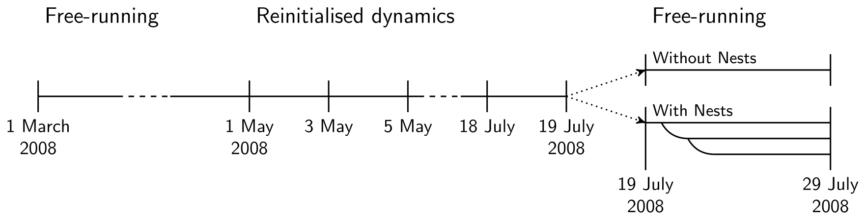
Figure 1 Simulation set-up in this study: a free-running simulation from 1 March until 30 April 2008 is followed by a period until 18 July 2008 where the meteorology is re-initialised every second day. During the mountain wave event until 29 July 2008, two simulations are performed: one global simulation without nests (with 160 km resolution) and one simulation with the nests (with 160, 80 and 40 km resolution) as visualised in Fig. 2 including two-way nesting.

3 Simulation with nests around the Antarctic Peninsula

In 2008, a mountain wave event took place between 19 and 29 July around the Antarctic Peninsula (Noel and Pitts, 2012), which is further investigated in this study. A three-step simulation is conducted; see Fig. 1.

In the first step, the simulation starts on 1 March 2008 with a global resolution of R2B04 (Δx of about 160 km) as a free-running simulation until 1 May 2008. The first of March is chosen because almost no PSCs are formed at this time either in the Northern or in the Southern Hemisphere (Tully et al., 2011). This period is used as a spin-up period for the chemistry until the southern hemispheric polar vortex intensifies (Schoeberl and Newman, 2003), and PSCs formed in 2008 (Tully et al., 2011).

In the second step, the meteorological variables are re-initialised every second day by the reanalysis product of ECMWF, ERA-Interim (Dee et al., 2011), in the period between 1 May and 18 July 2008, but the chemical tracers are free-running. This ensures a comparable evolution of the polar vortex in the model with respect to the reanalysis. This method was already introduced e.g. in Schröter et al. (2018).

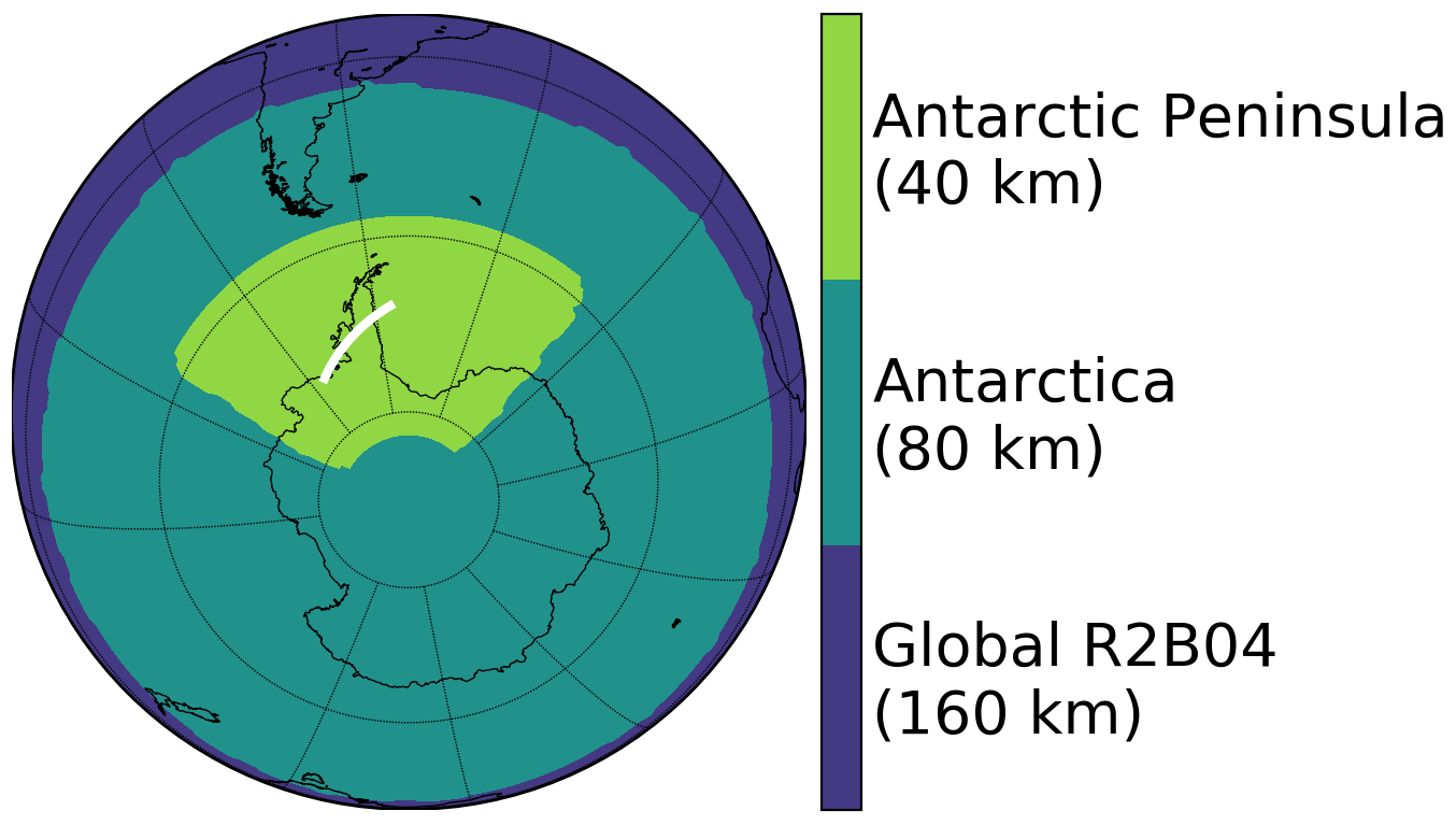
Figure 2 Visualisation of the nested domains used in the simulation with the nests: a global resolution of R2B04 (Δx≈160 km) is used, with the first circular refined grid around the Antarctic continent (R2B05, Δx≈80 km) and a second rectangular refinement around the Antarctic Peninsula (R2B06, Δx≈40 km). The white line shows the location of the cross section analysed in Sect. 5.3.

Table 1 Overview of the simulation set-up for the investigation of the mountain wave event in July 2008. For details see text.

In the third step, we conducted two simulations covering the mountain wave event from 19 to 29 July 2008: one simulation without any nests and one simulation with two-way nesting around the Antarctic continent (R2B05, Δx of about 80 km) and around the Antarctic Peninsula (R2B06, Δx of about 40 km); see Fig. 2 and Table 1. The chemistry – including PSCs, photolysis and transport of tracers – is calculated in all domains. Since we are interested in the interaction between the model domains, we decided to avoid every influence by other models during this part of the simulation, and hence they are free-running. Output in this third step of the simulation is given (1) at the specific Antarctic Peninsula overpasses of AIRS for the Antarctic Peninsula nest and (2) hourly during the whole period of the mountain wave event.

On 1 March 2008, the meteorological variables are initialised with ERA-Interim. The chemical tracers are initialised by an EMAC simulation which included tropospheric as well as stratospheric chemistry similar to Jöckel et al. (2016). Sea surface temperature and sea ice cover are based on monthly varying values of the climatology by Taylor et al. (2000), linearly interpolated to the simulation date. The advective model time step is set to 360 s. Vertically, the same 90 levels are used as in the operational set-up of DWD weather forecasts, covering the altitude range from the surface up to 75 km (see e.g. Weimer et al., 2017, Fig. 1). In the lower stratosphere, the vertical grid spacing increases from 400 m at an altitude of 12 km up to about 1200 m at 30 km.

Table 2 Emission datasets used in this study.

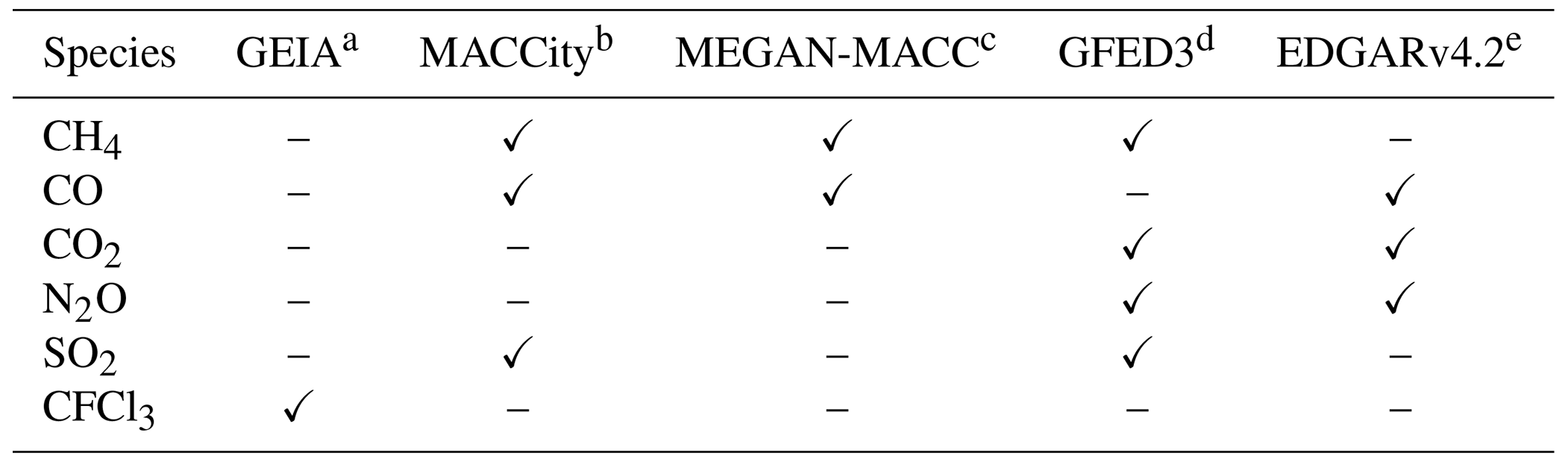
^a Cunnold et al. (1994). ^b van der Werf et al. (2006); Lamarque et al. (2010); Granier et al. (2011); Diehl et al. (2012). ^c Sindelarova et al. (2014). ^d van der Werf et al. (2010). ^e Janssens-Maenhout et al. (2011, 2013).

The emission datasets used in this study are summarised in Table 2. Emissions of CH₄, CO, CO₂, N₂O, SO₂ and CFCl₃ are considered. The Global Emission Inventories Activity (GEIA) dataset for chlorofluorocarbons (CFCs) provided by the Emissions of atmospheric Compounds and Compilation of Ancillary Data database (ECCAD) includes only the year 1986 and should eventually be adapted by the online emission tool by Jähn et al. (2020) for the simulated year. Since the emission rates of CFCl₃ have decreased by more than 40 % since 1986 (Montzka et al., 2018), we neglect the emissions of other CFCs for the less than 1-year simulation. In combination with the emission tool by Jähn et al. (2020) and in the context of the recently found source of CFCs (Montzka et al., 2018; Lickley et al., 2020), further CFCs should be considered in future simulations.

Figure 3 Size distribution of NAT particles used in this study. Based on van den Broek et al. (2004).

NAT PSCs are simulated using a size distribution based on van den Broek et al. (2004), shown in Fig. 3. We prescribe H₂SO₄ in the lower stratosphere (Thomason et al., 2008; SPARC, 2013) in the global domain. In the nested domains, H₂SO₄ runs freely after being initialised by the parent domain.

4 Satellite datasets

4.1 CALIOP

The Cloud-Aerosol Lidar with Orthogonal Polarisation (CALIOP; Pitts et al., 2009, 2018; Höpfner et al., 2009) on board the Cloud-Aerosol Lidar and Infrared Pathfinder Satellite Observation (CALIPSO) was launched on 28 April 2006 (Winker et al., 2007). In 2008, the satellite flew as part of NASA's A-Train constellation in an orbit with 98^∘ inclination at an altitude of 705 km (Stephens et al., 2002; Pitts et al., 2018). Its orbit was sun-synchronous with Equator crossings at about 01:30 and 13:30 LT. It measured down to 82^∘ S with a repeat cycle of 16 d. In February 2018, it was moved to a lower orbit.

CALIOP is a light detecting and ranging (lidar) instrument, set up in nadir geometry. It scans the atmosphere at wavelengths of 532 and 1064 nm with parallel and orthogonal polarisations for the 532 nm channel (Winker et al., 2007). At altitudes from 8.4 to 30 km, the vertical resolution is 180 m or higher. Horizontal averaging of 5 km is applied for the detection of PSCs with CALIOP (Pitts et al., 2018). At the Earth's surface, the light beam has a diameter of about 100 m (Höpfner et al., 2009; Pitts et al., 2018).

For the detection of PSCs, a combination of two values is used (Pitts et al., 2018): (1) the ratio of total and molecular backscatter coefficient R₅₃₂ and (2) the backscatter coefficient at perpendicular polarisation β_⟂, both at a wavelength of 532 nm. Discrimination of the PSC types can be seen in diagrams of R₅₃₂ vs. β_⟂. Different regions in this diagram refer to the different PSC categories: STS, NAT mixtures, enhanced NAT mixtures, ice and wave ice (see Pitts et al., 2018). The thresholds to distinguish PSCs from background noise are calculated as daily median plus 1 absolute standard deviation and depend on potential temperature (${\mathit{\beta }}_{⟂,\mathrm{thres}}$ and R_532,thres). Particles with ${\mathit{\beta }}_{⟂}<{\mathit{\beta }}_{⟂,\mathrm{thres}}$ and $R_{\mathrm{532}}>R_{\mathrm{532},\mathrm{thres}}$ are attributed to the STS category. If ${\mathit{\beta }}_{⟂}>{\mathit{\beta }}_{⟂,\mathrm{thres}}$, non-spherical particles are assumed. Pitts et al. (2018) estimated that 10 % to 15 % of particles classified as NAT mixtures and STS could be misclassified and may lead to enhancements in the respective other class. The boundary between the NAT mixtures and ice (R_NAT|ice) is calculated dynamically depending on the state of dehydration and denitrification (Pitts et al., 2018). The category of enhanced NAT mixtures represents NAT particles nucleated heterogeneously on wave ice PSCs. Both the enhanced NAT mixtures and wave ice categories depend on empirically set thresholds of β_⟂ and R₅₃₂ and therefore are not “all-inclusive” (Pitts et al., 2018). Overall, the classification scheme has been shown to be applicable to ground-based lidars with comparable results (Snels et al., 2019) and has been shown to be in the expected thermodynamic existence regimes (Pitts et al., 2018).

We use the PSC climatology of Pitts et al. (2018), which is the version 2 level 1B data. It is restricted to night-time southern hemispheric data during the mountain wave event (data are available within the time frame we are interested in from 22 to 29 July 2008). We examine the altitude levels between 15 and 30 km where (1) no tropospheric clouds contaminate the results and (2) most of the PSCs can be found (see e.g. Fig. 13 of Pitts et al., 2018). In addition, the dataset includes temperature and pressure data of Modern-Era Retrospective analysis for Research and Applications version 2 (MERRA2; Gelaro et al., 2017), which originally has a horizontal resolution of 0.5^∘ × 0.625^∘, interpolated on the CALIOP paths.

4.2 AIRS

The Atmospheric InfraRed Sounder (AIRS; Aumann et al., 2003; Chahine et al., 2006) is one of the instruments on board the Aqua satellite, which was launched in May 2002 and which is part of the A-Train constellation right ahead of CALIPSO. Thus, its orbit is the same as CALIPSO in 2008 but about 1 to 2 min ahead of CALIPSO¹.

The AIRS instrument is a nadir sounder with across-track scanning capabilities that scans the atmosphere by 90 footprints per scan with a ground coverage of 1780 km and a size of 13.5 × 13.5 km² (nadir) to 41 × 21.4 km² (scan edge) per footprint (e.g. Orr et al., 2015; Hoffmann et al., 2017). It measures the spectrally resolved radiances in wavelengths between 3.74 and 15.4 µm. Brightness temperatures (BTs) in the 15 µm band can be used to derive information about gravity waves in the lower polar stratosphere (Hoffmann et al., 2017). In this study we use a data product averaging over 21 channels around 15 µm to improve the signal-to-noise ratio (Hoffmann et al., 2017). The temperature weighting function in this band peaks at an altitude of around 23 km with a full width at half maximum of 15 km and with information from the altitude range between 17 and 32 km. Therefore, it is well suited to derive information about gravity waves in the altitude region where PSCs are expected to exist.

This band is used to examine the mountain wave event at the Antarctic Peninsula mentioned above. The same algorithm as in previous studies is used to compare the model data with specific Antarctic Peninsula overpasses of AIRS (Hoffmann and Alexander, 2010; Hoffmann et al., 2016, 2017). In particular, the ICON-ART data are resampled on the AIRS measurement grid, and a radiative transfer model is used to simulate AIRS measurements based on the ICON-ART data to allow for a direct comparison with the real observations.

5 Mountain-wave-induced PSCs with ICON-ART

Here, we investigate a mountain wave event during July 2008 with ICON-ART in a configuration with interactive chemistry and local grid refinement around the Antarctic Peninsula. This section comprises an evaluation of the dynamical structure of the mountain wave with AIRS (Sect. 5.1) and comparisons of the model results with CALIOP measurements (Sect. 5.2). In addition, it discusses the impact of the direct simulation of mountain-wave-induced PSCs on the polar ozone chemistry (Sect. 5.3).

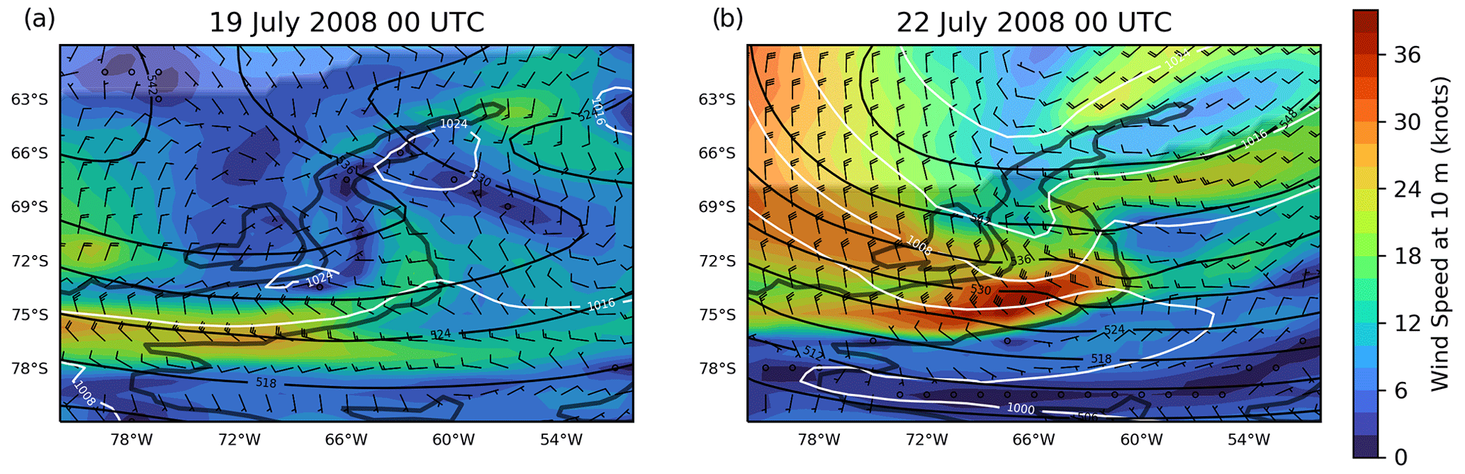
Figure 4 Meteorological situation at the Antarctic Peninsula for (a) 19 and (b) 22 July 2008 at 00:00 UTC from ERA-Interim. The colours and the wind barbs depict the surface wind in knots. The white lines correspond to the mean sea level pressure in hectopascals. The black lines are geopotential heights at 500 hPa in geopotential decametres. The shaded regions show the air masses within the polar vortex, determined according to Nash et al. (1996) on θ=475 K. Panels covering the whole period of the mountain wave event can be found in the Supplement.

5.1 Near-surface meteorological conditions and stratospheric dynamical structure of the mountain wave

The evolution of the ozone loss and the Antarctic polar vortex in 2008 was comparable to the previous years although the so-called ozone hole lasted rather long into December (Tully et al., 2011). It was a year with increased gravity wave activity at the Antarctic Peninsula (Hoffmann et al., 2016). We chose a gravity wave event lasting 10 d from 19 until 29 July 2008 with lowest temperatures during the whole winter season (Noel and Pitts, 2012). By end of July 2008, the polar vortex was close to its maximum extension, whereas the stratospheric ozone concentration started to decrease (Tully et al., 2011).

Figure 4 summarises the large-scale meteorological conditions around the peninsula, based on the ERA-Interim reanalysis. As indicated e.g. by Alexander and Teitelbaum (2007), the ability of ERA-Interim to capture mesoscale mountain wave events is limited. Therefore, we use the reanalysis to show the meteorological background conditions and will evaluate the lower-stratospheric temperature perturbations with AIRS later in this section. Figure 4 shows several variables at the beginning of the mountain wave event on 19 July 2008 (panel a) and around its peak dynamics on 22 July 2008 (panel b). Panels covering the whole event can be found in the Supplement (Fig. S1).

The Antarctic Peninsula was located at the vortex edge during the whole mountain wave event, as depicted by the shaded regions in the panels and determined by the method by Nash et al. (1996). Starting from 19 July 2008, an approaching high-pressure system led to an increase of the mean sea level pressure gradient (white lines) at the Antarctic Peninsula with a corresponding increase of easterly winds at the mountain range (wind barbs and colour-coded). The gradient on the geopotential height at 500 hPa (black lines) was also increased, showing the large-scale easterly flow at this altitude on 22 July.

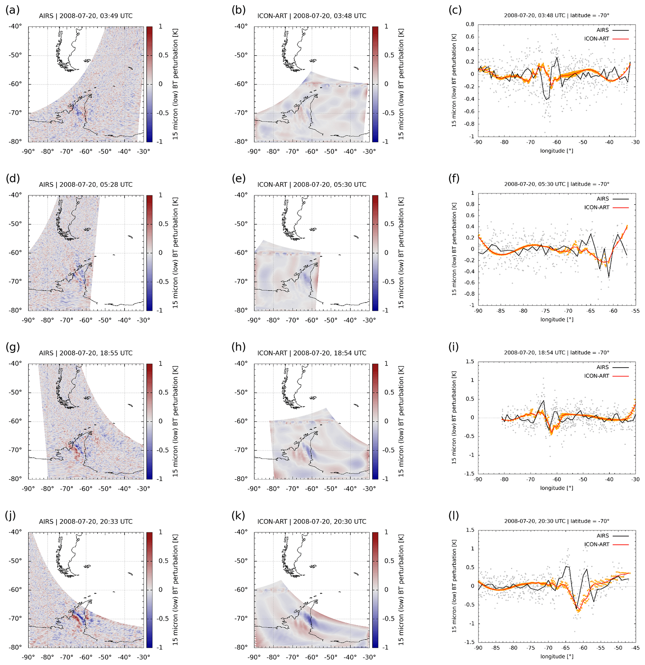
Figure 5 Comparison of AIRS and ICON-ART brightness temperature (BT) perturbations at wavelengths of 15 µm for all Antarctic Peninsula overpasses of AIRS during 20 July 2008. The first column shows the BT perturbation observed by AIRS, and the second column the simulated perturbation based on ICON-ART in the Antarctic Peninsula nest. The third column shows the perturbation for AIRS (black) and ICON-ART (orange) at a latitude of 70^∘ S. The rows show different overpasses at (a–c) 03:49 UTC, (d–f) 05:28 UTC, (g–i) 18:55 UTC and (j–l) 20:33 UTC.

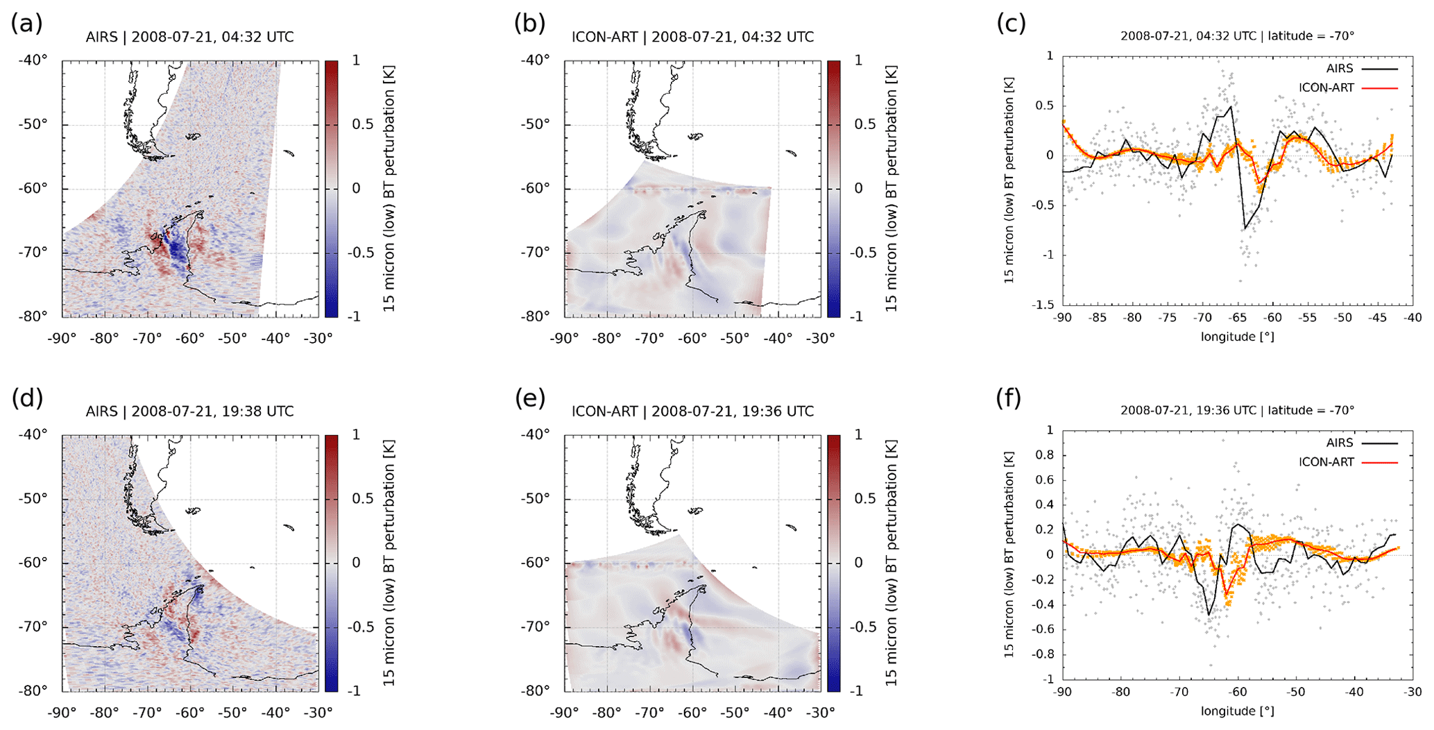
Figure 6 Same as Fig. 5 but for 21 July 2008. The rows show different overpasses at (a–c) 04:32 UTC and (d–f) 19:38 UTC.

These conditions led to a mountain wave event lasting for 10 d, which is now compared to AIRS measurements. For this, temperature and pressure of ICON-ART in the Antarctic Peninsula nest are saved at the time step closest to each of the AIRS overpasses during 20 and 21 July 2008. These data are then convolved with the same temperature weighting functions that apply for the AIRS observations (see e.g. Hoffmann et al., 2017). The same methodology was applied to model simulations by Orr et al. (2015). The resulting BT perturbations can be found in Fig. 5 on 20 July and in Fig. 6 on 21 July 2008 for AIRS and ICON-ART.

Horizontal structures of the BT perturbations are shown in the first and second columns for AIRS and ICON-ART, respectively. Largest perturbations are present directly above the Antarctic Peninsula for both AIRS and ICON-ART, which demonstrates that the perturbations originate from mountain waves propagating into the lower stratosphere. In addition, the mountain wave has an angle with respect to the Antarctic Peninsula mountains of about 45^∘, represented in both AIRS and ICON-ART. The horizontal wavelength of the simulated mountain wave is in the order of 300 km, which is a medium–large wavelength compared to other events (see e.g. Alexander and Teitelbaum, 2007; Plougonven et al., 2008; Hoffmann et al., 2014). Therefore, the ICON-ART simulation with lower-stratospheric vertical resolution in the order of 500 m and horizontal resolution of 40 km in the Antarctic Peninsula nest can capture the main features of the mountain wave.

Fine structures such as in panel j of Fig. 5 cannot be simulated in this simulation set-up of ICON-ART (e.g. panel k) since the resolution of 40 km is still too coarse to predict them, which was already indicated by the comparison to CALIOP. This might be a resolution issue which would perhaps be improved by going to higher grid spacings, as shown by Orr et al. (2015). The chemistry non-linearly depends on temperature, which means that small temperature variations could have a measurable effect on the chemistry (e.g. Murphy and Ravishankara, 1994). As pointed out previously, the microphysics of PSCs are one example for this. If the amplitude is underestimated, like in Fig. 5b and c, a more highly resolved model would most probably generate more ice PSCs, thus improving the CALIOP comparison at the lowest temperatures; cf. e.g. Figs. 5 to 7 of Orr et al. (2020), who used a higher-resolution simulation to parameterise mountain-wave-induced PSCs.

These results are also stressed by the comparison of the perturbations at the latitude of 70^∘ S that are shown in the third column of Figs. 5 and 6. The largest BT perturbations can be found at the longitude of the Antarctic Peninsula in all the panels. Some fine structures are missing in ICON-ART. For instance, at some overpasses the amplitude of the wave is underestimated compared to AIRS (e.g. panel c of Fig. 6). An analogous study by Orr et al. (2015) using a 4 km resolution seems to suggest a better match between model and observations. At other overpasses, the phase of the wave is shifted with respect to AIRS, such as in panel c of Fig. 5 and panel f of Fig. 6. This is most probably a result of the free-running simulation where the wave cannot be expected to be located at exactly the same location as in the measurements.

In total, the comparison with AIRS showed that, apart from some missing fine structures, the mountain wave event taking place in the end of July 2008 can be represented with the resolution of 40 km in comparison with AIRS. In the following, we will analyse how this directly simulated mountain wave event impacts the dynamics in the coarser-resolution domains in ICON-ART.

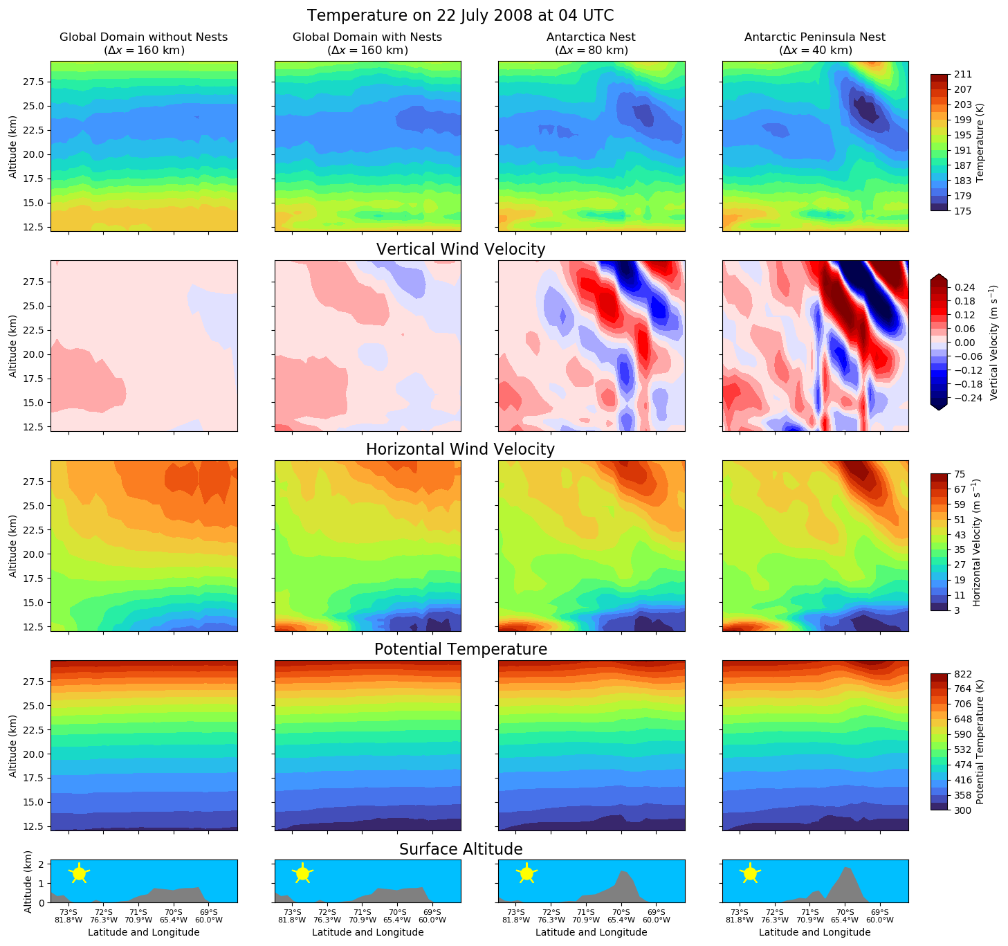
Figure 7 Cross sections on 22 July 2008 at 04:00 UTC along the white line in Fig. 2. Each row represents a different variable in the model. The bottom row shows the surface altitude with the Antarctic Peninsula at around 65^∘ W. The columns represent the different simulations and domains: the first column is the simulation without nests (Δx≈160 km); the second one is the global domain (Δx≈160 km) including two-way nesting; and the two right columns represent the Antarctica (Δx≈80 km) and Antarctic Peninsula nests (Δx≈40 km), respectively. The dynamical variables temperature, vertical wind velocity, horizontal wind velocity and potential temperature are shown in this figure.

Figure 7 shows cross sections of the mountain wave dynamics along the line shown in Fig. 2 for the example of 22 July 2008 at 04:00 UTC in the altitude range between 12 and 30 km. The model data are interpolated to the path by an inverse distance method including the three neighbouring grid points. The left column shows the simulation without nests, whereas the three other columns illustrate the dynamics in the different domains shown in Fig. 2 of the simulation with the nests.

The bottom row of Fig. 7 shows the resolution of the Antarctic Peninsula in the different domains. As can be seen, the higher the horizontal resolution, the better the Antarctic Peninsula can be represented as mountain range. Thus, this indicates that the interaction between the flow and the detailed orography in the Antarctic Peninsula nest is improved with respect to the global resolution of 160 km.

This is reflected in the variables shown in Fig. 7. Temperatures close to 175 K only occur in the Antarctic Peninsula nest with a 40 km resolution in the lee of the mountain. The temperature in the Antarctic Peninsula nest also shows the characteristic high- and low-temperature patterns as calculated in theory (e.g. Queney, 1947; Smith, 1989) and seen in measurements (e.g. Wright et al., 2017). As already indicated by Figs. 5 and 6, the temperature perturbation in the order of 10 K compares well to the AIRS measurements and is also consistent with previous studies of mountain waves (Meilinger et al., 1995; Carslaw et al., 1998a; Eckermann et al., 2009).

The relatively large temperature gradients in the Antarctic Peninsula nest are also in agreement with gradients in the wind velocities, which are shown in the second and third row of Fig. 7. In the lee of the Antarctic Peninsula, the vertical wind velocity changes signs at altitudes where the temperature increases or decreases and has maximum values above 0.3 m s⁻¹. Largest horizontal wind velocities in the order of 75 m s⁻¹ occur at altitudes above 27 km.

The mountains also cause perturbations in the potential temperature (fourth row in Fig. 7) in the lee. If diabatic processes are negligible, the flow follows the contours of potential temperature, which will be shown in the PSC precursors in Sect. 5.3.2.

Up to now, it was only demonstrated that this mountain wave event can be directly simulated in the Antarctic Peninsula nest (right column), compares well to measurements and is consistent with the theory of mountain waves (Queney, 1947; Smith, 1989). In addition, Fig. 7 also shows the impact of the two-way nesting in ICON-ART. The nest around Antarctica with a resolution of about 80 km (third column) interacts with both nests and shows the transition between these resolutions. The mountain wave at the Antarctic Peninsula cannot be represented adequately at the resolution of 160 km in the simulation without the nests (left column in Fig. 7). The characteristic wave patterns do not occur in this simulation. In contrast to this, the global domain in the simulation with the nests (second column in Fig. 7) shows a decrease in temperature of about 2 K in the lee of the mountains. This is a result of the two-way nesting and the lower temperature due to the directly simulated mountain wave in the Antarctic Peninsula nest. The amplitude is lower than it is expected by mountain waves, but the effect of the mountain wave is still remarkable, even in the global grid of 160 km resolution.

This is also visible in the other variables of Fig. 7. Especially for the vertical wind velocity (second row), one can see that wave-like structures occur in the global domain where they cannot be represented without the nests. Therefore, we can expect that mountain-wave-induced PSCs can also be represented at this relatively low global resolution because they are directly simulated in the locally refined regions. In the following section, we will compare PSCs to CALIOP measurements in the Antarctic Peninsula nest before we analyse the impact of further model variables on the chemistry.

5.2 Comparison of simulated PSCs with CALIOP measurements

For a comparison with CALIOP, the ICON-ART PSC volume concentrations are interpolated (1) horizontally by an inverse distance method, (2) linearly in time and (3) linearly in geometric altitude to all CALIOP paths from 22 to 29 July 2008 where CALIOP's orbit was within the region of the Antarctic Peninsula nest. Details about the interpolation can be found in Weimer (2019, Sect. 4.7.4).

As pointed out by previous studies, an adequate comparison of CALIOP with model data can only be set up if the model data are transferred into the optical space measured by CALIOP at 532 nm. We apply the method by Engel et al. (2013), Tritscher et al. (2019) and Steiner et al. (2021). It is based on T-matrix and Mie calculations (e.g. Mishchenko et al., 1996) with particle number densities and particle radii of the PSC types as input. The external PSC mixtures of ICON-ART are combined to optical properties (R₅₃₂ and β_⟂) for each grid point. In accordance with Tritscher et al. (2019) and Steiner et al. (2021) we use aspect ratios of ice and NAT of 0.9 and refractive indices of 1.44 for STS (Krieger et al., 2000), 1.31 for ice and 1.48 for NAT (Middlebrook et al., 1994).

The three thresholds to determine the boundaries between the PSC categories, as mentioned in Sect. 4.1, are taken from the measurement data and averaged daily for each CALIOP height level (${\stackrel{\mathrm{‾}}{\mathit{\beta }}}_{⟂,\mathrm{thres}}$, ${\stackrel{\mathrm{‾}}{R}}_{\mathrm{532},\mathrm{thres}}$ and ${\stackrel{\mathrm{‾}}{R}}_{\mathrm{NAT}|\mathrm{ice}}$) (Tritscher et al., 2019; Steiner et al., 2021). As pointed out by Engel et al. (2013), it is important to account for the measurement uncertainties σ_R and ${\mathit{\sigma }}_{\mathit{\beta },⟂}$ to compare the simulated R₅₃₂ and β_⟂ with CALIOP. These uncertainties are calculated according to Eqs. (5) and (6) of Tritscher et al. (2019), respectively. The simulated R₅₃₂ and β_⟂ are scaled by a normal distribution with mean at the simulated value and standard deviation as the respective σ. To summarise, the condition to determine if a PSC is detected is then

$$\begin{array}{}\text{(1)}& {\mathit{\beta }}_{\mathrm{scal}}>{\stackrel{\mathrm{‾}}{\mathit{\beta }}}_{⟂,\mathrm{thres}}+{\mathit{\sigma }}_{\mathit{\beta },⟂},{\mathit{\beta }}_{\mathrm{scal}}\sim \mathcal{N}({\mathit{\beta }}_{⟂},{\mathit{\sigma }}_{\mathit{\beta },⟂}^{\mathrm{2}})\end{array}$$

or

$$\begin{array}{}\text{(2)}& R_{\mathrm{532},\mathrm{scal}}>{\stackrel{\mathrm{‾}}{R}}_{\mathrm{532},\mathrm{thres}}+{\mathit{\sigma }}_R,R_{\mathrm{532},\mathrm{scal}}\sim \mathcal{N}\left(R_{\mathrm{532}},{\mathit{\sigma }}_R^{\mathrm{2}}\right).\end{array}$$

Since the ICON-ART simulations are free-running, we cannot expect the PSCs to occur at exactly the same locations as in the measurements. Therefore, we compare the evolution of PSCs with respect to the temperature in both CALIOP and ICON-ART, which is a crucial parameter in the formation of PSCs (e.g. Solomon, 1999). We count the occurrence of the different PSC categories by the method described above in temperature bins and compare them between ICON-ART and CALIOP. The “no” PSC category is neglected in this comparison to emphasise the occurrence of PSCs in the temperature bins. The data are restricted to the region of the Antarctic Peninsula nest resulting in a total number of about 1 million grid points with PSCs for CALIOP and about 0.5 million grid points with PSCs in ICON-ART. This large difference could be either a result of horizontally shifted PSCs, especially in the later part of the free-running simulation, or a problem with the constant number concentrations used in the model. It should be further analysed in the future.

Figure 8 Statistical analysis of PSC occurrence for (a) the ICON-ART simulation without nests, (b) the ICON-ART simulation with nests in the Antarctic Peninsula nest and (c) CALIOP measurements. The data are restricted to the region of the Antarctic Peninsula nest for all panels to get comparable results. The ICON-ART data are interpolated to the CALIOP paths in the altitude range from 15 to 30 km in the nest in the time range between 22 and 29 July 2008 where CALIOP data are available. The colours correspond to the numbers in the circles and show the fraction of the PSC category that is present in the temperature bins with a width of 3.5 K. The sizes of the circles correspond to the total number of grid points with PSCs in the temperature bins relative to the maximum in each panel, also denoted on the right-hand side of the panels as N_PSC, following the nomenclature by Spang et al. (2016). The “k” behind the numbers abbreviates thousand; i.e. 179.7 k = 179 700 grid points with PSCs. The temperature data for CALIOP originate from MERRA2, which is part of the CALIOP product.

Figure 8 shows the relative number of grid points (in per cent) on the CALIOP paths where the different PSC categories occur. The size of the circles corresponds to the total number of grid points with PSCs, and the colour of the circles shows the relative number of this PSC category occurrence in the respective temperature bin. The panels show the PSC occurrence (a) in the simulation without the nests, (b) in the Antarctic Peninsula nest and (c) in the CALIOP measurements. For ICON-ART (panels a and b), the modelled temperatures are used directly. The temperature for CALIOP (panel c) is interpolated from MERRA2 and provided as part of the original dataset (Pitts et al., 2018).

As can be seen, the relative distribution of grid points with PSCs coincides in all panels down to a temperature of about 180 K. Temperatures lower than that, however, are underrepresented in the simulation without the nest, compared to CALIOP. This is expected from Fig. 7 since temperatures are higher than 180 K in the simulation without nests in the lee of the mountains. In addition, the simulation without nests overestimates the fraction of the ice category at temperatures lower than 183 K compared to CALIOP.

Both deficiencies are improved in the Antarctic Peninsula nest with a resolution of 40 km (panel b). PSCs in the ice category occur with a similar fraction like in CALIOP in the 181 K bin, and the relative number of grid points with PSCs in the lowest temperature bin coincides with the measurements. The fractions of the NAT mixtures and enhanced NAT categories are also comparable to CALIOP over the whole range of temperatures. For medium temperatures (188 and 184.5 K) the fraction of the STS category is slightly overestimated compared to CALIOP. A reason for this could be missing fine structures in the gravity wave, as already indicated by Figs. 5 and 6. The fraction of the ice category is 9 % larger in the lowest temperature bin than in CALIOP.

Although Fig. 7 suggests that main parts of the mountain wave can be captured in the Antarctic Peninsula nest, no PSCs in the “wave ice” category are simulated by ICON-ART. As mentioned in Sect. 2, the ice particle number concentration is essentially set to the constant value of 0.25 cm⁻³ in the stratosphere. The ice number concentration in mountain waves can increase to values of a few cubic centimetres and then lead to larger backscatter ratios (e.g. Engel et al., 2013). Therefore, this too-low ice number concentration could explain why the backscatter ratio for determining the PSC categories does not get as large as 50, which is needed for the wave ice category (Pitts et al., 2018). On the other hand, as mentioned in Sect. 4.1, the wave ice category is based on an empirical threshold of R₅₃₂>50, so that parts of the wave ice clouds could also be attributed to the ice category (Pitts et al., 2018).

Comparing the three panels of Fig. 8, there seems to be a resolution-dependent shift of overestimated fraction in the ice category. At the resolution of 160 km, the overestimation starts at the 181 K bin; for 40 km it begins at 177.5 K. Thus, this figure gives first hints that using an even higher resolution could improve the comparison of the PSC distributions at low temperatures with CALIOP since the amplitude of the mountain wave may be better represented, as already mentioned in the comparison with AIRS in Sect. 5.1. Similar findings by Orr et al. (2020) corroborate this. It is also consistent with other previous studies with mesoscale models that used a higher resolution to study mountain waves (e.g. Noel and Pitts, 2012) and should be one focus of future simulations.

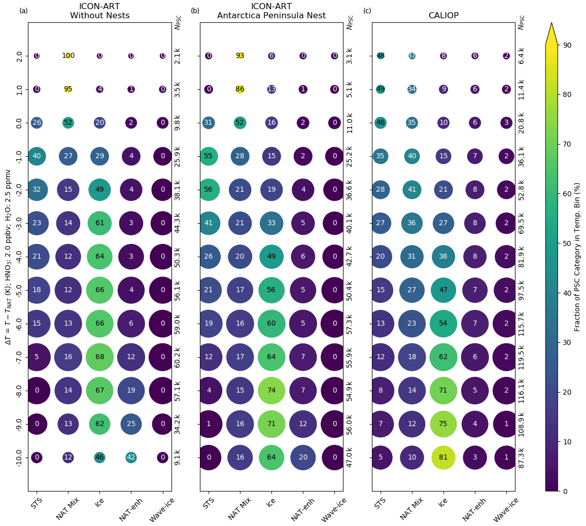
Figure 9 Same as Fig. 8 but relative to T_NAT. Here, a common T_NAT for both ICON-ART and CALIOP y axes is derived from Hanson and Mauersberger (1988) with input of $X_{{\mathrm{H}}_{\mathrm{2}}\mathrm{O}}=\mathrm{2.5}\mathrm{ppmv}$ and $X_{{\mathrm{HNO}}_{\mathrm{3}}}=\mathrm{2}\mathrm{ppbv}$ based on Tritscher et al. (2019). The data are binned in terms of temperature difference with a bin width of 1 K.

Figure 10 Same as Fig. 8 but relative to T_ice. Here, a common T_ice for ICON-ART and CALIOP y axes is derived from Marti and Mauersberger (1993) with input of $X_{{\mathrm{H}}_{\mathrm{2}}\mathrm{O}}=\mathrm{2.5}\mathrm{ppmv}$ based on Tritscher et al. (2019). The data are binned in terms of temperature difference with a bin width of 1 K.

This shift in the fraction of the ice category is emphasised in Figs. 9 and 10. They show the evolution of the PSC categories relative to the NAT and ice formation temperatures, T_NAT and T_ice. We calculated these temperatures with $X_{{\mathrm{H}}_{\mathrm{2}}\mathrm{O}}=\mathrm{2.5}\mathrm{ppmv}$ and $X_{{\mathrm{HNO}}_{\mathrm{3}}}=\mathrm{2}\mathrm{ppbv}$ based on the formulas by Hanson and Mauersberger (1988) and Marti and Mauersberger (1993), respectively, to get a comparable pressure-dependent reference temperature for both the model and the measurements. These constant volume mixing ratios are used only to calculate the PSC existence temperatures. They are based on satellite measurements shown by Tritscher et al. (2019) for late July, accounting for denitrification and dehydration.

As can be seen in Fig. 9, the number of grid points with PSCs grows when the temperature gets lower than T_NAT in all three panels. Similar patterns to those in Fig. 8 can be seen: overestimation of the STS category at temperatures around 1 to 3 K lower than T_NAT in the Antarctic Peninsula nest and differences in the ice category. In the case of the simulation without nests, the fractions of ice are larger than in CALIOP for ΔT_NAT<0 K. In the Antarctic Peninsula nest, this overestimation can be seen at temperatures $\mathrm{\Delta }{T}_{\mathrm{NAT}}<-\mathrm{2}\mathrm{K}$. These deficiencies should be analysed in future simulations.

The comparison with respect to T_ice in Fig. 10 emphasises the previous findings. In the simulation without the nests, temperatures lower than $\mathrm{\Delta }{T}_{\mathrm{ice}}=-\mathrm{3}\mathrm{K}$ are underrepresented compared to CALIOP. The fraction of the ice category peaks with 69 % at $\mathrm{\Delta }{T}_{\mathrm{ice}}=-\mathrm{1}\mathrm{K}$. The resolution of 40 km in the Antarctic Peninsula nest is able to reproduce the general evolution of PSCs for $\mathrm{\Delta }{T}_{\mathrm{ice}}<-\mathrm{3}\mathrm{K}$, but the fraction peaks with 74 % at $\mathrm{\Delta }T\mathrm{ice}=-\mathrm{2}\mathrm{K}$. In contrast, the CALIOP measurements suggest that the fraction of the ice category should be larger for $\mathrm{\Delta }{T}_{\mathrm{ice}}<-\mathrm{2}\mathrm{K}$. An even higher resolution might help to reflect ice PSCs at these temperatures, as discussed in the comparison with AIRS (compare also with Orr et al., 2020).

In total, this section has demonstrated that the PSC scheme in ICON-ART is able to generate PSCs similar to CALIOP. The peak fraction of the ice category seems to move to lower temperatures if the resolution is increased, which might indicate that an even higher resolution is needed to capture the ice formation at the lowest temperatures (cf. Orr et al., 2020). On the other hand, this analysis demonstrated that the evolution of the PSCs is clearly improved in the Antarctic Peninsula nest with respect to CALIOP. Some differences in the STS category with respect to CALIOP also indicate that some fine structures of the mountain wave are missing, consistent with the previous findings in the comparison with AIRS.

5.3 Impact of mountain-wave-induced PSCs on the chemistry

In the previous sections, it was demonstrated that both the PSC formation and the formation of the mountain wave are in relatively good agreement with measurements considering the limits in measurements and simulation set-up. In this section, we investigate the impact of directly simulated mountain-wave-induced PSCs on the interactively calculated chemistry in ICON-ART. The analysis is focused on the mountain wave event at its peak dynamics on 22 July 2008 (see Figs. 4 and S1).

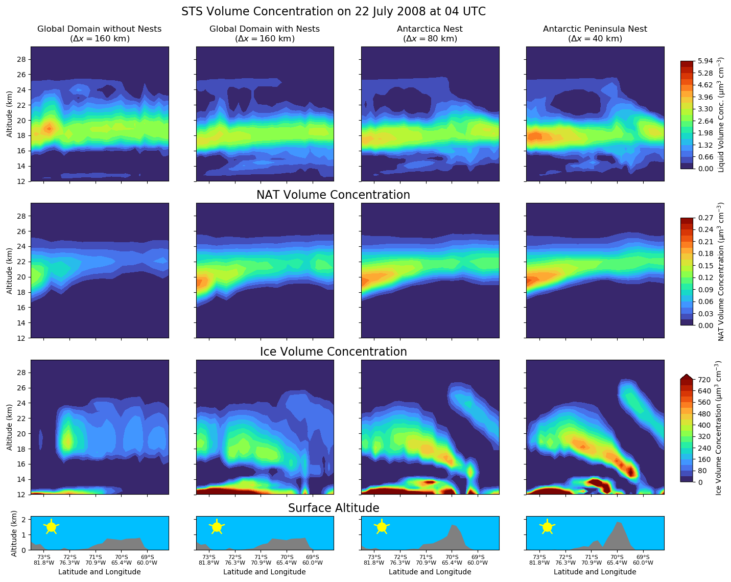
Figure 11 Same as Fig. 7 but for the volume concentrations of the different PSCs: liquid aerosol, NAT and ice. Please note the different colour bars.

5.3.1 The formation of PSCs in the mountain wave

Figure 11 demonstrates that the ICON-ART model has the potential to close the gap between direct simulations of mountain-wave-induced PSCs and their treatment at relatively coarse global resolutions. The volume concentration of liquid particles (first row) in the global domain with nests is influenced by the mountain wave, especially at altitudes higher than 20 km, where particle volume concentrations close to zero occur in the global domain which do not exist without the nesting technique. The influence of the mountain wave on liquid aerosol is amplified within the nests. The liquid particles are assumed to freeze at temperatures 3 K below the frost point (Carslaw et al., 1995; Koop et al., 2000). Thus, liquid particles are only computed for higher temperatures so that they are formed in the mountain wave where the temperature is higher than this threshold.

STS and NAT compete with each other in taking up HNO₃. This is why in this case study distinct layers exist: NAT PSCs at altitudes higher than 20 km and STS PSCs at lower altitudes where H₂SO₄ is also enhanced; see Sect. 5.3.2. The NAT volume concentrations are increased in the Antarctic Peninsula nest (second row, right column), which is why they are also increased in the global domain comparing the simulations with and without nests.

In contrast to the literature (e.g. Carslaw et al., 1999; Svendsen et al., 2005), the NAT volume concentration decreases when the air masses approach the mountain wave. Since the NAT size bins are advected with the general air masses, the wave-like patterns occur in both nests. As a result of the operator splitting used in ICON-ART, the largest fraction of gaseous H₂O leads to ice formation at temperatures lower than about 180 K and is not available for NAT PSCs and liquid particles in the mountain wave anymore. Therefore, the largest signal of mountain-wave-induced PSCs can be found in ice PSCs in Fig. 11. This is an issue of further investigation in the future. In addition, NAT PSCs are formed by freezing STS particles in the mountain wave, as shown e.g. by Bertram et al. (2000) and Salcedo et al. (2001). This is not integrated in the model yet and should be considered in the future.

The best example of the formation of mountain-wave-induced PSCs is ice PSCs (third row in Fig. 11). In the lee of the Antarctic Peninsula ice PSCs occur with volume concentrations as large as 700 µm³ cm⁻³. These relatively high values might be overestimated because of the assumptions in the hydrometeor microphysics of the meteorological model (Doms et al., 2011). As discussed above, the ice number concentration is too low for mountain wave conditions compared to measurements. A more realistic number concentration would lead to smaller ice particles and could reduce the ice volume concentration to more realistic values.

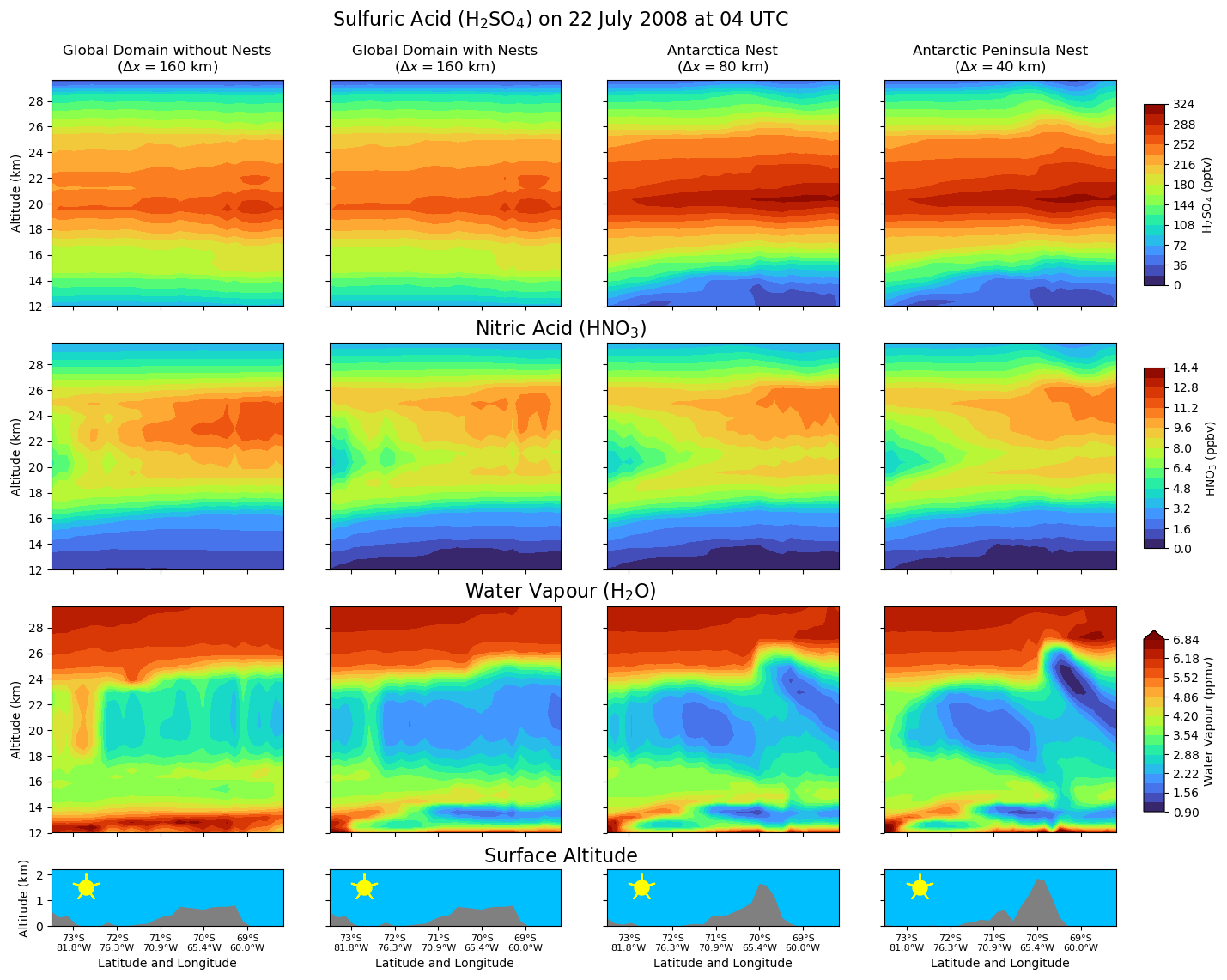
Figure 12 Same as Fig. 7 but for the tracers that are relevant for the formation of PSCs: H₂SO₄, HNO₃ and H₂O. Please note the different colour bars.

On the other hand, the ice PSCs are clearly connected to the regions where temperature is decreased and show similar wave-like patterns to the temperature. These increased volume concentrations are also present in the global domain where wave-like patterns can be simulated with the nests, in contrast to the simulation without the nests, where these structures do not exist.

Therefore, this figure shows that mountain-wave-induced PSCs can be directly simulated with ICON-ART for this specific event. Their effect can also be treated in the global domain where mountain-wave-induced PSCs cannot be represented without the nests. The PSCs also interact with the gaseous species which are analysed in the next section.

5.3.2 Influence of the mountain wave on PSC precursors

As mentioned above, long-lived tracers closely follow the potential temperature. Therefore, the wave perturbations in potential temperature can be seen in all tracers shown in Fig. 12 in the lee of the mountain for the simulation with the nests. The wave-like structures in sulfuric acid (H₂SO₄, first row), nitric acid (HNO₃, second row) and water vapour (H₂O, third row) correspond to the structures seen in the potential temperature (see Fig. 7).

H₂SO₄ is prescribed by a climatology in the global domain but free-running in the nests and only shows a minor signal of the two-way nesting. Due to the missing sink of H₂SO₄ by sedimentation of aerosols (see Sect. 3) and advection processes, the mixing ratio accumulates in the nested domains (two right columns).

HNO₃, shown in the second row of Fig. 12, is taken up by STS and NAT PSCs so that it is lower in the simulation with nests than in the simulation without the nests. This not only is shown in both nested domains but can also be returned to the global domain as a result of the two-way nesting.

Figure 13 Same as Fig. 7 but for the chlorine species, HCl and ClONO₂, and the sum of all other (active) chlorine-containing species (ClO_x). The colour bars are equal in this figure.

This property especially occurs for H₂O. In the lee at altitudes between 22 and 25 km, temperatures lower than about 179 K lead to volume mixing ratios lower than 1 ppmv that are connected with the uptake in ice PSCs (cf. Fig. 11). The resolution of 80 km in the Antarctica nest (third column) misses a larger part of the wave, but the wave-like pattern can still be seen for H₂O. It cannot be represented in the simulation without the nests (left column) where the H₂O volume mixing ratio does not decrease to values lower than 2.5 ppmv. In the global domain of the simulation with the nests, however, values as low as 2 ppmv occur in the lee of the mountain as a result of the two-way nesting.

5.3.3 Impact of mountain-wave-induced polar stratospheric clouds on chlorine activation

Both the directly simulated mountain-wave-induced PSCs and the lower wave-driven temperature in the simulation with the nests also affect other species. The chlorine species are summarised in Fig. 13 in the same way as in the previous figures. The reservoir species hydrochloric acid (HCl, first row) and chlorine nitrate (ClONO₂, second row) are shown together with the active chlorine species (third row), summarised as ClO_x:

$$\begin{array}{}\text{(3)}& \begin{array}{rl}& X_{{\mathrm{ClO}}_x}=X_{{\mathrm{ClNO}}_{\mathrm{2}}}+\mathrm{2}{X}_{{\mathrm{Cl}}_{\mathrm{2}}{\mathrm{O}}_{\mathrm{2}}}+X_{\mathrm{OClO}}+\mathrm{2}{X}_{{\mathrm{Cl}}_{\mathrm{2}}}\\ & +X_{\mathrm{BrCl}}+X_{\mathrm{HOCl}}+X_{\mathrm{Cl}}+X_{\mathrm{ClO}}.\end{array}\end{array}$$

During July, which is a relatively late stage of the southern polar winter, most of the chlorine species in the altitude range between 15 and 25 km have been already activated (cf. Tully et al., 2011). The broad band of volume mixing ratios of ClO_x with values up to about 2.2 ppbv that are present in all panels of the third row suggests this. Therefore, additional chlorine activation can only be expected at altitude regions above 25 km. In the previous sections, it was shown that the directly simulated mountain-wave-induced ice PSCs reach altitudes of about 26 km (see Fig. 11).

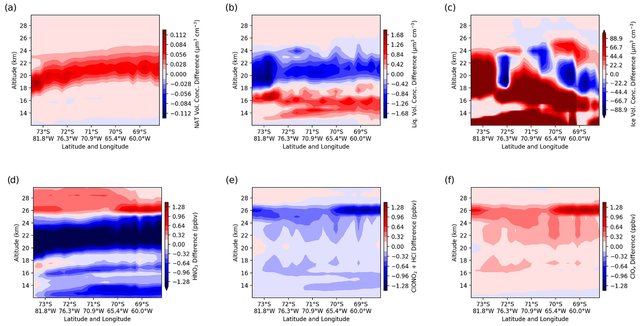
Figure 14 Difference in global domain with and without nest around the Antarctic Peninsula along the cross section shown in Fig. 2 at the same date (22 July 2008, 04:00 UTC) and using the same algorithm as in the previous figures. The shown variables are differences in (a–c) the NAT, liquid and ice volume concentrations, respectively; (d) the HNO₃ volume mixing ratio; (e) the volume mixing ratio of the reservoir species ClONO₂ and HCl; and (f) the ClO_x as defined in Eq. (3). Minimum values of HNO₃ are around 2.3 ppbv.

Low temperature and mountain-wave-induced PSCs lead to increased chlorine activation in the lee of the Antarctic Peninsula that is not present in the simulation without the nests. At altitudes around 26 km, the additional ice PSCs activate both ClONO₂ and HCl in the lee of the mountains. This is shown by values of the reservoir species around zero and values of ClO_x up to 3 ppbv in this region that cannot be simulated without the nests. These increased ClO_x mixing ratios also have an effect on ozone in the model, which will be shown in the next section.

5.3.4 Impact of mountain-wave-induced polar stratospheric clouds on ozone

A summary of the impact of the two-way nesting on mountain-wave-induced PSCs and the chemistry can be found in Fig. 14. It shows the differences of the two global domains with and without the nests for various variables of the previous sections. Panel a shows the difference in the NAT volume concentration, and it can be seen that more NAT particles are produced in the simulation with the nests as a result of the two-way nesting. These enhanced NAT volume concentrations lead to (1) a decreased volume concentration of liquid particles (panel b) as a result of the operator splitting used and (2) decreased values of HNO₃ (panel d) with differences lower than −1.4 ppbv in this region since HNO₃ is taken up by NAT particles. In regions where no additional NAT particles exist, the liquid volume concentration is enhanced due to the two-way nesting (panel b). In the ice volume concentration in panel c, the wave-like structure is clearly present.

The mountain-wave-induced (ice) PSCs and low temperatures lead to additional chlorine activation, in this example at an altitude of about 26 km. The negative difference in the sum of ClONO₂ and HCl (panel e) is closely connected to the positive differences in ClO_x in the lee of the mountain (panel f). HNO₃ is also a product of heterogeneous reactions on the surface of PSCs and therefore is enhanced in this region with respect to the simulation without the nests (panel d).

Due to transport of the activated chlorine species and PSCs, ozone depletion might take place downstream of the Antarctic Peninsula (e.g. Höpfner et al., 2006b). Therefore, ozone is affected by the mountain wave event (1) far in the lee of the mountain and (2) later in the year. This is why the time series of the southern hemispheric mean total ozone column for the whole third period of the simulation is shown in Fig. 15. The ozone columns are averaged for latitudes south of 60^∘ S. Two lines are shown in panel a: the solid line is the mean total ozone column in the global domain of the simulation with the nests, whereas the dashed line illustrates the simulation without the nests.

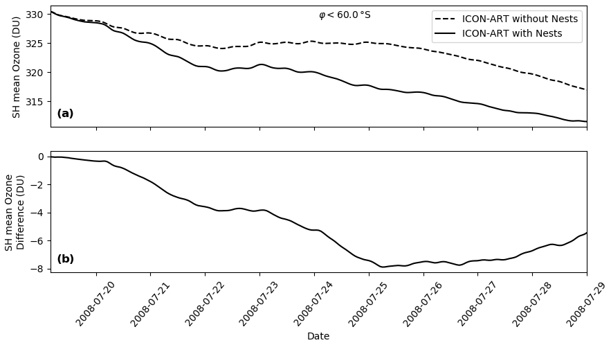
Figure 15 Time series of the mean total ozone column during the third period of the simulation in the global domains for latitudes south of 60^∘ S (a). The dashed line is the simulation without the nests, and the solid line shows the ozone development in the simulation with the nests. The difference between these lines is illustrated in panel (b).

As can be seen, differences in the simulations are below 1 DU during the whole day of 19 July (see also panel b). This first day is a spin-up period for the nests that are initialised with the global domain to form the mountain wave. From 20 July until end of the simulation, however, the mean ozone column in the simulation with the nests is smaller than in the simulation without the nests. While ozone is generally decreasing during this period in both simulations, the absolute value of the difference peaks at around 8 DU on 25 July and decreases afterwards. This order of magnitude has also been simulated by the parameterisation of mountain-wave-induced PSCs of Orr et al. (2020). The higher resolution around Antarctica and the Antarctic Peninsula seems to lead to generally lower ozone columns. This additionally highlights the need for higher resolutions in atmospheric chemistry models.

Figure 15 demonstrates that the higher load of active chlorine species leads to an up to 8 DU larger decrease of ozone in the Southern Hemisphere. The prediction skill after 10 d is fairly low so that an analysis after the shown period is not possible with a free-running simulation. Future investigations could extend this period with specified dynamics in both simulations to be able to examine the impact of mountain-wave-induced PSCs on the ozone hole during September and October.

6 Conclusions and outlook

Seamless modelling of chemistry–climate interactions is challenging. Not many modelling systems can do this in a consistent way. In the past, it was impossible to directly simulate mountain-wave-induced PSCs in global chemistry models due to the coarse resolution in that kind of simulations. In this study, we investigated this problem with the scheme for PSCs in the ICOsahedral Non-hydrostatic modelling framework with its extension for Aerosols and Reactive Trace gases (ICON-ART). The scheme forms ice PSCs based on the microphysics of the meteorological model, liquid (sulfate and STS) particles by the analytic expression of Carslaw et al. (1995) with some improvements with respect to the constant particle number concentration and NAT particles by a kinetic non-equilibrium approach with a flexibly selectable size distribution.

We performed a three-step simulation to investigate the impact of mountain-wave-induced PSCs in ICON-ART on the chemistry: first, a free-running simulation was conducted from 1 March to 30 April 2008. Second, the dynamics were re-initialised every second day by ERA-Interim data to ensure a realistic development of the polar vortex until 18 July 2008. Third, two free-running simulations followed that covered the investigated mountain wave event from 19 to 29 July 2008: a simulation including two-way nesting with nests around Antarctica (Δx≈80 km) and the Antarctic Peninsula (Δx≈40 km) and a simulation without these nests.

The results were compared with measurements by CALIOP and AIRS. The CALIOP PSC categories of ICON-ART were derived from an algorithm that transfers the PSC volume concentrations to the spectral space of CALIOP so that a statistical comparison between both datasets could be established. The total number of grid points with PSCs in ICON-ART was half of that measured by CALIOP although the temperature distribution was similar. This should be further investigated in future simulations. The CALIOP wave ice category could not be simulated with the model, most probably as a result of the constant ice number concentration set to 0.25 cm⁻³. The analyses also showed the need for an interactive calculation of PSCs to treat the different PSC types competing with the available gaseous HNO₃ and H₂O. The comparison with all CALIOP measurements within the Antarctic Peninsula nest demonstrated that the general formation of most of the PSCs in ICON-ART is similar with respect to temperature. We found a resolution-dependent overestimation of the fraction of ice clouds in comparison to CALIOP at high temperatures. This suggested that an even higher resolution is needed to capture PSCs in the lowest temperatures. However, the resolution of 40 km clearly improved the PSC formation compared to 160 km and CALIOP. These findings were also pronounced by evaluations with respect to the NAT and ice formation temperatures.

The comparison to AIRS demonstrated for all Antarctic Peninsula overpasses of 20 and 21 July 2008 that the main features of the mountain wave could be represented at the resolution of 40 km. The measured angle of the mountain wave to the mountain range could be reflected by the model, and the brightness temperature perturbation was in the correct order of magnitude for all overpasses. The investigated mountain wave had a horizontal wavelength of about 300 km that could be captured by the chosen resolution. For mountain waves with smaller wavelengths, an even higher resolution would be needed to resolve the wave adequately.

By introducing the two-way nesting around the Antarctic Peninsula with resolutions down to 40 km, we were able to directly simulate the main features of the mountain wave and transfer its effect back to the global domain. Thus, additional mountain-wave-induced PSCs together with lower temperatures led to enhanced chlorine activation at the global resolution of 160 km. An up to 8 DU larger ozone depletion above the Antarctic continent was simulated.

Thus, this study shows the need to treat mountain-wave-induced PSCs in CCMs. The study also demonstrated that dynamics, tracers, PSCs and chemistry are interactively and consistently integrated in ICON-ART. In addition, ICON-ART showed the potential to bridge the gap between direct simulations of mountain-wave-induced PSCs and their treatment at coarse global resolutions.

Future simulations should exploit the nesting technique further and use it for other known mountain wave hot spots (e.g. Hoffmann et al., 2013, 2017). Waves of non-orographic origin, such as southern hemispheric storm tracks, can also induce mesoscale temperature perturbation that have not been considered in our simulations (e.g. Tritscher et al., 2021). In addition, the impact on ozone depletion should be evaluated with measurements and simulations of longer periods. The Northern Hemisphere should be also a focus in the future where PSC formation and ozone depletion has been shown to be highly sensitive to the existence of mountain waves (e.g. Tabazadeh et al., 2000; Eckermann et al., 2006; Dörnbrack et al., 2012; Khosrawi et al., 2018).

Appendix A: The PSC scheme in ICON-ART

In ICON-ART, the three types of PSCs (ice, NAT and STS) are treated separately. Sensitivity simulations showed that the ICON microphysics for ice clouds, operationally computed up to an altitude of 22.5 km, can be extended to the lower stratosphere up to 30 km (Weimer, 2019). The hydrometeor microphysics in ICON include heterogeneous nucleation of cloud ice, nucleation of cloud ice due to homogeneous freezing of cloud water, and depositional growth and sublimation of cloud ice interacting with the other hydrometeors as well as sedimentation of the ice particles (Doms et al., 2011). Thus, both nucleation of ice PSCs and dehydration of the lower stratosphere can be captured by the ICON microphysics. A similar approach is used in the Whole Atmosphere Community Climate Model (Wegner et al., 2013). Ice particle radius (r_ice in metres) and particle number concentration (N_ice in particles per cubic centimetre) correspond to the assumed size distributions in the microphysics (Doms et al., 2011):

$$\begin{array}{}\text{(A1)}& {\displaystyle }{N}_{\mathrm{ice}}\left(T\right)=min\left(\mathrm{5}\exp \left[\mathrm{0.304}\left(\mathrm{273.15}-T\right)\right],\mathrm{250}\times {\mathrm{10}}^{\mathrm{3}}\right),\text{(A2)}& {\displaystyle }{r}_{\mathrm{ice}}={\displaystyle \frac{\mathrm{1}}{\mathrm{2}}}\sqrt[\mathrm{3}]{\frac{\mathit{\rho }{q}_{\mathrm{ice}}}{\mathrm{130}{N}_{\mathrm{ice}}}},\end{array}$$

where ρ is the air density in kilograms per cubic metre, T is the temperature in kelvin and q_ice is the mass mixing ratio in kilograms per kilogram of water in ice. Equation (A1) means that the ice particle number concentration is assumed to be 0.25 cm⁻³ for temperatures lower than 239 K.

Two parameterisations for the microphysics of NAT particles are integrated in ICON-ART. The thermodynamic NAT parameterisation is diagnostic and therefore computes the number of moles of NAT particles in thermodynamic equilibrium, calculates its sedimentation and evaporates the particles again within the same model time step. The volume mixing ratio of HNO₃ condensed in NAT ($X_{{\mathrm{HNO}}_{\mathrm{3}}\left(\mathrm{NAT}\right)}$ in moles per mole) is calculated on the basis of the difference between vapour pressure of HNO₃ ($p_{{\mathrm{HNO}}_{\mathrm{3}}}$ in pascals) and the saturation vapour pressure over NAT (p_sat,NAT in pascals):

$$\begin{array}{}\text{(A3)}& X_{{\mathrm{HNO}}_{\mathrm{3}}\left(\mathrm{NAT}\right)}={\displaystyle \frac{p_{{\mathrm{HNO}}_{\mathrm{3}}}-p_{\mathrm{sat},\mathrm{NAT}}}{p}}.\end{array}$$

The saturation vapour pressure over NAT is calculated according to Hanson and Mauersberger (1988), and p is the air pressure (in pascals). Particle number concentration (N_NAT) and radius (r_NAT) in the thermodynamic NAT parameterisation are calculated using a threshold in the number concentration of $N_{\mathrm{NAT},\max }=\mathrm{2.3}\times {\mathrm{10}}^{-\mathrm{4}}{\mathrm{cm}}^{-\mathrm{3}}$, which is based on van den Broek et al. (2004). Below this threshold, the radius of the NAT particles is set to 0.1 µm. Above this threshold, the particle number concentration is set to N_NAT,max, and the radius of the particles is increased accordingly. This method has already been used in a similar way for solid particles by Kirner et al. (2011).

The kinetic NAT parameterisation is a non-equilibrium approach based on prognostic equations for the particle mass (see e.g. Seinfeld and Pandis, 2006, p. 539). Carslaw et al. (2002) applied this approach to NAT particles in a Lagrangian model, and van den Broek et al. (2004) extended it to Eulerian models.

In the Lagrangian description by Carslaw et al. (2002), the change in NAT particle radius (r_NAT,b) is calculated prognostically by a diffusive growth:

$$\begin{array}{}\text{(A4)}& {\displaystyle \frac{\mathrm{d}{r}_{\mathrm{NAT},b}}{\mathrm{d}t}}={\displaystyle \frac{G_b}{r_{\mathrm{NAT},b}}},\end{array}$$

where G_b (in square metres per second) is a growth factor which depends on the diffusion coefficient of HNO₃ in air ($D_{{\mathrm{HNO}}_{\mathrm{3}}}$ in square metres per second), the air temperature (T in kelvin) and the saturation difference of the HNO₃ vapour pressure (in pascals):

$$\begin{array}{}\text{(A5)}& G_b={\displaystyle \frac{D_{{\mathrm{HNO}}_{\mathrm{3}},b}^{*}{M}_{\mathrm{NAT}}}{{\mathit{\rho }}_{\mathrm{NAT}}{R}^{*}T}}\left(p_{{\mathrm{HNO}}_{\mathrm{3}}}-p_{\mathrm{sat},\mathrm{NAT}}\right),\end{array}$$

with

$$\begin{array}{}\text{(A6)}& D_{{\mathrm{HNO}}_{\mathrm{3}},b}^{*}={\displaystyle \frac{D_{{\mathrm{HNO}}_{\mathrm{3}}}}{\mathrm{1}+\mathrm{4}{D}_{{\mathrm{HNO}}_{\mathrm{3}}}/\left({\stackrel{\mathrm{‾}}{v}}_{{\mathrm{HNO}}_{\mathrm{3}}}{r}_{\mathrm{NAT},b}\right)}}.\end{array}$$

In these equations, ${\stackrel{\mathrm{‾}}{v}}_{{\mathrm{HNO}}_{\mathrm{3}}}$ is the mean thermal velocity of air molecules (in metres per second), R^* stands for the universal constant of an ideal gas in joules per mole per kelvin (J mol⁻¹ K⁻¹), ρ_NAT is the crystal density of NAT ($\mathrm{1.626}\times {\mathrm{10}}^{\mathrm{6}}\mathrm{g}{\mathrm{m}}^{-\mathrm{3}}$; Drdla et al., 1993; van den Broek et al., 2004) and M_NAT is the NAT molar mass of 117 g mol⁻¹. In one of the Eulerian formulations by van den Broek et al. (2004), this radius change is applied to particles in size bins, but directly converted into a change in the particle number concentration (“FixedRad” approach). This approach is used in this study with a size distribution based on van den Broek et al. (2004) as shown in Fig. 3. That is why we added a b subscript to all variables in Eqs. (A4), (A5) and (A6) that depend on the size bin b.

The size distribution of NAT particles can be flexibly specified by the user to investigate its impact on denitrification without any change in the Fortran code but rather changing the respective XML control file (cf. Schröter et al., 2018). Each size bin is defined by radius limits and a maximum particle number concentration, which are kept constant during the simulation. If the calculated particle number concentration in a bin exceeds the maximum, the excess mass is transferred to the next larger size bin. The sum of the maximum particle number concentrations of the bins has to equal the value by van den Broek et al. (2004), which is $\mathrm{2.3}\times {\mathrm{10}}^{-\mathrm{4}}{\mathrm{cm}}^{-\mathrm{3}}$ and based on measurements of large NAT particles. Sensitivity studies by van den Broek et al. (2004) showed that this value in combination with the size distribution used leads to denitrification comparable to measurements. The size bins are transported as passive tracers in ICON-ART.

Since the calculation of p_sat,NAT by Hanson and Mauersberger (1988) has specific temperature limits, NAT particles are evaporated automatically at temperatures higher than 220 K. For temperatures below 180 K, we calculate $p_{{\mathrm{HNO}}_{\mathrm{3}}}$ with a constant temperature of 180 K. These two NAT parameterisations are also implemented in EMAC (Jöckel et al., 2010; Kirner et al., 2011).

Sedimentation of NAT particles, formed by either thermodynamic or kinetic NAT parameterisation, is calculated by a simple upwind method, using the Stokes velocity of assumed spherical particles (Stokes, 1851).

The microphysics of liquid (sulfate and STS) particles in the module are calculated by the scheme first published by Carslaw et al. (1995), with one exception: in the original code by Carslaw et al. (1995) the particle number concentration is set to the constant value of 10 cm⁻³. We improved this fixed value by applying the mean of all balloon-borne STS measurements by Hervig and Deshler (1998) in order to derive the particle surface area concentration S_STS and the radius r_STS of STS particles from the internally calculated particle volume concentration V_STS:

$$\begin{array}{}\text{(A7)}& {\displaystyle }{S}_{\mathrm{STS}}& {\displaystyle }=\mathrm{6.068}(V_{\mathrm{STS}}{)}^{\mathrm{0.671}},\text{(A8)}& {\displaystyle }{r}_{\mathrm{STS}}& {\displaystyle }={\displaystyle \frac{\mathrm{3}{V}_{\mathrm{STS}}}{S_{\mathrm{STS}}}}.\end{array}$$

In these equations, V_STS has to be given in cubic micrometres per cubic centimetre (µm³ cm⁻³) to get S_STS and r_STS in square micrometres per cubic centimetre (µm² cm⁻³) and micrometres, respectively. Sedimentation is neglected for liquid particles since they are too small to result in relevant redistribution of the major constituents H₂O, HNO₃ and H₂SO₄ (Tabazadeh et al., 2000; Considine et al., 2000).

Since the PSCs in the current version of the model do not interact with each other like in a fully coupled PSC scheme (e.g. Zhu et al., 2015), there are essentially two approaches to calculating PSCs: either they are computed with the total (gaseous + liquid + solid) concentrations of HNO₃ and H₂O as input for all PSC types (e.g. Kirner et al., 2011) or the PSCs are calculated subsequently with the gaseous fraction that remains after formation of the previously calculated PSC types (operator splitting). Both approaches have their advantages and disadvantages. We use the second approach because the maximum of HNO₃ and H₂O taken up by PSCs cannot exceed the gaseous concentrations in this case. First, ice PSCs are calculated, then NAT PSCs and finally liquid particles.

Particle radius, particle number concentration and particle surface area concentration are used to calculate the heterogeneous reaction rate constants on the surface of PSCs. For NAT and ice, which can grow to relatively large sizes in the order of tens of micrometres, the following equation is used to calculate the heterogeneous reaction rate constant, assuming spherical particles (Drdla et al., 1993):

$$\begin{array}{}\text{(A9)}& k_{\mathrm{het},h,c}={\displaystyle \frac{{\mathit{\gamma }}_{h,c}\mathit{\pi }{r}_c^{\mathrm{2}}{\stackrel{\mathrm{‾}}{v}}_{i\left(h\right)}{N}_c}{N_{j\left(h\right)}\left(\mathrm{1}+\frac{\mathrm{3}{\mathit{\gamma }}_{h,c}}{\mathrm{4}Kn}\right)}},c\in \left\{\mathrm{NAT},\mathrm{ice}\right\},\end{array}$$

where γ_h,c is the uptake coefficient (i.e. reaction probability) of heterogeneous reaction h and PSC type c, ${\stackrel{\mathrm{‾}}{v}}_{i\left(h\right)}$ is the mean thermal velocity of the gaseous reactant i(h) (in metres per second), N_c is the PSC number concentration and N_j(h) is the number concentration of the reactant j(h) adsorbed on the particle (both per cubic metre). The Knudsen number Kn is calculated by ${\mathit{\lambda }}_{\mathrm{mfp}}/r_c$ with the mean free path λ_mfp of air molecules (in metres), calculated according to Kennard (1938). In the case of the kinetic NAT parameterisation, Eq. (A9) is evaluated for each size bin separately and summed up subsequently.

Liquid particles are considerably smaller than ice and NAT particles (e.g. Considine et al., 2000), and hence Kn≫1, so that the slip flow correction term in Eq. (A9) can be neglected, which yields

$$\begin{array}{}\text{(A10)}& k_{\mathrm{het},h,\mathrm{liq}}={\displaystyle \frac{{\mathit{\gamma }}_{h,\mathrm{liq}}{\stackrel{\mathrm{‾}}{v}}_{i\left(h\right)}{S}_{\mathrm{liq}}}{\mathrm{4}{N}_{j\left(h\right)}}}.\end{array}$$

The total reaction rate constant is the sum of the reaction rate constants on all three types of PSCs. The uptake coefficients in ICON-ART are used either from Carslaw et al. (1995) or Sander et al. (2011b). A summary of the γ values can be found in Table S3 of the paper's Supplement. They also compare well to other models (e.g. Solomon et al., 2015).