Quantifying variability, source, and transport of CO in the urban areas over the Himalayas and Tibetan Plateau

Atmospheric pollutants over the Himalayas and Tibetan Plateau (HTP) have potential implications for accelerating the melting of glaciers, damaging air quality, water sources and grasslands, and threatening climate on regional and global scales. Improved knowledge of the variabilities, sources, drivers and transport pathways of atmospheric pollutants over the HTP is significant for regulatory and control purposes. In this study, we quantify the variability, source, and transport of CO in the urban areas over the HTP by using in situ measurement, GEOS-Chem model tagged CO simulation, and the analysis of meteorological fields. Diurnal, seasonal, and interannual variabilities of CO over the HTP are investigated with ∼ 6 years (January 2015 to July 2020) of surface CO measurements in eight cities over the HTP. Annual mean of surface CO volume mixing ratio (VMR) over the HTP varied over 318.3 ± 71.6 to 901.6 ± 472.2 ppbv, and a large seasonal cycle was observed with high levels of CO in the late autumn to spring and low levels of CO in summer to early autumn. The diurnal cycle is characterized by a bimodal pattern with two maximums in later morning and midnight, respectively. Surface CO VMR from 2015 to 2020 in most cities over the HTP showed negative trends. The IASI satellite observations are for the first time used to assess the performance of the GEOS-Chem model for the specifics of the HTP. The GEOS-Chem simulations tend to underestimate the IASI observations but can capture the measured seasonal cycle of CO total column over the HTP. Distinct dependencies of CO on a short lifetime species of NO₂ in almost all cities over the HTP were observed, implying local emissions to be predominant. By turning off the emission inventories within the HTP in GEOS-Chem tagged CO simulation, the relative contribution of long-range transport was evaluated. The results showed that transport ratios of primary anthropogenic source, primary biomass burning (BB) source, and secondary oxidation source to the surface CO VMR over the HTP varied over 35 % to 61 %, 5 % to 21 %, and 30 % to 56 %, respectively. The anthropogenic contribution is dominated by the South Asia and East Asia (SEAS) region throughout the year (58 % to 91 %). The BB contribution is dominated by the SEAS region in spring (25 % to 80 %) and the Africa (AF) region in July–February (30 %–70 %). This study concluded that the main source of CO in urban areas over the HTP is due to local and SEAS anthropogenic and BB emissions and oxidation sources, which differ from the black carbon that is mainly attributed to the BB source from South-East Asia. The decreasing trends in surface CO VMR since 2015 in most cities over the HTP are attributed to the reduction in local and transported CO emissions in recent years.

1 Introduction

The Himalayas and Tibetan Plateau (HTP), also named the “Third Pole” (TP), is an important region for climate change studies for several reasons. Due to its unique feature for interactions among the atmosphere, biosphere, hydrosphere, and cryosphere, the HTP is referred to as an important indicator of regional and global climate change (Pu et al., 2007; Yao et al., 2012; Zhang et al., 2015). The HTP stores a large amount of ice masses on the planet and provides the headwater of many Asian rivers which contribute water resources to over 1.4 billion people, and it thus is referred to as the “Water Tower of Asia” (Xu et al., 2008; Immerzeel et al., 2010; Gao et al., 2019; Kang et al., 2019). The glaciers and snowmelt over the HTP can potentially modify the regional hydrology, contribute to global sea-level rise, and trigger natural hazards which may threaten the health and wealth of many populations (Singh and Bengtsson, 2004; Barnett et al., 2005; Immerzeel et al., 2010; Kaser et al., 2010; Bolch et al., 2012; Yao et al., 2012; Gao et al., 2019). The HTP has an average altitude of about 4000 m above sea level (a.s.l.), which highly elevates topography of the earth system and imposes profound effects on global atmospheric circulation and climate change (Ye and Wu, 1998; Wu et al., 2012; Zhang et al., 2015; Kang et al., 2019). The HTP is also of great interest for model validation, since the extreme climate conditions and the variability between clean and polluted conditions in the region are a challenge for current chemical transport models (Ye et al., 2012; Kopacz et al., 2011; Zhang et al., 2015).

Since the population level is very low, the HTP has long been regarded as an atmospheric background with negligible local anthropogenic emissions (Yao et al., 2012; Kang et al., 2019). However, the HTP is surrounded by East Asia and South Asia, which include many intensive anthropogenic and natural emission source regions (Zhang et al., 2015; Kang et al., 2019). The transport of polluted air masses from the highly populated area in northern India with its industry and agriculture can have a strong impact on the composition of the atmosphere (Cong et al., 2009; Kang et al., 2019). Furthermore, the Asian monsoon has a strong influence on the dynamics and transport pathways in the HTP (Zhang et al., 2015; Kang et al., 2019). Reanalysis results based on glacial ice cores and lake sediments have revealed distinguishable anthropogenic disturbances from Asian emissions since the 1950s (Wang et al., 2008; Cong et al., 2013; Zhang et al., 2015; Kang et al., 2016, 2019). Convective transport around the HTP areas has also been verified by satellite observations, chemical transport model simulations, flask sampling analyses, and in situ measurements of some key atmospheric constituents. These atmospheric constituents include carbon monoxide (CO) (Park et al., 2007, 2008), methane (CH₄) (Xiong et al., 2009), hydrogen cyanide (HCN) (Randel et al., 2010), polyacrylonitrile (PAN) (Zhang et al., 2009; Ungermann et al., 2016; Xu et al., 2018), ozone (O₃) (Yin et al., 2017; Xu et al., 2018), and aerosol (Cong et al., 2007, 2009, 2013; He et al., 2014; Zhang et al., 2015; Zhu et al., 2019; Li et al., 2021; Gul et al., 2021; Thind et al., 2021). Furthermore, urbanization, industrialization, land use, and infrastructure construction over the HTP have expanded rapidly in recent years, which could also emit air pollutants into the atmosphere (Ran et al., 2014; X. Yin et al., 2019).

The ecosystem over the HTP is sensitive and fragile under the extreme alpine conditions. These exogenous and local atmospheric pollutants have potential implications for accelerating the melting of glaciers, damaging air quality, water sources, and grasslands, and threatening climate on regional and global scales (Pu et al., 2007; Xu et al., 2009; Yao et al., 2012; Kang et al., 2016; H. Yin et al., 2019, 2020; X. Yin et al., 2019). Efforts have been made to understand the variabilities of atmospheric pollutants over the HTP. However, due to the logistic difficulties and poor accessibility of the vast HTP, most studies are based on episodic measurements in specific regions or at widely dispersed sites (Kang et al., 2019). An inter-comparison of these data and deductions may show large inconsistencies and uncertainties because the reported individual studies have often relied on different instruments and techniques (Kang et al., 2019). In addition, most previous studies have often concentrated on burdens, sources, and transport of carbonaceous aerosols, including organic carbon (OC) and black carbon (BC), over the HTP, but the studies on gaseous pollutants are limited (Cong et al., 2007, 2009, 2013; He et al., 2014; Zhang et al., 2015; Zhu et al., 2019; Li et al., 2021; Gul et al., 2021; Thind et al., 2021). As a result, the variabilities, sources, drivers, and transport pathways of atmospheric pollutants over the HTP are still not fully understood.

CO is one of the most critical atmospheric pollutants and not only threatens human health, but also plays a vital role in atmospheric chemistry (Zhang et al., 2019; Zheng et al., 2019). CO has a long atmospheric residence time of a few months and is therefore established as a key tracer for air pollution and transport in the atmosphere (Holloway et al., 2000; Zheng et al., 2019). Natural sources such as biomass burning (BB) and anthropogenic sources such as vehicle exhausts, industrial activities, and coal combustions can emit CO directly into the atmosphere (Stremme et al., 2013; Fisher et al., 2017). These CO emissions are mainly attributed to incomplete combustion (Holloway et al., 2000; Stremme et al., 2013). Furthermore, the atmospheric oxidation of methane (CH₄) and numerous non-methane VOCs (NMVOCs) provides additional important sources of atmospheric CO (Fisher et al., 2017). The major CO sink in the troposphere is oxidation via reaction with hydroxyl radicals (OH). Since CO is heavily involved in the relationship between atmospheric chemistry and climate forcing, it is crucial to investigate its atmospheric burden, variability, and potential driver over the HTP. CO over the HTP may originate from various source regions and sectors; improved knowledge of their relative contributions to CO variability over the HTP is also significant for regulatory and control purposes. Furthermore, an investigation of CO pollution can complement current atmospheric investigation over the HTP since the chemical characteristic, climate forcing, and deletion of CO are different from the well-established carbonaceous aerosols.

In this study, we quantify the variability, source, and transport of CO in the urban areas over the HTP by using in situ measurement, GEOS-Chem model tagged CO simulation, and atmospheric circulation pattern techniques. Diurnal, seasonal, and interannual variabilities of CO over the HTP are investigated with multiyear time series of surface CO measurements in eight cities over the HTP. The performance of the GEOS-Chem full-chemistry model for the specifics of the HTP is first assessed with the concurrent satellite observations. The GEOS-Chem model is then run in a tagged CO mode to quantify the relative contribution of long-range transport to the observed CO variability over the HTP. The three-dimensional (3D) transport pathways of CO originating in various source regions and sectors to the HTP are finally determined by the GEOS-Chem simulation, back-trajectory analysis, and atmospheric circulation pattern. Only a few studies have investigated the burden and variability of CO over the HTP (Ran et al., 2014; H. Yin et al., 2019). These studies uniformly focused on the most developed regions in Lhasa and did not analyse interannual trends and transport of CO. This study not only expands the coverage of CO quantification over the HTP, but also provides insights into the interannual trends, sources, and transport of CO in all urban areas over the HTP.

The next section gives a site description, the surface in situ CO data and auxiliary data, the methodology used to estimate the interannual trend of surface CO, and the GEOS-Chem simulation used for source attribution. Section 3 reports the results for surface CO variability over the HTP on different timescales. Section 4 presents the results for GEOS-Chem model evaluation. Section 5 analyses the results for source attribution using GEOS-Chem tagged CO simulation and the analysis of meteorological fields. We conclude the study in Sect. 6.

2 Methods and data

2.1 Site description

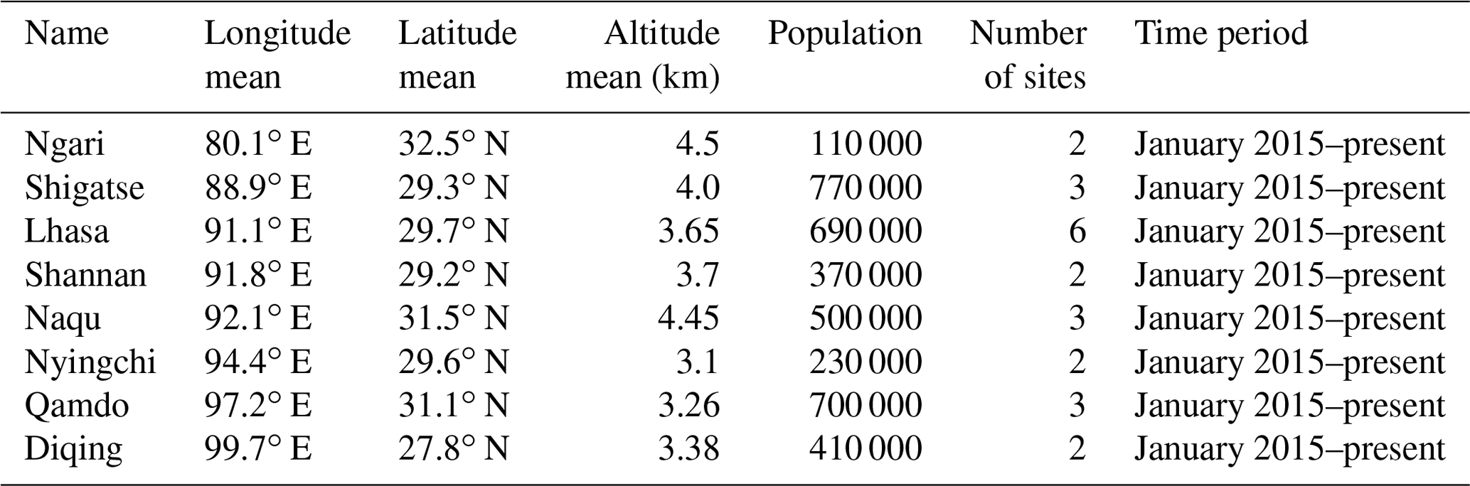
Surface in situ CO measurements in eight cities over the HTP are used in this study. The locations of these cities are shown in Fig. 1 and summarized in Table 1. Ngari is located in the west, Diqing and Qamdo are located in the east, and the remaining cities are all in the central east of the HTP. Ngari, Shigatse, Lhasa, Shannan, and Nyinchi are adjacent to the Himalayas region, and Naqu, Qamdo, and Diqing are relatively distant from the Himalayas region. Generally, these cities represent the most developed and populated areas over the HTP. The altitude of these cities ranges from 3.1 to 4.5 km a.s.l., and the population ranges from 110 000 to 770 000​​​​​​​. The surface pressure of these cities is about 600 hPa or less throughout the year (Table 1). Typically, all these cities are formed in flat valleys, with the surrounding mountains rising to more than 5.0 km a.s.l., and have continuous expansion and development over time. These cities are characterized by a typical climate regime in high mountain regions and are dry and cold in most of the year. Due to the high altitude and thin air, incident solar radiations over these cities are stronger than those over other cities at the same latitude around the globe (Ran et al., 2014).

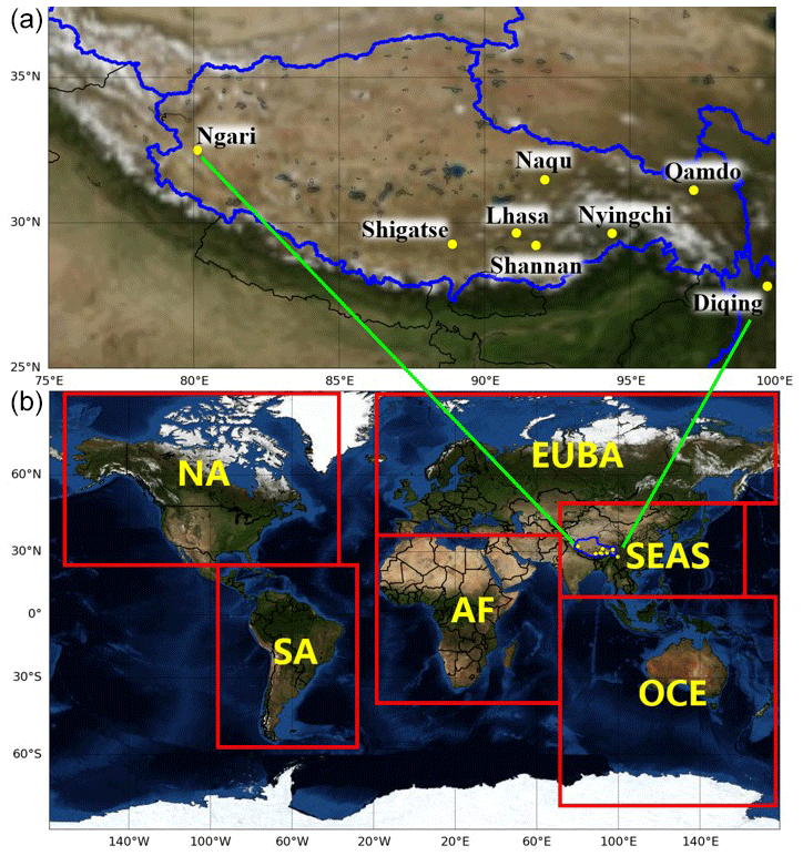
Figure 1 Enlarged view for geolocations of all cities (yellow dots) over the Himalayas and Tibetan Plateau (HTP) (a). Geographical regions implemented in the standard GEOS-Chem tagged CO simulation (b). Latitude and longitude definitions are listed in Table 2. The base map is created by the Basemap package of Python.

Table 1 Geolocations of measurement sites in eight cities over the HTP region. All sites are organized as a function of increasing longitude. Population statistics are prescribed from the 2018 demographic data provided by National Bureau of Statistics of China.

General atmospheric circulations over these cities are typically influenced by three synoptic systems: the warm and wet air masses during the monsoon season in summer, the South Asian anticyclone that controls the upper troposphere and above, and the subtropical mid-latitude westerlies in winter (Yao et al., 2012; Ran et al., 2014; Yin et al., 2017). Inhibited by surrounding mountains, local mountain peak–valley wind systems facilitate the accumulation of atmospheric pollutants near the ground under low wind speed conditions (Kang et al., 2019).

2.2 Surface CO data and auxiliary data

Routine in situ measurement of surface air qualities over the HTP started in 2015, which are organized by the China National Environmental Monitoring Center (CNEMC) network funded by the Chinese Ministry of Ecology and Environment (http://www.cnemc.cn/en/, last access: 22 March 2020). The CNEMC network has monitored six surface air pollutants (including CO, O₃, NO₂, SO₂, PM₁₀, and PM_2.5) at 23 sites in eight cities in Ngari, Lhasa, Naqu, Diqing, Shigatse, Shannan, Nyingchi, and Qamdo over the HTP (Table 1). Each city has at least two measurement sites. Surface CO volume mixing ratio (VMR) measurements at all sites are based on similar gas correlation filter infrared analysers (http://www.cnemc.cn/en/). The hourly mean datasets have covered the period from January 2015 to present for all measurement sites in the eight cities (Table 1). We first applied filter criteria following that of Lu et al. (2019) to remove unreliable measurements. The resulting measurements at all measurement sites in each city are then averaged to obtain a city-representative dataset.

The 3D back trajectories calculated using the HYbrid Single-Particle Lagrangian Integrated Trajectory (HYSPLIT) model (http://ready.arl.noaa.gov/HYSPLIT.php, last access: 23 May 2020) are used to determine the transport trajectories (Wang, 2014). The input gridded meteorological fields were from the Global Data Assimilation System (GDAS-1) operated by the US National Oceanic and Atmospheric Administration (NOAA) with a horizontal resolution of 1^∘ latitude × 1^∘ longitude and 23 vertical grids from 1000 to 20 hPa (https://ready.arl.noaa.gov/gdas1.php, last access: 23 May 2020). We verified that the wind fields provided by GDAS-1 are in good agreement with those provided by the Goddard Earth Observing System-Forward Processing (GEOS-FP) meteorological fields used in GEOS-Chem (Fig. S1 in the Supplement). In this study, calculation and analysis for all back trajectories are based on the TrajStat module (Wang, 2014; http://meteothink.org/index.html, last access: 1 July 2020).

The monthly IASI/Metop-A CO dataset version 6.5.0 is used to evaluate the performance of the GEOS-Chem model for the specifics of the HTP. The IASI CO product is processed by the EUMETSAT Application Ground Segment using the Fast Optimal Retrievals on Layers for IASI (FORLI) software (Hurtmans et al., 2012). The IASI CO retrievals are performed in the 2143–2181.25 cm⁻¹ spectral range using the optimal estimation method and tabulated absorption cross sections at various pressures and temperatures to speed up the radiative transfer calculation. A single a priori profile is used in the retrieval scheme (Clerbaux et al., 2009). The temperature, pressure, humidity profiles, and cloud fractions used in FORLI are those from the EUMETSAT Level 2 processor. Only pixels associated with cloud fractions below 25 % are processed. The IASI CO product is a vertical profile given as partial columns in moles per square metre in 18 layers between the surface and 18 km, with an extra layer from 18 km to the top of the atmosphere. The pressure levels associated with retrieval layers are provided with the CO product. This IASI CO dataset also includes other relevant information such as a general quality flag, the a priori profile, the total error profile, the air partial column profile, and the averaging kernel (AK) matrix, on the same vertical grid, and the total column and the associated total error. To balance the accuracy and the number of valid data over the HTP, the IASI data within the ±1^∘ latitude–longitude rectangular area around each city and with a total error of less than 15 % are selected.

2.3 Regression model for CO trend

We have used a bootstrap resampling model to determine the seasonality and interannual variability of surface CO VMR over the HTP. The resampling methodology follows that of Gardiner et al. (2008), where a third Fourier series plus a linear function was used to fit multiyear time series of the surface CO VMR biweekly mean. All measurements are averaged by 2 weeks to lower the residual and improve the fitting correlation. The regression model is expressed by Eqs. (1) and (2):

$$\begin{array}{}\text{(1)}& {\displaystyle }{Y}^{\mathrm{meas}}\left(t\right)=Y^{\mathrm{mod}}\left(t\right)+\mathit{\epsilon }\left(t\right),\text{(2)}& {\displaystyle }\begin{array}{rl}{Y}^{\mathrm{mod}}\left(t\right)& =A_{\mathrm{0}}+A_{\mathrm{1}}t+A_{\mathrm{2}}\cos \left({\displaystyle \frac{\mathrm{2}\mathit{\pi }t}{\mathrm{365}}}\right)+A_{\mathrm{3}}\sin \left({\displaystyle \frac{\mathrm{2}\mathit{\pi }t}{\mathrm{365}}}\right)\\ & +A_{\mathrm{4}}\cos \left({\displaystyle \frac{\mathrm{4}\mathit{\pi }t}{\mathrm{365}}}\right)+A_{\mathrm{5}}\sin \left({\displaystyle \frac{\mathrm{4}\mathit{\pi }t}{\mathrm{365}}}\right),\end{array}\text{(3)}& {\displaystyle }\mathrm{d}\mathit{\%}={\displaystyle \frac{Y^{\mathrm{meas}}\left(t\right)-Y^{\mathrm{mod}}\left(t\right)}{Y^{\mathrm{mod}}\left(t\right)}}\times \mathrm{100},\end{array}$$

where Y^meas(t) and Y^mod(t) represent the measured and fitted surface CO VMR time series, respectively. A₀ is the intercept, A₁ is the annual growth rate, and $A_{\mathrm{1}}/A_{\mathrm{0}}$ is the interannual trend discussed below. In this study, we incorporated the errors arising from the autocorrelation in the residuals into the uncertainties in the trends following the procedure of Santer et al. (2008). The A₂–A₅ parameters describe the seasonal cycle, t is the measurement time elapsed since January 2015, and ε(t) represents the residual between the measurements and the fitted results. Fractional differences of measured CO VMR time series relative to their seasonal mean values represented by Y^mod(t) were referred to as seasonal enhancements and were calculated as Eq. (3).

2.4 GEOS-Chem simulation

Two types of GEOS-Chem model simulations were involved in this study. GEOS-Chem model version 12.2.1 (https://doi.org/10.5281/zenodo.2580198, The International GEOS-Chem Community, 2019​​​​​​​) was first run in a standard full-chemistry mode to be evaluated by the IASI CO product. The GEOS-Chem model was then run in a standard tagged CO mode to quantify the relative contribution of long-range transport to the observed CO variability over the HTP (Bey et al., 2001) (http://geos-chem.org, last access: 14 May 2020). The GEOS-Chem full-chemistry simulations were also used to provide OH fields and secondary CO production rates from CH₄ and NMVOC oxidation for subsequent GEOS-Chem tagged CO simulation. Both types of simulations were driven by GEOS-FP meteorological fields with a downgraded horizontal resolution of 2^∘ latitude × 2.5^∘ longitude and 72 vertical grids from the surface to 0.01 hPa. Surface meteorological variables and planetary boundary layer height (PBLH) were implemented in a 1 h interval and other meteorological variables were in a 3 h interval. The time steps used in the model are 10 min for transport and 20 min for chemistry and emissions, as recommend for the GEOS-Chem full-chemistry simulation at 2 × 2.5 (Philip et al., 2016). The non-local schemes for the boundary-layer mixing process are described in Lin and McElroy (2010). The GEOS-Chem simulation outputs 47 (tagged CO mode) or 72 (full-chemistry mode) vertical layers of CO VMR concentration ranging from the surface to 0.01 hPa with a horizontal resolution of 2^∘ × 2.5^∘ and a temporal resolution of 1 h (Sun et al., 2021). We spun up the model for 1 year (January 2014 to January 2015) to remove the influence of the initial conditions. We only considered CO simulations for the grid boxes containing the eight cities over the HTP.

Global fossil fuel and biofuel emissions were from the Community Emissions Data System (CEDS) inventory (Hoesly et al., 2018) and are replaced by regional emissions over the US by the National Emission Inventory (NEI), Canada by Canadian Criteria Air Contaminant, Mexico by​​​​​​​ Kuhns et al. (2005), Europe by the European Monitoring and Evaluation Program (EMEP), East Asia and South Asia by the MIX inventory (Li et al., 2017; Zheng et al., 2018; Lu et al., 2019), and Africa by the DICE-Africa inventory (Marais and Wiedinmyer, 2016). Global BB emissions are derived from the Global Fire Assimilation System (GFAS) v1.2 (Kaiser et al., 2012; Di Giuseppe et al., 2018). The soil NO_x emissions were from Hudman et al. (2010, 2012). Biogenic emissions were from the Model of Emissions of Gases and Aerosols from Nature (MEGAN version 2.1) inventory (Guenther et al., 2012). Wet deposition followed that of Liu et al. (2001) and dry deposition was calculated by the resistance-in-series algorithm (Wesely, 1989; Zhang et al., 2001). The photolysis rates were obtained from the FAST-JX v7.0 photolysis scheme (Bian and Prather, 2002). A universal tropospheric–stratospheric chemistry (UCX) mechanism was implemented (Eastham et al., 2014).

Table 2 Descriptions of all tracers implemented in the standard GEOS-Chem tagged CO simulation and the geographical definitions of all source regions.

In GEOS-Chem tagged CO simulation, the improved secondary CO production scheme of Fisher et al. (2017) was implemented, which adopts secondary CO production rates from CH₄ and NMVOC oxidation. The monthly mean OH fields and secondary CO production rates from CH₄ and NMVOC oxidation are archived from the full-chemistry simulation of this study. The GEOS-Chem tagged CO simulation includes the tracers of primary anthropogenic (fossil fuel + biofuel) and BB sources and secondary oxidations from CH₄ and NMVOCs. Descriptions of all these tracers are summarized in Table 2, and the geographical definitions of all the source regions are shown in Fig. 1.

3 Surface CO variability over the HTP

3.1 Diurnal cycle

Diurnal cycles of surface CO VMR over the HTP within the period of 2015–2020 are shown in Fig. 2. The surface CO magnitudes and the hour-to-hour variations in Naqu, Qamdo, and Diqing are higher than those in other cities in all seasons. Furthermore, the daily peak-to-trough contrasts in Naqu, Qamdo, and Diqing are also larger than those in other cities. The highest surface CO hourly means are typically observed in Naqu in all seasons except in the second half-day (after 12:00 local time, LT) in autumn and winter (September–October–November/December–January–February, SON/DJF), when the highest surface CO values are observed in Qamdo.

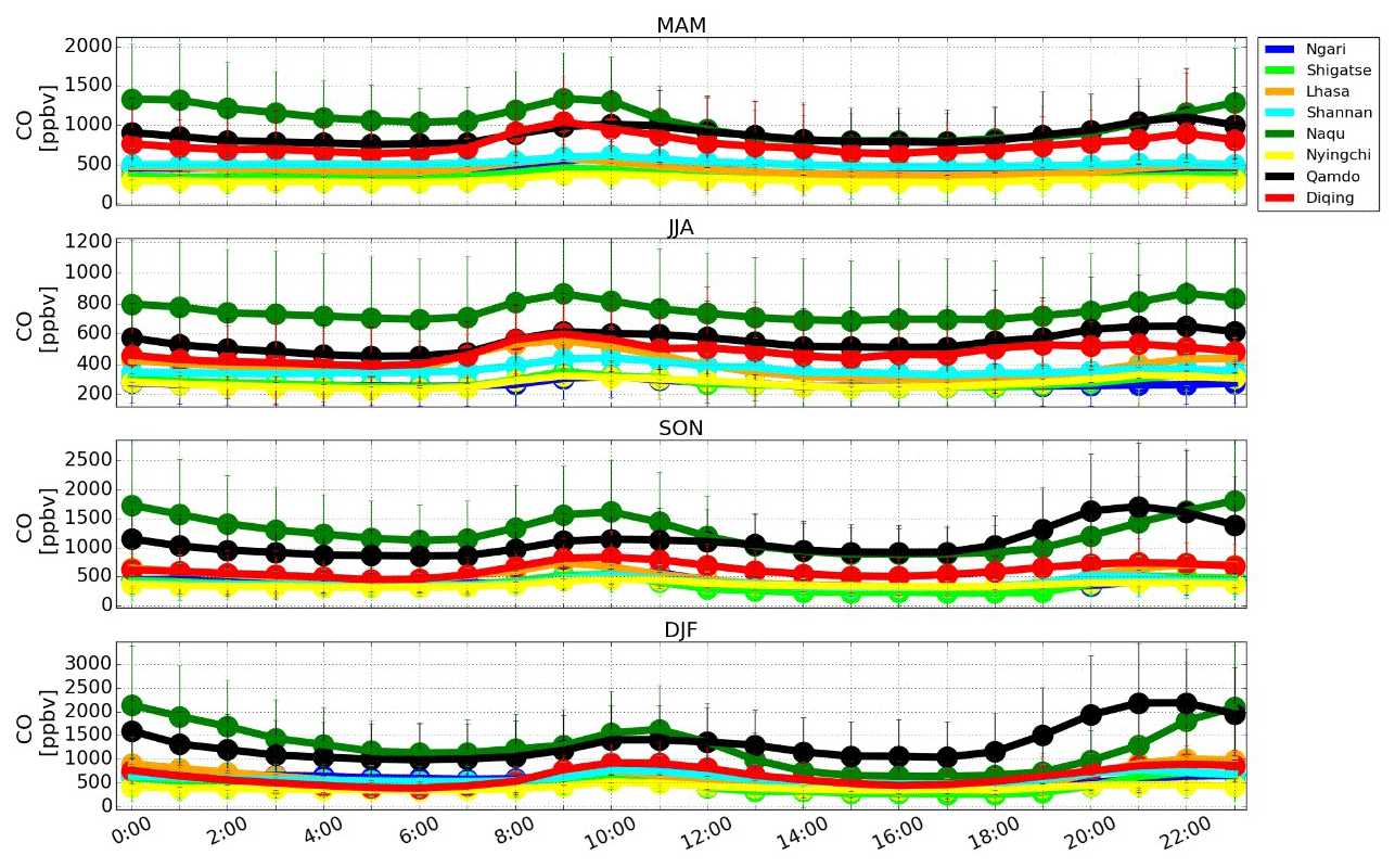
Figure 2 Diurnal cycles (local time, LT) of surface CO VMR in four seasons over the HTP. The vertical error bar is 1σ standard variation within that hour. Results are based on CO time series from 2015 to 2020 provided by the CNEMC network.

Table 3 Statistical summary of surface CO VMR in eight cities over the HTP region. All cities are organized as a function of increasing longitude.

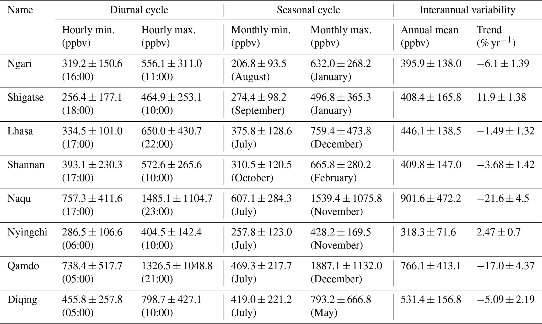
Diurnal cycles of surface CO VMR in all cities generally show a bimodal pattern in all seasons. For all cities, two diurnal maximums are generally observed during 09:00 to 11:00 LT in the daytime and 21:00 to 23:00 LT in the nighttime in all seasons. The timings of the daytime diurnal maximum in spring and summer (March–April–May/June–July–August, MAM/JJA) in all cities are 1 to 2 h earlier than those in SON/DJF (Table 3). However, the timings of the nighttime diurnal maximum in MAM/JJA in all cities are 1 to 2 h later than those in SON/DJF. On average, the diurnal hour-to-hour variation of surface CO VMR over the HTP spanned a large range of −47.7 % to 50.6 % depending on region, season, and measurement time. The diurnal patterns of CO in all cities over the HTP were similar to those in other cities in China (X. Yin et al., 2019; Zhao et al., 2016). Surface CO VMR hourly means in Naqu, Qamdo, and Diqing varied over 455.8 ± 257.8 to 1485.1 ± 1104.7 ppbv, while other cities varied over 256.4 ± 177.1 to 650.0 ± 430.7 ppbv (Table 3). The Class-1 limit for the hourly mean CO concentration in China is 10 mg m⁻³ (8732.1 ppbv) and all hourly mean CO VMRs from 2015 to 2020 over the HTP were below this limit (http://www.cnemc.cn/en/).

3.2 Seasonal cycle

Seasonal cycles of surface CO VMR over the HTP within the period of 2015 to 2020 are shown in Fig. 3. As generally observed in most cities over the HTP, surface CO VMR showed clear seasonal features: (1) high levels of surface CO VMR occur in the late autumn to spring and low levels of surface CO occur in summer to early autumn; (2) the variations in the late autumn to spring are larger than those in summer to early autumn; (3) seasonal cycles of surface CO VMR in most cities show a bimodal pattern; i.e. a large seasonal peak occurs around November–December and a small seasonal peak occurs around April–May.

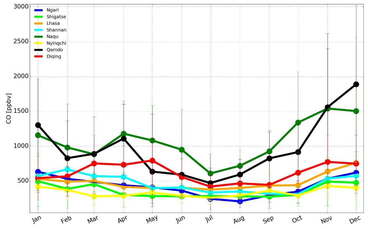
Figure 3 Monthly mean of surface CO VMR over the HTP. Vertical error bar represents 1σ standard variation within that month. Results are based on CO VMR time series from 2015 to 2020 provided by the CNEMC network.

Surface CO VMR monthly mean and month-to-month variations in Naqu, Qamdo, and Diqing are higher than those in other cities in all seasons. Furthermore, the peak-to-trough contrasts in Naqu, Qamdo, and Diqing were also larger than those in other cities. Surface CO VMR monthly mean over the HTP varied over a large range of 206.8 ± 93.5 to 1887.1 ± 1132.0 ppbv depending on season and region (Table 3), where Naqu, Qamdo, and Diqing varied over 419.0 ± 221.2 to 1887.1 ± 1132.0 ppbv, and other cities varied over 206.8 ± 93.5 to 759.4 ± 473.8 ppbv (Table 3).

3.3 Interannual variability

Biweekly mean time series of surface CO VMR over the HTP from 2015 to 2020 along with the fitted results by using the regression model Y^mod(t) are shown in Fig. 4. Generally, the measured and fitted surface CO VMRs over the HTP are in good agreement with a correlation coefficient (r) of 0.81–0.93. The measured features in terms of seasonality and interannual variability can be reproduced by the regression model. Seasonal enhancements calculated as Eq. (3) showed that large seasonal enhancements typically occur around November–December and April–May, which correspond to the timings of the seasonal peaks for most cities. The trend in surface CO VMR from 2015 to 2020 over the HTP spanned a large range of (−21.6 ± 4.5) % yr⁻¹ to (11.9 ± 1.38) % yr⁻¹, indicating a regional representation of each dataset. Surface CO VMR in Ngari, Lhasa, Shannan, Naqu, Qamdo, and Diqing showed negative trends. The largest decreasing trends were observed in Qamdo and Naqu, which showed decreasing trends of (−16.98 ± 4.37) % yr⁻¹ and (−21.6 ± 4.5) % yr⁻¹, respectively. Surface CO in Shigatse and Nyingchi showed positive trends. A large increasing trend of (11.9 ± 1.38) % yr⁻¹ was observed in Shigatse.

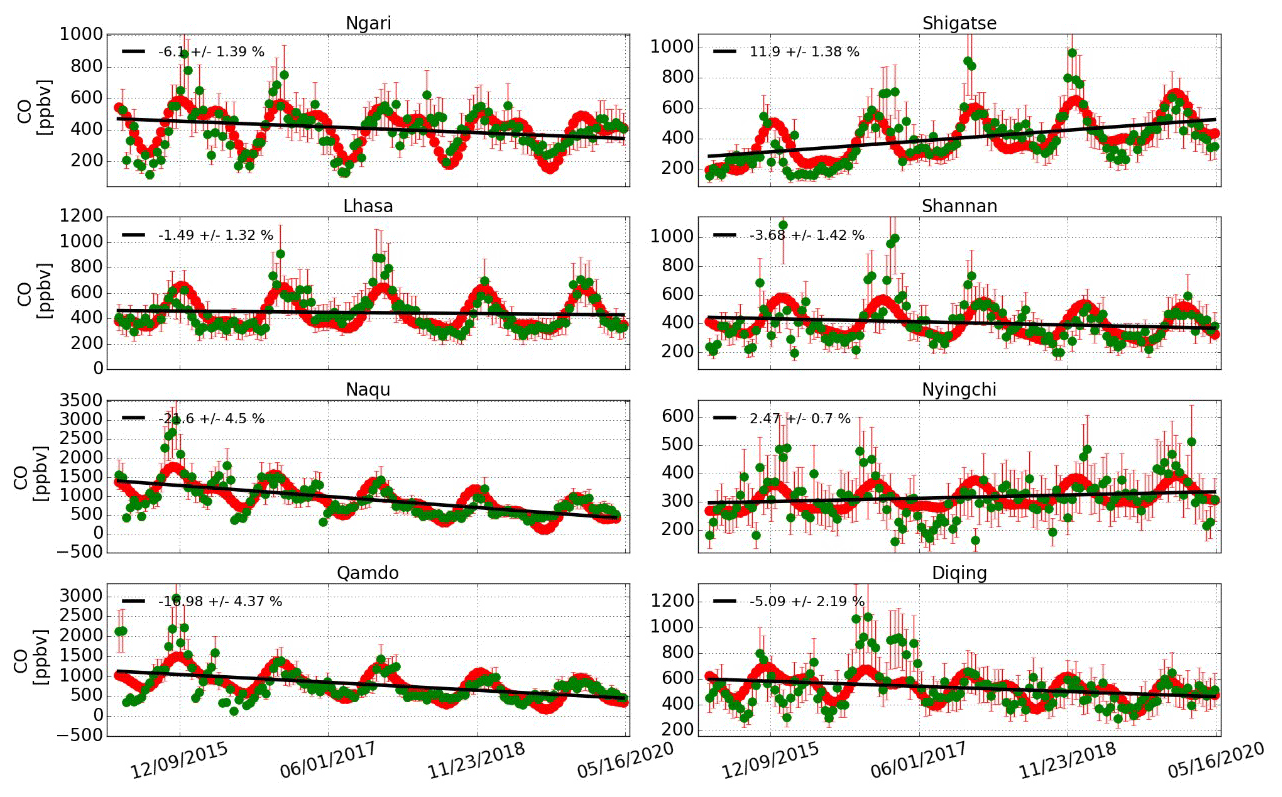
Figure 4 Interannual variabilities of surface CO from 2015 to 2020 over the HTP. Green dots are the biweekly mean of in situ surface CO measurements. Vertical red error bar is 1σ standard variation within the respective 2 weeks. The seasonality and interannual trend in each city fitted by using a bootstrap resampling model with a third Fourier series (red dots) plus a linear function (black line) is also shown.

Surface CO VMR annual mean over the HTP varied over 318.3 ± 71.6 to 901.6 ± 472.2 ppbv depending on year and region (Table 3), where Naqu, Qamdo, and Diqing varied over 531.4 ± 156.8 to 901.6 ± 472.2 ppbv, higher than those in other cities which varied over 318.3 ± 71.6 to 446.1 ± 138.5 ppbv (Table 3). The annual mean concentrations of surface CO over the HTP were compared with those from other cities in China. All cities over the HTP except Naqu and Qamdo can be ranked as a few of the top-level cities with the best air quality. Naqu and Qamdo were ranked as the middle-level cities with fair to poor air quality (http://www.cnemc.cn/en/).

4 Model evaluation over the HTP

The performance of the GEOS-Chem model has been evaluated with available observations over various regions in China and surroundings in previous studies from different perspectives such as surface O₃ concentration in urban regions over China (Lu et al., 2019), tropospheric CO column over eastern China (Chen et al., 2009; Sun et al., 2020) and the Pacific (Yan et al., 2014), tropospheric averaged HCHO concentration over eastern China (Sun et al., 2021), and stratospheric NO₂ partial column (H. Yin et al., 2019) and HCl partial column over eastern China (Yin et al., 2020). Generally, GEOS-Chem is able to reproduce the absolute values as well as seasonal cycles of trace gases over the aforementioned regions. So far GEOS-Chem model evaluation over the complex topography and meteorology of the HTP has not been found in the literature. Here we first use the IASI CO total column from 2015 to 2020 over the HTP to evaluate the model performance in the specifics of the HTP. As the vertical resolution of GEOS-Chem is different from the IASI observation, a smoothing correction was applied to the GEOS-Chem profiles. First, the GEOS-Chem CO profiles were downgraded to the IASI altitude grid to ensure a common altitude grid. Since the IASI overpass time is at about 09:30 LT in the morning, only the GEOS-Chem simulations at 09:00 and 10:00 LT are considered. The interpolated profiles were then smoothed by the monthly mean IASI averaging kernels and a priori profiles (Rodgers, 2000; Rodgers and Connor, 2003). The GEOS-Chem CO total columns were calculated subsequently from the smoothed profiles by using the corresponding regridded air density profiles from the model. Finally, the GEOS-Chem total column time series were averaged by month and compared with the IASI monthly mean data.

Figure 5 Correlation plots of the monthly mean of CO total column over the HTP for GEOS-Chem model simulation against IASI observation. The average for GEOS-Chem simulation is performed at 09:00 and 10:00 LT. The IASI dataset is selected within an ±1^∘ latitude–longitude rectangular area around each city. The blue lines are linear fitted curves of the respective scatter points. The black dotted lines denote one-to-one lines.

Correlation plots for the model-to-IASI data pairs in each region over the HTP are shown in Fig. 5. Depending on regions, the GEOS-Chem simulations over the HTP tend to underestimate the IASI observations by 9.2 % to 20.0 %. The largest GEOS-Chem vs. IASI differences occur in Qamdo and Lhasa, with underestimations of 20.0 % and 18.5 %, respectively. The lowest GEOS-Chem vs. IASI difference occurs in Nyingchi, with an underestimation of 9.2 %. These GEOS-Chem vs. IASI differences over the HTP were mainly attributed to the underestimation of local emission inventories and the coarse spatial resolution of the GEOS-Chem model grid cells. The amount of residential energy use, including fossil fuels and biofuels used for cooking and heating, is not recorded for Tibet in current energy statistics yearbooks; therefore, bottom-up inventories tend to underestimate anthropogenic emissions over the HTP (Zheng et al., 2019). Meanwhile, emissions due to seasonal crop residue burning over the HTP are difficult to quantify accurately (Li et al., 2021). This can be shown by the CO emission distribution over the HTP from the MEIC inventory in Fig. S2, which shows that both the spatial distribution and seasonality of CO emission over the HTP are not in good agreement with the in situ measurements. Besides, the coarse spatial resolution of the GEOS-Chem simulations homogenizes CO concentrations within each 2^∘ × 2.5^∘ model grid cell. The simulation results represent the homogenized concentrations in the grid box at the grid-mean elevation, which could cause significant bias near complex terrain (Yan et al., 2014). Especially the studied regions represent the most developed and populated areas over the HTP, which are surrounded by large areas of rolling mountains with sparsely interspersed farms, pasture, or residency. The horizontal transport and vertical mixing schemes simulated by the GEOS-Chem model at coarse spatial resolutions are difficult to match IASI observation with a ground pixel of a 12 km diameter footprint on the ground at nadir (Clerbaux et al., 2009). Regional difference in CO levels could aggravate the inhomogeneity within the selected GEOS-Chem model grid and thus aggravate the difference between modelled and measured CO concentrations. In addition, the difference between simulation and measurement could also be associated with the uncertainties in meteorological fields, OH fields, and stratosphere–troposphere exchange (STE) scheme over the HTP, which are known issues in the GEOS-Chem model (Bey et al., 2001; Kopacz et al., 2011).

Though not perfect in reproducing the absolute values of the IASI observation, GEOS-Chem can capture the measured seasonal cycle of the CO total column over the HTP with a correlation coefficient (r) of 0.64 to 0.82 depending on regions. In subsequent study, the GEOS-Chem model is used for investigating the influence of long-range transport. We turn off all emission inventories within the HTP in the GEOS-Chem tagged CO simulation and assess the relative contribution of each source and geographical tracer. The relative contribution of each tracer is calculated as the ratio of the corresponding absolute contribution to the modelled total concentration amount. Taking this ratio effectively minimizes the propagation of systematic model errors that are common to all tracers, i.e. the uncertainties in meteorological fields, the vertical mixing and STE schemes, and the mismatch in spatial resolution.

5 Source attribution

5.1 Local emission

The air quality in a city is influenced by local emission, which is spatially differentiated by energy consumption, economic development, industry structure, and population. All the studied cities over the HTP have achieved rapid economic and population growth in recent years (Ran et al., 2014; X. Yin et al., 2019). For example, Lhasa's gross domestic product (GDP) in 2018 was 29 times higher than that of 2001, and the population had increased by more than 230 000 in 17 years (X. Yin et al., 2019). In order to evaluate the influence of local emission, the relationship between in situ measurements of NO₂ and CO is investigated. Correlation plots of surface CO vs. NO₂ daily mean VMR time series provided by the CNEMC network from 2015 to 2020 in eight cities over the HTP are shown in Fig. 6. The results show that NO₂ and CO concentrations were correlated in all cities (r ranges from 0.49 to 0.86) throughout the year. The overall good correlations between these two gas pollutants suggested common sources of ΔNO₂ and ΔCO in these cities. As a short lifetime species (a few hours), the emitted NO₂ is heavily weighted toward the direct vicinity of local emission regions. As a result, local emissions are important sources of CO in all cities. However, the slope ΔNO${}_{\mathrm{2}}/\mathrm{\Delta }$CO (ranges from 0.006 to 0.04) and the degree of the correlation in each city are different, indicating energy consumption and CO emission rates in these cities are different, and additional sources of CO could exist, e.g. from long-range transport or oxidation from CH₄ and NMVOCs originating either nearby or in distant areas.

Figure 6 Correlation plots of surface CO vs. NO₂ VMR daily mean over the HTP. The black line is a linear least-squares fit of the respective data. The linear equation of the fit and the resulting correlation coefficient (r) are shown. Both CO and NO₂ time series are provided by the CNEMC network. Vertical error bar is 1σ standard variation within that day.

The emission from coal burning for heating was thought to be the dominant source of primary gas pollutants in Lhasa in recent years (Ran et al., 2014; X. Yin et al., 2019). A large portion of solely source results in the highest correlation between NO₂ and CO concentrations in Lhasa. In contrast, Qamdo, Naqu, and Diqing are surrounded by alpine farmlands and pastures. Historically, post-harvest crop residue (e.g. highland barley straws and withered grass) was often burned by local farmers to fertilize the soil for the next planting season. As a fine fuel, post-harvest crop residue was often burned directly in the field in large piles and smoulders for weeks. These seasonal crop residue burning behaviours typically occur in the cold season, which could cause a high level of CO emission in this period. Furthermore, local residents extensively use dry yak dung as fuel for cooking or heating throughout the year, which could elevate the background CO level in these regions. As a result, these higher local sources might be an important factor explaining the higher CO magnitude in these regions.

5.2 Long-range transport

Monthly mean contributions of anthropogenic, BB, and oxidation from long-range transport to the surface CO VMR over the HTP are shown in Fig. 7. All statistical results are based on GEOS-Chem tagged CO simulations by turning off the emission inventories within the HTP. Due to the influence of seasonally variable transport and magnitude of the regional emissions, the anthropogenic, BB, and oxidation sources are all seasonal and regionally dependent. Generally, anthropogenic contributions in June–September and DJF are higher than those in the rest of the year. In contrast, high levels of oxidation contribution occur in JJA/SON and low levels of oxidation contribution occur in MAM/DJF. For the BB source, contributions in MAM/DJF are larger than those in JJA/SON. Depending on season and region, relative contributions of anthropogenic, BB, and oxidation transported to the surface CO VMR over the HTP varied over 35 % to 61 %, 5 % to 21 %, and 30 % to 56 %, respectively. The combination of anthropogenic and oxidation sources dominated the contribution, which varied over 80 % to 95 % with an average of 89 % throughout the year.

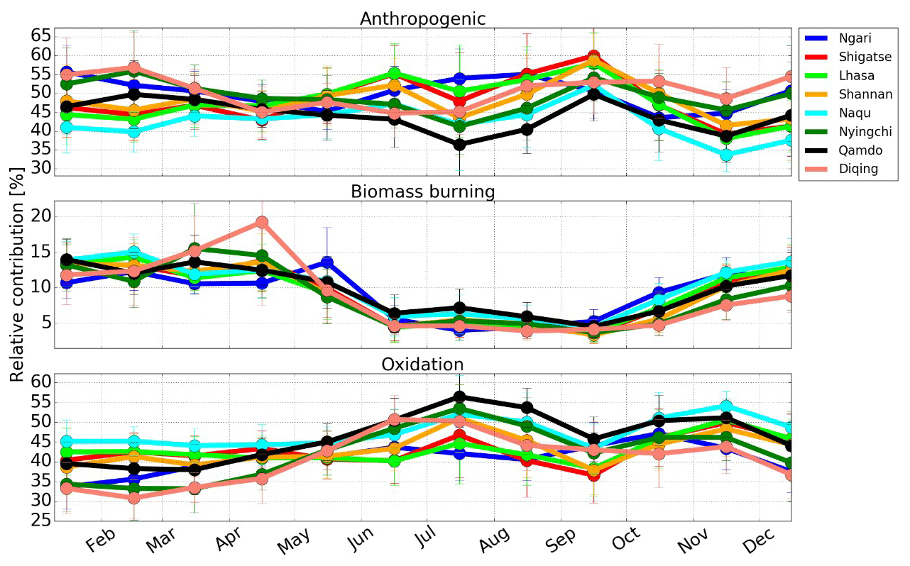
Figure 7 Monthly mean contributions of anthropogenic, biomass burning (BB) and oxidation transport to CO over the HTP. The vertical error bar represents 1σ standard variation within that month. See Table 2 for a description of each tracer.

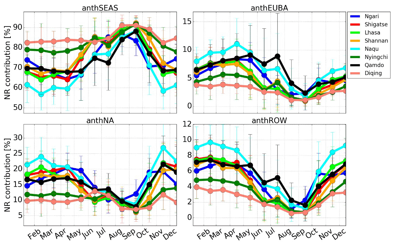
Figure 8 Monthly mean contributions of each geographical anthropogenic tracer to the total anthropogenic-associated CO transport to the HTP. The vertical error bar is the 1σ standard variation within that month. See Table 2 for a description of each tracer.

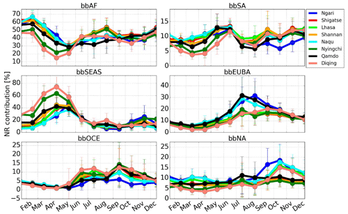
Figure 9 Monthly mean contributions of each geographical BB tracer to the total BB-associated CO transport to the HTP. The vertical error bar represents the 1σ standard variation within that month. See Table 2 for a description of each tracer.

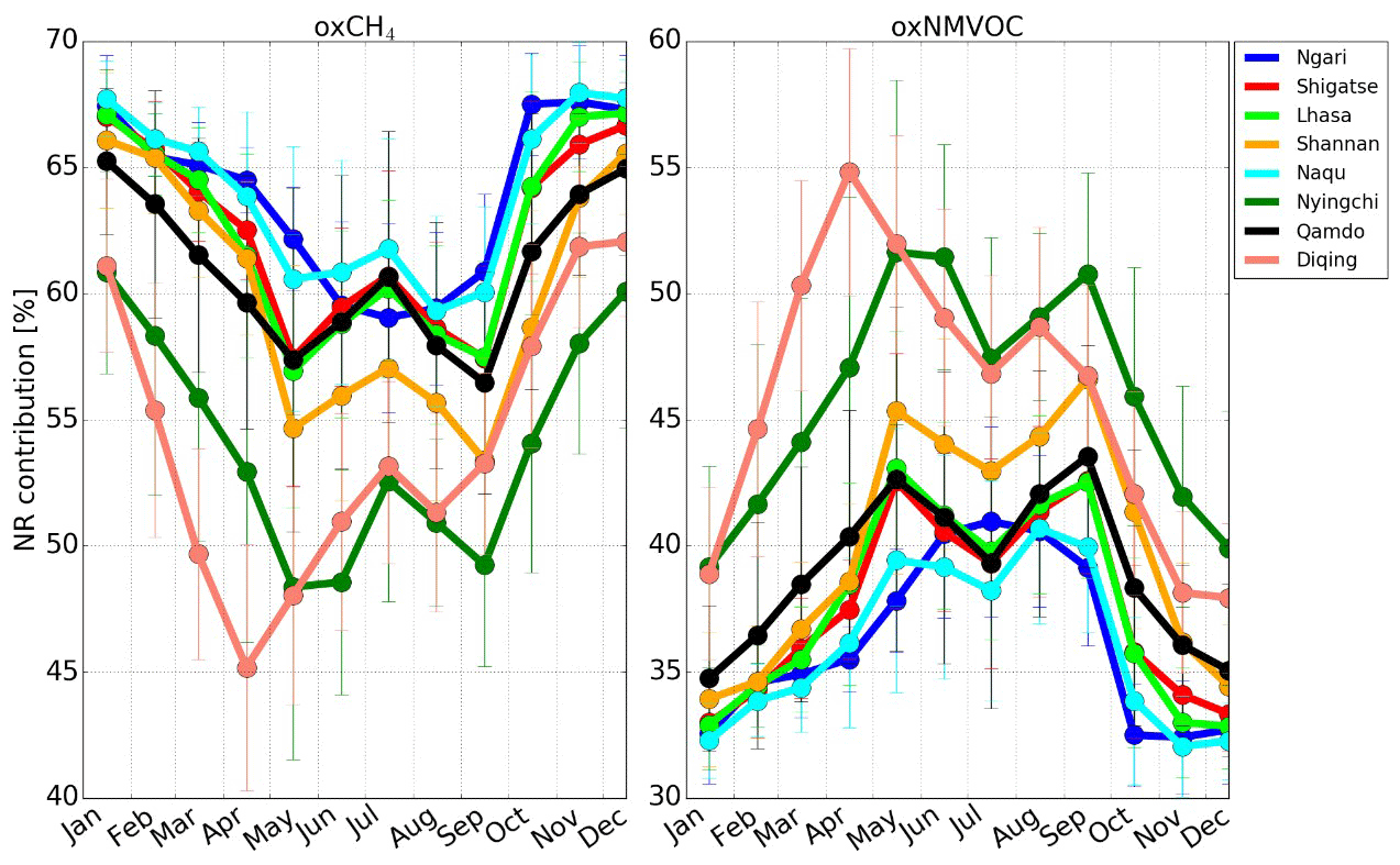
Figure 10 Monthly mean contributions of CH₄ and NMVOC oxidations to the total oxidation-associated CO transport to the HTP. The vertical error bar represents the 1σ standard variation within that month. See Table 2 for a description of each tracer.

After normalizing each regional anthropogenic contribution to the total anthropogenic contribution, the normalized relative (NR) contribution of each anthropogenic region to the total anthropogenic associated transport is obtained in Fig. 8. The results show that the anthropogenic associated transport is mainly attributed to the influence of anthropogenic sources in South Asia and East Asia (SEAS). The NR anthropogenic contribution in SEAS ranges from 58 % in DJF to 91 % in SON. In addition, moderate anthropogenic contributions from North America (NA) (10 % to 27 %), Europe and boreal Asia (EUBA) (4 % to 12 %), and the rest of the world (ROW) (4 % to 10 %) are also observed in MAM/DJF. By using a similar normalized method, the NR contributions of each BB tracer and oxidation tracer are obtained in Figs. 9 and 10, respectively. The results show that large BB contributions are from the Africa (AF) region in July–February (30 %–70 %), the SEAS region in MAM (25 % to 80 %), and the EUBA region in July–September (15 % to 32 %). Additional moderate BB contributions are from the South America (SA) region in May–June and September–December (9 % to 14 %), the Oceania (OCE) region in the second half of the year (5 % to 15 %), and the NA region in September–December (8 % to 19 %). Depending on season and region, 45 % to 67 % of oxidation contribution is attributed to CH₄ oxidation, and 32 % to 55 % of oxidation contribution is attributed to NMVOC oxidation. High-level NR contributions of CH₄ oxidation occur in the cold season (November–March) and low-level NR contributions of CH₄ oxidation occur in the warm season (April–October). The NR contributions of NMVOC oxidation varied over an opposite mode to that of CH₄ oxidation; they maximize in the warm season and minimize in the cold season. The JJA/SON meteorological conditions that show stronger solar radiation, higher temperature, wetter atmospheric condition, and lower pressure than those in DJF/MAM are more favourable for increasing VOC emissions from biogenic sources (BVOCs), which consolidates the fact that contributions of NMVOC oxidation in the warm season are larger than those in the cold season.

By minimizing the propagation of model errors that are common to all tracers (see Sect. 4), the major factors impacting the model interpretation are the uncertainties in emission inventories and OH fields. The uncertainties in CO emission inventories mainly impact primary anthropogenic and BB sources and the uncertainties in CH₄ and VOC emission inventories, and OH fields mainly impact secondary oxidation sources. Additional factors that affect the generation and deplete chemistry of CO or its precursors (e.g. uncertainties in emission inventories of other atmospheric components, stratospheric intrusion of ozone and chemical mechanisms) could also contribute to the uncertainty of the interpretation. All these factors may be seasonal and regionally dependent. A series of GEOS-Chem sensitivity studies might be able to quantify these uncertainties, but this is beyond the scope of the present work.

From Sect. 5.1 and the model interpretation here, we can conclude that the main source of CO in urban areas over the HTP is due to local and SEAS anthropogenic and biomass burning emissions and oxidation sources. In contrast, black carbon in most of the HTP is largely attributed to South-East Asian biomass burning, and locally sourced carbonaceous matter from fossil fuel and biomass combustion also substantially contributes to pollutants in urban cities and some remote regions, respectively (Cong et al., 2007, 2009, 2013; He et al., 2014; Zhang et al., 2015; Zhu et al., 2019; Li et al., 2021; Gul et al., 2021; Thind et al., 2021). Our study emphasized the different origins of diverse atmospheric pollutants in the HTP.

5.3 Transport pathways

The 3D transport trajectories of CO originated in various source regions and sectors to the HTP are identified as below. First, the GEOS-Chem tagged CO simulation is applied for determining the seasonal NR contribution of each tracer (Figs. 8 and 9). For the tracer with a NR contribution of larger than 30 % at a specific time (hereafter enhancement time), the global CO distribution provided by the GEOS-Chem simulation is applied to search for potential CO sources occurring before the enhancement time within 15 d. Then, we generated a series of back trajectories with various travel times to judge whether these CO emissions are capable of travelling to the measurement region. For instance, with respect to each CO enhancement measured at a specific time, we generated 10 back trajectories arriving at 100 m above the ground but with different travel times ranging from 3 to 15 d. If the back trajectories intersect a region where the GEOS-Chem simulation indicates an intensive CO source and the travel duration is within ±2 h of the observed enhancement, then this specific CO source could contribute to the observed enhancement over the HTP. The transport trajectories for this CO source are finally determined. Meanwhile, GEOS-Chem emission inventories are used to classify this CO source into an anthropogenic or BB source. This CO source is regarded as a BB source if the GEOS-Chem BB inventory indicates an intensive CO enhancement. Otherwise, it is regarded as an anthropogenic source.

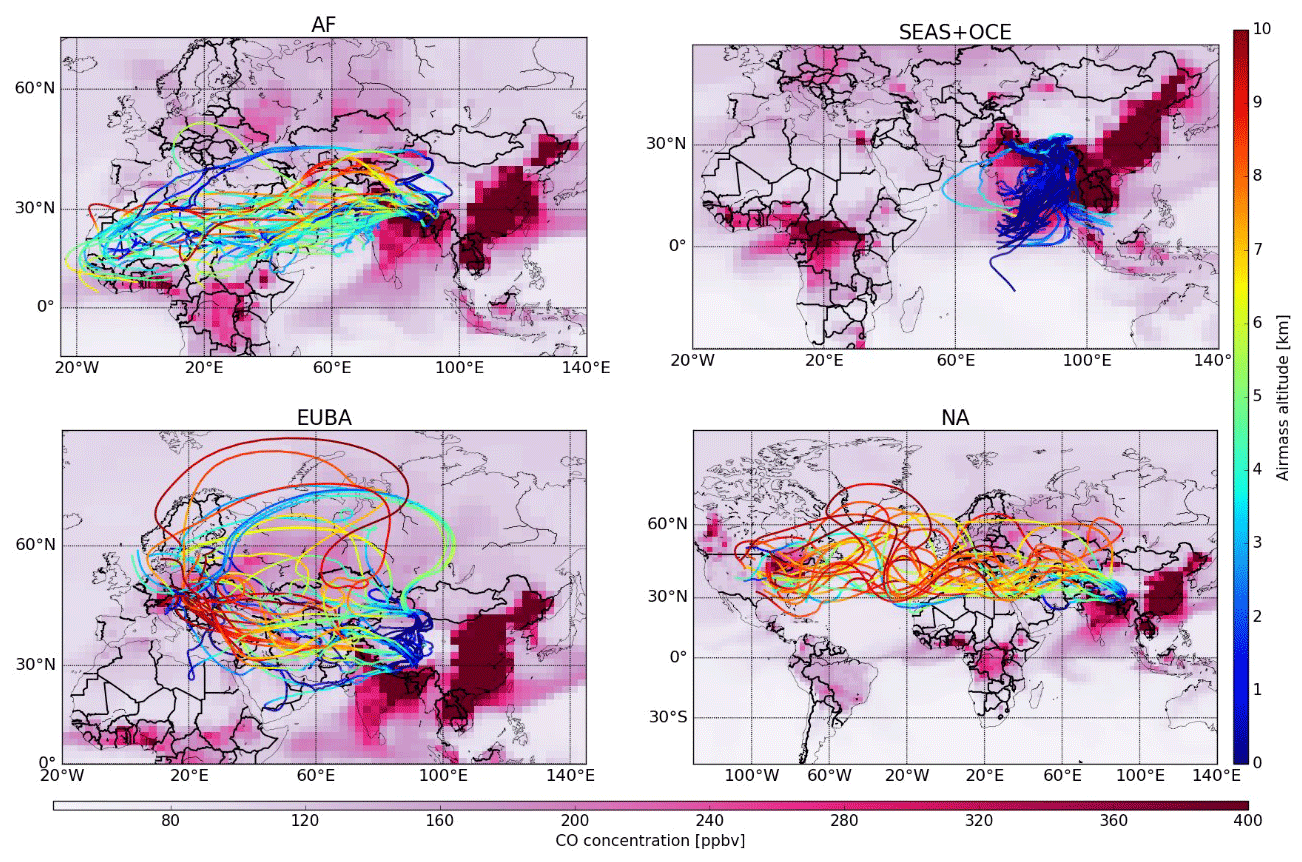
Figure 11 Travel trajectories of polluted air masses originating in AF (SON/DJF), SEAS and OCE (MAM/JJA), EUBA (SON/DJF), and NA (SON/DJF) that reached Naqu (31.5^∘ N) through long-range transport. For clarity, only a few trajectories are selected for demonstration. Travel times are 13, 7, 10, and 14 d, respectively. Global surface CO distributions based on GEOS-Chem simulations are shown for 13, 7, 10, and 14 d prior to the arrival time, respectively. The deeper the colour, the higher the CO concentration.

Figure 12 Spatial distribution of CO VMR in the GEOS-Chem tagged CO simulations in different seasons, and the arrows represent the mean horizontal wind vectors at 500 hPa. The HTP and the studied regions are marked with a blue outline and yellow dots, respectively. Meteorological fields are from the GDAS-1 data.

Figure 11 demonstrates travel trajectories of polluted air masses originating in the AF, SEAS + OCE, EUBA, and NA regions which arrived at Naqu (31.5^∘ N) over the HTP through long-range transport. As the GEOS-Chem BB inventory shows, CO emissions from southern Africa during July–September, central Africa during November–February, central Europe during July–November, Siberia during June–September, and the South Asian peninsula during March–May are dominated by the BB source. Other potential CO sources are dominated by anthropogenic emissions. Figure 12 shows the spatial distribution of CO VMR along with the mean horizontal wind vectors at 500 hPa in different seasons. Figure 13 illustrates the latitude–height and longitude–height distributions of CO VMR along with the 3D atmospheric circulation patterns in different seasons. The 3D transport pathways of CO around the HTP are thus deduced as follows.

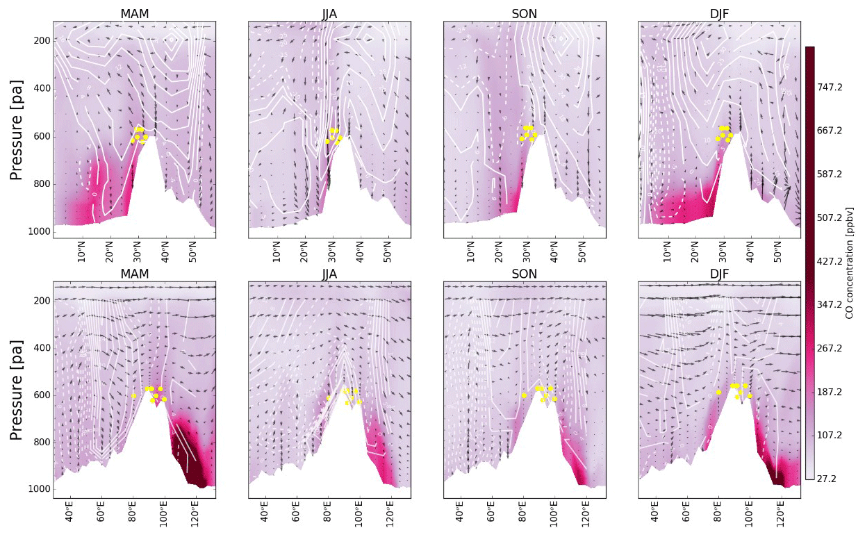
Figure 13 The first row shows the latitude–height distributions of CO VMR averaged over 80–100^∘ E in the tagged CO simulations in different seasons (corresponding to different columns). The white contours at intervals of 6 m s⁻¹ represent the westerly (solid) and easterly (dashed) mean meridional winds; the white area represents topography and the arrows represent the wind vectors (vertical velocity in units of 10⁻⁴ hPa s⁻¹ and zonal wind in m s⁻¹); the studied regions are marked with yellow dots. The second row is similar to the first row except that the quantities are on the longitude–height perspective averaged over 28–33^∘ N. Here the white contours represent the southerly (solid) and northerly (dashed) mean zonal winds, and the horizontal component of the wind vectors is meridional wind (m s⁻¹). Meteorological fields are from the GDAS-1 data.

As indicated by the arrows in Figs. 12 and 13, the strong surface cooling in DJF over the HTP results in divergence and the formation of an enhanced local circulation cell, while in JJA air masses converge toward the HTP from the surroundings triggered by the ascent of strongly heated air masses over the HTP (Zhang et al., 2015). In DJF, the tropical easterlies are weak, but the mid-latitude westerlies extend to the subtropics (∼ 20^∘ N) near the surface and tropics (∼ 10^∘ N) over the middle troposphere (Fig. 13). In the summer monsoon season, the atmospheric circulation patterns around the HTP change dramatically and are dominated by the reversal of the surface wind regime in the tropics, such as the South China Sea, Bay of Bengal, and Arabian Sea (Figs. 11 and 13). Meanwhile, the mid-latitude westerlies in JJA recede to the North Temperate Zone (north of 30^∘ N), and the westerly jet centre shifts to about 40^∘ N (from about 30^∘ N in DJF). In JJA, the tropical region in the south of the HTP is characterized by the strong easterlies in the upper troposphere and by the south-westerly air flow in the lower troposphere (Fig. 13). The prevailing winds during the transition seasons in MAM and SON are still westerlies (Fig. 13). These above-seasonal atmospheric circulation patterns control the CO transport pathway around the HTP. Nevertheless, the transported CO scales to the HTP are also influenced by source location and strength, travel trajectory, and elapsed time (Yao et al., 2012; Zhang et al., 2015; Kang et al., 2019).

In SON/DJF, a significant amount of CO from southern SEAS (anthropogenic source), northern AF (BB source), western EUBA, and northern NA (anthropogenic source) can be transported to the HTP along the westerlies in the dry winter monsoon conditions. CO originating in distant regions such as western EUBA and NA reaches a high altitude (to 8 km) during the transport (Fig. 11). However, CO from the densely populated and industrialized areas in eastern China barely reaches the HTP because of strong removal along the transport pathways to the HTP which circles around the Northern Hemisphere along the westerlies during the winter monsoon season (Fig. 12). In MAM, CO emissions from BB sources in the SEAS region can be transported to the HTP, which is mainly triggered by deep convection followed by northward transport into the mid-latitude westerlies (Liu et al., 2003) (Fig. 13). During the South Asian summer monsoon, the local abundant wet precipitation can remove a large portion of SEAS-originated CO but can still affect the south-western HTP (Fig. 13). Along strong south-easterly air flow in the summer monsoon season, CO from eastern China can be uplifted higher and transported more to the north-eastern HTP than that in the DJF. In addition, large-scale atmospheric deep convection can loft CO from upwind source regions (e.g. central SA and Indonesia, within the OCE region) into higher altitudes, where it can be transported to the HTP in SON or DJF. Generally, CO removals over the HTP in all seasons are driven by atmospheric deep convection which lofts CO into higher altitudes or by westerlies which transport local emissions far away (Fig. 13).

5.4 Factors driving surface CO variability over the HTP

Temporal CO burden is dependent on the difference between the CO source and sink, which is determined by the accumulated influence of local emission, transport, secondary generation, environmental capacity, and OH oxidation capability. The environmental capacity is determined by atmospheric self-clean capability, topography, deposition, and meteorological condition (Hofzumahaus et al., 2009). Atmospheric self-clean capability refers to the capability of the atmosphere in terms of depleting atmospheric pollutants through physical and chemical processes (Rohrer et al., 2014). Generally, the vertical self-clean capability is positively correlated with the PBLH and the horizontal self-clean capability is positively correlated with the wind speed (Rohrer et al., 2014). The OH oxidation capability is positively correlated with temperature, radiation, and OH seasonality (Rohrer et al., 2014).

The bimodal pattern of diurnal cycles for surface CO VMR in urban areas over the HTP is attributed to the following diurnal production and depletion processes. The thin atmosphere over the HTP causes large temperature and radiation differences between day and night (Yin et al., 2017; Kang et al., 2019). The PBLH and OH oxidation capability in the nighttime is much lower than those in the daytime (Ran et al., 2014; Yin et al., 2017; X. Yin et al., 2019). The CO emissions over the HTP start to generate after sunrise and reach the daytime maximum during rush hours at 08:00 to 11:00 LT in the morning. The CO concentration is then decreasing as a result of depletion by reactions with OH to form O₃ or transport far away (Ran et al., 2014; X. Yin et al., 2019). Subsequently, CO emissions start to generate again during rush hours at 16:00 to 19:00 LT in the afternoon and reach the nighttime maximum at 21:00 to 23:00 LT due to low PBLH and OH oxidation capability in the nighttime (Ran et al., 2014; X. Yin et al., 2019).

Similarly, the seasonal cycle of surface CO VMR in the urban areas over the HTP is determined by the seasonal variability of CO source, environmental capacity, and OH oxidation capability. High levels of surface CO VMR in the late autumn to spring can be attributed to low PBLH and OH oxidation capability but high local and transported CO in the period and vice versa for low levels of surface CO VMR in summer to early autumn (X. Yin et al., 2019). Specifically, local anthropogenic CO sources (mainly heating activities) and crop residue burning behaviours in urban regions over the HTP during the colder post-monsoon and winter months are higher than those in other seasons. Meanwhile, the westerlies near the surface in SON/DJF are weaker than those in MAM/JJA, which facilitates the accumulation of atmospheric pollutants (Fig. 13). Furthermore, high levels of CO are observed in the late autumn to spring in neighbouring SEAS countries due to intensive anthropogenic emissions or BB practices (Kan et al., 2012; Tiwari et al., 2014; Liu et al., 2018; Gani et al., 2019). These polluted air masses can transport to the HTP region and elevate the local CO level (Fig. 13). Thus, apart from local anthropogenic and BB emissions, these transported sources might be an important factor explaining the high CO pollution in winter.

Since the crop residue burning emissions result in poor air quality that threatens local terrestrial ecosystems and human health, the Chinese government started to ban crop residue burning over China since 2015, and henceforth the crop residue burning events over the HTP decreased dramatically (Sun et al., 2020) (http://www.chinalaw.gov.cn, last access: 19 June 2020). Meanwhile, the major air pollutant emissions have decreased around the globe in recent years as a consequence of active clean air policies for mitigating severe air pollution problems in the major anthropogenic emission regions, such as China, India, Europe, and North America (Zheng et al., 2018; Sun et al., 2021). Furthermore, elevated BB events in the AF, SEAS, and OCE regions were observed at the beginning of the studied years due to the El Niño–Southern Oscillation (ENSO) in 2015 (Sun et al., 2020). All these factors probably drive a decreasing trend in surface CO VMR since 2015 in most cities over the HTP. However, an overall increase in surface CO VMR in Shigatse and Nyingchi since 2015 indicated that the decrease in transported CO was overwhelmed by the increase in local CO emissions as a result of the expansion of urbanization, industrialization, land use, and infrastructure construction near the two cities.

6 Conclusions

In this study, we quantified the variability, source, and transport of CO in the urban areas over the Himalayas and Tibetan Plateau (HTP) by using in situ measurement, GEOS-Chem model tagged CO simulation, and the analysis of meteorological fields. Diurnal, seasonal, and interannual variabilities of CO over the HTP are investigated with ∼ 6 years (January 2015 to July 2020) of surface CO measurements in eight cities over the HTP. Annual mean of surface CO volume mixing ratio (VMR) over the HTP varied over 318.3 ± 71.6 to 901.6 ± 472.2 ppbv, and a large seasonal cycle was observed with high levels of CO VMR in the late autumn to spring and low levels of VMR in summer to early autumn. Surface CO VMR burdens and variations in Naqu, Qamdo, and Diqing are higher than those in other cities in all seasons. The diurnal cycle is characterized by a bimodal pattern with two maximums occurring around 09:00 to 11:00 LT in the daytime and 21:00 to 23:00 LT in the nighttime. The trend in surface CO VMR from 2015 to 2020 over the HTP spanned a large range of (−21.6 ± 4.5) % yr⁻¹ to (11.9 ± 1.38) % yr⁻¹, indicating a regional representation of each dataset. However, surface CO VMR from 2015 to 2020 in most cities over the HTP showed negative trends.

The IASI satellite observations are for the first time used to assess the performance of the GEOS-Chem full-chemistry model for the specifics of topography and meteorology over the HTP. Depending on the region, the GEOS-Chem simulations over the HTP tend to underestimate the IASI observations by 9.2 % to 20.0 %. Though not perfect in reproducing the absolute values of the IASI observation, GEOS-Chem can capture the measured seasonal cycle of the CO total column over the HTP with a correlation coefficient (r) of 0.64 to 0.82 depending on regions. Distinct dependencies of CO on a short-lifetime species of NO₂ in almost all cities over the HTP were observed, implying local emissions to be predominant. By turning off the emission inventories within the HTP in GEOS-Chem tagged CO simulation, the relative contribution of long-range transport was evaluated. The results showed that transport ratios of primary anthropogenic source, primary biomass burning (BB) source, and secondary oxidation source to the surface CO VMR over the HTP varied over 35 % to 61 %, 5 % to 21 %, and 30 % to 56 %, respectively. The anthropogenic contribution is dominated by the South Asia and East Asia (SEAS) region throughout the year (58 % to 91 %). The BB contribution is dominated by the SEAS region in spring (25 % to 80 %) and the Africa (AF) region in July–February (30 %–70 %). Additional important anthropogenic contributions from North America (NA) (10 % to 27 %) and Europe and boreal Asia (EUBA) (4 % to 12 %) in spring and winter (MAM/DJF) are also observed. Additional important BB contributions are from the EUBA region in July–September (15 % to 32 %), the South America (SA) region in May–June and September–December (9 % to 14 %), the Oceania (OCE) region in the second half of the year (5 % to 15 %), and the NA region in September–December (8 % to 19 %). The decreasing trends in surface CO VMR since 2015 in most cities over the HTP are attributed to the reduction in local and transported CO emissions in recent years.

This study concluded that the main source of CO in urban areas over the HTP is due to local and SEAS anthropogenic and BB emissions and oxidation sources. In contrast, black carbon in most of the HTP is largely attributed to South-East Asian biomass burning, and locally sourced carbonaceous matter from fossil fuel and biomass combustion also substantially contributes to pollutants in urban cities and some remote regions, respectively. This study not only emphasized the different origins of diverse atmospheric pollutants in the HTP, but also improved knowledge of the variabilities, sources, drivers, and transport pathways of atmospheric pollutants over the HTP and provided guidance for potential regulatory and control actions.