Estimating Upper Silesian coal mine methane emissions from airborne in situ observations and dispersion modeling

Abundant mining and industrial activities located in the Upper Silesian Coal Basin (USCB) lead to large emissions of the potent greenhouse gas (GHG) methane (CH₄). The strong localization of CH₄ emitters (mostly confined to known coal mine ventilation shafts) and the large emissions of 448 and 720 kt CH₄ yr⁻¹ reported in the European Pollutant Release and Transfer Register (E-PRTR 2017) and the Emissions Database for Global Atmospheric Research (EDGAR v4.3.2), respectively, make the USCB a prime research target for validating and improving CH₄ flux estimation techniques. High-precision observations of this GHG were made downwind of local (e.g., single facilities) to regional-scale (e.g., agglomerations) sources in the context of the CoMet 1.0 campaign in early summer 2018. A quantum cascade–interband cascade laser (QCL–ICL)-based spectrometer adapted for airborne research was deployed aboard the German Aerospace Center (DLR) Cessna 208B to sample the planetary boundary layer (PBL) in situ. Regional CH₄ emission estimates for the USCB are derived using a model approach including assimilated wind soundings from three ground-based Doppler lidars. Although retrieving estimates for individual emitters is difficult using only single flights due to sparse data availability, the combination of two flights allows for exploiting different meteorological conditions (analogous to a sparse tomography algorithm) to establish confidence on facility-level estimates. Emission rates from individual sources not only are needed for unambiguous comparisons between bottom-up and top-down inventories but also become indispensable if (independently verifiable) sanctions are to be imposed on individual companies emitting GHGs. An uncertainty analysis is presented for both the regional-scale and facility-level emission estimates. We find instantaneous coal mine emission estimates of 451/423 ± 77$/$79 kt CH₄ yr⁻¹ for the morning/afternoon flight of 6 June 2018. The derived fuel-exploitation emission rates coincide (±6 %) with annual-average inventorial data from E-PRTR 2017 although they are distinctly lower (−28 %/−32 %) than values reported in EDGAR v4.3.2. Discrepancies in available emission inventories could potentially be narrowed down with sufficient observations using the method described herein to bridge the gap between instantaneous emission estimates and yearly averaged inventories.

1 Introduction

The growth in population and economy since the pre-industrial era has been going hand in hand with rising anthropogenic emissions, causing a strong increase in atmospheric greenhouse gas (GHG) concentrations. This is in general attributed to anthropogenic emissions from a large variety of sources omnipresent in modern life (Pachauri et al., 2014), e.g., extraction, processing, and transport of fossil fuels. Despite the evident anthropogenic influence on the climate in general, large uncertainties remain in the magnitude of human-induced radiative forcing and relative contributions from different sectors (Nisbet et al., 2014; Kirschke et al., 2013). Approximately 20 % of the global CH₄ source is estimated to arise from the sector of fossil fuel industry (Schwietzke et al., 2016), which also includes activities like coal mining – an industry for which the Upper Silesian Coal Basin (USCB), located in southern Poland and the Czech Republic, is well known.

According to the European Pollutant Release and Transfer Register (E-PRTR 2017; https://prtr.eea.europa.eu/, last access: 6 May 2020) a total of 448 kt CH₄ yr⁻¹ is emitted into the air from the USCB region, making it one of Europe's methane emission hot spots. The intensive mining activities and the heavy industry spread around the city of Katowice lead to these significant amounts of CH₄ emitted into the atmosphere, where over 99 % of the CH₄ emissions reported in E-PRTR 2017, listing emitters above a threshold of 0.1 kt CH₄ yr⁻¹, are attributed to mining and related industry. These large emissions are also apparent in the Emissions Database for Global Atmospheric Research (EDGAR v4.3.2) emission inventory reporting a total of 720 kt CH₄ yr⁻¹ in 2012.

The design and subsequent control of mitigation measures to slow down the increase in atmospheric GHG concentrations require reliable verification and attribution of GHG emissions now and in the future. An established method to derive GHG emissions is known as the top-down approach. This method is based on observed GHG concentrations in the atmosphere and projects their variations (both in time and space) back onto the emissions that may have caused these variations (Nisbet and Weiss, 2010; Chevallier et al., 2005; Peters et al., 2007). For CH₄, concentrations downwind of local- to regional-scale emission sources can be sampled efficiently using high-precision airborne measurements within the planetary boundary layer (PBL). Onboard meteorological instrumentation allows for concurrent sensing of important atmospheric state variables like static pressure and air temperature, as well as the local wind field, which are particularly useful to estimate emissions. In situ instruments provide point measurements at high precision that can be used well for flux estimation using techniques like the mass balance approach (Karion et al., 2013; Conley et al., 2017; Pitt et al., 2019). Previous studies used airborne in situ instrumentation to estimate regional CH₄ emissions from oil and natural gas operations in the USA and Canada (Johnson et al., 2017; Karion et al., 2015; Barkley et al., 2017). These studies find emission inventories (EDGAR) to underestimate CH₄ emissions from the respective sector. Recent studies have also targeted urban CH₄ emissions (Ryoo et al., 2019; Plant et al., 2019; Ren et al., 2018) and anthropogenic CH₄ emissions from agriculture and waste treatment (Yu et al., 2020). Airborne in situ data have further been used to estimate emissions on a facility level by flying closed circles around individual emitters (Lavoie et al., 2015; Conley et al., 2017; Hajny et al., 2019; Mehrotra et al., 2017; Baray et al., 2018).

Recently, Luther et al. (2019) reported on XCH4 flux estimates ranging from 6 ± 1 kt CH₄ yr⁻¹ for single shafts to up to 109 ± 33 kt CH₄ yr⁻¹ for a subregion of the USCB from ground-based, portable, sun-viewing Fourier transform spectrometers mounted on a truck. Fiehn et al. (2020) investigated CH₄ emissions from the USCB using a mass balance approach. They report emission estimates of 436 ± 115 and 477 ± 101 kt CH₄ yr⁻¹ from two research flights along with a detailed uncertainty analysis. The present study is based on the very same research flights and aims at contributing an advanced model approach. Previous studies have used Lagrangian models to simulate the dispersion (Tuccella et al., 2017; Raut et al., 2017) of plumes emanating from oil and gas platforms or identification of CH₄ sources (Platt et al., 2018). Atmospheric transport models have been used to infer CH₄ emissions from the oil and natural gas industry (Barkley et al., 2017). Here, a combination of an Eulerian atmospheric transport model and a Lagrangian particle dispersion model is used in conjunction with assimilated Doppler lidar soundings to infer instantaneous CH₄ emissions for Europe's largest coal extraction region, the USCB.

Section 2 provides an introduction to the USCB as the region of prime interest followed by a research flight overview in Sect. 3. Section 4 details a model-based flux estimation approach. CH₄ emission estimates will be given in the form of a case study in Sect. 4.1 for two research flights on 6 June 2018 along with an estimate of the uncertainties involved. Section 5 summarizes our findings and concludes the study.

2 The Upper Silesian Coal Basin

The Upper Silesian Coal Basin is a plateau elevated between 200 and 300 m above sea level (a.s.l.) in southern Poland. To the south it is confined by the Tatra Mountains reaching up to 2655 m a.s.l. and forming a natural border between Slovakia and Poland. To the west it extends across the national border between Poland and the Czech Republic into the Ostrava region.

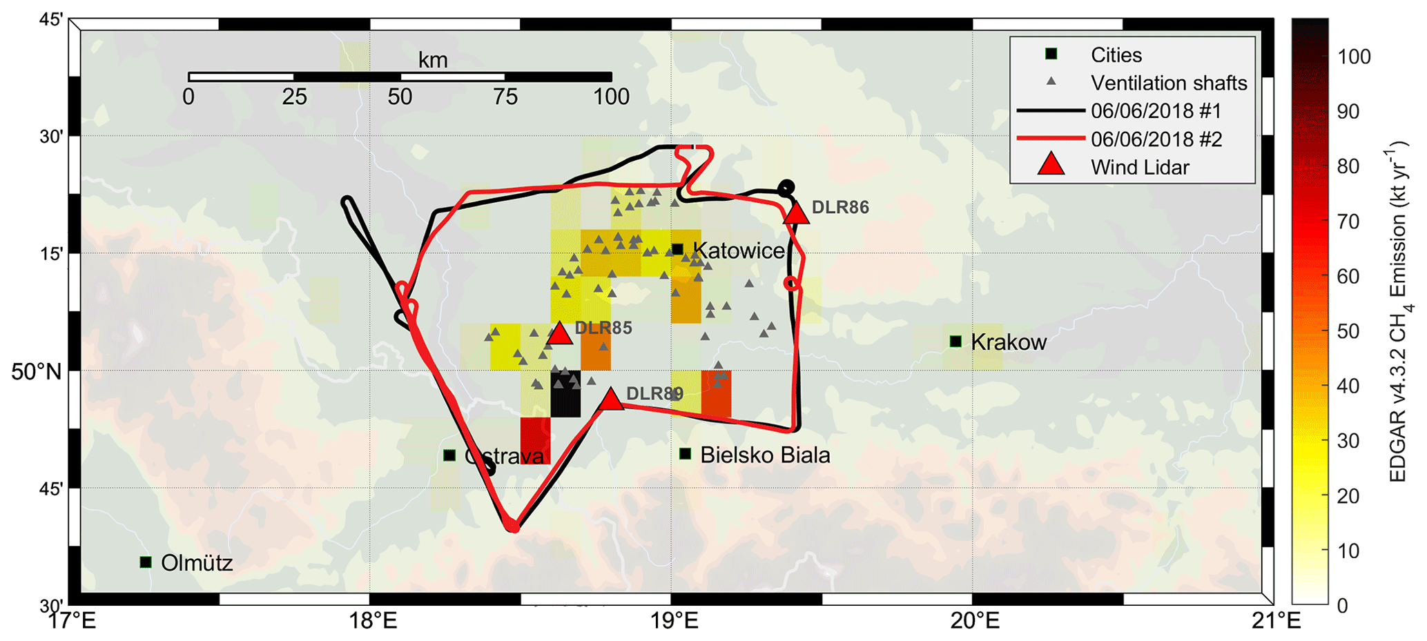
Figure 1 Flight trajectories of two flights of the German Aerospace Center (DLR) Cessna 208B sampling the USCB area during the CoMet field campaign. The plot shows flight trajectories for the morning flight (black) and afternoon flight (red) on 6 June 2018. Red triangles mark the location of three Doppler wind lidars, deployed in the USCB area during the CoMet campaign. Gray triangles mark known coal mine ventilation shafts. Colored tiles are from the EDGAR v4.3.2 CH₄ emission inventory for 2012, showing typical emissions ranging up to ∼ 100 kt yr⁻¹.

According to Gzyl et al. (2017), the USCB is well known for its abundant mining and industrial activities, including coal, zinc, and lead ore exploitation. Coal mining activities make up the largest part, with an approximate total of 10×10⁹ t extracted since the industrial revolution, where over 70 % of this exploitation took place after 1945. To date an approximate 75×10⁶ t of coal is extracted every year from 27 active mines. It is these figures and the large area of approximately 7400 km² covered that make the USCB the largest coal extraction region in Europe (Dulias, 2016). The intensive coal mining activities and the heavy industry spread around the city of Katowice, Poland, located in the north of the USCB, lead to significant amounts of GHG emissions in this area. Fugitive CH₄ emanating from the coal mine shafts reaching several hundred meters into the ground is either actively ventilated (active mines) or degasses passively from abandoned mines. Mines located in the north of the USCB are mostly abandoned and partially flooded, while intensive, active coal exploitation is located in the southern USCB, in both Poland and the Czech Republic (Gzyl et al., 2017).

Global emission inventories show large sources of methane in this area as depicted by the colored tiles in Fig. 1. The figure is based on a subset of the publicly available EDGAR v4.3.2 CH₄ (https://edgar.jrc.ec.europa.eu/, last access” 6 May 2020) emission inventory (Janssens-Maenhout et al., 2017). It shows CH₄ emissions range up to approx. 100 kt yr⁻¹ on a 0.1^∘  × 0.1^∘ grid with source strengths increasing towards the southern USCB. Accordingly, the strongest sources are located near the Czech border midway between the cities of Bielsko-Biała, Poland, and Ostrava, Czech Republic.

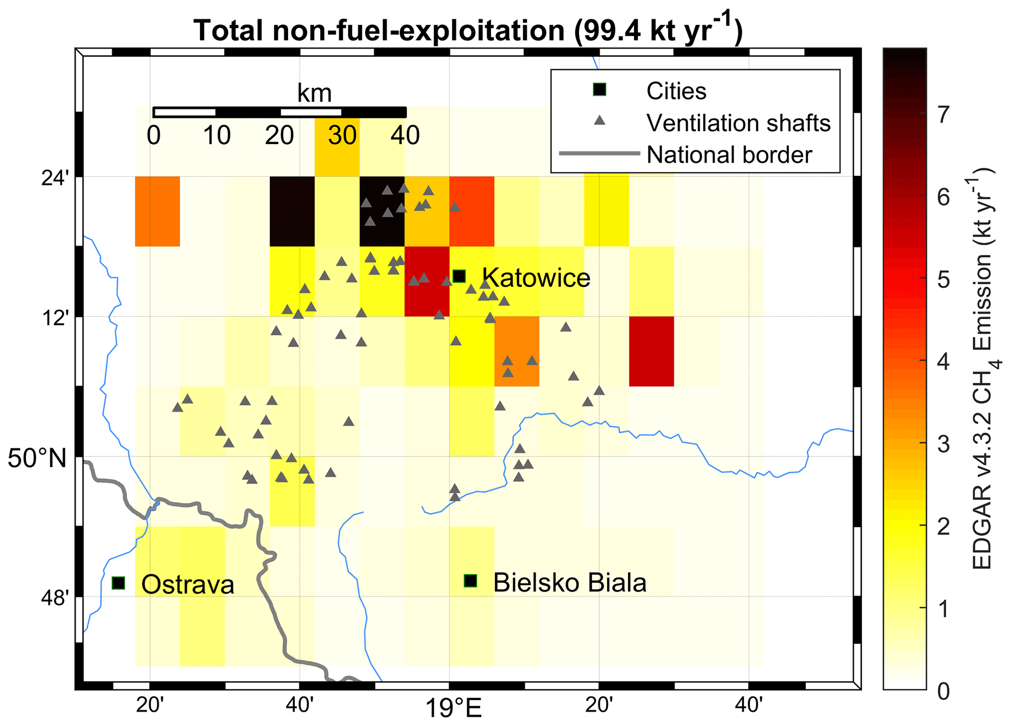
Figure 2 Total non-fuel-exploitation CH₄ emission from the EDGAR v4.3.2 emission inventory corresponding to the following five sectors: solid waste landfills, energy for buildings, waste water handling, enteric fermentation, and oil refineries and transformation energy.

According to EDGAR v4.3.2, these CH₄ sources are among the strongest in Europe. The total CH₄ emissions from this inventory amount to approximately 720 kt yr⁻¹ for the USCB region, where ∼ 620 kt yr⁻¹ is attributed to the fuel-exploitation sector. The EDGAR v4.3.2 inventory further includes information on sectorial partitioning of the remaining non-fuel-exploitation CH₄ emissions making up for approximately 14 % of total annual CH₄ emissions in the USCB. From these ∼ 14 % approximately 90 % are attributed to the following five sectors: solid waste landfills, energy for buildings, waste water handling, enteric fermentation, and oil refineries and transformation energy. The spatial distribution of the total non-fuel-exploitation CH₄ emissions from these five sectors is shown in Fig. 2. Most emitters are weak in comparison to fuel exploitation and uniformly distributed and will be canceled out by the later-described background subtraction. We added stronger source tiles (threshold ≥ 4 kt yr⁻¹) emitting a total of 33 kt yr⁻¹ to our FLEXPART-WRF (FLEXible PARTicle dispersion model–Weather Research and Forecasting) simulation. Facility-level emission data of CH₄ are provided by E-PRTR 2017. The locations of 74 documented coal mine ventilation shafts (active and inactive) have been added to Fig. 1 for reference. These locations were visually identified from satellite imagery, and emission values from E-PRTR 2017 were evenly distributed among the ventilation shafts for each company (see also Nickl et al., 2020). According to E-PRTR 2017, individual contributions sum to a total CH₄ emission of approximately 448 kt yr⁻¹. This value is approximately 38 % lower compared to the EDGAR v4.3.2 inventory (28 % if only considering the fuel-exploitation sector), showing the large uncertainties present in the available data.

3 Research flight overview

The CoMet mission in early summer 2018 primarily aimed at providing observations of GHG (mainly CO₂ and CH₄) gradients along large-scale latitudinal transects over Europe from the coordinated operation of several state-of-the-art instruments on the ground and aboard five research aircraft. Aboard the Cessna 208B, a rich dataset of simultaneous airborne observations of CH₄, C₂H₆, CO₂, CO, N₂O, and H₂O was collected using the quantum cascade laser spectrometer (QCLS) instrument (see Fig. 3 and Kostinek et al., 2019, for details) during ∼30 flight hours. In the following, a subset of these data from two research flights undertaken on 6 June 2018 was used to retrieve CH₄ fluxes emanating from the USCB region. Both flight tracks are shown in Fig. 1 along with the locations of three co-deployed Leosphere Windcube 200S Doppler wind lidars (Wildmann et al., 2020). The morning (black line) and afternoon (red line) flights circumvent all known ventilation shafts in the area (gray triangles) and are in fact very similar (congruent) from the top-down perspective. This is intended to enhance confidence in retrieved GHG fluxes. Moderate (3–6 m s⁻¹) winds throughout the day from northeasterly directions drive advection of the CH₄ plumes towards the Czech border and into the Ostrava region.

The morning flight (black line in Fig. 1) on 6 June 2018 starts off from Katowice Airport, located to the north of the city center, at around 09:15 UTC. Following a short constant-altitude transect, a spiral-up was flown in the east to obtain a sounding out of the boundary layer. This maneuver, revealing a boundary layer depth of approximately 1150 m above mean sea level (a.m.s.l.), was followed by an upwind leg flown at a constant altitude of 900 $\mathrm{m}\mathrm{a}.\mathrm{m}.\mathrm{s}.\mathrm{l}.$ showing a fairly homogeneous CH₄ inflow into the area of interest, thus allowing for subtracting an out-of-plume background (as described in Sect. 4.4) from the measured mole fractions downwind of the mines. Mixing ratios decreased slightly towards free tropospheric background values when climbing above the PBL. Before returning back to Katowice Airport at around 11:45 UTC, the downwind wall maneuver, consisting of five constant-altitude flight legs to the west, was performed at altitudes of approximately 800 m, 1.1 km, 950 m, 1.4 km, and 1.8 $\mathrm{km}\mathrm{a}.\mathrm{m}.\mathrm{s}.\mathrm{l}.$. During the last two flight legs, the aircraft was outside of the PBL.

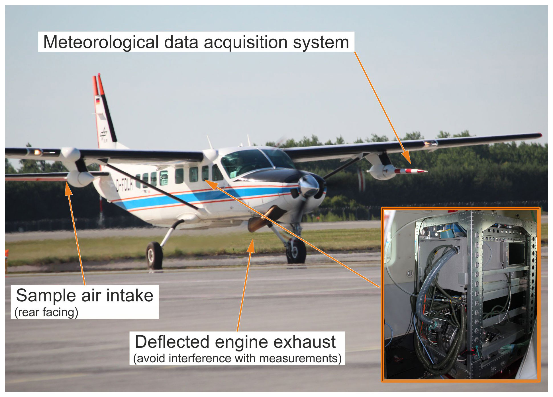
Figure 3 The DLR Cessna 208B on the taxiway at Katowice Airport. The sample air intake is mounted underneath the right wing. The meteorological data acquisition system is underneath the left wing. The QCLS instrument (lower right panel) is located inside the cabin behind the pilot seats.

The afternoon flight (red line in Fig. 1) started off from Katowice Airport around 13:15 UTC. An upwind leg flown at a constant altitude of 900 $\mathrm{m}\mathrm{a}.\mathrm{m}.\mathrm{s}.\mathrm{l}.$ again showed a fairly homogeneous CH₄ inflow into the USCB area. Mixing ratios decrease slightly towards free tropospheric background values when climbing above the PBL during a climb and descent maneuver flown parallel to the sensed mean wind direction. During this flight, we observed a latitudinally inclined PBL with an approximate depth of 1.7 $\mathrm{km}\mathrm{a}.\mathrm{m}.\mathrm{s}.\mathrm{l}.$ in the northern section and 1.3 $\mathrm{km}\mathrm{a}.\mathrm{m}.\mathrm{s}.\mathrm{l}.$ towards the south. Before returning back to Katowice Airport at around 15:30 UTC, the downwind wall maneuver, consisting of six constant-altitude flight legs, was performed over the western USCB region at altitudes of approximately 800 m, 890 m, 975 m, 950 m, 1.1 km, 1.5 km, and 1.8 $\mathrm{km}\mathrm{a}.\mathrm{m}.\mathrm{s}.\mathrm{l}.$.

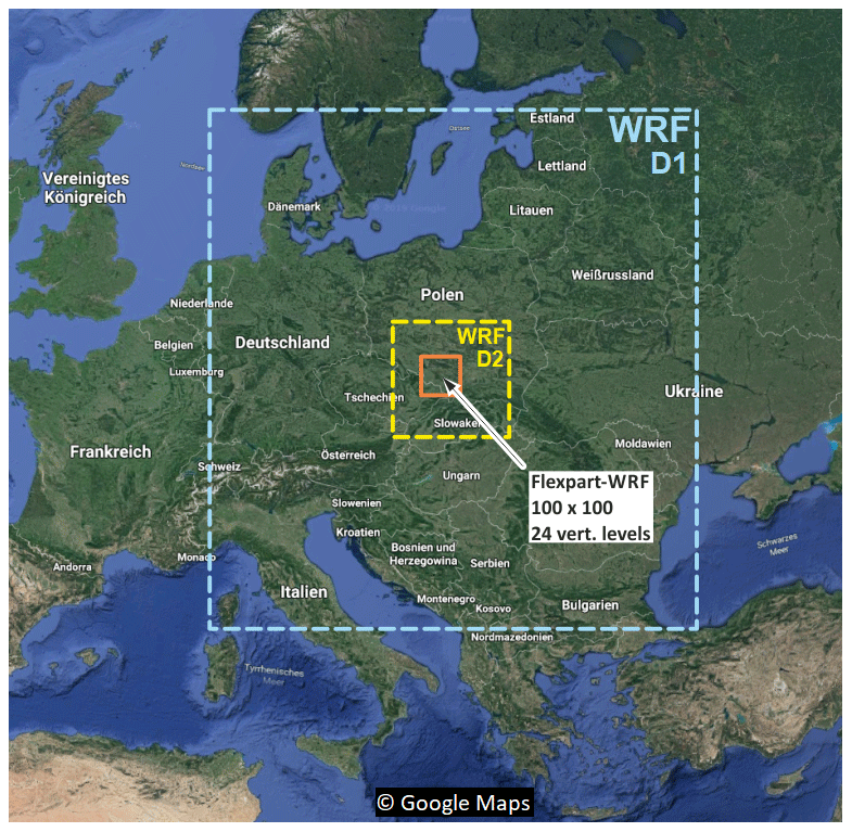
Figure 4 The FLEXPART-WRF domain resides in the nested WRF domain D2 providing the meteorological driver data. Generous spacing towards the driver domain has been included to avoid spurious boundary effects.

4 Estimating emissions

The model-based approach developed in this work employs a combination of Eulerian and Lagrangian particle dispersion models. Due to the known locations of the coal mine ventilation shafts, their emissions are modeled forward in time with constant emission rates. Modeled data are then extracted at the aircraft position in space and time and compared to actual airborne in situ observations. This comparison depends on the quality of the a priori emission data, the quality of the measurements, and the quality of the transport model simulation, which in turn depends on the quality of the meteorological data (winds, PBL heights, etc.). Validating the meteorological data is therefore important to enable regional emission estimates based on particle dispersion models. Here, meteorological driver data are generated using the Weather Research and Forecasting (WRF) v4.0 model (Powers et al., 2017) with assimilated soundings from three Leosphere Windcube 200S Doppler wind lidars. Data are then fed into the Lagrangian particle dispersion model FLEXPART-WRF – a FLEXPART (Pisso et al., 2019) version adapted for WRF meteorology – and used to model the exhaust plumes emanating from ventilation shafts of the emitters listed in E-PRTR 2017.

4.1 Local-scale meteorology using WRF

Figure 4 shows a satellite map of central Europe with the two domains specified for the USCB region. The outer domain D1 (light blue box in Fig. 4) with a horizontal grid resolution of ∼15 km includes large parts of central Europe.

This domain is fed by NCEP GDAS/FNL Operational Global Analysis data on a $\mathrm{0.25}{}^{\circ }\times \mathrm{0.25}$^∘ grid, available from the NCAR–UCAR Research Data Archive at a 3 h time resolution (National Centers for Environmental Prediction/National Weather Service/NOAA/U.S. Department of Commerce, 2015). The grid four-dimensional data assimilation (GFDDA) module is used to nudge modeled meteorology towards the analysis data at each grid point. The outer domain is intended to catch the large-scale weather situation over Europe and to provide a smooth transition between the coarse NCEP GDAS/FNL Operational Global Analysis and the region of prime interest. The inner domain D2 (yellow box in Fig. 4) has a horizontal grid resolution of ∼3 km and covers the entire USCB region. The model output from D2 is the primary product required for subsequent FLEXPART runs. Both domains are driven with the original WRF v4.0 topographic data with a resolution of 30 arcsec. Vertically, the model atmosphere is divided into 33 stacked layers, with the top layer at 200 hPa (corresponding to approximately 12 km in altitude). Vertical layers are more closely spaced at lower altitudes to enable a better resolution of boundary layer processes. The modeled atmospheric state variables are output every hour for D1 and every 5 min for D2.

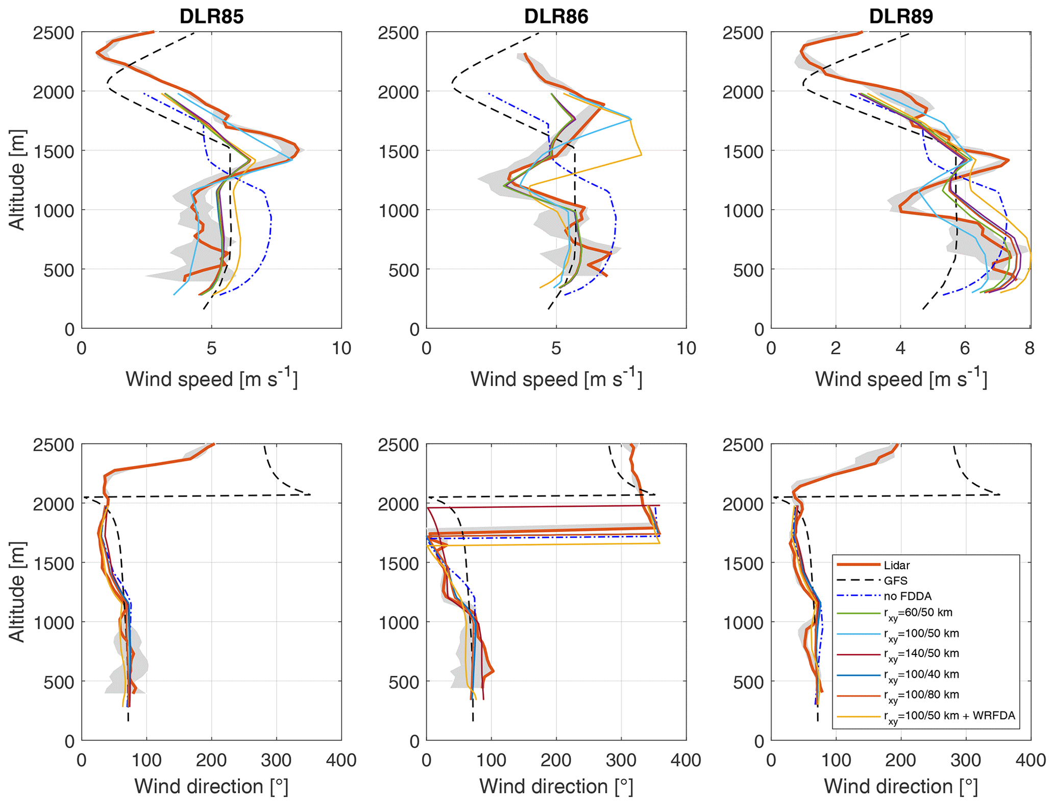
Figure 5 Ensemble WRF runs with varying radii of influence r_xy in comparison to interpolated NCEP GDAS/FNL and actual lidar soundings for 6 June 2018 at 09:00 UTC. The shaded area shows the maximum variability including soundings timed 20 min before and 20 min after the observations used. Abscissa units are m s⁻¹ and degrees.

Soundings from three Doppler lidars (marked DLR85, DLR86, and DLR89) deployed in the USCB area during the CoMet mission (see Fig. 1 for respective positions) have been used to augment the model output (Wildmann et al., 2020). These data are available on a regular, continuous basis throughout the campaign period at 10 min time intervals with soundings typically reaching up to ∼ 2.5 $\mathrm{km}\mathrm{a}.\mathrm{m}.\mathrm{s}.\mathrm{l}.$ depending on the atmospheric conditions. Domains D1 and D2 are both nudged towards the Doppler soundings using the WRF-FDDA subsystem (Deng et al., 2008). Sensitivity of the model output to three key parameters of the observational data assimilation subsystem, namely the radius of influence r_xy, time window Δ_t, and horizontal wind coefficient c_uv, was analyzed through numerous runs with the goal of finding an appropriate configuration. Figure 5 shows ensemble runs with varying r_xy in comparison to interpolated NCEP GDAS/FNL and the actual lidar soundings for 6 June 2018 at 09:00 UTC. The gray-shaded area beneath the orange-colored lidar soundings shows the maximum variability including soundings timed 20 min before and 20 min after the observations used. Figure 5 demonstrates that modeled data are in good agreement with observed Doppler soundings when using WRF-FDDA. It also shows discrepancies between NCEP GDAS/FNL driver data and observations in wind direction and more importantly in the wind speed in the lower troposphere and the PBL depth. To further enhance compatibility between model and observations, the WRFDA submodule (Barker et al., 2012) was used in 3DVar cycling mode similarly to in Liu et al. (2013) using the NCAR CV3 background error covariance (Barker et al., 2004). The required observational error covariances are taken from the measurement uncertainties.

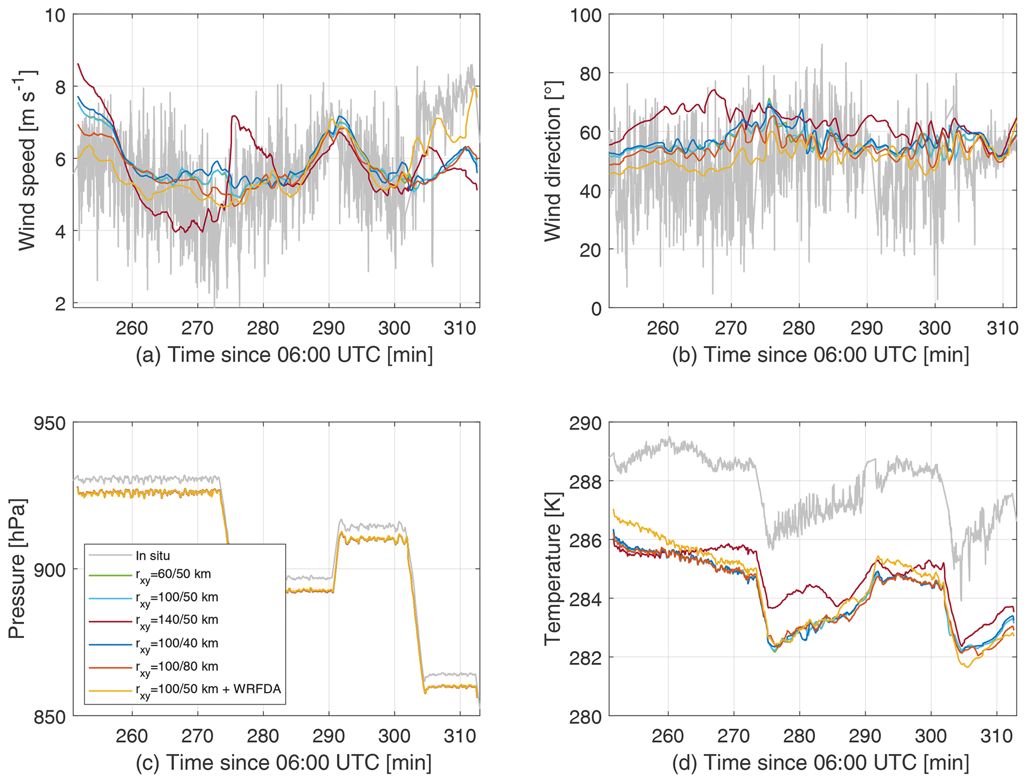
Figure 6 Comparison of 1 Hz wind speed (a), wind direction (b), static pressure (c), and static air temperature (d) as measured aboard the Cessna 208B on 6 June 2018 between 10:00 and 11:20 UTC to ensemble runs with varying r_xy from above. The graphs are plotted as a function of time in minutes since 06:00 UTC.

To verify and validate the observational FDDA approach, non-assimilated meteorological in situ data collected aboard the Cessna 208B are compared to modeled data in Fig. 6. In particular, Fig. 6 compares the 1 Hz wind speed, wind direction, static pressure, and static air temperature as measured on 6 June 2018 between 10:00 and 11:20 UTC with the underwing boom-mounted data acquisition system to ensemble runs with varying r_xy from above. These data were collected approximately 35 km (minimum distance) to 65 km (maximum distance) to the west of the nearest wind lidar during the downwind wall phase of the morning flight (see Fig. 1). Simulated data, extracted at the aircraft positions in space and time, agree with 1 Hz observations of wind speed and direction to within an RMSE of ±0.7 m s⁻¹ (1σ) and ±5^∘ (1σ), respectively. Here, the NCAR Command Language (NCL; Brown et al., 2012) has been used to interpolate from gridded model output to the exact aircraft position in space and time. Modeled wind speed deviates from observed winds during the last 20 min of the downwind wall. A possible reason for this might be that the flight leg was in close vicinity to the PBL top height. A bias of modeled static pressure and static air temperature is evident from the lower panels in Fig. 6. Modeled pressure has a consistent offset of −5 hPa compared to in situ data, and modeled temperature is biased by approximately 2.2 K towards lower values.

4.2 Plume dispersion using FLEXPART-WRF

FLEXPART-WRF version 3.3.2 (Brioude et al., 2013) was used to model the exhaust plumes of known emitters forward in time using the meteorological data (including PBLH) obtained from the WRF simulations described above (see Sect. 4.1) as a driver. The model is set to release 50 000 particles and an arbitrarily chosen total mass of $m_e=\mathrm{1}\times {\mathrm{10}}^{\mathrm{5}}$ kg for each release location during the total simulated time of τ_e= 9 h. The model output is gridded into 100×100 horizontal tiles and 24 vertically stacked layers ranging from ground level up to 3 km in altitude. This results in a horizontal resolution of approximately 1.3 km and a vertical resolution of 50 m near the ground, gradually increasing to 500 m above 2 km in altitude. The domain has been placed inside the nested WRF domain D2 with generous spacing towards the domain boundaries as indicated in Fig. 4 to avoid spurious boundary effects. The main product of the FLEXPART-WRF runs is concentration fields for each release location in units of ng m⁻³, which are scaled a posteriori to deduce the emission rate of each modeled release. Each coal mine ventilation shaft is modeled as a constant, continuous volume source φ_i with a 10 m × 10 m horizontal footprint and extending 10 m in the vertical direction. The volume emitter sizes are based on the construction of typical ventilation shafts in the USCB (Swolkień, 2020).

Mass densities in units of ng m⁻³ can be extracted for the aircraft positions from the model output. The result is an m×n linear forward model matrix K_ji that links scaling factors for emission rates to atmospheric mass density enhancements at the measurement instances, where m is the number of observations available and n is the number of modeled release locations; i.e., K_ji is the mass density that source i contributes to observation j. A scaling coefficient x_i is assigned to each of the n sources ${\mathit{\phi }}_i=m_{e,i}{\mathit{\tau }}_{e,i}^{-\mathrm{1}}$, with the total emission time τ_e,i in seconds and the total mass emitted m_e,i in kilograms for each simulated source. These last two parameters are both assigned in the FLEXPART-WRF input file.

Following a maximum a posteriori (MAP) approach, the scaling coefficients x_i can be found for each of the n modeled sources φ_i and for each of the m observed enhancements y_j making use of a priori information x_a on the emissions of the individual shafts. Following Bayes' theorem the MAP solution is given by the minimum of the cost function (Tarantola, 2004; Jacob, 2007; Rodgers, 2000):

$$\begin{array}{}\text{(1)}& \begin{array}{r}J\left(\mathit{x}\right)={\left(\mathit{x}-{\mathit{x}}_{\text{a}}\right)}^T{\mathbf{S}}_{\text{a}}^{-\mathrm{1}}\left(\mathit{x}-{\mathit{x}}_{\text{a}}\right)\\ +{\left(\mathit{y}-\mathbf{K}\mathit{x}\right)}^T{\mathbf{S}}_{\mathit{ϵ}}^{-\mathrm{1}}\left(\mathit{y}-\mathbf{K}\mathit{x}\right),\end{array}\end{array}$$

with later-defined a priori and observational error covariance matrices S_a and S_ϵ, respectively. The MAP solution can be found by solving for ∇_xJ(x)=0 and is given by

$$\begin{array}{}\text{(2)}& \widehat{\mathbf{x}}={\mathit{x}}_{\text{a}}+\mathbf{G}\left(\mathit{y}-\mathbf{K}\mathit{x}\right),\end{array}$$

with the gain matrix

$$\begin{array}{}\text{(3)}& \mathbf{G}={\mathbf{S}}_a{\mathbf{K}}^T{\left({\mathbf{KS}}_a{\mathbf{K}}^T+{\mathbf{S}}_{\mathit{ϵ}}\right)}^{-\mathrm{1}}.\end{array}$$

By exploiting the averaging kernel A=GK, the number of degrees of freedom for signal d_s can be computed as

$$\begin{array}{}\text{(4)}& d_{\text{s}}=tr\left(\mathbf{A}\right).\end{array}$$

This number describes the reduction in the normalized error in x introduced by the available observations and hence provides a measure for the improvement in knowledge of x, relative to the a priori, due to the observations.

The total emission estimate Φ in units of kg s⁻¹ follows from the scaled sum of the individual contributions φ_i:

$$\begin{array}{}\text{(5)}& \mathrm{\Phi }=\sum _{i=\mathrm{1}}^n{x}_i{\mathit{\phi }}_i.\end{array}$$

Here, the non-negative least squares (NNLS) algorithm (Lawson and Hanson, 1995) has been used to minimize the MAP cost function subject to the constraint x>0. This constraint is equivalent to the absence of negative sources. The NNLS algorithm solves the constrained least squares problem by splitting into active and passive subsets, where active and passive refer to the state of the constraint. The algorithm subsequently solves the unconstrained least squares problem for the passive set.

4.3 Estimating total uncertainty

The outlined approach is based on assumptions, of which the most important ones are a constant emission rate over the timescale of transport from the source to the aircraft; an appropriate atmospheric background vector b (used to compute CH₄ enhancements $\mathit{y}=\mathit{\rho }-\mathit{b}$ from measured mass densities ρ); long lifetime of the species of interest, i.e., no chemical and physical removal on the timescale of a flight; and the model being able to adequately represent the meteorological state variables. To assess uncertainty on the retrieved emission rates, several variables have been selected as most influencing systematic error sources: wind speed, wind direction, PBL height, source dislocation, and an error in sensed mole fractions that is further intended to include an error due to chosen background. Individual contributions of these error sources to total uncertainty can be identified from ensemble model runs with systematically perturbed parameters.

In addition to derived systematic uncertainties, statistical errors related to the MAP fit are to be acknowledged. The statistical uncertainty ϵ_i in the retrieved parameters x_i can be expressed in terms of the parameter covariance matrix $\widehat{\mathbf{S}}$ as

$$\begin{array}{}\text{(6)}& {\mathit{ϵ}}_i=\sqrt{{\widehat{\mathbf{S}}}_{ii}}\end{array}$$

for individual scaling coefficients. For regional estimates we further included off-diagonal elements of $\widehat{\mathbf{S}}$. The parameter covariance matrix $\widehat{\mathbf{S}}$ is computed from the m-by-n dimensional forward model K using

$$\begin{array}{}\text{(7)}& \widehat{\mathbf{S}}={\left({\mathbf{K}}^T{\mathbf{S}}_{\mathit{ϵ}}^{-\mathrm{1}}\mathbf{K}+{\mathbf{S}}_{\text{a}}^{-\mathrm{1}}\right)}^{-\mathrm{1}}.\end{array}$$

Figure 7 (a) Observational covariance augmented with a first-order autoregressive model AR(1) structure with φ=0.7. (b) A priori covariance matrix highlighting correlated clusters from individual ventilation shafts. The scaling factor results from the scaling of the FLEXPART-WRF plume to the designated flux unit kt yr⁻¹.

Due to the different timescales of model output and observations, the observational error covariance matrix S_ϵ cannot simply be taken as a diagonal matrix as this would neglect any correlations. Although the influence on regional estimates is small, these correlations have a significant effect on subregional estimates. The main diagonal of S_ϵ has been estimated from the squared observation uncertainties σ² inflated with a transport model error χ_m obtained from ensemble runs with perturbed parameters (see Sect. 4.6). In order to compensate for tempo-spatio-autocorrelation, we simulated a puff release to check the impulse response of the simulation on a 1 s release from individual sources. We sampled simulated observations from this puff release at the aircraft location in space and time and computed the autocorrelation function (ACF) from a single dispersed puff. The exponential decay of the correlogram suggested to augment the observational covariance matrix with a first-order autoregressive model AR(1) structure with φ=0.7. Figure 7 shows a zoom on the first 400 × 400 elements of this 14 936 × 14 936 matrix to highlight the introduced off-diagonal elements. The measurement uncertainties σ_i were obtained via standard error propagation from the uncertainties associated with different instruments aboard the aircraft needed for the computation of the CH₄ mass density observations (see Eq. 8). Static air temperature, static air pressure, and wind speed can be probed with an uncertainty of σ_T= 0.15 K, σ_p= 1 hPa, and σ_u= 0.3 m s⁻¹ (1s-1σ; Mallaun et al., 2015), respectively. CH₄ mole fractions were sampled with a total uncertainty better than 1.85 ppb (1s-1σ). The main diagonal of the a priori error covariance matrix S_a (i.e., the a priori variances) contains the squared a priori uncertainties, estimated with 50 % of the nominal value. As several shafts cluster around individual mines at distances of not much more than a kilometer, we further introduced a +0.5 correlation into the mines belonging to the same cluster and mining company and added local information (see review comment by Jaroslaw Necki, https://doi.org/10.5194/acp-2020-962-SC1). The final a priori error covariance matrix is depicted in Fig. 7. The scaling factor results from the scaling of the FLEXPART-WRF plume to the designated flux unit kt yr⁻¹.

4.4 Case study – 6 June 2018

Figure 8 shows a time series of the measured and modeled CH₄ mass density enhancement as a function of flight time during the downwind wall phase with the atmospheric background subtracted and source coefficients x_i already optimized (according to Eq. 1).

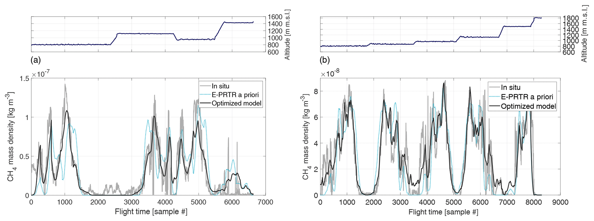
Figure 8 Time series of the in situ measured (gray) and modeled CH₄ mass density (solid black) with subtracted background as a function of flight time during the downwind wall phase of the morning (a) and afternoon (b) flight on 6 June 2018 with optimized source coefficients x_i. The dotted light blue line corresponds to the same forward simulation using scaling coefficients deduced from E-PRTR 2017.

Figure 9 (a) Interpolated cross section of the model output along the downwind wall including scattered in situ observations of CH₄ for the morning flight on 6 June 2018. The color bar also applies to the isolines on the right. (b) Top-down view of the model output and the downwind wall observations ρ at 750 $\mathrm{m}\mathrm{a}.\mathrm{g}.\mathrm{l}.$ with underlaid topography. Triangles mark simulated emitters with colors corresponding to the optimized source strengths. Gray isolines correspond to non-fuel-exploitation emissions. Both panels show a snapshot of the model output at one fixed time chosen as the center time of the downwind wall phase.

The measured scalar mass density ρ has been deduced from the ideal gas law pV =mR_sT (mass m, specific gas constant $R_s=R/M$, and molar mass of CH₄ M) using the in situ measured static air temperature and static air pressure according to

$$\begin{array}{}\text{(8)}& {\mathit{\rho }}_x={\displaystyle \frac{m_x}{V_{\text{air}}}}={\displaystyle \frac{m_x}{m_{\text{air}}}}{\left({\displaystyle \frac{p}{RT}}\right)}_{\text{air}},\end{array}$$

where m_x denotes the total mass of the species of interest. The unitless coefficient $m_x{m}_{\text{air}}^{-\mathrm{1}}=c_x{M}_x{M}_{\text{air}}^{-\mathrm{1}}$ is obtained from the sensed CH₄ mole fractions c_x in units of mol mol⁻¹.

Prior to conversion, the atmospheric background has to be subtracted from the observed c_x. The choice of background is to some extent ambiguous because there is no clear edge between background and in-plume sampling. This contributes to total flux estimation uncertainty, as will be discussed later. Here, a piecewise linear interpolation between the outermost boundaries of each of the four flight legs (see Fig. 9) has been considered the best guess of atmospheric background. The mean value of 20 samples has been used on both edges of each flight leg. Using this approach, latitudinal and longitudinal gradients in background CH₄ mole fractions are accounted for by using both edges of each flight leg. Vertical gradients in background CH₄ levels are accounted for by treating each constant-altitude flight leg separately.

From Fig. 8 a good overall match between model (solid black line) and in situ observations (gray) is apparent with a mean bias of $\mathrm{2.5}\times {\mathrm{10}}^{-\mathrm{9}}$ kg m⁻³ and a root mean square error of $\mathrm{1.6}\times {\mathrm{10}}^{-\mathrm{8}}$ kg m⁻³. Some of the minor structure is not reproduced in detail by the model, which is to be expected due to the model's 3 km horizontal grid resolution. The reason for the discrepancy between model and the first few hundred observations in Fig. 8 becomes more obvious when looking at the 2D scene shown in Fig. 9. The left panel of Fig. 9 shows a cross section of the model output along the downwind wall including the in situ observations of ρ. The right panel of Fig. 9 depicts the top-down view of the model output and the downwind wall observations at a fixed altitude of 750 $\mathrm{m}\mathrm{a}.\mathrm{g}.\mathrm{l}$. It should be noted here that both panels show a snapshot of the model output at one fixed time chosen as the center time of the downwind wall.

The discrepancy between model and observation at the lowermost (first in time) flight leg, corresponding to the southernmost trajectory section in Fig. 9 (right panel), cannot be reproduced by any of the included emission sources. A possible source is urban CH₄ emissions of Krakow, located to the east of the USCB region. An area source, covering the greater city area, has therefore been included in the model. Its influence can be seen at the rightmost edge of Fig. 9 (right panel). Although we identified the city of Krakow as a possible source, we omitted it in the USCB emission estimates, as it does not officially belong to the USCB area. There are other parts in the time series where the model either underestimates (e.g., times around observation numbers 2000–3000 and 4000–4500) or overestimates (e.g., around observation number 6000) emissions. This might well be related to sources not taken into account or deficiencies in wind speed, wind direction, PBL height, etc.

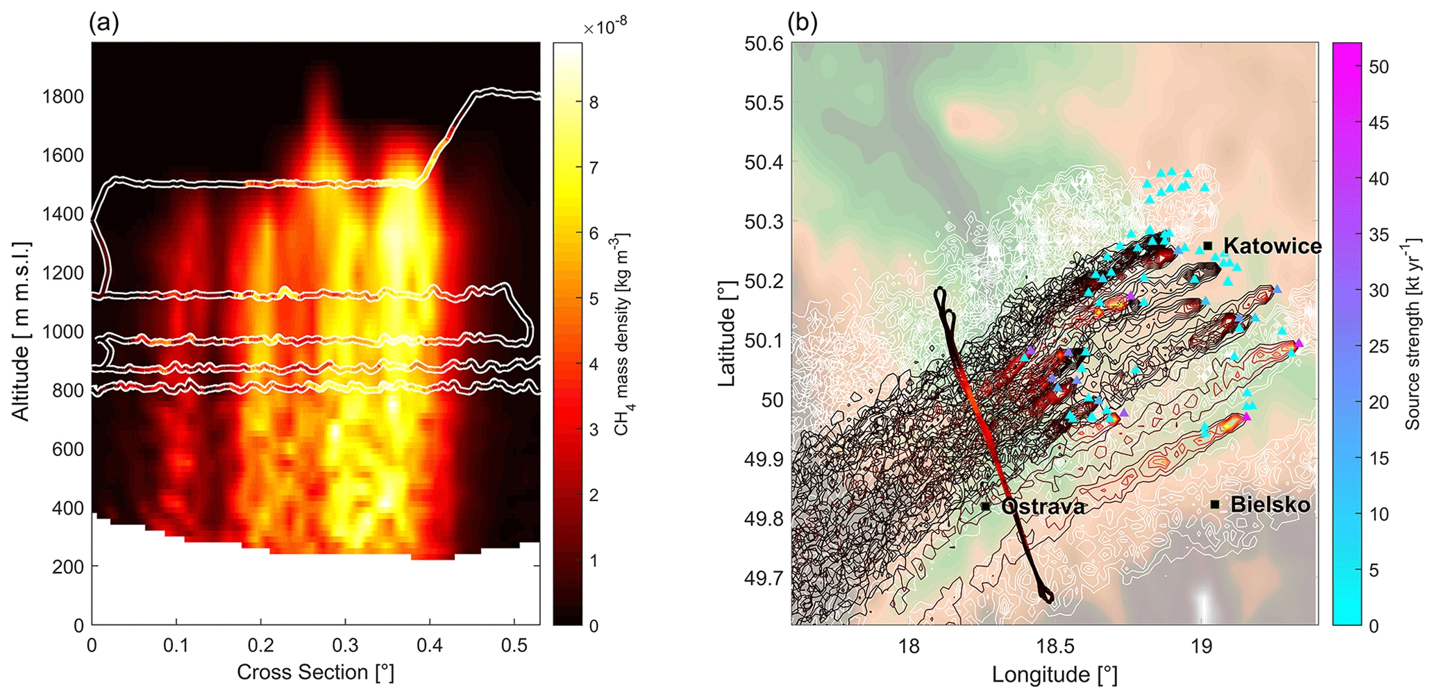
Figure 10 (a) Interpolated cross section of the model output along the downwind wall including scattered in situ observations of CH₄ for the afternoon flight on 6 June 2018. The color bar also applies to the isolines on the right. (b) Top-down view of the model output and the downwind wall observations ρ at 750 $\mathrm{m}\mathrm{a}.\mathrm{g}.\mathrm{l}.$ with underlaid topography. Gray isolines correspond to non-fuel-exploitation emissions. Triangles mark simulated emitters with colors corresponding to the optimized source strengths. Both panels show a snapshot of the model output at one fixed time chosen as the center time of the downwind wall phase.

The instantaneous fuel-exploitation emission estimate directly follows from the optimized parameters x_i via Eq. (5). The emission estimate obtained for the morning flight on 6 June 2018 using the model-based approach amounts to Φ= 451 ± 77 kt yr⁻¹. It differs from the yearly averaged inventorial emission estimates for the USCB region by approximately −28 % for EDGAR v4.3.2 and +1 % for the E-PRTR inventory (excluding simulated non-fuel-exploitation sources). In addition to the coal mine emissions, approximately 27 kt yr⁻¹ of CH₄ are estimated to emanate from simulated non-coal-mine sources. The retrieval for the morning flight yields 48 degrees of freedom for signal and a total of 35 out of 74 modeled sources actively emitting. Here, the large number of degrees of freedom for signal is indicative of the validity of the total emission estimate. The latter can be confirmed by the negligible impact of the a priori $\sum \left(\mathbf{1}-\mathbf{A}\right){\mathit{x}}_{\text{a}}$ versus the observations ∑Ax in the emission estimate. The algorithm makes use of the large number of modeled sources to enable a total emission estimate plus additional information on individual sources.

To enhance confidence in the emission estimate, an afternoon flight of the DLR Cessna 208B was carried out a few hours after the morning flight ended on 6 June 2018. Due to consistent wind directions on that day, the flight pattern was kept as close as possible to the morning flight. The flight trajectories for both flights are depicted in Fig. 1. The right panel in Fig. 8 shows the corresponding time series of the measured and modeled CH₄ mass density as a function of flight time during the downwind wall phase with source coefficients x_i already optimized. Like for the morning flight a good overall match between model and in situ observations can be observed with a mean bias of $\mathrm{3}\times {\mathrm{10}}^{-\mathrm{10}}$ kg m⁻³ and a root mean square error of $\mathrm{1}\times {\mathrm{10}}^{-\mathrm{8}}$ kg m⁻³. The sensed mixing ratios are lower compared to the morning flight due to a further developed and hence more diluted boundary layer in the afternoon. The corresponding snapshot 2D scene is depicted in Fig. 10, with the left panel showing a cross section of the model output along the downwind wall including the in situ observations of ρ. The right panel of Fig. 10 shows the top-down view and the downwind wall observations as before. Both panels show a snapshot of the model output at the center time of the downwind wall phase. It is evident from Fig. 10 that the inclined boundary layer height observed during the flight is nicely captured by the model. Boundary layer depth is generally enhanced compared to the morning flight. Plume trajectories are streamlined implying consistent winds over time.

The fuel-exploitation emission estimate obtained for the afternoon flight on 6 June 2018 using the model-based approach amounts to Φ= 423 ± 79 kt yr⁻¹. The obtained instantaneous emission estimate differs from the yearly averaged inventorial emission values for the USCB region by approximately −32 % for EDGAR v4.3.2 and −6 % for the E-PRTR inventory (excluding simulated non-fuel-exploitation sources). The retrieval for the afternoon flight yields 31 kt yr⁻¹ of CH₄ from simulated non-coal-mine sources, 42 degrees of freedom for the signal, and a total of 38 out of 74 simulated coal mine sources actively emitting. Both flights yield similar d_s values, indicating that not all information stems from observations alone. Hence, neither flight can be used alone to retrieve all modeled sources. In an effort to minimize the dependency on the a priori, both flights will be analyzed together in the next section.

4.5 Subregional emission estimates

The model-based approach provides a unique advantage over established mass balance techniques in terms of spatial information, as it enables attributing sensed CH₄ mole fractions to remote sources at distances of tens to hundreds of kilometers. The achievable level of confidence for these subregional estimates however strongly depends on the observational data. The total emission estimate has been introduced in Sect. 4.2 as the sum over n sources φ_i that are individually scaled with a coefficient x_i. The emission rate Φ_i corresponding to the ith source is thus given by x_iφ_i. By including all n sources in the state vector, individual scaling coefficients can be derived for individual sources. Here, the availability of data from two research flights on 6 June 2018 was exploited to estimate subregional emission rates Φ_i for individual sources. As the mean wind direction differed by ≤ 10 % between the two flights, uncertainty on the shaft level remained large and observational data are too limited for a more specific estimate. With mission planning further optimized for the Bayesian inversion from airborne in situ data, as presented in this paper, these uncertainties can potentially be narrowed down in future campaigns. The retrieval yields d_s=32 with 53 sources actively emitting.

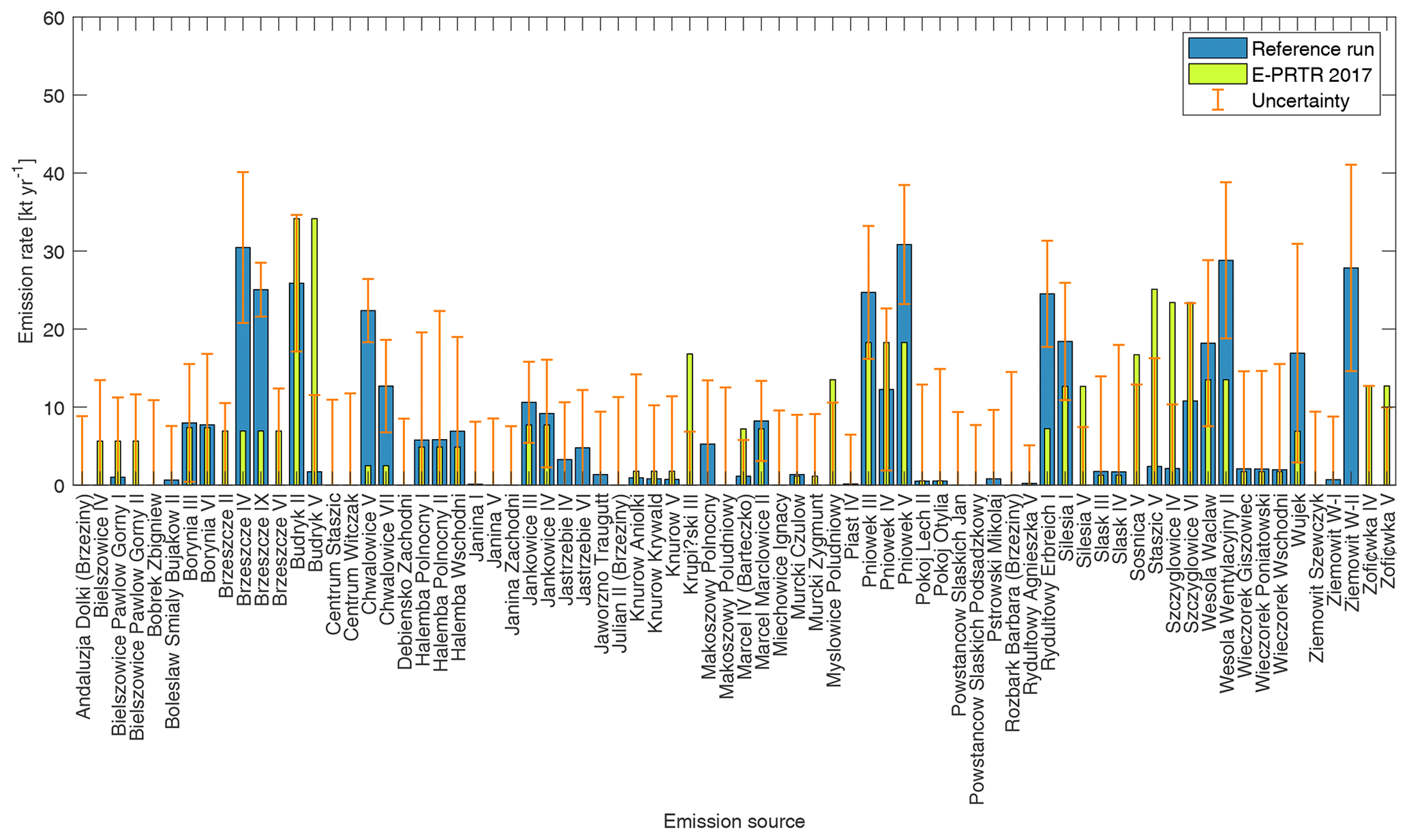
Figure 11 Emission estimates Φ_i (blue bars) in kt yr⁻¹ for 74 individual mining shafts using the morning and afternoon flight of 6 June 2018. Slim green bars are the reported yearly average values for each mining company (E-PRTR 2017) evenly distributed among the respective ventilation shafts. The orange error bars stem from the quadrature sum of the statistical uncertainties ϵ_i (computed from the parameter covariance matrix $\widehat{\mathbf{S}}$) and the uncertainties σ_ensemble derived from a variational ensemble with systematically perturbed parameters.

Figure 11 illustrates Φ_i in kt yr⁻¹ for all modeled mining shafts, taking into account both research flights on 6 June 2018. The blue bars represent the estimated Φ_i and are to be related to the yearly average values (slim green bars) for each mining company reporting to E-PRTR 2017 for illustrative purposes. The estimated uncertainty depicted in Fig. 11 includes systematic uncertainties derived from a variational ensemble and statistical uncertainties due to the fit algorithm used (see Sect. 4.3). The variational ensemble introduced in Sect. 4.3 includes scaling coefficients x_i subject to systematic variations in key sources of uncertainty. Systematic uncertainties for each source are directly obtained from this ensemble run. Differences in estimated and reported (E-PRTR 2017) Φ_i values are evident. This is however to be expected due to the comparison of instantaneous emission estimates and yearly averages. Figure 12 shows the a posteriori correlation matrix as deduced from the MAP covariance matrix. The matrix indicates that there remained some uncertainty regarding to which shaft the emissions had to be assigned.

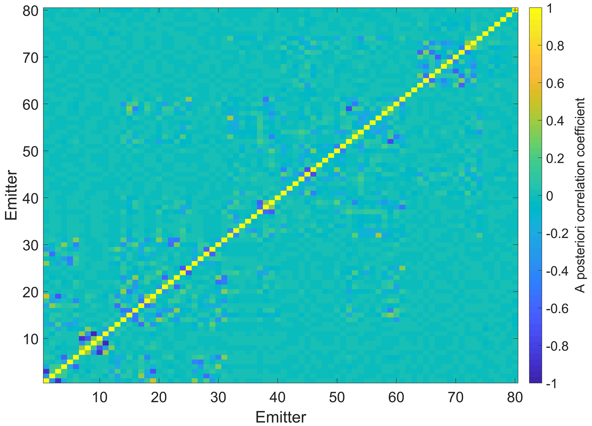
Figure 12 A posteriori correlation matrix as deduced from the a posteriori covariance matrix showing there remained some uncertainty regarding to which shaft the emissions had to be assigned.

4.6 Uncertainty analysis

The influence of several variables on the total flux estimate Φ has been computed from eight sensitivity runs with symmetrically perturbed parameters. The systematic transport model uncertainty is subsequently estimated as the standard deviation of this ensemble. Figure 13 shows the influence of an error in wind speed (σ_u= 0.9 m s⁻¹), wind direction (σ_d= 5 ^∘), PBL height (σ_pbl= 100 m), and a source dislocation (σ_sd= 1 km) on total uncertainty for the flights detailed in the previous section. An assumed error in sensed mole fractions (σ_c= 10 ppb) is intended to include an error due to wrongly chosen background. The error in wind speed σ_u is taken as the standard deviation of the difference between WRF modeled wind and non-assimilated in situ observations from the data depicted in Fig. 6.

Figure 13 Ensemble runs to assess uncertainty in the flux estimates derived using a model-based approach. All selected error sources contribute to total uncertainty on a similar level.

The same holds for the wind direction. The difference between modeled data and observations should therefore reflect overall uncertainty in these variables. Two spiral-up soundings out of the PBL revealed a boundary layer height of 1150 m at 09:37 UTC and 1300 m at 11:45 UTC. Based on these two soundings, the uncertainty in boundary layer depth is estimated with σ_pbl= 100 m for the downwind wall phase between 10:00 and 11:00 UTC. For this sensitivity analysis, the WRF fields were perturbed systematically during the FLEXPART read phase in readwind.f90. The source dislocation was implemented in the FLEXPART configuration file. It is evident from Fig. 13 that all selected error sources contribute on a similar level to total systematic uncertainty, which is ultimately computed as the standard deviation of the ensemble.

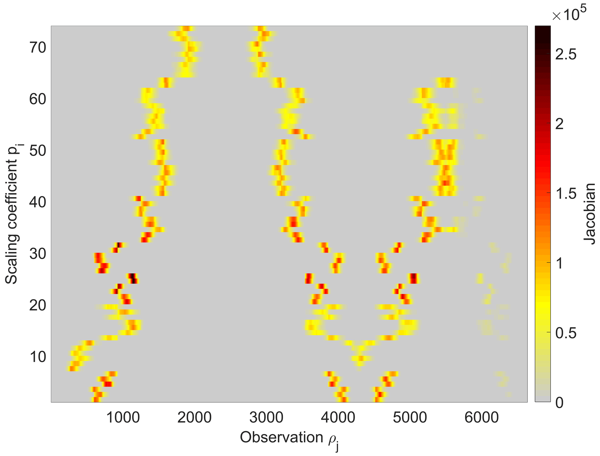
Figure 14 Jacobian with respect to x_i and the observations y_j for the morning flight on 6 June 2018. All scaling coefficients x_i are sensitive to variations in y_j and can therefore be deduced from a MAP fit. Measurements centered around observation 2300 are not covered by the model and are thus obsolete for flux estimation using this particular flight.

In addition to the derived systematic uncertainties, statistical errors related to the MAP fit have been computed following Sect. 4.3. Figure 14 depicts the Jacobian K with respect to x_i and the observations of the morning flight on 6 June 2018. It describes the change in residuals introduced by a change in parameter x_i. From this figure, it can be seen that all 74 modeled coal mine sources were sampled by the aircraft using the chosen flight pattern, as all scaling coefficients are represented in the Jacobian. For the fluxes emanating from the USCB area, the statistical uncertainty ϵ_i computed from the Jacobian following Eqs. (6) and (7) amounts to approximately 66 kt yr⁻¹ or 15 %, respectively.

Ultimately, the total uncertainty for the morning flight (same for the afternoon flight) on 6 June 2018 is the quadrature sum of systematic (44 kt yr⁻¹) errors from the ensemble runs and statistical uncertainty (66 kt yr⁻¹) from the fitting algorithm adding up to approx. 17 % relative uncertainty.

5 Conclusions

A modified Aerodyne dual QCLS instrument was deployed aboard the DLR Cessna 208B in the context of the CoMet 1.0 campaign in early summer 2018 with the goal of estimating hard-coal-mine CH₄ emissions emanating from the USCB area – Europe's largest coal extraction region. Intensive mining activities and the heavy industry spread around the city of Katowice lead to significant amounts of GHGs emitted into the atmosphere. The reported inventorial CH₄ emission rates for the entire USCB region amount to 720 kt yr⁻¹ (EDGAR v4.3.2) and 448 kt yr⁻¹ (E-PRTR 2017). The latter corresponds to 12.5 $\mathrm{Mt}{\mathrm{CO}}_{\mathrm{2}}\mathrm{eq}.{\mathrm{yr}}^{-\mathrm{1}}$ using a value of CH₄ GWP₁₀₀=28 from the IPCC Fifth Assessment Report (Pachauri et al., 2014). Assuming an average carbon content of 75 %, a net calorific value of 29 MJ kg⁻¹, an emission factor of 94 t CO₂ (TJ)⁻¹, and the approximate 75×10⁶ t of coal extracted from the USCB every year results in yearly CO₂ emissions of 205 Mt CO₂ yr⁻¹ from burning of the extracted coal. The CH₄ emissions from mining alone therefore make up approximately 6 % in terms of GWP.

Estimates of coal mine CH₄ emissions in the USCB were derived using a model approach based on the Eulerian WRF model and the Lagrangian particle dispersion model FLEXPART-WRF. Data assimilation further exploits the availability of additional data products, e.g., wind lidar soundings during the CoMet 1.0 campaign. Due to the known locations of the coal mine ventilation shafts, sources are modeled forward in time assuming a constant emission rate. Modeled data are then extracted at the aircraft positions in space and time and compared to actual airborne in situ observations. Here, meteorological driver data were generated using the WRF v4.0 model with continuous assimilated wind lidar soundings using WRF's OBS-FDDA and WRFDA subsystems. After validation with unassimilated in situ measurements, data were fed into the Lagrangian particle dispersion model FLEXPART-WRF and used to model the exhaust plumes of the ventilation shafts. Using an inverse modeling approach, a priori emission data from E-PRTR 2017 are optimized to allow a better fit to the observations. Thereby, total emission estimates for the USCB area of Φ= 451 ± 77 kt yr⁻¹ and Φ= 423 ± 79 kt yr⁻¹ were obtained for a morning flight and an afternoon flight on 6 June 2018, respectively. This includes non-fuel-exploitation fluxes, estimated with 27 and 31 kt yr⁻¹ for the morning and afternoon flights, respectively. Morning and afternoon flights differ by less than 4 % corresponding to an excellent agreement well within the uncertainty range. The obtained emission estimate differs from the inventorial emission estimates by approximately −28 %/−32 % for the EDGAR v4.3.2 inventory (morning flight/afternoon flight) and +1 %/−6 % for the E-PRTR inventory (excluding non-fuel-exploitation sources), respectively. Differences in estimated and reported emission rates are however expected due to the comparison of instantaneous estimates and yearly averages. This is in line with previous studies hinting at EDGAR v4.3.2 overestimating CH₄ emissions in the USCB (Luther et al., 2019; Fiehn et al., 2020). Uncertainty estimates include systematic contributions from ensemble runs and statistical uncertainty introduced by the fitting algorithm. Data from both research flights are further exploited to estimate individual source contributions. Differences between individual estimates and E-PRTR reported emissions are observed. This is expected due to several reasons: a limited number of measurements relative to the yearly averages provided in the inventories, wind directions do not differ by much between the two flights, and the evenly distributed emissions among the ventilation shafts for each mining company. In general, the approach described herein delivers more information compared to the conventional mass balance, albeit at increased effort: wind lidars need to be deployed during the measurement campaign, models need to be run, wind lidar data need to be assimilated, and inverse estimation techniques need to be applied. The additional possibility of remote source attribution, however, coupled with the results obtained in Sect. 4.2 for the regional USCB anthropogenic CH₄ emissions makes this approach a potent alternative to the mass balance technique. Although retrieving estimates for individual emitters is not possible using only single flights, due to sparse data availability, the combination of two or more flights allows for exploiting different meteorological conditions to enhance confidence in facility-level estimates.