Responses of Arctic black carbon and surface temperature to multi-region emission reductions: a Hemispheric Transport of Air Pollution Phase 2 (HTAP2) ensemble modeling study

Black carbon (BC) emissions play an important role in regional climate change in the Arctic. It is necessary to pay attention to the impact of long-range transport from regions outside the Arctic as BC emissions from local sources in the Arctic were relatively small. The task force Hemispheric Transport of Air Pollution Phase 2 (HTAP2) set up a series of simulation scenarios to investigate the response of BC in a given region to different source regions. This study investigated the responses of Arctic BC concentrations and surface temperature to 20 % anthropogenic emission reductions from six regions in 2010 within the framework of HTAP2 based on ensemble modeling results. Emission reductions from East Asia (EAS) had the most (monthly contributions: 0.2–1.5 ng m⁻³) significant impact on the Arctic near-surface BC concentrations, while the monthly contributions from Europe (EUR), Middle East (MDE), North America (NAM), Russia–Belarus–Ukraine (RBU), and South Asia (SAS) were 0.2–1.0, 0.001–0.01, 0.1–0.3, 0.1–0.7, and 0.0–0.2 ng m⁻³, respectively. The responses of the vertical profiles of the Arctic BC to the six regions were found to be different due to multiple transport pathways. Emission reductions from NAM, RBU, EUR, and EAS mainly influenced the BC concentrations in the low troposphere of the Arctic, while most of the BC in the upper troposphere of the Arctic derived from SAS. The response of the Arctic BC to emission reductions in six source regions became less significant with the increase in the latitude. The benefit of BC emission reductions in terms of slowing down surface warming in the Arctic was evaluated by using absolute regional temperature change potential (ARTP). Compared to the response of global temperature to BC emission reductions, the response of Arctic temperature was substantially more sensitive, highlighting the need for curbing global BC emissions.

1 Introduction

Black carbon (BC) is one of the short-lived climate forcers (SLCFs; AMAP, 2015) and was regarded as the second-largest contributor to global warming, only inferior to carbon dioxide (Bond et al., 2013). BC over the Arctic can perturb the radiation balance in a number of ways. Direct aerosol forcing occurred through absorption or scattering of solar (shortwave) radiation. BC is the most efficient atmospheric particulate species at absorbing visible light (Bond et al., 2013); the added atmospheric heating will subsequently increase the downward longwave radiation to the surface and warm the surface (AMAP, 2011). Radiative forcing by BC can also result from aerosol–cloud interactions that affected cloud microphysical properties, albedo, extent, lifetime, and longwave emissivity (Twomey, 1977; Garrett and Zhao, 2006). BC has an additional forcing mechanism after depositing onto snow and ice surfaces (Clarke and Noone, 1985). The surface albedo of snow and ice could be reduced and further enhanced the absorption of solar radiation at the surface. In the Arctic, surface temperature responses were strongly linked to surface radiative forcing as the stable atmosphere of the region prevented rapid heat exchange with the upper troposphere (Hansen and Nazarenko, 2004).

The Arctic has been warming twice as rapidly as the world in the past 50 years and has experienced significant changes in its ice and snow covers as well as permafrost (AMAP, 2017). Reductions in carbon dioxide emissions are the backbone of any meaningful effort to mitigate climate forcing. But even if significant reductions in carbon dioxide are made, slowdown of the temperature rise in the Arctic and the sea level rise caused by the melting of glaciers may not be achieved in time. Hence, the goal of slowing down the deterioration of the Arctic may best be achieved by also targeting shorter-lived climate forcing agents, especially those that could impose appreciable surface forcing and trigger regional-scale climate feedbacks pertaining to the melting of sea ice and snow. Modeling studies by UNEP/WMO (2011) and Stohl et al. (2015) suggested that the climate response of SLCF mitigation was strongest in the Arctic region. AMAP (2011 and 2015) as well as Sand et al. (2016) demonstrated that the northern areas in the Arctic had the largest temperature response per unit of emission reductions in SLCFs, with the Nordic countries (Denmark, Finland, Iceland, Norway, and Sweden) and Russia having the largest impact compared to other Arctic countries such as the United States and Canada.

The few studies that investigated specific regional aerosol forcing (Shindell and Faluvegi, 2009; Shindell et al., 2012; Teng et al., 2012) typically used a single climate model at a time to investigate the climate response to idealized, historical, or projected forcing. However, different models varied considerably in the representation of aerosols and radiative properties, resulting in large uncertainties in simulating the aerosol radiative forcing (Myhre et al., 2013; Shindell et al., 2013). When investigating the climate response to regional emissions, such uncertainties were likely to be confounded even further by the variability between models in regional climate and circulation patterns and variation in the global and regional climate sensitivity (the amount of simulated warming per unit radiative forcing). Hence, the task force Hemispheric Transport of Air Pollution Phase 2 (HTAP2; http://www.htap.org/, last access: 3 June 2021), incorporating multiple global models, can avoid the great uncertainty in a single model to a certain degree, with the aim of improving model estimates of the impacts of intercontinental transport of air pollutants on climate, ecosystems, and human health (Galmarini et al., 2017). To date, the HTAP2 results have been explored from a variety of scientific and policy-relevant perspectives. For instance, by comparing against observations, sulfur and nitrogen depositions during HTAP2 had been significantly improved compared to HTAP1. From 2001 to 2010, the global nitrogen deposition increased 7 %, while the global sulfur deposition decreased 3 % (Tan et al., 2018a). The significant impacts of hemispheric transport on the deposition were specifically focused, and the deposition over the coastal regions was more sensitive to hemispheric transport than the non-coastal continental regions (Tan et al., 2018b). Jonson et al. (2018) assessed the contributions from different world regions to European ozone levels, and contributions from the non-European regions were mostly from the North America and eastern Asia, larger than those from European emissions. Hogrefe et al. (2018) found that the simulated ozone over the continental US varied very differently by digesting boundary conditions from four hemispheric or global models. The impact of emission changes from six major source regions on global aerosol direct radiative forcing was estimated (Stjern et al., 2016). In the local source regions, the radiative forcing associated with SO${}_{\mathrm{4}}^{\mathrm{2}-}$ was strengthened (25 %), while that from BC was weakened (37 %) due to a 20 % emission reduction. Liang et al. (2018) estimated that global air-pollution-related premature mortality from exposure to PM_2.5 and ozone and the interregional transport lead to more deaths through changes in PM_2.5 than in O₃. However, the source region contributions to Arctic BC and the spread among multi-model results have been rarely explored from the perspective of the HTAP2 initiative.

This study aims to investigate the responses of Arctic BC concentrations and surface temperature to 20 % anthropogenic emission reductions from different regions in the Northern Hemisphere (NH). A comparison of six global modeling works within the framework of HTAP2 experiments for the Arctic region in 2010 was presented. The ensemble modeling results were used to apportion the contribution from different source regions to the near-surface and vertical black carbon in the Arctic. In addition, the Arctic surface temperature responses to the emission reductions were estimated.

2 Methodology

2.1 HTAP2 experiments

HTAP2 developed a harmonized emissions database covering all countries and the major sectors for global and regional modeling from 2008 to 2010. The emissions database was obtained from the nationally reported emissions (e.g., National Emission Inventory for the United States), the regional scientific inventories (e.g., the European Monitoring and Evaluation Programme (EMEP) and the Netherlands Organisation for Applied Scientific Research (TNO) for Europe and the Model Inter-Comparison Study for Asia (MICS–Asia III)), and the Emissions Database for Global Atmospheric Research data (EDGARv4.3) for the rest of the world (mainly South America, Africa, Russia, and Oceania). Biomass burning emissions were not prescribed in HTAP2. Temporal resolution of data sources was monthly, and thus the HTAP2 emission inventory provided harmonized emission data with monthly resolution for all the air pollutants including BC. It should be noted that the emissions of international shipping and international aviation in HTAP2 were considered constant over the year. It was recommended that modeling groups use the Global Fire Emissions Database (GFED4; http://globalfiredata.org/, last access: 3 June 2021) with a temporal resolution of daily or 3 h intervals. The detailed information of different regional inventories can be found in Janssens-Maenhout et al. (2015).

Emission perturbations were conducted in sensitivity simulations to investigate the response of various air pollutants in a given region to different source regions. In this study, the Arctic region was the targeted receptor region of interest. Six source regions in HTAP2 experiments, namely East Asia (EAS), Europe (EUR), Middle East (MDE), North America (NAM), Russia–Belarus–Ukraine (RBU), and South Asia (SAS), were selected to demonstrate their influences on the BC concentrations over the Arctic region (Fig. 1a). Two emission scenarios were designed for the HTAP2 simulation to explore the source–receptor relationships, i.e., the base scenario (BASE) with no emission reduction and the control scenario (EASALL, EURALL, MDEALL, NAMALL, RBUALL, and SASALL) with 20 % reduction in all anthropogenic emissions in six regions, respectively.

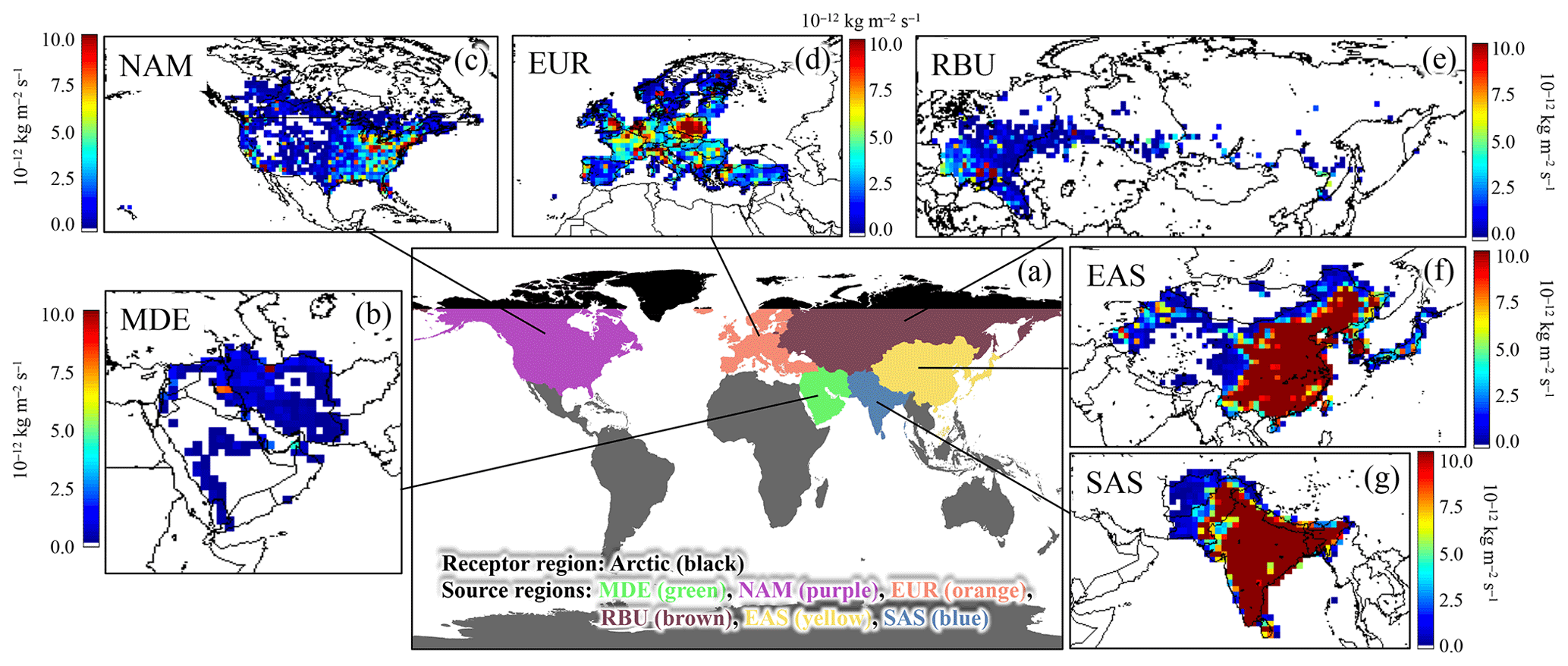
Figure 1 (a) The sketch map of receptor and source regions. (b–g) Spatial distributions of 20 % reduction in annual BC emission in the six source regions in 2010. MDE: Middle East; EUR: Europe; RBU: Russia–Belarus–Ukraine; NAM: North America; EAS: East Asia; SAS: South Asia. The unit legends from (b) to (g) are the same (10⁻¹² kg m⁻² s⁻¹).

2.1.1 Anthropogenic emission reductions in BC in HTAP2

Anthropogenic BC emission sectors included power plants, industries, transportation, shipping, aviation, agriculture, and residential sectors. The emission inventory had a monthly temporal resolution and a spatial resolution of 0.1^∘ × 0.1^∘. The total anthropogenic emissions and 20 % emission reductions in BC in six source regions of HTAP2 in 2010 are presented in Table 1. The higher BC emission reductions were found in the EAS and SAS with values of 355.6 and 232.5 Gg yr⁻¹, respectively, while they were much lower in the MDE and RBU, with values of 5.3 and 18.6 Gg yr⁻¹, respectively. The BC emission reductions in the EAS, EUR, and RBU showed significant monthly variations, with higher values from November to March, while the monthly variations were not obvious in the MDE, NAM, and SAS.

Table 1 Total anthropogenic emissions and 20 % emission reductions in BC in different regions of HTAP2 in 2010 (unit: Gg yr⁻¹).

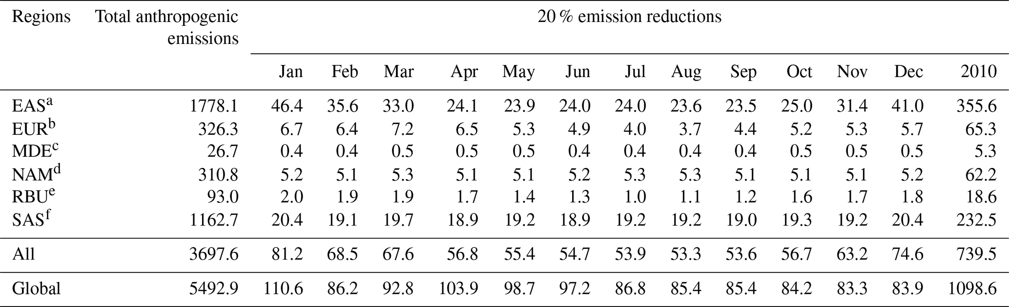
^a East Asia. ^b Europe. ^c Middle East. ^d North America. ^e Russia–Belarus–Ukraine. ^f South Asia.

Figure 1b–g illustrate the spatial distribution of the 20 % reductions in annual BC emissions in six source regions in 2010. It can be found that the most intense reductions in BC emissions in EAS and SAS were concentrated in East China and India, respectively, which were mainly attributed to emissions from residential sectors, followed by transportation and industries. The BC emission reductions in EUR were widely distributed, with high values in central Europe and residential and transportation sectors accounting for the largest proportion. The reductions near the Arctic circle could be found in the north of EUR, NAM, and RBU. For MDE, most BC was emitted from Iran, which is located in the northeast of this region. Overall, the spatial pattern of BC emission reductions in six regions was closely related to the spatial distribution of the human population.

2.1.2 Model description

Considering that the simulations should cover all months of 2010 and all emission source regions, five global models (i.e., CAMchem, CHASER_re1, GEOS-Chem, GOCART–v5, and Oslo CTM3–v2) were incorporated to simulate the responses of BC concentrations in the Arctic to 20 % BC emission reductions from EAS, EUR, MDE, NAM, RBU, and SAS, respectively. The brief information of model configurations is listed in Table 2. As required by HTAP2, all simulations should include a spin-up time of 6 months prior to the period of interest. The outputs from all models are available upon request from http://aerocom.met.no (last access: 3 June 2021). The time resolution of the outputs used in this study is monthly for all models, although models were run at a finer resolution (e.g., daily or hourly). The model outputs for air pollutants were originally provided in the unit of mass mixing ratio (MMR; kg kg⁻¹). To facilitate comparison between model and observation and further data analysis, we converted the original units into ng m⁻³ based on the ideal gas law (Aamaas et al., 2017).

Table 2 Configurations of models used in this study.

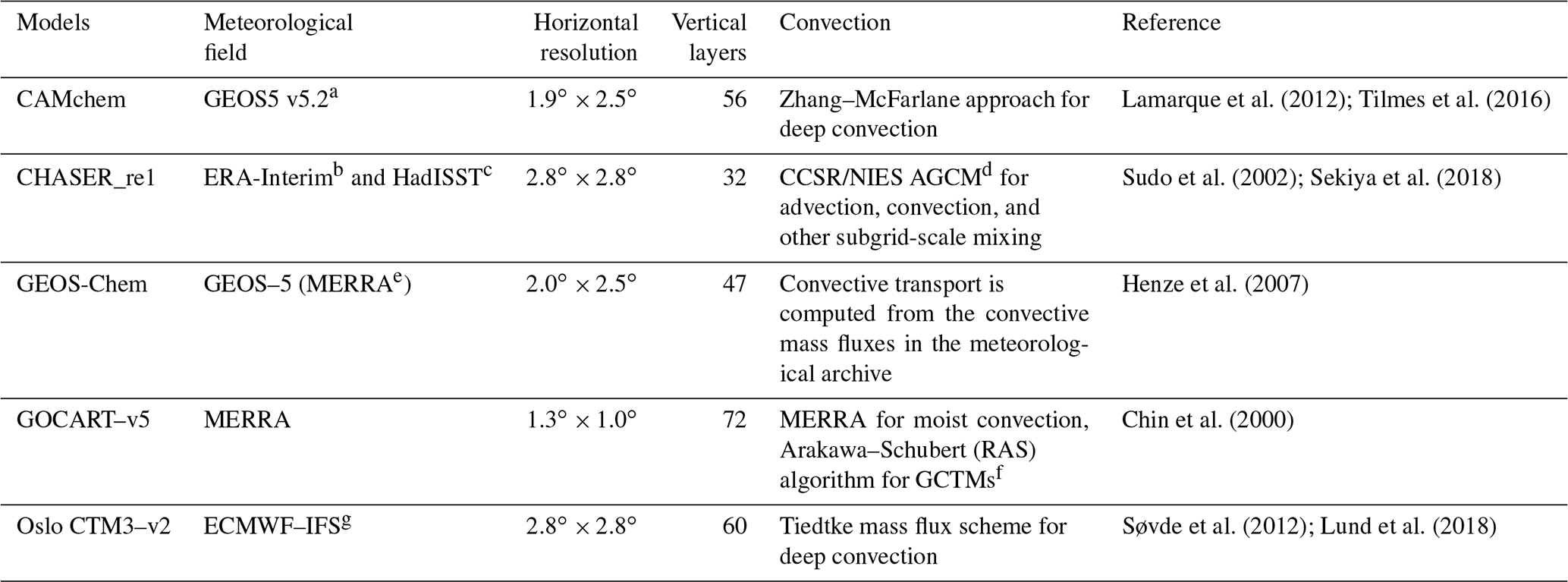
^a Goddard Earth Observing System, Version 5. ^b Interim European Centre for Medium-Range Weather Forecasts (ECMWF) Re-Analysis data. ^c Hadley Centre sea ice and sea surface temperature (SST) data set. ^d Center for Climate System Research/National Institute for Environment Studies (CCSR/NIES) atmospheric general circulation model (AGCM). ^e Modern Era Retrospective-Analysis for Research and Applications. ^f Global chemical transport models. ^g ECMWF's Integrated Forecast System (IFS) model.

2.2 Calculation of the temperature response to BC emission reduction

The climate effects of air pollutants have been the focus of climate change research since the last century (IPCC, 1990, 2001). In the last few years, the metrics for estimating this kind of effect have been constantly improving (Shindell et al., 2012; Bond et al., 2013; Smith and Mizrahi, 2013; Stohl et al., 2015). The Intergovernmental Panel on Climate Change (IPCC) used the global warming potential (GWP) as a method for comparing the potential climate impact of emissions of different greenhouse gases (IPCC, 1990). GWP is the time-integrated radiative forcing due to a pulse emission of a given species over some given time horizon (commonly 20, 100, or 500 years) relative to a pulse emission of carbon dioxide. GWP does not purport to represent the impact of air pollutant emissions on temperature. Although a short-lived climate pollutant (SLCP) could have the same GWP as a long-lived climate pollutant, identical (in mass terms) pulse emissions could cause a different temperature change at a given time because long-lived climate pollutants accumulate in the climate system, while short-lived climate pollutants can be broken down by various processes. Consequently, warming caused by long-lived climate pollutants is determined by total cumulative emissions to date, while the warming due to short-lived climate pollutants is determined more by the current rate of emissions in any given decade and depends much less on historical emissions. This means the importance of SLCP emissions is often overstated based on GWP. Shine et al. (2005) proposed the global temperature change potential (GTP) as a replacement for GWP to represent the global-mean surface temperature change for both a pulse emission (GTP_P) and a sustained change in emissions (GTP_S) of a given air pollutant. The distinction between GTP_P and GTP_S avoids the overestimation of GWP for the short-lived climate pollutants. Even for a uniform forcing, there will be differences in spatial patterns in the temperature response. Regional temperature change potential (RTP) (Shindell and Faluvegi, 2010) was applied to analyze the temperature response on the regional scale since both GWP and GTP focused on the global scale. The GWP, GTP, and RTP were normalized to the corresponding effect of CO₂ as the absolute global warming potential (AGWP), absolute global temperature change potential (AGTP), and absolute regional temperature change potential (ARTP), respectively. AGWP represented the absolute forms of radiative forcing. AGTP and ARTP represented the absolute forms of temperature perturbation. The ARTP provide additional insight into the spatial pattern of temperature response to inhomogeneous forcings beyond that available from traditional global metrics. Very few metrics have attempted to examine sub-global scales thus far, though some have used local information with non-linear global damage metrics (Shine et al., 2005; Lund et al., 2012). Shindell et al. (2012) indicated that the forcing/response portion of the ARTP appeared to be relatively robust across models.

ARTPs is more suitable for this study to calculate the temperature response, considering that the research object is BC with a short lifetime and a focus on the regional impact of the BC emission reductions on temperature changes in the Arctic. For SLCFs with atmospheric lifetimes much shorter than both the time horizon of the ARTP and the response time of the climate system, the general expression for the ARTP following a pulse emission of BC (E) in region r which leads to a response in latitude band m is as follows (Fuglestvedt et al., 2010; Collins et al., 2013; Aamaas et al., 2017):

$$\begin{array}{}\text{(1)}& {\mathrm{ARTP}}_{r,m,s}\left(H\right)=\sum _l{\displaystyle \frac{F_{l,r,s}}{E_{r,s}}}\times {\mathrm{RCS}}_{l,m}\times R_T\left(H\right).\end{array}$$

$F_{l,r,s}$ (in W m⁻²) is the radiative forcing in latitude band l due to emission in region r in season s as a function after the pulse emission E_r,s (in teragrams). Even though our estimates are based on seasonal emissions, the temperature responses calculated are annual means. Shindell and Faluvegi (2009) analyzed the BC climate effect in four different latitudes: southern mid-high latitudes (90–28^∘ S), tropics (28^∘ S–28^∘ N), northern mid-latitudes (28–60^∘ N), and the Arctic (60–90^∘ N). This gives a better estimate of the global temperature response as it accounts for varying efficacies with latitude. The RCS_l,m is a matrix of regional response coefficients based on the RTP concept (unitless; Collins et al., 2013). As these response coefficients are normalized here, they contain no information on climate sensitivity, only the relative regional responses in the different latitude bands. The global climate sensitivity is included in the impulse response function R_T, which is a temporal temperature response to an instantaneous unit pulse of radiative forcing (RF; in K m² W⁻¹). This paper refers to the ARTP values in Aamaas et al. (2017). Aamaas et al. (2017) applies two refinements of the forcing-response coefficients for radiative forcing occurring in the Arctic: one for the aerosol effects in the atmosphere (Shindell and Faluvegi, 2010; Lund et al., 2014) and another for the effects due to BC on snow (Flanner, 2013). The ARTP in this study estimated from the direct effect in the Arctic included the direct radiative forcing from both outside the Arctic and within the Arctic, while the ARTP of the semi-direct effect in the Arctic was due to the semi-direct radiative forcing from outside the Arctic. The contribution by radiative forcing within the Arctic to Arctic temperature changes considered the vertical profile of BC concentrations as both $F_{\mathrm{Arctic},r,s}$ and RCS_{Arctic,Arctic} have a dependence on the height of the BC (Lund et al., 2014, 2017). The total response in the Arctic was the sum of the contributions from BC forcing outside of the Arctic and inside of the Arctic.

Regional temperature responses at time t of an emission E(t) can be calculated with these ARTP values by a convolution (Aamaas et al., 2016). The temperature response is as follows:

$$\begin{array}{}\text{(2)}& \mathrm{\Delta }{T}_{r,m,s,t}\left(t\right)=\underset{\mathrm{0}}{\overset{t}{\int }}{E}_{r,s,t}\left(t^{\prime }\right)\times {\mathrm{ARTP}}_{r,m,s,t}(t-t^{\prime })\mathrm{d}{t}^{\prime }.\end{array}$$

$\mathrm{\Delta }{T}_{r,m,s,t}$ refers to the decrease in the Arctic or global surface temperature after 20, 100, or 500 years to 20 % BC emission reductions in six regions (namely EAS, EUR, MDE, NAM, RBU, and SAS) in the framework of HTAP2 either during summer or winter in this paper.

3 Results and discussion

3.1 Model evaluation

To evaluate the model performance from all five models, the monthly simulated surface BC concentrations of the BASE scenario were compared with the observations at four monitoring sites in the Arctic Circle in 2010. The locations of the four sites, including Alert (82.5^∘ N, 62.3^∘ W) in Canada, Barrow (71.3^∘ N, 156.6^∘ W) in Alaska, Tiksi (71.59^∘ N, 128.92^∘ E) in Russia, and Zeppelin (78.9^∘ N, 11.9^∘ E) in Norway, are plotted in Fig. S1 in the Supplement.

Metrics (Text S1 in the Supplement) including correlative coefficient (COR), normalized mean bias (NMB), normalized mean error (NME), mean bias (MB), and mean absolute error (MAE) were selected for evaluating the model performance in this study (US EPA, 2007). In addition to the evaluation for each single model, the multi-model ensemble mean (calculated as the average of all participating models) was also evaluated. The statistical results are listed in Tables 3 and S1. A comparison between the monthly variations in simulated and observed BC concentrations is shown in Fig. S2a.

The correlations of the simulated BC concentrations among different models were moderate to high, with CORs ranging from 0.33 to 0.98 (Table S1), suggesting that the temporal variations in different models were relatively consistent. Overall, CAMchem, GEOS-Chem, GOCART–v5, and Oslo CTM3–v2 underestimated the near-surface BC (Fig. S2a), which may be attributed to an underestimation of BC emissions, e.g., gas flaring (Huang et al., 2014, 2015; Stohl et al., 2013) and shipping emissions (Marelle et al., 2016). Also, appropriate temporal allocation of BC emissions from residential combustion was another important factor governing the model performance (Stohl et al., 2013). However, the simulated BC surface concentrations from CHASER_re1 were higher than those of the other four models and observations (Fig. S2a), which was mainly due to their slow BC aging rate in remote and polar regions (Sudo et al., 2015).

Table 3 shows the model performances at the four Arctic sites. No single model could reproduce the BC concentrations in the Arctic well, and models performed differently at different monitoring sites. Relatively good agreement between the observation and models was found at Zeppelin, with CORs, NME, MB, and MAE of 0.59–0.83, 38.59 %–142.64 %, −13.53–14.97 ng m⁻³, and 5.40–14.97 ng m⁻³ among the five models, respectively. The best correlation (0.83) was found at Zeppelin from Oslo CTM3, while the smallest NMB (38.59 %) and MAE (5.40 ng m⁻³) were found at Zeppelin from GOCART. In contrast, the simulated BC concentrations did not agree so well with observations at the other three sites, with even negative COR values in some models (e.g., CAMchem, and CHASER_re1), which may be explained by the uncertainties in emission inventory, the bias in the meteorological simulations, and chemical mechanisms (Miao et al., 2017; Zhang et al., 2019). All models, except Oslo CTM3, overestimated the BC concentrations in Barrow in July (Fig. S2a), mainly due to the large contributions of biomass burning from Siberia in the simulations caused by overestimations of emissions and/or too little removal during transport (Sobhani et al., 2018).

The vertical profiles of simulated BC concentrations of the BASE simulation were also compared with aircraft measurements from HIAPER Pole-to-Pole Observations (HIPPO) during 24 March–16 April 2010 (Fig. S2b). Different from comparison between observed and simulated BC concentrations near the surface, the vertical profiles of BC concentrations were overestimated by most models. As the aircraft ascended and descended along each flight track, BC concentrations from HIPPO varied with time, latitude, longitude, and altitude. However, most of the simulation results of HTAP2 were provided in monthly temporal resolution, and simulation and observation results cannot be exactly matched. This partly explained the difference between the simulations and observations. Overall, currently no single model could reproduce the BC concentrations over different regions of the Arctic well. There are a number of reasons responsible for this. First, the BC emission inventory in the Arctic is not well understood due to a lack of local activity data and emission factors, e.g., gas flaring in the oil and gas production fields, biofuel combustion, non-road transportation, etc. Secondly, the lifetime of BC in the atmosphere is sensitive to its wet deposition rates. However, different models have divergent treatment of wet scavenging parameterizations, which may not be representative in the Arctic region and could result in the simulated BC concentrations ranging between several magnitudes. The mechanism of BC sinks is still not well understood in the Arctic. Last but not least, almost all the global models used the latitude–longitude projection, which has very large distortions over the polar regions, and this may also affect the ability of global models to simulate the air pollutants over the Arctic region.

Although the single model did not reproduce the BC concentrations in the Arctic well, the consistency of the model ensemble mean with the observation was improved to some extent. The NME and MAE of the model ensemble mean was closer to zero compared with the single model. Therefore, to reduce the bias from one single model, the multi-model ensemble mean was used for further analysis.

Table 3 Comparison of the simulations and observations of monthly surface BC concentrations at Alert, Barrow, Tiksi, and Zeppelin in 2010.

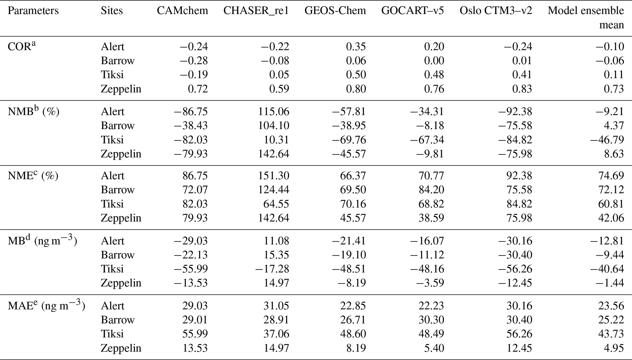
^a Correlative coefficient. ^b Normalized mean bias. ^c Normalized mean error. ^d Mean bias. ^e Mean absolute error.

3.2 Near-surface BC concentrations in the Arctic

Before analyzing the responses of Arctic BC to emission reductions, it is necessary to understand the spatiotemporal distribution of BC concentrations in the Arctic region. In this study, the months from May to October were defined as summer, and November to April were defined as winter due to the special geographical location of the Arctic (Aamaas et al., 2017).

Spatial distributions of Arctic near-surface BC concentrations in summer and winter simulated from each model are shown in Fig. S4. BC simulated by CHASER_re1 showed relatively high concentrations over the whole Arctic, followed by GEOS-chem and GOCART–v5, while those simulated by Oslo CTM3–v2 and CAMchem were lower. The difference in simulated BC concentrations between land and ocean was more obvious in summer than that in winter, especially for GEOS-chem and GOCART–v5. The mean BC concentrations from the ensemble models near the surface Arctic (66–90^∘ N) were 18.6 ng m⁻³ in summer and 16.6 ng m⁻³ in winter in 2010, respectively. Figure 2 shows that the BC concentrations over the polar sea ice region in winter were higher than those in summer. The coverage of the polar dome expanded more southward in winter (Bozem et al., 2019; Law and Stohl, 2007), allowing more BC from lower-latitudinal regions to be transported into the Arctic. Turbulent exchange and deposition were reduced during winter as the meteorological conditions in the Arctic were stable and dry (Bradley et al., 1992; Bozem et al., 2019; Law and Stohl, 2007). In addition, BC emissions in the EAS, EUR, and RBU regions showed obvious monthly changes with higher emissions from November to March as mentioned earlier (Sect. 2.1.1), leading to the relatively high BC concentrations over the polar sea ice region in winter. Over the terrestrial areas within the Arctic Circle, summer BC concentrations were higher than winter, especially in Siberia and Alaska, which were attributed to intense BC emissions from biomass burning over these areas from June to August (Fig. S3).

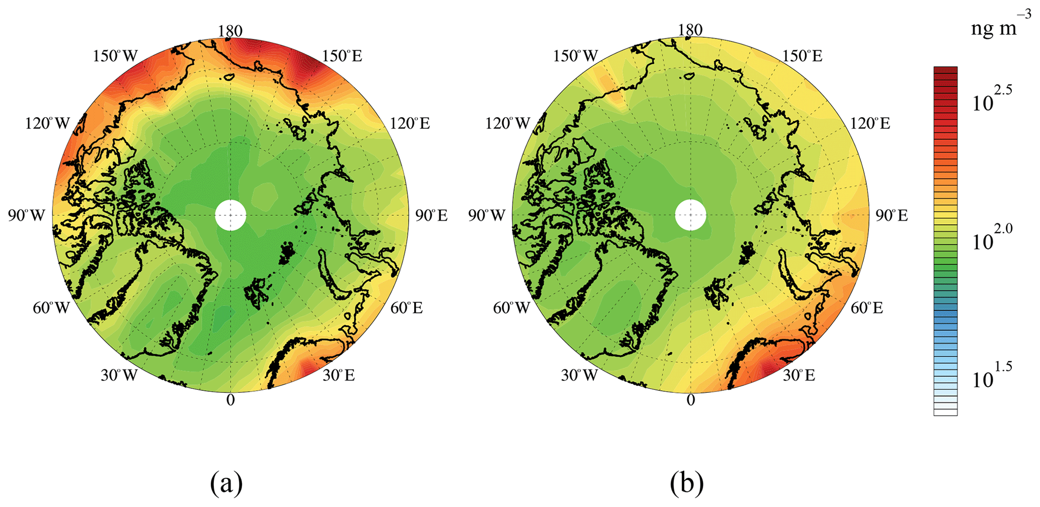
Figure 2 Spatial distribution of near-surface BC concentrations in (a) summer and (b) winter in the Arctic in 2010.

3.3 Response of Arctic BC to 20 % emission reductions

3.3.1 Contributions of regional emission reductions to the Arctic near-surface BC

The response of the Arctic near-surface BC to 20 % emission reductions from different source regions was analyzed through emission perturbation simulations. Figure 3 shows the spatial distribution of the response referred to above in summer and in winter of 2010 based on multi-model ensemble mean results. The source region contributions to the surface BC concentrations exhibited significant seasonal variability with higher values in winter. The BC emission reductions in EAS almost affected the whole Arctic, especially in winter, indicating the significance of the intercontinental transport of BC. The spatial distribution of the Arctic near-surface BC response to SAS emission reductions was similar to that of EAS, but the extent was much weaker. The emission reductions from EUR, NAM, and RBU mainly affected the local and nearby areas, which was generally consistent with the spatial pattern of emissions (Fig. 1). The contribution from MDE emission reductions was very little.

Figure 3 Spatial distribution of contribution of 20 % emission reductions in different source regions to Arctic near-surface BC in summer and in winter in 2010.

The monthly variations in the response of the Arctic near-surface BC concentrations to 20 % emission reductions from six source regions are presented in Fig. 4. Results from the ensemble simulations are averaged over the Arctic, covering latitudinal areas from 66^∘ N to the north pole. The emission reductions from the total six source regions were 329.6 Gg during May to October, lower than those of 411.9 Gg during November to April (Table 1). Correspondingly, the contributions of 20 % BC emission reductions from all six regions to Arctic monthly near-surface BC concentrations were 0.8–1.4 ng m⁻³ during May to October and 1.5–3.2 ng m⁻³ during November to April. Arctic sensitivities (Arctic concentration change per unit source region emission change) for BC typically maximized from December to February for EUR and RBU and from March to May for EAS and NAM (Shindell et al., 2008; AMAP, 2008). The enhanced sensitivity from December to May resulted from faster transport and slower removal during winter as the meteorological conditions in the Arctic were stable and dry (Law and Stohl, 2007). The results of deposition changes also proved this result well (Fig. S5). The wet deposition in summer was higher than that in winter, which was 7–13 times greater than dry depositions. Sharma et al. (2013) found that the Arctic region (north of 70^∘ N) was very dry during winter, with an average daily precipitation rate between 0 and 1 mm d⁻¹. Precipitation rates over some of the BC source regions such as Eurasia were at the same order of magnitude as the Arctic. Less wet deposition and a shallow boundary layer resulted in higher BC concentrations near the surface during winter. In the summertime, the Arctic region experienced 2 to 3 times higher precipitation rates as well as wet depositions of BC relative to wintertime, thus resulting in lower contributions to the near-surface BC concentrations.

Figure 4 Monthly mean reduced concentrations of the near-surface Arctic BC due to 20 % emission reductions from six source regions in 2010.

The annual contribution of 20 % emission reductions from EAS, EUR, MDE, NAM, RBU, and SAS to the Arctic near-surface BC concentrations reached 0.70, 0.54, 0.01, 0.20, 0.29, and 0.09 ng m⁻³ in 2010, respectively, totaling about 1.83 ng m⁻³. A simple linear interpolation suggested that the contribution of 100 % BC emissions from six regions to the Arctic near-surface BC concentrations was about 9.15 ng m⁻³ (5 times the contribution of 1.83 ng m⁻³). The annual mean Arctic near-surface BC concentration from the BASE simulation was about 18 ng m⁻³ in 2010. Thus, the impact of emissions from six regions on the Arctic near-surface BC was outstanding. It should be noted that the contributions from six regions only considered anthropogenic emissions, while the contribution from biomass burning was not included in the sensitivity experiments of HTAP2. It is known that wildfires in Far East of Russia and Alaska, USA, are important sources of BC in the Arctic region, especially in summer. Thus, the contributions from six regions to the Arctic BC should be even more dominant over the other regions by including biomass burning in RBU and NAM. The response of Arctic near-surface BC concentration was found to be strongest to the 20 % emission reductions from EAS, with a monthly contribution of 0.2–1.5 ng m⁻³, accounting for 16.8 %–49.0 % of the total reduced BC concentrations resulting from all six source regions (Fig. 4). On one hand, the BC emission reductions in EAS were the largest among the six source regions (Table 1). On the other hand, BC emission reductions in EAS can influence the Arctic lower troposphere via two pathways (Bozem et al., 2019; Stohl, 2006). BC from northern regions of EAS can enter into the polar dome of the Arctic in winter as the air masses have cooled during transport. BC from eastern regions of EAS uplifted fast due to convection, then followed by high-altitude transport in northerly directions. Radiative cooling eventually led to a slow descent into the polar dome area after air masses arrived in the high Arctic. It occurred both in summer and winter. In addition to EAS, BC emission reduction from EUR also showed significant impacts on the Arctic near-surface BC concentration, with a monthly contribution of 0.2–1.0 ng m⁻³, accounting for 20.1 %–49.0 % of the total reduced BC concentrations resulting from all six source regions (Fig. 4). Among the three regions in the Arctic Circle (i.e., EUR, NAM, and RBU), the EUR region had the largest BC emission reductions. Also, the relatively short distance between EUR and the Arctic made EUR the second most important source region to the Arctic. As for NAM and RBU, their 20 % emission reductions induced moderate reductions in the monthly Arctic near-surface BC concentrations by 0.1–0.3 and 0.1–0.7 ng m⁻³, respectively. The contribution of 20 % emission reductions from SAS to the Arctic near-surface BC concentrations was much lower than monthly contributions of 0.0–0.2 ng m⁻³ as a significant portion of BC originating from SAS accumulated in the upper troposphere (Sect. 3.3.2). Compared to the five source regions discussed above, the response of Arctic BC concentrations to emission reductions from MDE was negligible, owing largely to the low emissions there and long distance from the Arctic.

Figure S6 compares the contributions of 20 % emission reductions to Arctic near-surface BC concentrations simulated by different models. All five models showed similar monthly variations, of which CHASER_re1 simulated high BC concentrations compared to the other models due to slow aging speed (Sudo et al., 2015). All models showed the major source regions of Arctic BC from EAS, EUR, and RUB. NAM and SAS contributed moderately, while the contribution from MDE was negligible.

3.3.2 Contributions of regional emission reductions to the vertical BC profiles

To assess the contributions from various source regions to the BC profiles based on the model ensemble mean, the vertical stratification needed to be unified as most participating models had different vertical settings. Since CHASER had a relatively coarse vertical resolution of 32 layers, the other models were unified to the same vertical stratification, as detailed in Table S2.

As shown in Fig. 5, the contributions of regional emission reductions to BC exhibited strong vertical gradients over the Arctic. In general, the BC profiles displayed a bimodal pattern in summer, showing peaks at around 1.0–1.6 km a.s.l. (4th and 5th layers) and 8.0–8.9 km a.s.l. (13th and 14th layers), while in winter, the BC profiles showed a unimodal pattern with peaks around 0.6–1.6 km a.s.l. (3rd–5th layers). Long-range transport of air pollution may occur near the planetary boundary layer (Eckhardt et al., 2003; Stohl et al., 2002). High contributions in the low layers (e.g., 3rd–5th layers) were consistent with the height of the planetary boundary layer in the Arctic (Zhang et al., 2018; Cheng, 2011).

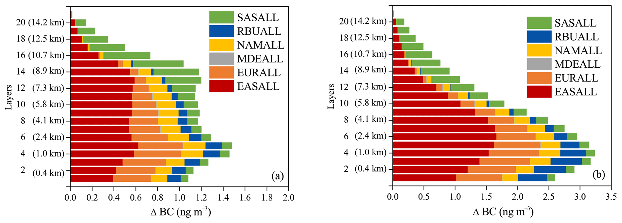
Figure 5 Contribution of 20 % emission reductions from six source regions to BC concentrations in different vertical layers (a) in summer and (b) in winter in the Arctic in 2010.

It has been summarized that there were several major transport pathways for BC into the Arctic troposphere (Stohl, 2006). (i) BC transported rapidly at a low level, followed by uplifting at the Arctic front when it is located far north. Significant deposition of BC in the Arctic occurs mostly north of 70^∘ N for this transport route. This transport route derived often from the high-BC-emission areas in northern EUR but seldom from the NAM and RBU. That was mainly due to the fact that the BC emissions exist at high enough latitudes in EUR, which can be north of the polar front. However, the BC emissions in NAM and RBU were concentrated south of the polar front (Fig. 1); thus BC emitted from these two regions cannot be easily transported into the Arctic through this pathway. (ii) Cold air masses into the polar dome transport at a low level. This pathway derived mainly from EUR and high-latitude areas of EAS during winter. The contribution of 20 % emission reductions from EUR to the Arctic BC concentrations peaked at around 1.0 km a.s.l., with a multi-model ensemble mean value of 0.4 ng m⁻³ in summer, while it peaked at a lower altitude of around 1.6 km a.s.l. with a value of 0.8 ng m⁻³ in winter. (iii) BC could also ascend south of the Arctic, followed either by high-altitude transport or by several cycles of upward and downward transport, and finally slowly descended into the polar dome due to radiative cooling. This was the frequent transport route from source regions such as NAM, RBU, and eastern EAS. The contribution from NAM and RBU to the Arctic BC peaked at about 1.6 km a.s.l. (0.2 ng m⁻³) and 1.0 km a.s.l. (0.2 ng m⁻³) in summer and peaked at about 1.0 km a.s.l. (0.3 ng m⁻³) and 0.4 km a.s.l. (0.5 ng m⁻³) in winter. The contribution from EAS including pathways ii and iii to the Arctic BC peaked at about 1.6 km a.s.l. (0.6 ng m⁻³) in summer and peaked at about 2.4 km a.s.l. (1.6 ng m⁻³) in winter. Matsui et al. (2011) pointed out that Asian anthropogenic air masses were measured most frequently in the upper troposphere, with median values of 20 ng m⁻³ (410 hPa) in April 2008 and 5 ng m⁻³ (353 hPa) in June–July 2008. In our analysis, the contribution of 20 % emission from EAS and SAS to BC in the Arctic was 1.4 ng m⁻³ (432 hPa) in April 2010 and 0.7 ng m⁻³ (375 hPa) in June–July 2010. If the contribution was linearly interpolated, the contribution of 100 % emission from EAS and SAS to BC in the Arctic would be about 7 ng m⁻³ (432 hPa) in April and 3.5 ng m⁻³ (375 hPa) in June–July in 2020. In general, our results were of the same magnitude as those of Matsui et al. (2011). The contribution from MDE was negligible.

As shown in Fig. 5, BC can also be transported into the upper troposphere of the Arctic. Air masses preferably kept their potential temperature almost constant during transport as the atmospheric circulation can be well described by adiabatic motions in the absence of diabatic processes related to clouds, radiation, and turbulence. The potential temperature was low within the polar dome area, and thus only air masses that experienced diabatic cooling were able to enter the polar dome (Stohl, 2006). That is to say, the air masses from SAS and low-latitude regions of EAS could not easily penetrate the polar dome but can be lifted and transported to the Arctic in the middle and upper troposphere along the isentropes (AMAP, 2011; Barrie, 1986; Law and Stohl, 2007; Stohl, 2006). This agreed well with the previous study of Koch and Hansen (2005) and Stohl (2006). The contribution from SAS to the Arctic BC concentrations peaked at about 9.7 km a.s.l. (0.4 ng m⁻³) in summer and 9.7 km a.s.l. (0.5 ng m⁻³) winter. This was also consistent with the vertical profiles of BC shown in Stjern et al. (2016). The polar dome boundary was variable in time and space and was not zonally symmetric. The range of the polar dome expanded southward to about 40^∘ N over Eurasia in winter as the temperature difference in different latitudes became smaller (Bozem et al., 2019; Law and Stohl, 2007), resulting in the contribution of EAS to the Arctic BC concentrations in the upper troposphere only peaking in summer in the 13th layer (8.0 km a.s.l.), with a value of 0.6 ng m⁻³.

3.3.3 Contributions of emission reductions to BC in different latitudinal bands

To further analyze the response of the Arctic BC concentrations to emission reductions in six source regions in HTAP2, the contribution of 20 % emission reductions to BC concentrations at different latitudes of the Arctic were calculated (Figs. 6 and 7). In regard to the different horizontal resolution of participating models, the Arctic region (66–90^∘ N) was divided into eight latitudinal bands with a 3^∘ interval, which was based on the coarsest resolution of all models.

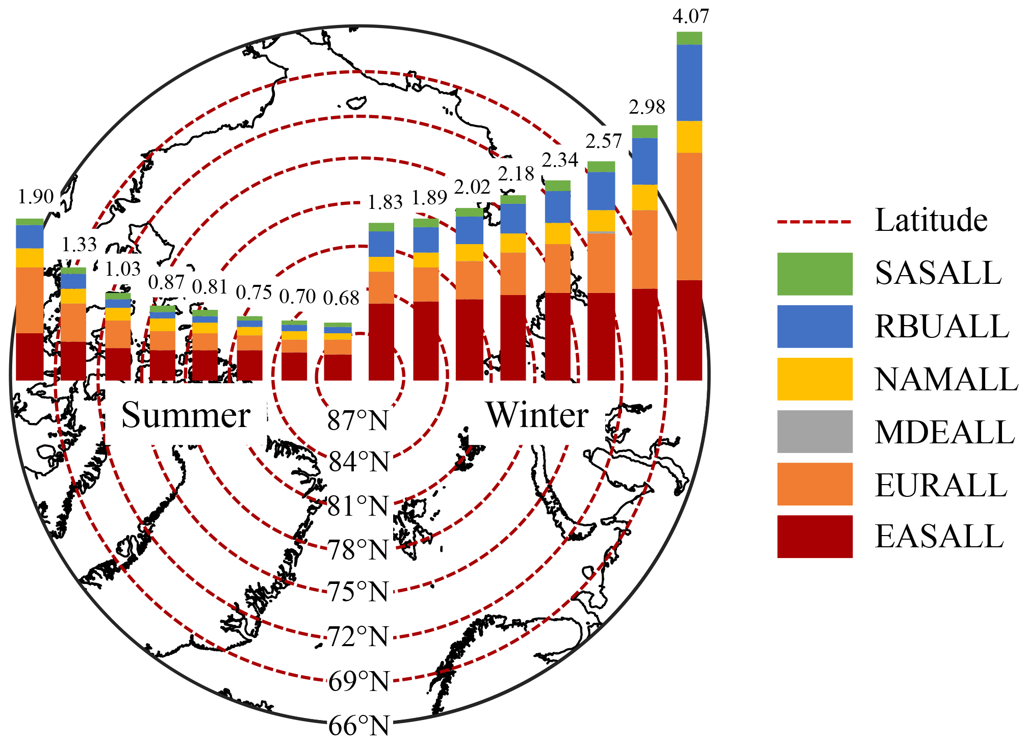
Figure 6 Contributions of 20 % emission reductions in different regions to near-surface BC concentrations in each latitudinal band of the Arctic. The results of summer and winter correspond to the left and right panel in the figure.

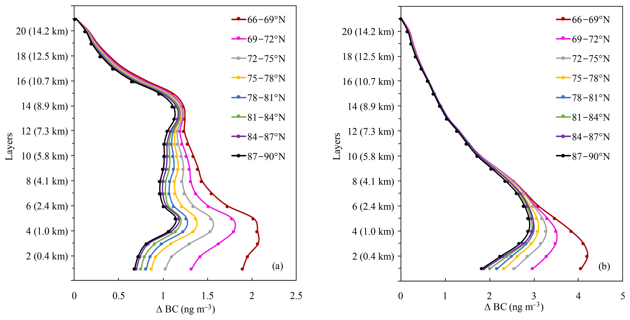
Figure 7 Contributions of 20 % emission reductions from all six source regions to the vertical BC concentrations of the Arctic in different latitude bands vary with vertical layers in (a) summer and (b) winter in 2010.

The response of the Arctic BC concentrations to emission reductions in six source regions became weaker with the increase in the latitude due to the continuous loss of BC during transport (e.g., dry and wet depositions) (Fig. 6). The difference in contributions between two adjacent latitudinal bands became smaller closer to the north pole. The contributions of 20 % emission reductions to the Arctic BC concentrations near the surface were the highest between 66–69^∘ N both in summer (1.9 ng m⁻³) and winter (4.1 ng m⁻³), which were 1.4–2.8 times higher than the other latitudinal bands.

The contributions from EAS and EUR were higher than those from the other four regions in each latitudinal band. In detail, the contributions from EUR (0.8 ng m⁻³ in summer and 1.5 ng m⁻³ in winter) were higher than those from EAS (0.6 ng m⁻³ in summer and 1.2 ng m⁻³ in winter) in the latitudinal band of 66–69^∘ N as the BC concentrations near the surface there were more sensitive to the local emission sources. In contrast, the latitudinal contributions from EAS (0.3–0.4 ng m⁻³ in summer and 0.9–1.1 ng m⁻³ in winter) were higher than those from EUR (0.2–0.4 ng m⁻³ in summer and 0.4–0.9 ng m⁻³ in winter) in the other high-latitudinal bands where long-range transport played the dominant role.

The downward trends of the response of the Arctic near-surface BC to emission reductions with the increase in latitude from EUR and RBU were more obvious than those of other regions (Fig. 6). Dry and wet depositions of BC decreased with the increase in transport distance, and the decreasing rates became slower (Fig. S7). The changes in dry and wet depositions caused by emission reductions from EUR and RBU were still obvious in the Arctic region (66–90^∘ N), while depositions caused by emission reductions from the other regions tended to be gentle (Fig. S7). This explains why the contribution from EAS to BC at different latitudes remained almost constant, while that from EUR and RBU decreased obviously from lower latitudes to the Arctic pole.

Figure 7 further depicts the response of the vertical Arctic BC profiles in different latitudinal bands to 20 % emission reductions. The contributions of eight latitudinal bands showed a typical bimodal pattern in summer with peaks at 0.6–1.6 km a.s.l. (3rd–5th layers) and 8.0–8.9 km a.s.l. (13th and 14th layers), while the contribution displayed a single peak at 0.4–1.0 km a.s.l. (2nd–4th layers) in winter. Similar to Sect. 3.3.2, the peak value of the contribution at the low layers was due to the transport of EAS, EUR, NAM, and RBU emission reductions to the Arctic through different pathways both in summer and winter. The peak value in the high layers in summer was due to the transport of EAS and SAS. However, a high contribution of 20 % emission reductions to BC concentrations in SAS was found in the high layers, while the contribution was low in other regions, leading to a single peak in winter. The statistical results of SAS indicated that the contribution in the vertical appeared in one peak in the 15th layer (9.7 km a.s.l.), with values of 0.45 and 0.48 ng m⁻³ in summer and winter, respectively (Fig. S8).

The same as the whole Arctic region (Sect. 3.3.1 and 3.3.2), the contributions of 20 % emission reductions to BC concentrations in eight latitude bands were higher in winter than in summer, whether near the surface or in the vertical. The contribution of 20 % emission reductions from all six source regions to BC concentrations in eight latitude bands of the Arctic near the surface was 0.7–1.9 ng m⁻³ in summer and 1.8–4.1 ng m⁻³ in winter, respectively (Fig. 6). The high BC peak at around 0.6–1.6 km a.s.l. (3rd–5th layers) was 1.1–2.1 ng m⁻³ in summer and 2.9–4.2 ng m⁻³ in winter (Fig. 7).

3.4 Benefit of BC emission reductions on the decrease in Arctic temperature

The impact of BC emission reductions on decreasing the Arctic (60–90^∘ N) surface temperature was assessed by using ARTP (See methods in Sect. 2.2). Aerosol effects, BC deposition on snow, and BC semi-direct were considered in the calculation of ARTP (Aamaas et al., 2017). As shown in Fig. 8, the response of Arctic surface temperature to emission reductions was the most significant at the timescale of 10 years and then gradually decreased with the passage of time. For each source region, the Arctic temperature response was significantly higher in winter than in summer as ARTP was seasonally dependent, with higher values in the colder seasons. Obviously, the Arctic surface temperature benefited the most from BC emission reductions from EAS, with more than 300 and 660 µK decreases in summer and winter after 10 years, respectively. The influences of EUR and NAM emission reductions on the temperature decrease were similar in summer, reaching about 3–90 µK after 10, 20, 50, and 100 years. However, in winter, the influence of emission reductions from NAM on temperature decrease (8–200 µK) was weaker than that from EUR (14–370 µK). This was mainly because the difference in ARTPs between EUR and NAM was not obvious compared with the difference in emission reductions from NAM and EUR in summer and winter. The responses of the temperature decrease to emission reductions from RBU were 9–20 µK in summer and 4–100 µK in winter after 10–100 years, respectively, which were smaller than that from EUR and NAM. This can be explained by the low BC emission reductions from RBU (Table 1). The response of the temperature decrease to emission reductions from SAS in winter (10–320 µK) was similar to that from EUR, while this response in summer (8–230 µK) was more than twice that of EUR. Although the ARTP of EUR was higher than that of SAS, the BC emission reductions from SAS were much higher than those from EUR, and the difference between emission reductions from the two regions was more obvious in summer (Table 1). In spite of the higher Arctic temperature response to EAS than SAS in the target year of this study, a number of studies have shown that BC emissions in South Asia were increasing in recent years (Sahu et al., 2008; Paliwal et al., 2016; Sharma et al., 2019), while the emissions of East Asia were exhibiting a downward trend, especially from China (Chen et al., 2016); thus more attention should be given to the impact assessment of South Asia on the Arctic in the future. The minimum temperature response was found from MDE due to the least emission reductions and small ARTP.

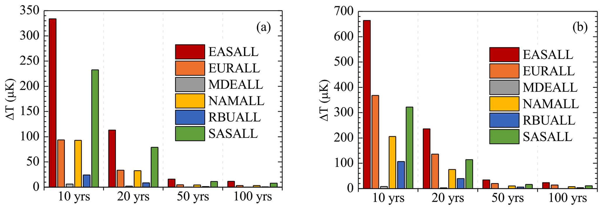
Figure 8 Arctic surface temperature response to 20 % regional BC emission reductions in (a) summer and (b) winter after 10, 20, 50, and 100 years.

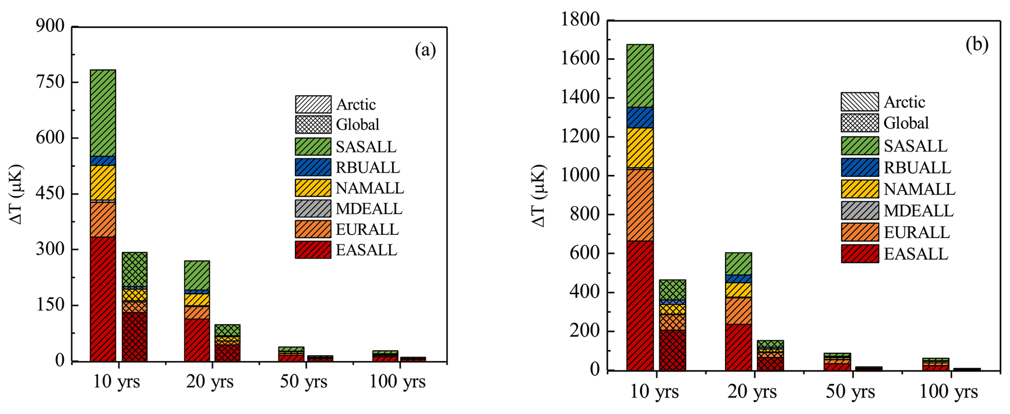
Figure 9 Global and Arctic surface temperature responses to 20 % regional BC emission reductions in (a) summer and (b) winter after 10, 20, 50, and 100 years.

In addition, the impacts of BC emission reductions from six source regions on the Arctic and global surface temperature were compared in this study (Fig. 9). Due to the BC emission reductions from the six source regions, the surface temperature in the Arctic decreased 27–780 µK in summer and 61–1675 µK in winter after 10, 20, 50, and 100 years, which were greater reductions than the global values of 10–290 µK in summer and 16–470 µK in winter. It can be seen that the difference in the temperature response between the Arctic and the globe was more obvious in winter. Overall, the response of the Arctic surface temperature was more sensitive to emission perturbation than the globe surface temperature.

It should be noted that the estimation of temperature response was subject to large uncertainties for the following reasons. On the one hand, even though the HTAP2 emissions database was all constructed by bottom-up methods, the different inventories and spatiotemporal distributions were constructed with sub-regional (country, state, county, or province level) activity data and emission factors, which lead to inconsistencies at the borders between two adjacent inventories. Version 5 of Evaluating the Climate and Air Quality Impacts of Short-Lived Pollutants (ECLIPSEv5; http://eclipse.nilu.no, last access: 3 June 2021) estimated a 2010 emission inventory that also serves as a reference point for all projections (Janssens-Maenhout et al., 2015). At the global level, a relatively good agreement was found with small relative emission differences compared with the ECLIPSEv5 emission inventory for the aggregated sectors in 2010. However, larger differences of 29 % between HTAP2 and ECLIPSEv5 emissions were present for BC since ECLIPSEv5 relied on provincial statistics for China, which resulted from higher coal consumption than reported national statistics. Hoesly et al. (2018) provided a sectoral and gridded historical (1750–2014) anthropogenic emission inventory for use in the Coupled Model Intercomparison Project Phase 6 (CMIP6). The amount of global BC anthropogenic emissions was 7.7 Tg yr⁻¹ in 2010 from the CMIP6 emissions, which was larger than that from HTAP2 emissions (5.5 Tg yr⁻¹). This was mainly because the BC emissions of energy, transportation, and international shipping sectors of CMIP6 were higher than those of HTAP2.

On the other hand, the time evolution of R_T, a parameter in the calculation of ARTP, was also one factor causing the uncertainty in temperature response calculation. This impulse response function was only based on one coupled atmosphere–ocean climate model, GISS-ER, in this study, while Olivié and Peters (2013) have found a spread in the GTP value of BC of about −60 % to +80 % for time horizons of 20 years due to variability in R_T among various models. However, the uncertainty in R_T was less relevant for the regional patterns. Forcing-response coefficients did not exist on a seasonal basis since emissions occurring during the Northern Hemisphere summer and winter seasons were differentiated (Aamaas et al., 2017). Hence, the seasonal differences presented here in the ARTP values were not due to potential differences in the response sensitivities but due to differences in the RF. The temperature response will vary by species and location, such as between land surface and ocean surface. These differences are not accounted for in this study, but the increased efficacy in the RCS matrix towards the NH can be partly attributed to a larger land area fraction in the NH (Shindell et al., 2015). Besides, recent studies have found that the positive radiation budget of BC is largely compensated for by rapid atmospheric adjustment. This means that the responses of surface temperatures to BC tend to be weaker than expected (Stjern et al., 2017; Takemura and Suzuki, 2019).

Although the HTAP2 emissions database contains uncertainties, and ARTP calculations are simplifications, these emission metrics are useful, simple, and quick approximations for calculating the temperature response in the different latitude bands for emissions of BC. It should be noted that the estimated responses of Arctic surface temperature to 20 % emission reductions were only valid for the comparison among different source regions but cannot be used to reflect the actual change in temperature. On the one hand, in reality, not all emissions sectors of a specific source region can be reduced by 20 % at the same time. On the other hand, there were many other factors (e.g., greenhouse gases, sea ice coverage) that can affect the temperature change in the Arctic besides BC.

4 Conclusions

CAMchem, CHASER_re1, GEOS-Chem, GOCART, and Oslo CTM3 in the HTAP2 experiment were used in this study to estimate the responses of Arctic BC to multi-region emission reductions in 2010. Six regions (e.g., EAS, EUR, MDE, RBU, NAM, and SAS) were selected as the source regions, and the Arctic was the receptor region. HTAP2 set up the base scenario with all BC emissions and also simulated BC concentrations with 20 % reduction in anthropogenic emissions. The ARPT was further used to calculate the benefit of BC emission reductions to the decrease in Arctic temperature.

The statistical results of 20 % BC emission reductions showed that emission reductions in EAS were the largest, with values of 355.6 Gg yr⁻¹, followed by SAS (232.5 Gg yr⁻¹), EUR (65.3 Gg yr⁻¹), NAM (62.2 Gg yr⁻¹), RBU (18.6 Gg yr⁻¹), and MDE (5.3 Gg yr⁻¹). The BC emission reductions in the EAS, EUR, and RBU were higher from November to March.

The temporal variations in simulations from different models were relatively consistent as the correlations of the simulated BC concentrations among different models ranged from 0.33 to 0.98. However, the simulated BC concentrations did not agree so well with observations at monitoring sites, except Zeppelin. In order to reduce the difference in simulation performance of each model in different areas of the Arctic, the model ensemble mean was used for analysis.

The contribution of 20 % BC emission reductions from EAS, EUR, MDE, NAM, RBU, and SAS to the Arctic near-surface BC concentrations reached 0.70, 0.54, 0.01, 0.20, 0.29, and 0.09 ng m⁻³, respectively. Correspondingly, the reduced column BC loadings from the six regions over the Arctic were 8521.7, 2789.1, 28.8, 1762.1, 998.6, and 3640.2 ng m⁻², respectively.

The response of Arctic near-surface BC concentrations to 20 % emission reductions from EAS and EUR was larger than the other four source regions, with a monthly value of 0.2–1.5 and 0.2–1.0 ng m⁻³, accounting for 16.8 %–49.0 % and 20.1 %–49.0 % of the total contributions from all six regions, respectively. The BC profiles displayed a bimodal pattern in summer with peaks at around 1.0–1.6 km a.s.l. (4th and 5th layers) and 8.0–8.9 km a.s.l. (13th and 14th layers), while the BC profiles showed a unimodal pattern with peaks around 0.6–1.6 km a.s.l. (3rd–5th layers) in winter.

The response of Arctic BC to emission reductions from source regions in winter was higher than that in summer. The contributions of 20 % emission reductions to the Arctic BC concentrations near the surface were the highest between 66–69^∘ N both in summer (1.9 ng m⁻³) and winter (4.1 ng m⁻³) and became weaker with the increase in the latitude.

The response of Arctic temperature to BC emission reductions was the most significant at the timescale of 10 years and then gradually decreased with the passage of time. The Arctic had benefited the most from emission reduction in EAS, with more than 300 and 660 µK decreases in summer and winter after 10 years, respectively. The Arctic temperature response was more sensitive to the whole globe with regard to the same emission perturbation. The estimation of temperature response was subject to large uncertainties due to the uncertainties in the calculation of ARTP and emissions of BC in source regions.

Overall, this study provided insights on the source regions and seasonal contributions of Arctic BC from the most recent international ensemble modeling efforts. The discrepancy between model results and observations and the spread among different HTAP models may be attributed to various factors such as emissions in the remote Arctic, physical parameterizations, and convection and deposition processes. This would subsequently result in large uncertainties in the climatic effects of air pollutants. More observation sites for the typical transport pathways from source regions to the Arctic should be planned to improve the model capability of simulating the transport behavior of black carbon.