the Creative Commons Attribution 4.0 License.
the Creative Commons Attribution 4.0 License.
 | 08 Jun 2021
Differences in the quasi-biennial oscillation response to stratospheric aerosol modification depending on injection strategy and species
Henning Franke
Ulrike Niemeier
Daniele Visioni
A known adverse side effect of stratospheric aerosol modification (SAM) is the alteration of the quasi-biennial oscillation (QBO), which is caused by the stratospheric heating associated with an artificial aerosol layer. Multiple studies found the QBO to slow down or even completely vanish for point-like injections of SO2 at the Equator. The cause for this was found to be a modification of the thermal wind balance and a stronger tropical upwelling. For other injection strategies, different responses of the QBO have been observed. A theory which is able to explain those differences in a comprehensive manner has not yet been presented. This is further complicated by the fact that the simulated QBO response is highly sensitive to the used model even under identical boundary conditions. Therefore, within this study we investigate the response of the QBO to SAM for three different injection strategies (point-like injection at the Equator, point-like injection at 30∘ N and 30∘ S simultaneously, and areal injection into a 60∘ wide belt along the Equator). Our simulations confirm that the QBO response significantly depends on the injection location. Based on the thermal wind balance, we demonstrate that this dependency is explained by differences in the meridional structure of the aerosol-induced stratospheric warming, i.e., the location and meridional extension of the maximum warming. Additionally, we also tested two different injection species (SO2 and H2SO4). The QBO response is qualitatively similar for both investigated injection species. Comparing the results to corresponding results of a second model, we further demonstrate the generality of our theory as well as the importance of an interactive treatment of stratospheric ozone for the simulated QBO response.
- Article
(16745 KB) - Full-text XML
-
Supplement
(1236 KB) - BibTeX
- EndNote


Stratospheric aerosol modification (SAM) by the artificial injection of sulfur dioxide (SO2) into the lower stratosphere is currently widely discussed as a potential measure against global warming for the case of unmitigated greenhouse gas (GHG) emissions. It would basically mimic the processes after a large stratospheric volcanic eruption, resulting in an enhancement of the natural stratospheric sulfate aerosol layer. Since sulfate aerosols backscatter incoming shortwave radiation (ISR), this enhancement of the stratospheric sulfate aerosol layer causes a negative radiative forcing (RF) on the Earth system, which would counteract the tropospheric warming caused by increasing atmospheric GHG concentrations.
Besides backscattering ISR, sulfate aerosols also absorb parts of the outgoing tropospheric longwave radiation (OTLR) and the incoming near-infrared radiation (NIRR). The absorption of OTLR and NIRR causes a significant warming of the lower tropical stratosphere (e.g., Heckendorn et al., 2009; Ferraro et al., 2011). This warming has important consequences for stratospheric dynamics, including the quasi-biennial oscillation (QBO). The QBO is a zonally symmetric oscillation of the zonal wind in the tropical stratosphere with an average period of approximately 28 months (Baldwin et al., 2001; Naujokat, 1986). It is characterized by an alternating downwelling of westerly and easterly winds from the upper stratosphere, above 5 hPa, into the tropopause region, where these wind patterns are rapidly attenuated (Baldwin et al., 2001; Holton, 2004). The QBO has an impact on tropospheric winds (Garfinkel and Hartmann, 2011) and precipitation (Seo et al., 2013), as well as on the stratospheric transport to the extratropics (Plumb and Bell, 1982; Punge et al., 2009) and the polar vortex (Holton and Tan, 1980). After the major eruption of Mt. Pinatubo in June 1991, the lower stratosphere warmed by about 3 K, which led to a prolonged QBO westerly phase in the lower stratosphere (Labitzke, 1994), very likely due to an increased tropical upwelling induced by the aerosol warming (Giorgetta et al., 2011, Henning Franke and Marco Giorgetta, personal communication, 2020).
Multiple studies revealed that the QBO could also be heavily perturbed during a potential deployment of SAM (e.g., Aquila et al., 2014; Richter et al., 2017; Tilmes et al., 2018; Niemeier et al., 2020). For equatorial point injections, Aquila et al. (2014) obtained a prolonged or even permanent QBO westerly phase, depending on the injection rate. They attributed these modifications of the QBO basically to two physical mechanisms: a modification of the thermal wind balance due to the aerosol-induced warming of the lower tropical stratosphere and an acceleration of the tropical upwelling as a response to this warming, which decelerates the downward propagation of the QBO. Niemeier and Schmidt (2017) and Richter et al. (2017) further confirmed these results with other models.
Together with equatorial point injections, a modification of the QBO has been also noticed for other injection strategies. Niemeier and Schmidt (2017) obtained a significantly prolonged westerly phase of the QBO for an injection into a zonal belt along the Equator ranging from 30∘ N to 30∘ S with an injection rate of 10 Tg(S) yr−1 but weaker than for an equatorial point injection with the same injection rate. For point-like injections in the extratropics, the QBO response to SAM is also different. Richter et al. (2017) showed that the QBO speeds up instead of slowing down for point-like injections at 15∘ N, 15∘ S, 30∘ N, and 30∘ S, testing an injection rate of 6 Tg(S) yr−1. The root cause of this acceleration was not finally determined, despite a detailed analysis of the 2∘ N–2∘ S zonal mean momentum budget. Tilmes et al. (2018) analyzed a simultaneous injection at two points at 15∘ N and 15∘ S for two different injection heights with injection rates of 12 and 16 Tg(S) yr−1. Within their simulations, the QBO slightly slows down but with a prolonged easterly phase within the lower stratosphere instead of a prolonged westerly phase as for equatorial point injections. They argue that the short simulation period and the low vertical resolution of their model may be a reason for these contradictory results.
Additionally, Niemeier et al. (2020) showed that the simulated QBO response to SAM may be very sensitive to the used model itself by comparing two models (MAECHAM5-HAM and WACCM-110L) using the same model setup and injection protocol. Both models showed a qualitatively similar QBO response to SAM but quantitatively much stronger in WACCM-110L. The authors assumed differences in the vertical residual velocities in the tropics, which are also evident in a simulation without SAM, as the main cause of differences. Since the models used in the aforementioned studies as well as their specific setup vary significantly, the comparability of their results is consequently reduced. This further complicates the search for a comprehensive explanation of the at least partly contradictory QBO response to different injection locations.
To overcome this limitation, in this study we investigate the QBO response to three different injection locations for the same models as used by Niemeier et al. (2020) but with a different model setup in one case (see model description in Sect. 2). Both models followed the experimental protocol of the GeoMIP6 test bed experiment accumH2SO4 (Weisenstein and Keith, 2018) to compare the different efficiencies of SO2 and H2SO4. Since multiple studies found that the forcing efficiency decreases significantly with increasing injection rates of SO2 (e.g., Heckendorn et al., 2009; English et al., 2012; Niemeier and Timmreck, 2015; Vattioni et al., 2019), the direct injection of gaseous H2SO4 instead of SO2 has been suggested as a potential alternative (Pierce et al., 2010; Benduhn et al., 2016). For both models, we tested an injection into a zonal belt along the Equator ranging from 30∘ N to 30∘ S and a simultaneous point-like injection at 30∘ N and 30∘ S, and for one model we additionally tested an equatorial point injection. Unlike previous studies, we aim for an advanced understanding of the dynamical mechanisms which lead to the SAM-induced modification of the QBO for different injection locations. We will in particular focus on the modification of thermal wind balance by explicitly studying the SAM-induced modification of the meridional temperature gradient within the stratosphere, which was not done so far.
In Sect. 2, the models used in this study as well as the performed simulations are described. The results are structured as follows. In Sect. 3, we investigate the dependency of the QBO response to the injection location, rate, and species in our first model (MAECHAM5-HAM). Thereby, we give the theoretical explanation of the different responses to SAM – focusing on the modification of thermal wind balance – in Sect. 3.1.3. In Sect. 4, we then compare the SAM-induced modification of the QBO observed in MAECHAM5-HAM to that observed in CESM2(WACCM). This study ends with a discussion and a conclusion of the main findings in Sect. 5.
2.1 MAECHAM5-HAM
MAECHAM5 is the middle atmosphere version of the spectral general circulation model (GCM) ECHAM5 (Roeckner et al., 2003; Giorgetta et al., 2006; Roeckner et al., 2006). It simulates the evolution of atmospheric dynamics by numerically solving prognostic equations for temperature, surface pressure, vorticity, and divergence in terms of spherical harmonics. The different phases of water as well as tracers are transported within the model using a flux-form semi-Lagrangian transport scheme (Lin and Rood, 1996). Details on ECHAM5 can be found in Roeckner et al. (2003). MAECHAM5 has a vertical domain which extends from the surface up to 0.01 hPa while being resolved by 90 sigma-pressure levels. Additionally, it accounts for the momentum flux deposition of unresolved gravity waves (GWs) originating from the troposphere via a parameterization following Hines (1997a, b); its implementation into MAECHAM5 is described by Manzini et al. (2006). Therefore, MAECHAM5 internally generates a QBO in the tropical stratosphere (Giorgetta et al., 2006). For this study, MAECHAM5 was used with a spectral truncation at wave number 42 (T42), resulting in a horizontal Gaussian grid with 64 × 128 grid boxes with a size of 2.8 per grid box.
MAECHAM5 was interactively coupled to the prognostic modal aerosol microphysical model HAM (Stier et al., 2005), which is based on the microphysical core M7 developed by Vignati et al. (2004). HAM calculates aerosol microphysical processes like nucleation, accumulation, condensation, and coagulation as well as the sulfate aerosol depletion via sedimentation and deposition (Stier et al., 2005). In this setup of HAM, a simple stratospheric sulfur chemistry is applied in the stratosphere, which uses prescribed monthly oxidant fields and photolysis rates of, inter alia, ozone, OH, and NOx (Timmreck, 2001; Hommel and Graf, 2011). Therefore, the impact of SAM on stratospheric ozone is not simulated within MAECHAM5-HAM. Within this stratospheric HAM version, apart from the injected SO2 or H2SO4, only natural sulfur emissions are taken into account. These simulations use the model setup described in Niemeier et al. (2009) and Niemeier and Timmreck (2015), where more details can be found. The HAM aerosol model couples back to the dynamics by the aerosol optical properties in the shortwave, longwave, and near-infrared range, which enter the radiative transfer scheme in MAECHAM5 and thus influence the temperature. Consequently, the interactive modification of the QBO is simulated within MAECHAM5-HAM, which will be hereafter referred to as ECHAM.
2.2 CESM2(WACCM)
The Community Earth System Model version 2 (release 2.1) in the Whole Atmosphere Community Climate Model version CESM2(WACCM6) is a state-of-the-art fully coupled climate model, which is also used in the new CMIP6 simulations (Gettelman et al., 2019). It uses 72 vertical layers up to about 150 km and a 0.9∘ in latitude by 1.25∘ in longitude horizontal grid. WACCM6 includes convective, frontal, and orographic sources of GWs, which propagate to drive the circulation of the middle atmosphere, including the QBO.
Although the standard version of WACCM6 uses comprehensive chemistry from the troposphere to the lower thermosphere, the version used here only simulates middle atmospheric (stratosphere, mesosphere and lower thermosphere) chemistry, with 98 simulated chemical species. Sulfate aerosols are treated using the Modal Aerosol Model (MAM4) as described in Liu et al. (2012, 2016) but with some modifications to change the mode widths and to the capabilities of sulfate aerosol to grow into the larger mode; an explanation of this and an evaluation of its capabilities in simulating volcanic aerosols after Pinatubo is given in Mills et al. (2016, 2017). CESM2(WACCM) will be hereafter referred to as CESM.
2.3 Simulations
The experimental setup of the simulations performed in this study is in accordance with the proposal of the GeoMIP6 test bed experiment accumH2SO4 (Weisenstein and Keith, 2018) for both models. In all simulations, the sea surface temperature (SST) and the sea ice concentration (SIC) were set to monthly climatological values of the period 1988 to 2007 out of the AMIP SST data set following the experimental setup in Butchart et al. (2018). The GHG concentrations and the concentrations of ozone-depleting substances (ODSs) are taken from the SSP5-8.5 scenario of ScenarioMIP (O'Neill et al., 2016) for the year 2040. This combination of GHG and SST forcing allows us to approximately mimic the surface cooling that would be produced by the sulfate layer, while having a consistent surface field for all models and thus removing the source of uncertainty derived from differences in the simulated cooling amongst models. Due to their coarse horizontal resolution, the used models are not able to simulate the rapid initial formation of accumulation mode sulfate particles (AM−SO4) after the injection of H2SO4. Therefore, the injection of H2SO4 is modeled as a direct injection of an AM−SO4 population with a mode radius of 0.075 µm and a standard deviation of 1.59 in ECHAM and a mode radius of 0.1 µm and a standard deviation of 1.5 in CESM, both following the proposal of accumH2SO4 (Weisenstein and Keith, 2018).
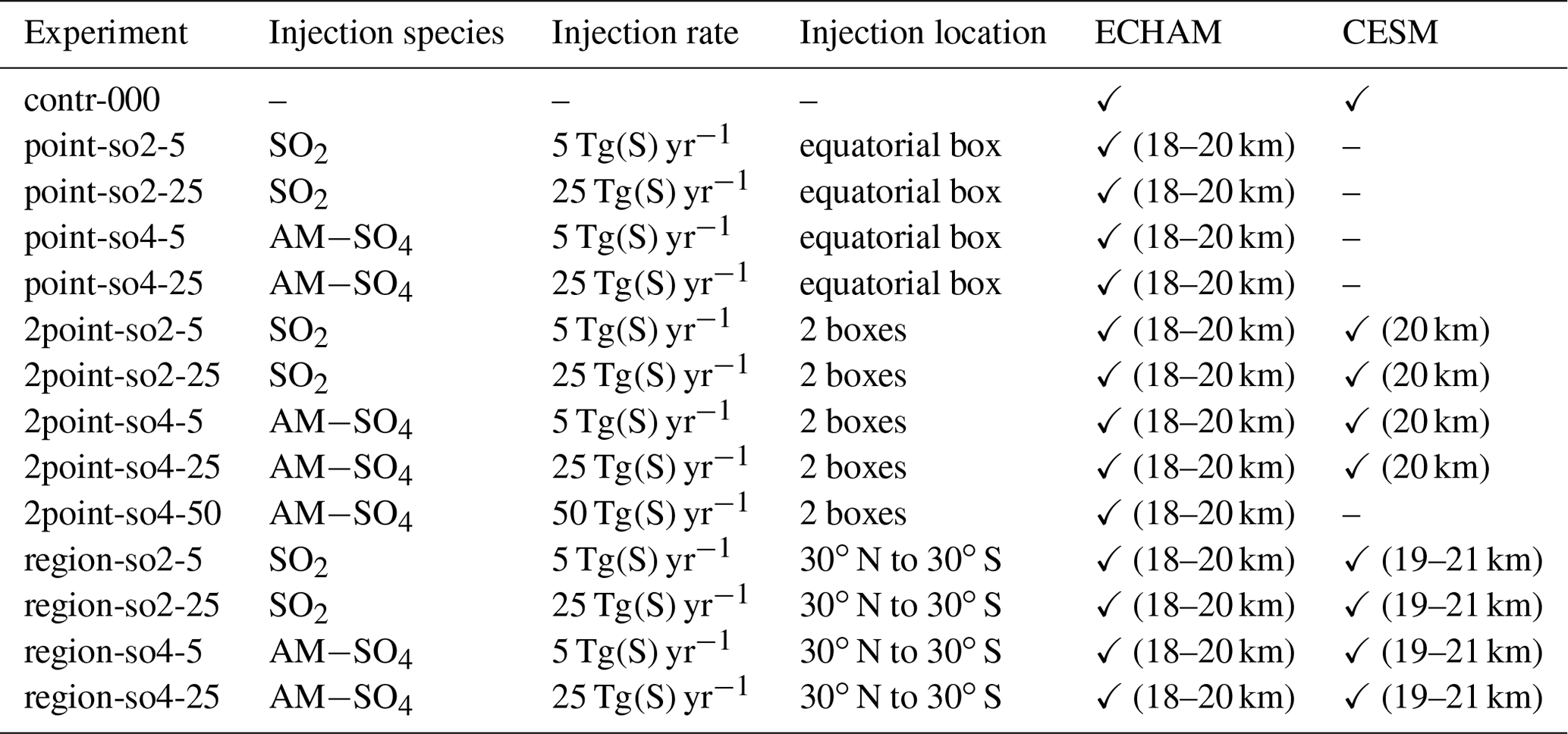
With ECHAM, three different injection strategies have been simulated for both injection species (SO2 and AM−SO4): an injection into one single grid box centered at 1.4∘ N, 180∘ E (termed point); a simultaneous injection into two grid boxes centered at 29.3∘ N, 180∘ E and 29.3∘ S, 180∘ E (termed 2point); and an injection into a zonally symmetric belt from 30∘ N to 30∘ S along the Equator (termed region). The injections took place in three adjacent model layers at a height between 18 and 20 km. With CESM, only the 2point and region injections have been simulated. The point injection strategy is not part of the accumH2SO4 experimental protocol and was, therefore, not performed by CESM. For the 2point injections, the injections took place in a single model layer at 20 km, while for the region injections the injections took place between 19 and 21 km. All injection scenarios have been simulated with two different injection rates for both models: 5 and 25 Tg(S) yr−1, as given by the accumH2SO4 protocol. The injection rate is the total amount of sulfur that is injected globally per year; for example, in the 2point injections with an injection rate of 25 Tg(S) yr−1, both injection points have an injection rate of 12.5 Tg(S) yr−1. For the 2point injection of AM−SO4 with ECHAM, an additional simulation with an injection rate of 50 Tg(S) yr−1 has been performed. An overview of all performed simulations and their setups can be found in Table 1.
All simulations were performed for a period of 10 years. If not otherwise stated, the results presented in this study are averaged over the last 8 years of the respective simulation, since Visioni et al. (2019) showed that the artificial stratospheric sulfate layer has reached equilibrium already by the third year of deployment. All anomalies presented in this study have been calculated with respect to the control simulation (termed contr-000) of the corresponding model. The control simulations were performed with the same SST, SIC, GHG, and ODS specifications like the SAM simulations but without any artificial injection of some sulfur species.
Table 1Setup of all performed simulations. The point injections have been performed in a single equatorial grid box centered at 1.4∘ N, 180∘ E; the 2point injections have been performed in two boxes centered at 29.3∘ N, 180∘ E and 29.3∘ S, 180∘ E; and the region injections have been performed in a belt along the whole Equator, ranging from 30∘ N to 30∘ S. The injection rate is the total amount of sulfur that is injected globally per year. Check marks indicate whether the experiment was performed for the according model, while values in parenthesis after the check marks indicate the injection altitude.
ECHAM simulates the QBO well in the control simulation (Fig. 1a–c), where it has a period of roughly 32 months, which is slightly longer than the observed period of approximately 28 months (Naujokat, 1986). Artificial sulfur injections may lead to a substantial modification of the QBO compared to the control simulation in ECHAM, depending on the injection strategy, injection species, and injection rate (Fig. 1d–i). The equatorial point injections lead to the most significant modification of the QBO compared to the other injection strategies: while an injection of SO2 with an injection rate of 5 Tg(S) yr−1 (Fig. 1d) already leads to a drastic slowdown of the QBO with a prolonged lower-stratospheric westerly phase, the QBO is locked in a constant lower-stratospheric westerly phase for a SO2 injection with an injection rate of 25 Tg(S) yr−1 (Fig. 1e). On top of the constant westerlies, constant easterlies are prevalent in the upper stratosphere. For the region injection of SO2 with an injection rate of 5 Tg(S) yr−1 (Fig. 1g), the period of the QBO is clearly prolonged, and westerlies dominate in the lower stratosphere. For the region injection of SO2 with an injection rate of 25 Tg(S) yr−1 (Fig. 1h), the QBO is also locked down in a permanent westerly phase but with weaker westerlies than for the corresponding point injection. In contrast to the point and region injections, the QBO is basically not modified for the 2point injections of both tested injection rates in terms of periodicity and strength with respect to the control simulation (Fig. 1j, k).

Figure 1Time–height cross sections of the 5∘ N to 5∘ S mean zonal wind in the stratosphere over the simulation period of 10 years for ECHAM for different injection scenarios. The columns indicate the injection species and rate: the left column shows SO2 injections with an injection rate of 5 Tg(S) yr−1, the middle column shows SO2 injections with an injection rate of 25 Tg(S) yr−1, and the right column shows AM−SO4 injections with an injection rate of 25 Tg(S) yr−1. The rows indicate the injection strategy: the first row shows the control simulation, the second row shows the point injection, the third row shows the region injections, and the fourth row shows the 2point injection. The solid black line marks a tropical mean zonal wind speed of 0 m s−1.
For an injection of AM−SO4 (Fig. 1 right column), the modification of the QBO is slightly stronger than for the corresponding injection of SO2 with the same injection strategy and rate (Fig. 1 middle column) when using the point and region injection strategies. For the 2point injections, the strength of the QBO modification does not show a significant dependence on the injection species in our simulations.
3.1 Dynamic mechanisms of QBO modification
The dynamic mechanisms which cause the observed modification and breakdown of the QBO for an equatorial point injection of SO2 have been investigated by Aquila et al. (2014). They argue that the absorption of radiation in the near IR and terrestrial wavelengths by the artificial sulfate aerosols and the associated lower-stratospheric heating are the root cause of the observed changes in QBO dynamics. In more detail, they identified that this aerosol-induced warming modifies thermal wind balance in the lower tropical stratosphere and increases the residual tropical upwelling in the rising branch of the Brewer–Dobson circulation (BDC), both causing a modification of the QBO.
In this section, we will investigate the reasons for the different QBO responses to the three tested injection strategies exemplarily based on an injection of SO2 with an injection rate of 25 Tg(S) yr−1 (experiments point-so2-25, region-so2-25, 2point-so2-25). This injection scenario follows the experimental setup of Aquila et al. (2014) with regard to the injection type and has a high signal-to-noise ratio due to the high injection rate. The impact of a lower injection rate and another injection species (i.e., AM−SO4 instead of SO2) will be discussed in Sect. 3.2 and 3.3.
Additionally, we are aware of the fact that the QBO may also change due to a modified wave driving. However, we found no significant changes in QBO wave driving in our simulations (not shown), which is in agreement with earlier studies (e.g., Aquila et al., 2014; Richter et al., 2017; Tilmes et al., 2018). Therefore, within this section we will only focus on the increase of the tropical upwelling and the modification of thermal wind balance.
3.1.1 Aerosol-induced heating of the lower stratosphere
The artificial sulfate aerosols heat the lower stratosphere by the absorption of OTLR and NIRR, whereby the location and magnitude of this heating strongly correlate with those of the sulfate mass mixing ratio (Fig. 2a, c, e). For an equatorial point injection (Fig. 2a), the sulfate aerosols are strongly concentrated within the tropics, which leads to a strong heating of the lower tropical stratosphere peaking at the Equator. In contrast, the sulfate aerosols are distributed meridionally more uniform for the region injection and even more so for the 2point injection (Fig. 2c, e), which also results in a meridionally more uniform heating for the region and the 2point injection than for the point injection.
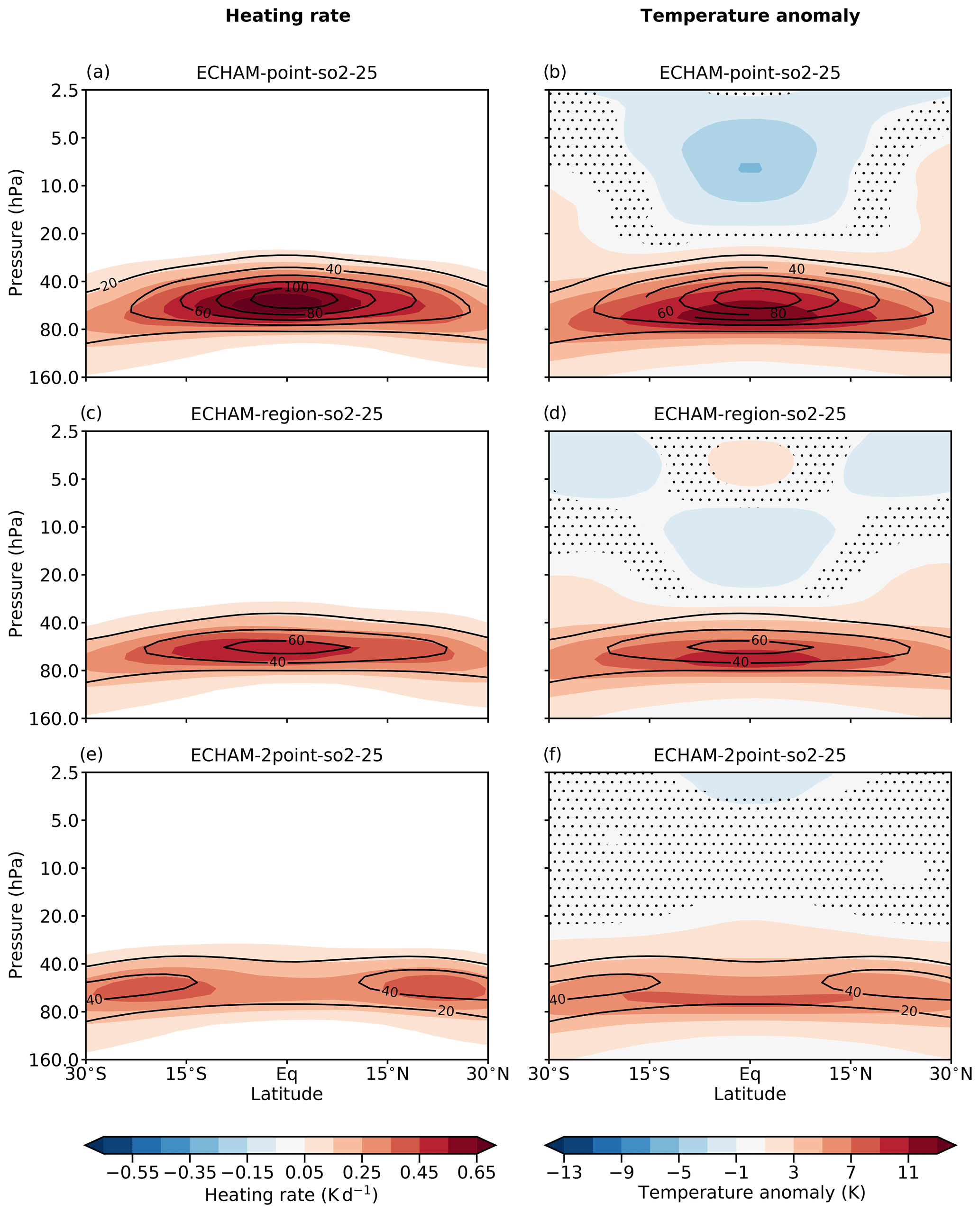
Figure 2Latitude–height cross section of the zonal mean net aerosol heating rate (a, c, e) and of the anomaly of the zonal mean temperature (b, d, f) for the ECHAM simulations of point-so2-25 (a, b), region-so2-25 (c, d), and 2point-so2-25 (e, f). Stippling indicates areas where the temperature anomalies are not significant at the 95 % level in Student's t test. Black contour lines indicate the anomaly of the zonal mean sulfate mass mixing ratio in intervals of 20 µg(S) kg−1.
This aerosol-induced heating results in a significant positive temperature anomaly centered at the Equator (Fig. 2b, d, f). Following the meridional structure of the net aerosol heating rates, the lower-stratospheric temperature anomaly has a clear equatorial peak for the point injection and its poleward gradients are sharp (Fig. 2b). For the region injection, the lower-stratospheric temperature anomaly still peaks at the Equator but with a smaller absolute magnitude, leading to a smaller poleward gradient (Fig. 2d). For the 2point injection, the temperature anomaly is meridionally nearly uniform between 15∘ N and 15∘ S (Fig. 2f).
The warming of the lower stratosphere is the primary perturbation induced by the sulfate aerosols, as indicated by the good agreement of the sulfate mass mixing ratio, the net aerosol heating rates, and the temperature anomalies. All changes in dynamics – including the QBO – are obviously induced by this initial warming in a second step.
Opposite to the lower-stratospheric warming, statistically significant negative temperature anomalies are located in the middle and upper tropical stratosphere for all three injection strategies (Fig. 2b, d, f). However, Fig. 2 clearly shows that this cooling is not induced by the radiative effects of the aerosols, as it is located well above the aerosol layer and does not match with the net aerosol heating rates. Consequently, these negative temperature anomalies have been induced dynamically due to an increased tropical upwelling (see Aquila et al., 2014). Therefore, they cannot be seen as a root cause of any change in the QBO.
3.1.2 Modification of the residual circulation
Following Aquila et al. (2014), an increase of the tropical upwelling in the rising branch of the BDC due to the aerosol-induced warming is the main reason for the modification of the QBO. Commonly, the BDC is treated in the so-called transformed Eulerian mean (TEM) framework as outlined by Andrews et al. (1987), in which it is represented by the residual mean circulation. The residual mean circulation itself may be described by the residual meridional and vertical velocities and , respectively, or by its mass stream function χ. For equatorial point injections of SO2, Aquila et al. (2014) showed that an aerosol-induced increase of is associated with a stronger residual vertical advection of zonal momentum (). A stronger in the tropical stratosphere weakens the downwelling of the QBO phases, which leads to a prolongation of the QBO period.
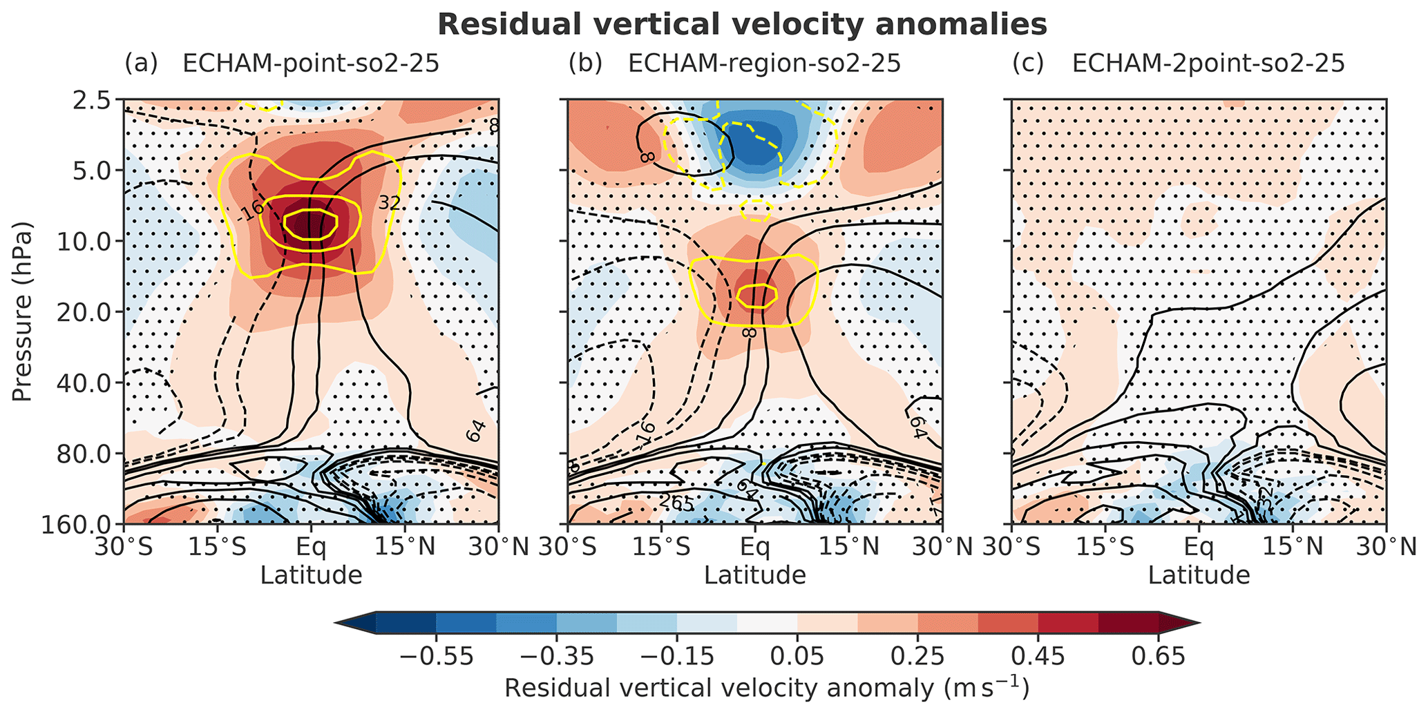
Figure 3Latitude–height cross section of the anomaly of the zonal mean residual vertical velocity for the ECHAM simulations of point-so2-25 (a), region-so2-25 (b), and 2point-so2-25 (c). Stippling indicates areas where anomalies are not significant at the 95 % level in Student's t test. Black contour lines show the anomaly of the zonal mean residual mass stream function χ in kilogram per second (kg s−1). The thin solid contours indicate a clockwise circulation anomaly, and the dashed contours indicate a counterclockwise circulation anomaly. The contour interval is logarithmic starting at 8 and −8 kg s−1 for the clockwise and counterclockwise anomalies, respectively, while the 0 kg s−1 contour is omitted. Yellow contour lines denote the residual vertical advection of zonal momentum with a contour interval of 0.3 , starting at 0.15 and −0.15 . The solid lines indicate a positive anomaly, the dashed lines indicate a negative anomaly, and the 0 contour is omitted.
Our simulations confirm that increases statistically significantly within the tropics for point-so2-25 and region-so2-25 and that this increase results in a stronger in the upper tropical stratosphere (Fig. 3a, b). Thereby, the anomalies are slightly stronger for point-so2-25 than for region-so2-25 due to the stronger aerosol-induced stratospheric warming. The maximum anomalies of are located at the altitudes of strongest easterly shear (see Fig. 1e, h). This indicates that the increase of the tropical upwelling helps to maintain the permanent westerlies against the downwelling easterlies aloft. For 2point-so2-25, and do not show a statistically significant increase throughout the whole tropical stratosphere (i.e., between 15∘ N and 15∘ S) (Fig. 3c). The zonal mean residual circulation as a whole is also only weakly modified in the tropical stratosphere. This is in accordance with our observation that the amplitude and the periodicity of the QBO basically remain unchanged for 2point-so2-25 (Fig. 1k).
The reason for the increase of is the aerosol-induced stratospheric temperature anomaly, which alters the characteristics of the zonal jets in the extratropical stratosphere. Thereby, the conditions for the vertical propagation of planetary waves in this region change. As a consequence, the extratropical wave driving of the residual mean circulation increases, which ultimately speeds up the whole BDC. This mechanism has been investigated by Tilmes et al. (2018) for SAM simulations and was also recognized in simulations of a tropical volcanic eruption by Bittner et al. (2016).
In the upper stratosphere (i.e., between 20 and 3 hPa in point-so2-25 and between 25 and 8 hPa in region-so2-25), this increase of is superimposed by changes in the secondary meridional circulation (SMC) of the modified QBO itself. During a permanent QBO westerly phase, the SMC would also be permanently locked in its corresponding “westerly” phase, which acts to increase within the tropical stratosphere (Plumb and Bell, 1982). Our experiments indicate that a large fraction of the increase of in the upper tropical stratosphere (Fig. 3a, b) can be attributed to this “indirect” acceleration via the SMC, especially in the upper stratosphere. For example, in the experiment point-so2-5, the tropical increased by up to 100 % in the upper stratosphere (not shown). In contrast, in ECHAM simulations with permanent lower-stratospheric easterlies instead of a QBO, Niemeier et al. (2011) obtained an increase of the tropical of only 5 % to 10 % for an equatorial point injection of SO2 with an injection rate of 4 Tg(S) yr−1. Therefore, one has to be cautious when interpreting the strong positive anomalies of observed in the upper stratosphere in point-so2-25 and region-so2-25 as the primary cause for the disruption of the QBO since they are – at least partly – rather its consequence.
Within the TEM framework, the characteristics of the general acceleration of the BDC can be further directly linked to the tropical confinement of the aerosol-induced temperature anomaly, as shown by Dunkerton (1983) in a study on the effect of the 1963 eruption of Mt. Agung on the QBO. Following the equation of the residual mean meridional streamfunction (Plumb and Bell, 1982), only a tropically confined heating modifies the BDC, whereas a meridionally uniform heating has no effect. This explains why the residual tropical upwelling increases in point-so-25 and region-so2-25 but not in 2point-so2-25: while in point-so2-25 and region-so2-25 the aerosol heating has an equatorial peak and decreases rather sharply towards the extratropics, in 2point-so2-25 it is meridionally nearly uniform within the tropics (see Sect. 3.1.1).
Consequently, it is ultimately the meridional shape of the aerosol-induced lower-stratospheric temperature anomaly or – simply spoken – the degree of tropical confinement of the artificial sulfate aerosols that determines the QBO response to artificial sulfate injections.
3.1.3 Modification of thermal wind balance
Besides the increase of the tropical upwelling in the rising branch of BDC, Aquila et al. (2014) also attributed the observed changes in the QBO to a modification of thermal wind balance. Thermal wind balance is an atmospheric state equation, which links the zonal mean meridional temperature gradient to the zonal mean vertical wind shear . It is defined as
for an equatorial β plane (Holton, 2004). Assuming equatorial symmetry of the zonal mean temperature field, one can set K km−1 at the Equator and apply the rule of L'Hospital (Holton, 2004):
Within Eqs. (1) and (2), R denotes the gas constant for dry air, H denotes the scale height, and β denotes the meridional gradient of the Coriolis parameter at the Equator. denotes the meridional curvature of the zonal mean temperature.
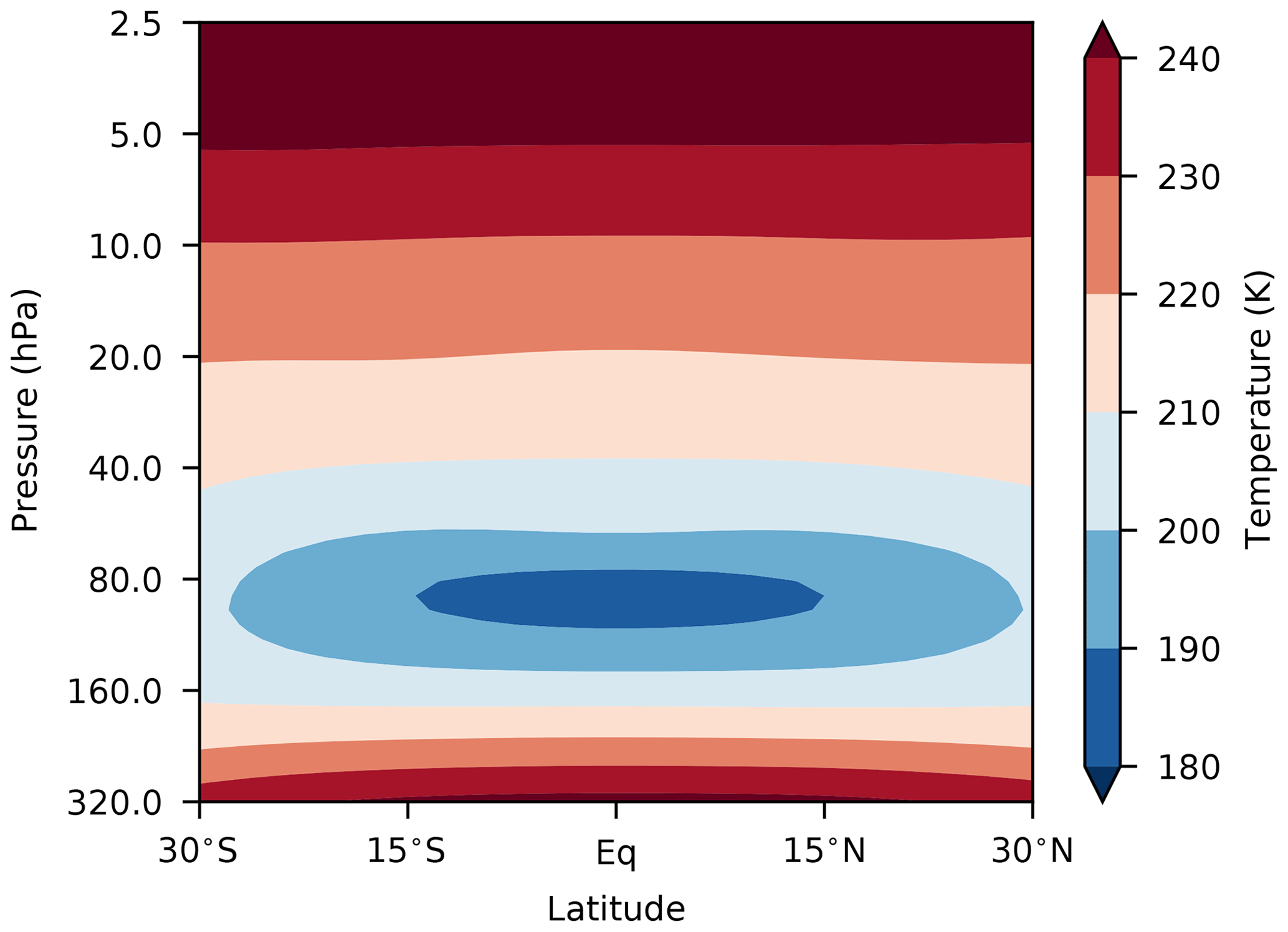
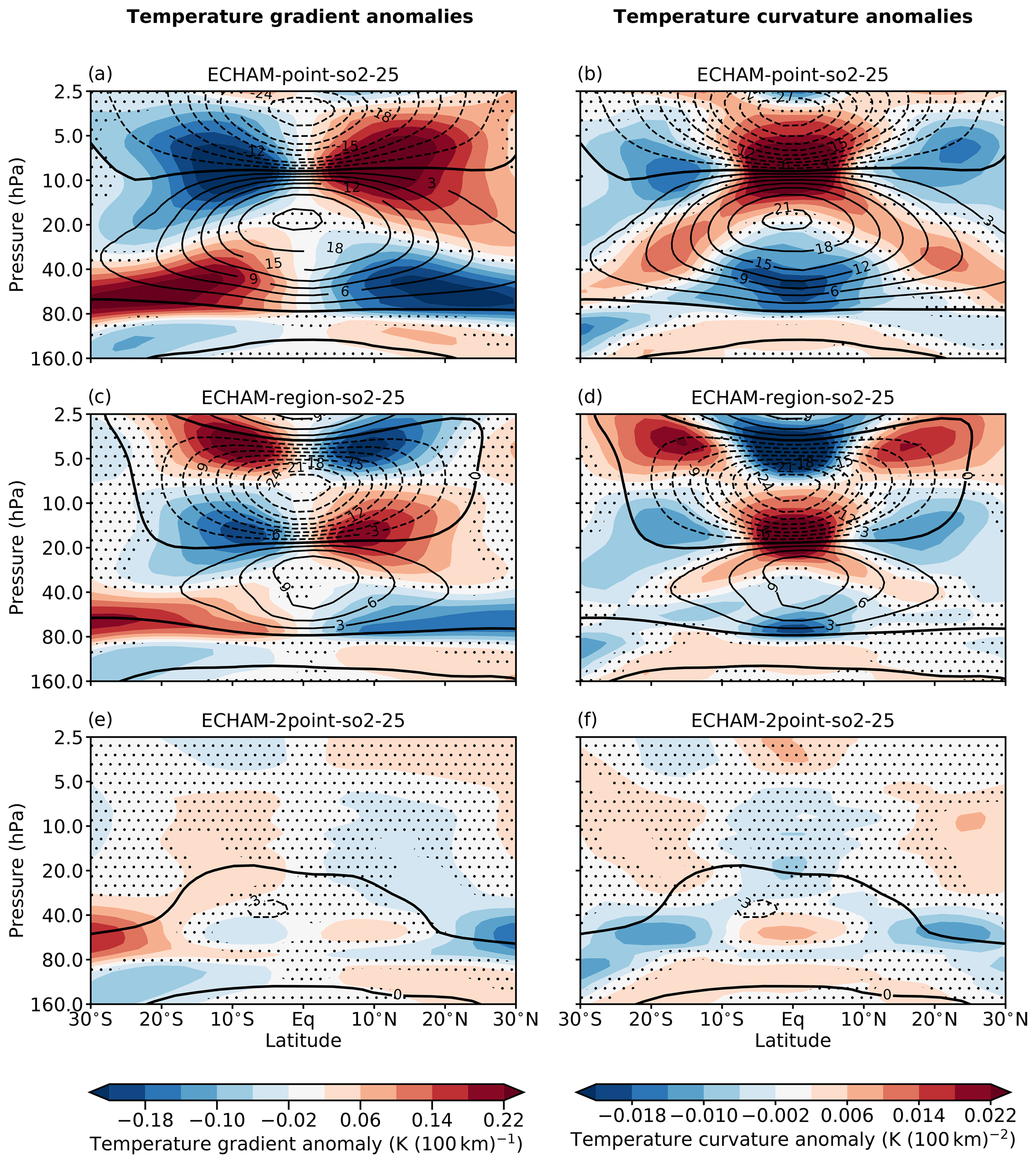
Figure 5Latitude–height cross section of the anomaly of the meridional zonal mean temperature gradient (a, c, e) and of the anomaly of the meridional zonal mean temperature curvature (b, d, f) for the ECHAM simulations of point-so2-25 (a, b), region-so2-25 (c, d), and 2point-so2-25 (e, f). Stippling indicates areas where anomalies are not significant at the 95 % level in Student's t test. Black contour lines indicate the anomaly of the zonal mean zonal wind speed in intervals of 3 m s−1, with the thick black line denoting m s−1. Solid lines denote a westerly anomaly; dashed lines denote an easterly anomaly.

Figure 6Vertical profile of the 5∘ N to 5∘ S mean temperature anomaly for the 5 and 25 Tg(S) yr−1 injections simulated with ECHAM. The horizontal grey bar marks the injection layer. The vertical dashed–dotted line marks a temperature anomaly of 0 K.
However, despite the fact that QBO changes due to artificial sulfur injections are frequently interpreted as a consequence of an increased residual tropical upwelling and a modification of thermal wind balance, one can not see both as two separate processes. In contrast, the acceleration of the BDC discussed in Sect. 3.1.2 is rather the mechanism by which thermal wind balance is re-established for the aerosol-induced lower-stratospheric temperature anomaly (Holton, 2004). While the differences in the increase of directly explain the different QBO responses to different injection strategies in a straightforward manner (see Sect. 3.1.2), in this section we show that the differences in the QBO response can be also linked directly to the meridional shape of the aerosol-induced lower-stratospheric temperature anomaly via thermal wind balance.
As discussed in Sect. 3.1.1, an equatorial point injection results in a significant positive temperature anomaly centered at the Equator (Fig. 2b). In the climatological mean – without artificial sulfur injections and represented by contr-000 – the lower tropical stratosphere is much colder than the lower midlatitudinal stratosphere (Fig. 4), leading to a poleward that is positive. The aerosol-induced warming abates the poleward (Fig. 5 a) within the lower tropical stratosphere between 40 and 80 hPa, which is accompanied by a significant negative anomaly of centered at the Equator (Fig. 5b). Following Eq. (2), a negative anomaly of results in stronger westerly shear. Consequently, a strong westerly anomaly of the zonal mean zonal wind is located on top of the injection layer in order to maintain thermal wind balance (Fig. 5b). This results in the observed constant westerly QBO phase (Fig. 1b).
For region-so2-25, the QBO was also found to be locked in a permanent westerly phase, but the vertical extent as well as the strength of the westerlies is weaker than for point-so2-25, which is in agreement with the results of Niemeier and Schmidt (2017). The reason for the weaker westerlies is the meridionally more uniform temperature anomaly within the lower tropical stratosphere (Fig. 2d). Therefore, the strongest modifications of in the lower stratosphere are located poleward of approximately 20∘ N and 20∘ S, while its modification close to the Equator is relatively small (Fig. 5c). Accordingly, also the negative anomaly of and – following thermal wind balance (Eq. 2) – the induced anomaly of westerly shear is weaker near the Equator compared to point-so2-25 (Fig. 5d). Consequently, the lower-stratospheric westerly anomaly of is weaker for region-so2-25 than for point-so2-25.
For 2point-so2-25, the QBO was not found to be modified significantly, and it basically preserved its natural periodicity (Fig. 1k). Due to the extratropical injection locations, the highest sulfate concentrations are located at approximately 20∘ N and 20∘ S and so is the associated heating (Fig. 2e). Therefore, the lower-stratospheric temperature anomaly is meridionally nearly uniform between approximately 15∘ N and 15∘ S (Fig. 2 f). Consequently, and are only very weakly modified between 40 and 80 hPa and between approximately 15∘ S and 15∘ N (Fig. 5e, f), and these anomalies are hardly statistically significant. Following thermal wind balance, this implies that zonal wind anomalies in the lower stratosphere are small as well (Fig. 5e, f), which is in accordance with the QBO in principle remaining in its natural shape.
As discussed in Sect. 3.1.1, the negative temperature anomalies above approximately 20 hPa have been induced dynamically due to an increased tropical upwelling and negative temperature advection (see Aquila et al., 2014). While the corresponding anomalies of and above 20 hPa are of course still in thermal wind balance with the upper-stratospheric wind field (Fig. 5), it is important to mention that this agreement does not imply causality in the way that these upper-stratospheric temperature anomalies have caused the lower-stratospheric westerly anomaly and QBO modification.
Our results clearly show that differences in the QBO response with respect to our three tested injection strategies are linked to differences in the meridional structure of the aerosol-induced temperature anomaly. Therefore, the absolute strength of the aerosol-induced lower-stratospheric temperature anomaly does not permit a statement about the strength of the QBO modification when comparing different injection strategies. For instance, the tropical (i.e., 5∘ N to 5∘ S) mean temperature anomaly within the injection layer is more than twice as high in 2point-so2-25 than in point-so2-5 (Fig. 6). However, the QBO is heavily perturbed in point-so2-5, while for 2point-so2-25 it remains nearly unchanged (Fig. 1d, k). This comparison shows that within
which is often used as an approximation of thermal wind balance for QBO variations centered at the Equator (Baldwin et al., 2001); the scaling factor L depends on the injection strategy. Therefore, Eq. (3) cannot be used when comparing the QBO response to different injection strategies.
Since it is the degree of tropical confinement of the artificial sulfate aerosols that is ultimately decisive for the observed QBO response also when explaining the observed QBO changes solely as the consequence of an increased residual tropical upwelling, we will use thermal wind balance in our argumentation throughout this study as it directly links the observed QBO changes to the observed aerosol-induced temperature anomalies.
3.2 Impact of injection rate
For the point and the region injection strategies, the QBO was found to be impacted much less in our experiments with an injection rate of 5 Tg(S) yr−1 than in those with an injection rate of 25 Tg(S) yr−1, and it basically maintained its oscillating behavior (Fig. 1d, g). This is explained by the clearly lower tropical sulfate burden, which results from the lower injection rate. The sulfate burden determines the strength of the lower-stratospheric heating by absorption of OTLR and NIRR. Accordingly, the tropical mean temperature anomalies are clearly weaker in our experiments with an injection rate of 5 Tg(S) yr−1 than in those ones with an injection rate of 25 Tg(S) yr−1 (Fig. 6). In contrast, the temperature anomaly in the extratropical stratosphere is rather independent of the injection rate for all injection strategies (not shown), since absorptive heating is generally weak in this region due to low values of OTLR and NIRR. Therefore, changes much less for a lower injection rate. The tropical mean anomalies of in and slightly above the injection layer are clearly smaller and vertically less extended for an injection rate of 5 Tg(S) yr−1 compared to 25 Tg(S) yr−1 (Fig. 7a). Following Eq. (2), this results in significantly smaller anomalies of the tropical mean zonal wind within the lower stratosphere (Fig. 7b). For the point and the region injection strategies, the strength of the westerly anomaly is reduced by a factor of ∼10 when reducing the injection rate from 25 to 5 Tg(S) yr−1, and consequently the QBO is not locked in a permanent westerly phase (Fig. 1d, g). For the 2point injection strategy, the tropical mean anomaly of is small for both tested injection rates (Fig. 7a). Accordingly, the QBO was found to be not modified significantly for either tested injection rates when applying the 2point injection strategy.
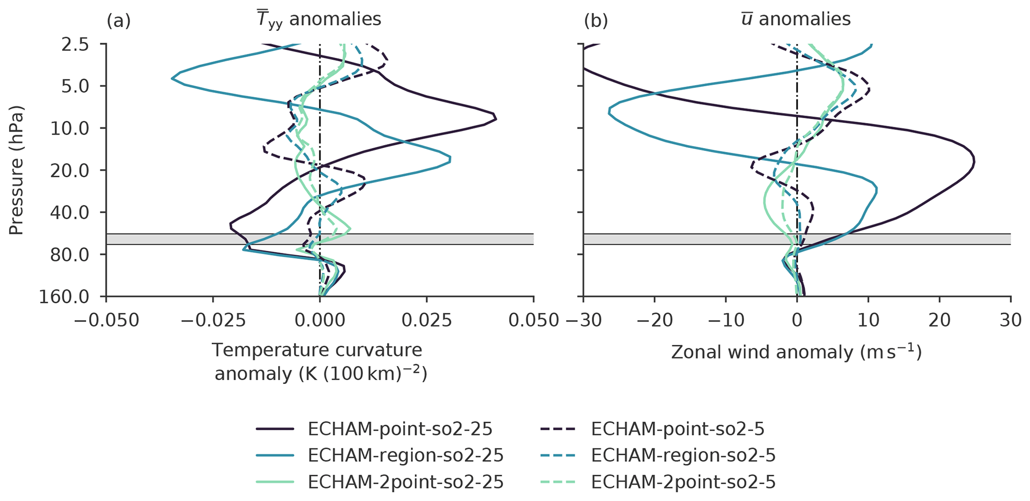
Figure 7Vertical profile of the 5∘ N to 5∘ S mean anomaly of the temperature curvature (a) and the tropical mean anomaly of the zonal wind (b) for the ECHAM simulations of a SO2 injection with an injection rate of 5 Tg(S) yr−1 (dashed) and 25 Tg(S) yr−1 (solid). The horizontal grey bar marks the injection layer. The vertical dashed–dotted line marks an anomaly of 0 K (100 km)−2 (a) and 0 m s−1 (b).
3.3 Impact of injection species
For all three tested injection strategies, the response of the QBO is in principle independent of the injection species – SO2 or AM−SO4 – in our experiments with an injection rate of 25 Tg(S) yr−1 (Fig. 1). This is reasonable, since the meridional distribution of the artificial sulfate aerosols, which can be seen as a proxy for the strength of the lower-stratospheric temperature anomaly, does in principle exhibit the same shape for both tested injection species except for different absolute values (Fig. 8). We showed that the modification of the QBO depends clearly on the meridional structure of the stratospheric temperature anomaly and is rather independent of its absolute value (Sect. 3.1.3).
However, for the point and region injection strategies, the modification of the QBO was found to be slightly stronger with respect to the strength and the vertical extent of the lower-stratospheric westerlies when injecting AM−SO4 instead of SO2 based on our experiments with an injection rate of 25 Tg(S) yr−1 (Fig. 1). This is a consequence of the in general higher sulfate burden, which results from an injection of AM−SO4 compared to an injection of SO2. As described in Sect. 3.2, the accompanied stronger warming of the lower tropical stratosphere relative to the midlatitude one results in a stronger modification of (Fig. 9a). However, the difference in the anomaly between both injection species is statistically significant at the 95 % level in Student's t test only for the point injections. This causes a stronger QBO westerly phase for an injection of AM−SO4 compared to an injection of SO2 as indicated by the anomalies of (Fig. 9b). The difference in the anomaly between both injection species is statistically significant at the 95 % level in Student's t test for both the point and the region injections. For the 2point injections of 25 Tg(S) yr−1, an injection of AM−SO4 instead of SO2 causes the opposite effect as it slightly weakens the positive anomaly of and within the tropics (Fig. 9).
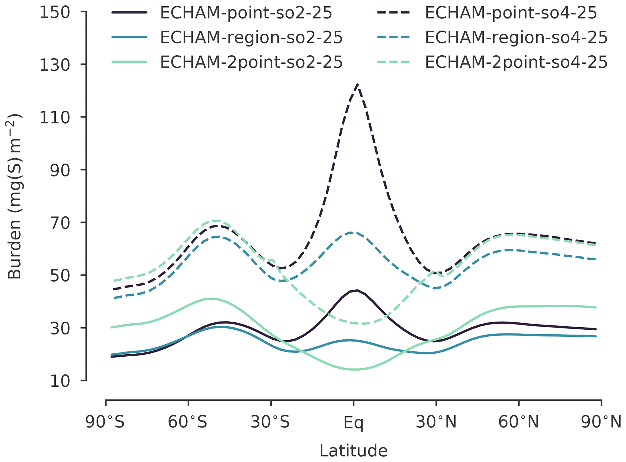
Figure 8Zonal mean artificial sulfate burden for the ECHAM simulations of the SO2 injections (dashed lines) and the H2SO4 injections (solid lines) with an injection rate of 25 Tg(S) yr−1 as a function of latitude.
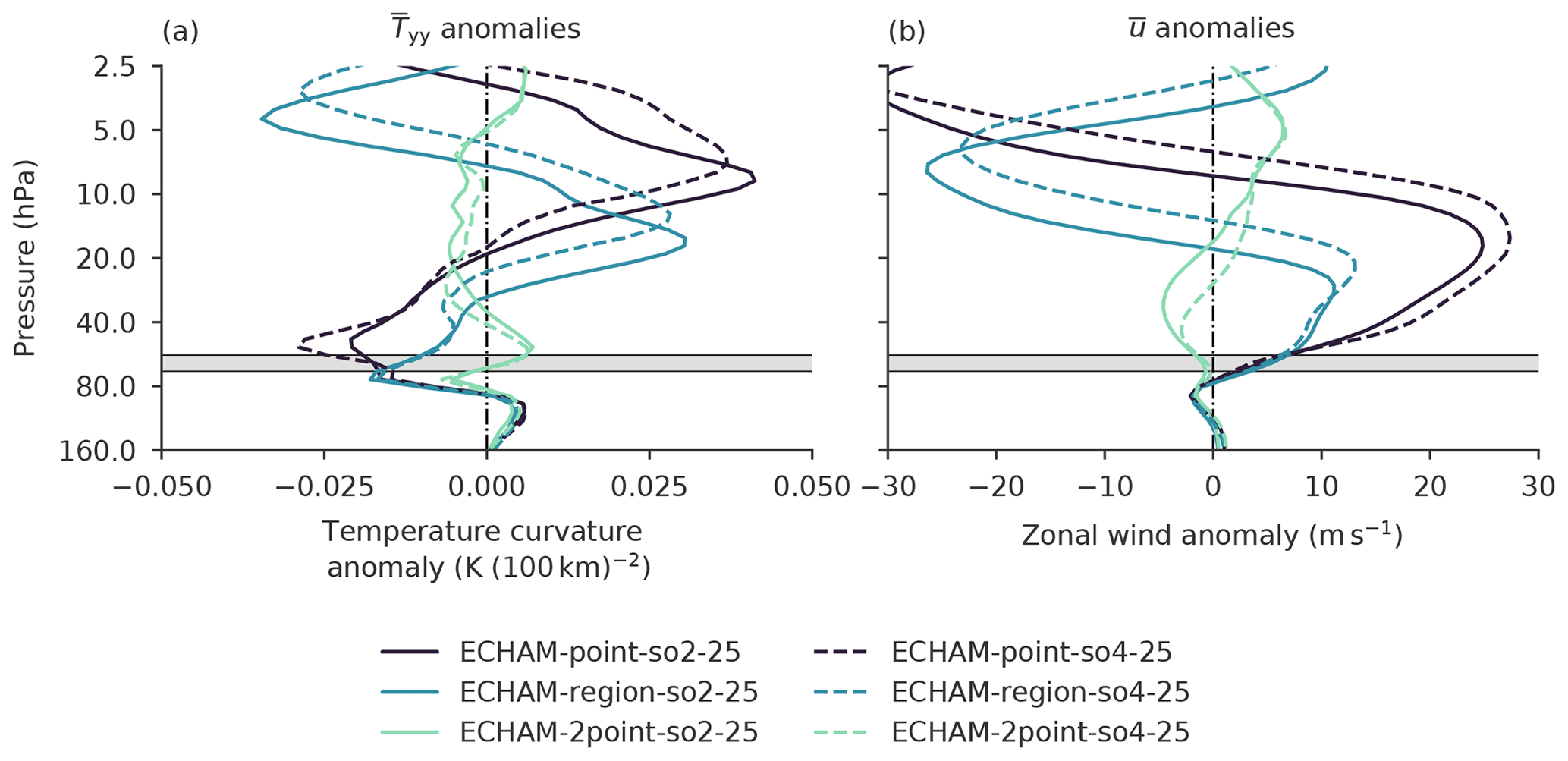
Figure 9Vertical profile of the 5∘ N to 5∘ S mean anomaly of the temperature curvature (a) and the tropical mean anomaly of the zonal wind (b) for the ECHAM simulations of injections with an injection rate of 25 Tg(S) yr−1. The horizontal grey bar marks the injection layer. The vertical dashed–dotted line marks an anomaly of 0 K (100 km)−2 (a) and 0 m s−1 (b).
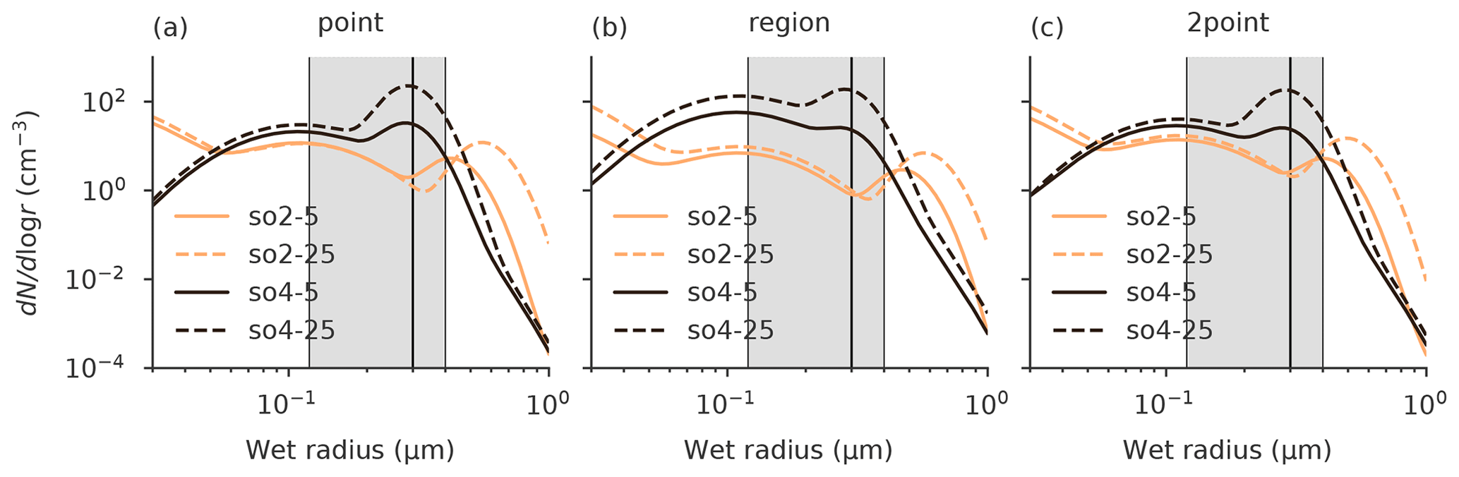
Figure 10Global mean aerosol size distributions focusing on AM−SO4 and coarse mode sulfate (CM−SO4) particles at 62 hPa, which is the central level of the injection layer, for the ECHAM simulations of the point injections (a), the region injections (b), and the 2point injections (c). The grey bar marks the size range in which the backscattering efficiency of an aerosol particle with a given wet radius is at least 70 % (i.e., 0.12–0.40 µm) of its maximum value, which is achieved for aerosols with a wet radius of 0.30 µm and marked by a thick solid black line (Dykema et al., 2016).
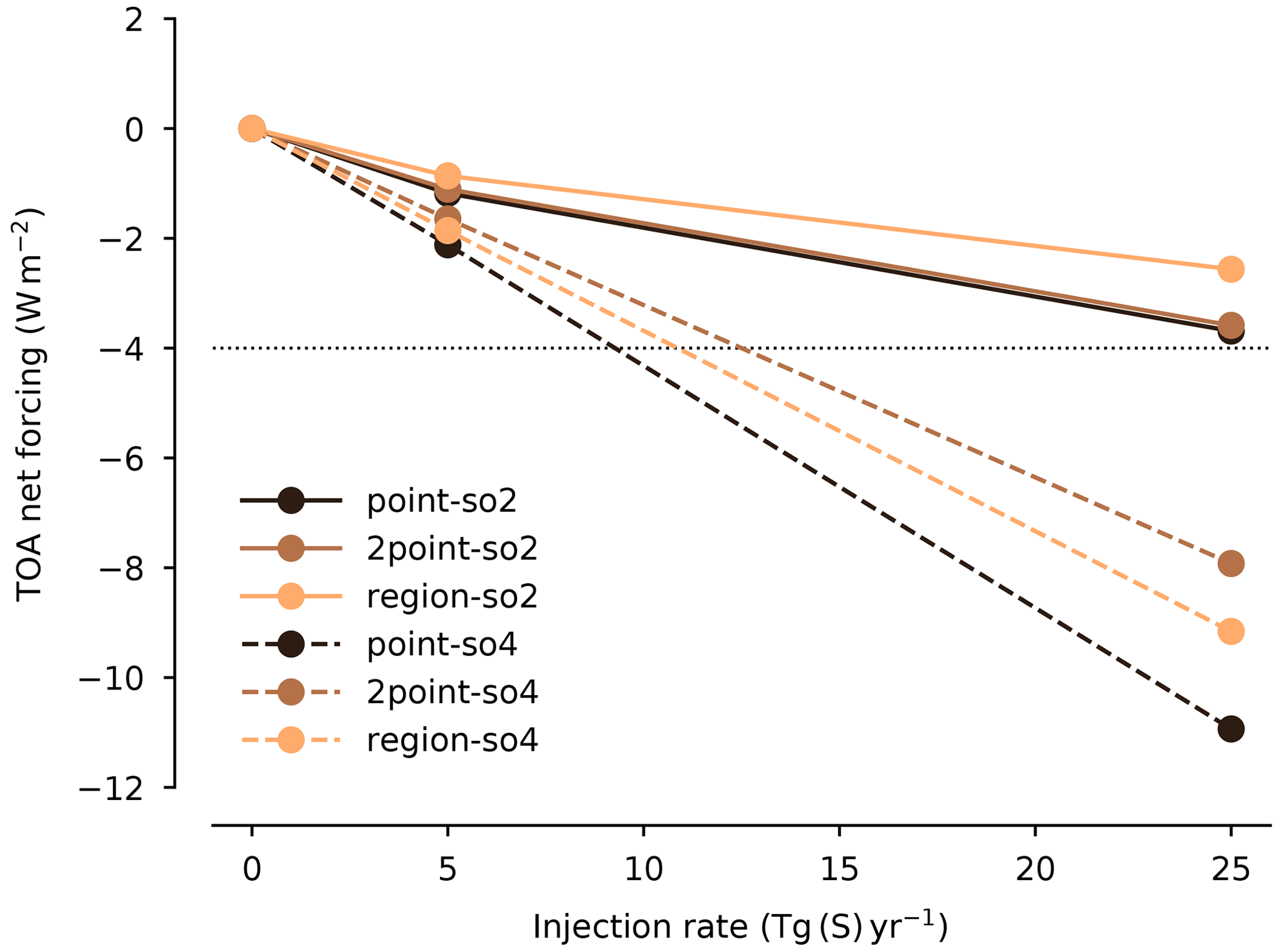
Figure 11Global mean top-of-atmosphere (TOA) all-sky net RF exerted by artificial sulfate aerosols as a function of injection rate. The dotted black line marks a RF of −4 W m−2.
The reason for the higher sulfate burden obtained for an injection of AM−SO4 compared to an injection of SO2 is differences in microphysical processes. Due to weaker coagulation and condensation, the sulfate particles stay on average smaller for an injection of AM−SO4 than for an injection of SO2 for all tested injection scenarios (Fig. 10). This reduces their sedimentation and enhances their stratospheric lifetime, which explains the larger sulfate burden. Additionally, smaller sulfate particles have a higher backscattering efficiency (Fig. 10). Therefore, the RF efficiency (RF per injected amount of sulfur) is also significantly higher for an injection of AM−SO4 than for an injection of SO2 (Fig. 11). The required injection rate to achieve a given RF is consequently clearly smaller for an injection of AM−SO4 compared to an injection of SO2. For example, to counteract a RF of 4.0 W m−2 as proposed in the GeoMIP6 experiment G6sulfur (Kravitz et al., 2015), an injection of SO2 would require injection rates of more than 25 Tg(S) yr−1, while an injection rate of about 10 to 12.5 Tg(S) yr−1 would be sufficient for an injection of AM−SO4, depending on the injection strategy (Fig. 11). The higher RF efficiency of an injection of H2SO4 should therefore be considered when comparing the QBO response between both tested injection species.
Both models simulate a reasonable QBO in the control simulation (Fig. 12a, b). With roughly 32 months the simulated QBO period of ECHAM is slightly longer than the one simulated in CESM, which is approximately 27 months. Both compare well to the observed period of 28 months on average (Naujokat, 1986). The simulated QBO winds, especially the QBO westerlies, are substantially stronger in ECHAM than in CESM at altitudes above 40 hPa. Accordingly, the QBO easterly phases are longer and relatively stronger in CESM at altitudes below 30 hPa. These general differences of the simulated QBO have to be considered when comparing the QBO response to different SAM scenarios in both models.
In the following two sections, the QBO response to the 2point and region injections will be compared for ECHAM and CESM based on the injection of AM−SO4 only. For an injection of SO2 instead of AM−SO4, the observed characteristics of the QBO remain basically the same in both models (See Sect. 3.3) and corresponding plots for an injection of SO2 can be found in the Supplement. A comparison of the QBO response to the point injection strategy is not possible, since the point injection is not part of the accumH2SO4 experimental protocol and was, therefore, not performed by CESM.
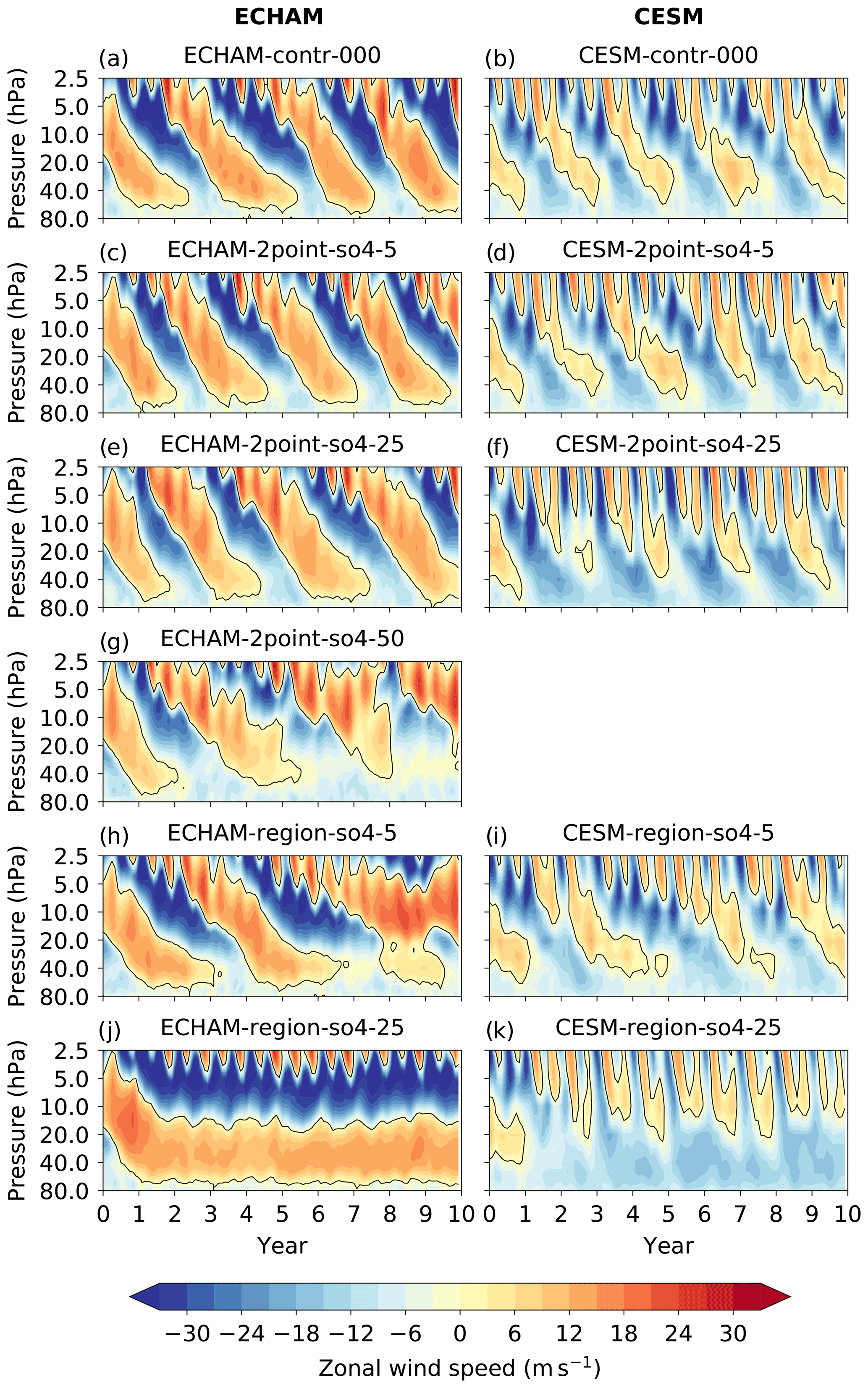
Figure 12Time–height cross sections of the 5∘ N to 5∘ S mean zonal wind in the stratosphere over the simulation period of 10 years for the AM−SO4 injection scenarios in ECHAM (left column) and CESM (right column). The first row shows the control simulation, the second row shows the 2point injections of 5 Tg(S) yr−1, the third row shows the 2point injections of 25 Tg(S) yr−1, the fifth row shows the region injections of 5 Tg(S) yr−1, and the sixth row shows the region injections of 25 Tg(S) yr−1. The 2point injection of 50 Tg(S) yr−1 was only performed with ECHAM and is shown in the fourth row. The solid black line marks a tropical mean zonal wind speed of 0 m s−1.
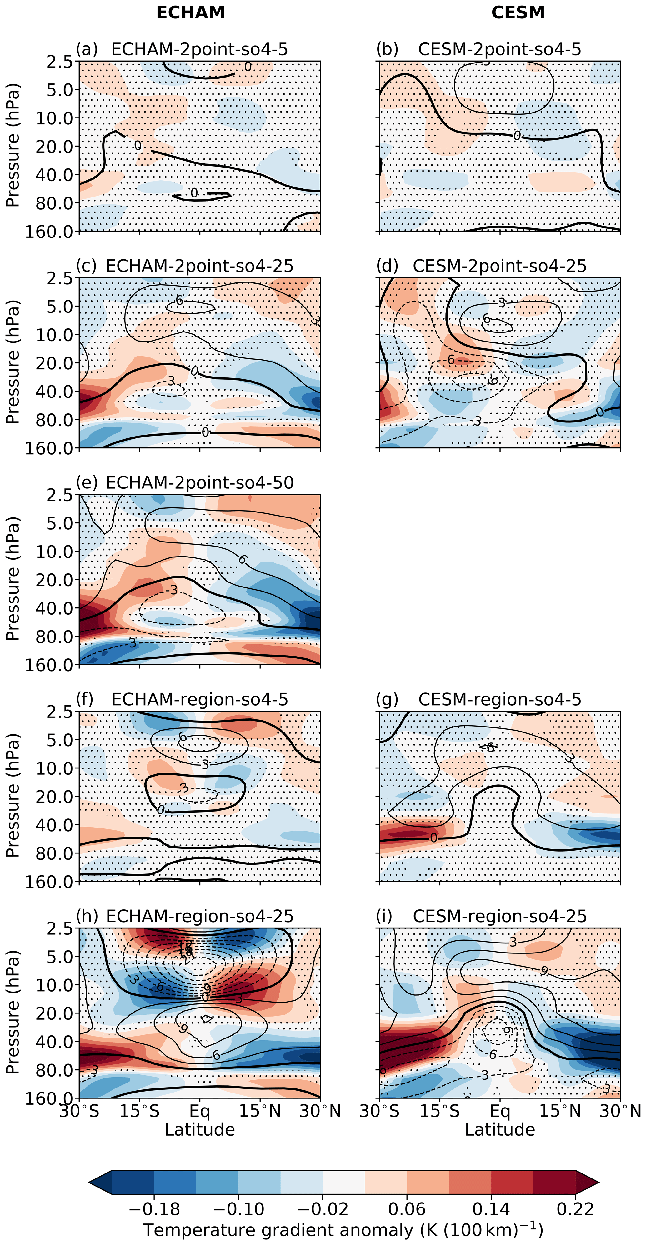
Figure 13Latitude–height cross sections of the anomaly of the meridional zonal mean temperature gradient for the AM−SO4 injection scenarios in ECHAM (left column) and in CESM (right column). Stippling indicates areas where anomalies are not significant at the 95 % level in Student's t test. Black contour lines indicate the anomaly of the zonal mean zonal wind speed in intervals of 3 m s−1, with the thick black line denoting m s−1. Solid lines denote a westerly anomaly, while dashed lines denote an easterly anomaly. The first row shows the 2point injections of 5 Tg(S) yr−1, the second row shows the 2point injections of 25 Tg(S) yr−1, the fourth row shows the region injections of 5 Tg(S) yr−1, and the fifth row shows the region injections of 25 Tg(S) yr−1. The 2point injection of 50 Tg(S) yr−1 was only performed with ECHAM and is shown in the third row.
4.1 2point injection strategy
For the 2point injections of AM−SO4 simulated in ECHAM, the periodicity and strength of the QBO are basically not modified for the tested injection rates of 5 and 25 Tg(S) yr−1 (Fig. 12c, e). However, for an injection rate of 25 Tg(S) yr−1 a slight easterly anomaly of up to −3 m s−1 has been noticed at approximately 40 hPa and 5∘ S (Fig. 13 c), which is at the edge of extreme natural variability based on Student's t test. In CESM, the QBO is also not modified much relative to the control simulation for the 2point injections with an injection rate of 5 Tg(S) yr−1 (Fig. 12d). For an injection rate of 25 Tg(S) yr−1, the QBO basically maintains its oscillating behavior in CESM as well (Fig. 12f) but with clearly stronger easterlies and weaker westerlies at altitudes below 20 hPa compared to the control simulation.
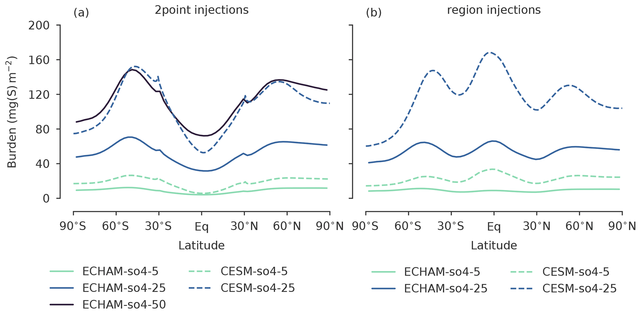
Figure 14Zonal mean artificial sulfate burden for the 2point injections (a) and the region injections (b) of AM−SO4 as a function of latitude. Solid lines indicate the ECHAM simulations; dashed lines indicate the CESM simulations. The artificial sulfate burden can be used as a very basic proxy for the amount of heating due to absorption of OTLR and NIRR.
Nevertheless, the QBO responds qualitatively similar to a 2point injection of AM−SO4 in both models, which is clearly shown by Fig. 12c–f. The spatial structure of the anomalies, indicated by the contour lines in Fig. 13, does in general agree for both models and both tested injection rates (Fig. 13a–d). For an injection rate of 25 Tg(S) yr−1, it shows a lower-stratospheric easterly anomaly centered at approximately 40 hPa and 5∘ S and an upper-stratospheric westerly anomaly, which further extends into the Northern Hemisphere. The anomaly of also shows basically the same spatial structure in both models as the usually positive poleward between approximately 80 and 40 hPa strengthens statistically significantly. For a given injection rate, this strengthening – located approximately between 80 and 40 hPa and between 20∘ S and 20∘ N – is clearly stronger and vertically more extended in CESM (Fig. 13c, d), which explains the stronger easterly anomaly observed in CESM as a consequence of thermal wind balance (Eq. 1). Figure 14a demonstrates the reason for the more significant strengthening of the poleward in CESM. In accordance with Niemeier et al. (2020), the sulfate burden for a given injection rate is substantially larger in CESM than in ECHAM, which is predominantly due to a stronger . Given the characteristic meridional distribution of sulfate particles for a 2point injection, this results in a higher sulfate burden in the subtropical stratosphere relative to the tropical one in CESM (Fig. 14a). This is the reason for the stronger modification of for a given injection rate in CESM compared to ECHAM.
Following Niemeier et al. (2020), we therefore performed an ECHAM simulation of a 2point injection which results in approximately the same global mean sulfate burden and the same meridional distribution of sulfate particles like the CESM simulation of a 2point injection with an injection rate of 25 Tg(S) yr−1. This is the case for an injection of 50 Tg(S) yr−1 in ECHAM (Fig. 14a). As visible in Figure 12g, the QBO easterly phases are substantially prolonged also in ECHAM for injections with an injection rate of 50 Tg(S) yr−1. In this simulation, the QBO westerlies in the lower stratosphere at altitudes below 20 hPa are clearly weaker than in the control simulation (Fig. 12g). Overall, the spatiotemporal structure of the QBO jets agrees reasonably well between the CESM simulation with an injection rate of 25 Tg(S) yr−1 and the ECHAM simulation of 50 Tg(S) yr−1, given the general differences of the simulated QBO of both models. Additionally, also the anomalies of and agree reasonably well with each other (Fig. 13d, e). This indicates that the QBO does in principle respond similarly to a 2point injection of AM−SO4 in both models but that this response is more sensitive to an increase of the injection rate in CESM than in ECHAM, which is in agreement with Niemeier et al. (2020). Nevertheless, the QBO response is still stronger in CESM than in ECHAM, and the reason for this has not been conclusively determined.
4.2 Region injection strategy
In contrast to the 2point injections, the response of the QBO to a region injection of AM−SO4 is fundamentally different in ECHAM and CESM. For an injection rate of 5 Tg(S) yr−1, the QBO slows down in both models with lower-stratospheric winds being predominantly westerly in ECHAM, while being more easterly in CESM (Fig. 12h, i). For an injection rate of 25 Tg(S) yr−1, the lower-stratospheric QBO is locked in a permanent westerly phase in ECHAM, while it is locked in a permanent easterly phase in CESM (Fig. 12j, k). Accordingly, in ECHAM has a westerly anomaly of up to +12 m s−1 at the Equator at a pressure level of approximately 25 hPa, while in CESM it has an easterly anomaly of more than −10 m s−1 at the same location (Fig. 13h, i).
For ECHAM, the results are explained by the weakening of the usually positive poleward due to the aerosol-induced warming of the lower tropical stratosphere, which induces additional westerly shear within the injection layer centered at 60 hPa (see Sect. 3.1.3). Figure 13 h shows that the anomalies of reach far into the tropics at altitudes between 20 and 80 hPa for the ECHAM simulation of region-so4-25. In contrast, the anomalies within the same height range are only weak between 10∘ S and 10∘ N in the corresponding CESM simulation (Fig. 13i). They even slightly change sign locally. This indicates that the warming of the lower tropical stratosphere relative to the midlatitude one is clearly weaker in CESM than in ECHAM. The resulting aerosol-induced temperature anomaly is meridionally more uniform in CESM, which corresponds to the observed easterly anomalies of in CESM.
However, Fig. 14b shows that the observed differences in between both models cannot be explained by differences in the meridional distribution of sulfate. For both models, the meridional distribution of sulfate basically exhibits the same shape with a distinct equatorial peak and two additional local maxima located approximately at 50∘ S and 50∘ N. Based on this, we would have expected basically the same QBO response for both models.
4.3 Impact of ozone depletion on the QBO response
We assume that the significant difference in the QBO response to a region injection of AM−SO4 between CESM and ECHAM is explained at least partly by the interactive treatment of ozone in CESM. Figure 15 shows that in the CESM simulations the artificial injections of AM−SO4 lead to a strong depletion of ozone at altitudes between 20 and 40 hPa. Thereby, the strength and the location of the negative ozone anomalies closely correspond to the spatial distribution of the sulfate aerosols as represented by the sulfate mass mixing ratio. For the region injections, this implies that the aerosol-induced lower-stratospheric heating by the absorption of OTLR and NIRR is at least partly compensated by a reduction of shortwave (SW) heating due to ozone depletion, especially within the tropics in between 15∘ S and 15∘ N. For example, the region injection of 25 Tg(S) yr−1 results in an ozone depletion of more than −1.5 ppm at the Equator at an altitude of approximately 25 hPa compared to the control simulation (Fig. 15d). This corresponds to a change of about −30 %. Consequently, also the ozone-related SW heating at this altitude would be reduced by approximately 30 %. We argue that for the region injections this partial compensation of aerosol-induced heating by ozone-induced cooling is likely to contribute significantly to the observed different anomalies of in the lower tropical stratosphere between 40 and 80 hPa in CESM compared to ECHAM (Fig. 13f–i). Thereby, the aerosol-induced changes in the ozone concentration help to prevent the QBO from being locked in a permanent lower-stratospheric westerly phase like in ECHAM, which has no interactive ozone chemistry. Our theory is in agreement with ECHAM simulations of an equatorial point injection of SO2 using a prescribed ozone field, which was interactively calculated in corresponding CESM simulations. These ECHAM simulations resulted in a weaker westerly anomaly of the QBO winds than the ECHAM simulations of this study (Henning Franke and Ulrike Niemeier, personal communication, 2020).

Figure 15Latitude–height cross section of the ozone concentration anomaly for the simulations of an AM−SO4 injection in CESM. Stippling indicates regions where anomalies are not significant at the 95 % level in Student's t test. Contour lines indicate the zonal mean sulfate mass mixing ratio in microgram per kilogram (µg kg−1). The contour interval is logarithmic starting at 2 µg kg−1. The sulfate mass mixing ratio can be reasonably used as a proxy for the heating rate due to absorption of OTLR and NIRR.
However, based on our analysis we cannot fully explain why the QBO is locked in a strong permanent easterly phase in CESM. The lower-stratospheric ozone depletion and the upper-stratospheric ozone increase alone may only partly account for this substantial difference between both of our models. Most likely, differences in the SAM-induced changes of the resolved and parameterized wave forcing of the QBO may explain its different responses to SAM in both models. Additionally, differences in the GW parameterization of both models itself are likely to account to the observed differences, as they are tuned to represent the QBO realistically in the current climate but may react very differently to an external forcing like artificial sulfate aerosols.
For the 2point injections, changes in stratospheric ozone levels are mostly located outside the equatorial region (Fig. 15a, c). Therefore, tropical SW heating may not be altered significantly, which explains why for the 2point injections the response of the QBO as an equatorial system was found to be in principle the same for both models.
4.4 Characteristics of ozone depletion in CESM
The ozone changes observed in the CESM simulations are consistent with previous simulations with the older version of the same model (CESM1(WACCM); see, for instance, Tilmes et al., 2017, and Richter et al., 2017) and appear to be mostly independent from the type of injection, except for slight differences in the overall burden already discussed. The 2point simulations result in little changes in ozone concentration near the Equator, due to lower SO4 concentrations, while a decrease is observed in the subtropics and midlatitudes (Fig. 15a, c). This ozone decrease is mostly driven by the increase in the surface area density (SAD) produced by the aerosols that enhances the ozone destruction by halogens (such as HOCl) in the heterogeneous reaction (at T<200 K)
where ClONO2 is one of the main stratospheric reservoirs of inorganic chlorine (see Seinfeld and Pandis, 1998, Sect. 5.6). In the region simulations, on the other hand, the ozone changes turn out to be more similar to those observed in previous studies for equatorial point injections (Fig. 15b, d). This is due to the higher SO4 concentration in the tropical lower stratosphere, which also tends to extend in the middle stratosphere due to stronger upwelling. In this case, while the ozone reduction in the lower stratosphere can be attributed to the same heterogeneous chemistry mechanism described above, the ozone increase in the middle stratosphere can be explained by the predominance of the NOx cycle for the ozone budget at those altitude. The enhanced SAD results in a reduction in reacting nitrogen (N2O5, which is a catalyst for ozone destruction) due to the heterogeneous reaction
that, in turn, reduces the NOx-driven ozone loss cycle (Visioni et al., 2017b). The two effects combine, however, resulting in no changes in the tropical stratospheric ozone column. At higher latitudes, the similar SO4 distributions result in identical ozone changes in the ozone column. For more details on stratospheric ozone depletion we refer to Tilmes et al. (2018).
Within this study, we performed several simulations with the GCMs ECHAM and CESM to comprehensively compare the response of the QBO to different SAM setups with regard to the injection strategy, the injection rate, and the injection species. Thereby, we aimed at a deeper investigation of the reasons for structural differences in the QBO response to different SAM setups. We identified the following key characteristics of the QBO response to SAM:
-
The QBO response to SAM does fundamentally depend on the injection strategy. The injection rate and species rather act to scale the strength of this response.
-
We clearly identified the meridional structure of the aerosol-induced temperature anomaly within the lower tropical stratosphere instead of its absolute strength as the key parameter explaining the observed different responses of the QBO to our different injection setups.
-
For the equatorial point and for the region injections, the aerosol warming peaks more or less sharply at the Equator, causing a weakening of the poleward in the lower tropical stratosphere. This generates a westerly wind anomaly and eventually forces the QBO into a permanent westerly phase.
-
In contrast, is basically not modified in the tropics for the 2point injections due to a meridionally nearly uniform warming. Therefore, the QBO remains approximately in its natural state.
Obviously, linking the QBO response to artificial sulfur injections to the meridional shape of the aerosol-induced temperature anomaly offers us the possibility to explain the fundamentally different responses of the QBO to all of our three injection strategies simulated with ECHAM in a stringent manner. This is a clear advancement compared to earlier studies, e.g., Niemeier and Schmidt (2017) or Tilmes et al. (2018), which did not adequately discuss differences in the QBO response between different injection strategies. The dependency of the QBO modification on the meridional structure of the lower-stratospheric temperature anomaly via thermal wind balance may also be helpful to explain the significant acceleration of the QBO found by Richter et al. (2017) for extratropical single-point injections at 15∘ S, 15∘ N, 30∘ S, and 30∘ N, of which the causes were not finally determined.
Therewith, our results indicate that the modification of thermal wind balance in the lower tropical stratosphere between 40 and 80 hPa is a simple but sufficient framework to explain the simulated differences in the QBO modification for our three tested injection strategies as it directly links the zonal wind anomaly to the anomaly. Furthermore, we have shown that the different QBO responses to the different injection strategies correspond to the observed differences in the acceleration of the residual tropical upwelling in ECHAM. For the point and the region injections, the residual tropical upwelling increases statistically significantly, while it does not increase for the 2point injections, which corresponds to the weak modification of the QBO observed for the 2point injections in ECHAM. However, the reason for these differences is again the degree of tropical confinement of the aerosol-induced warming of the lower stratosphere, because the modification of the residual circulation does ultimately also depend on the meridional gradient of the aerosol-induced temperature anomaly. This shows that using thermal wind balance as the overriding concept to explain the observed differences in the QBO response is reasonable.
An increase of the injection rate from 5 to 25 Tg(S) yr−1 and an injection of AM−SO4 instead of SO2 act to strengthen the specific QBO response of all three injection strategies. This has been shown to be a consequence of the stronger warming of the tropical lower stratosphere relative to the subtropical one for the point and region injections, which results in a stronger westerly anomaly. For the 2point injection, the increase of the injection rate causes the opposite effect as it weakens the warming of the tropical lower stratosphere relative to the subtropical one, which causes a stronger easterly anomaly. This is a clear advancement compared to earlier studies since the impact of an increasing injection rate has so far only been studied for equatorial point injections (Aquila et al., 2014; Niemeier and Schmidt, 2017). Additionally, our study is the first one explicitly investigating the QBO response to an injection of H2SO4, modeled as an injection of AM−SO4. For an injection of AM−SO4, we found the sulfate particles to stay on average clearly smaller than for a corresponding injection of SO2, which we ultimately identified as the root cause for the observed stronger QBO response for an AM−SO4 injection. Details on the aerosol microphysical background of an injection of H2SO4 can be found, for example, in Pierce et al. (2010), Benduhn et al. (2016), or Vattioni et al. (2019).
Compared to ECHAM, we found the QBO to be much more sensitive to artificial sulfur injections in CESM for the 2point and region injections. Niemeier et al. (2020) found basically the same for equatorial point injections, which they attributed to the significantly higher sulfate burden simulated in CESM due to an up to 70 % stronger at the altitudes of the injection layer in CESM. Besides its in general higher sensitivity, we further found that the QBO response to artificial sulfur injections is basically the same in both models for the 2point injections but fundamentally different for the region injections. For the region injection with an injection rate of 25 Tg(S) yr−1, the QBO is locked in a persistent westerly phase in ECHAM but in a persistent easterly phase in CESM. We think that this QBO response in CESM partly is a result of local changes in the ozone concentration in the tropical stratosphere and its associated changes in SW heating. The reduction of the SW heating in the lower stratosphere due to ozone depletion partly compensates the longwave heating by sulfate particles in this region, which results in a meridionally more uniform temperature anomaly and, accordingly, a weaker westerly anomaly above the injection layer following thermal wind balance. This important process can only be simulated with a complex aerosol chemistry module and, thus, not in ECHAM. For equatorial point injections, the role of ozone in determining the dynamical response to SAM has been already addressed by Richter et al. (2017). They found that for injections of SO2 with an injection rate of 6 Tg(S) yr−1, the QBO is locked in a persistent westerly phase in their simulation with prescribed ozone values, while it maintains its oscillation – despite a significantly longer period of ∼42 months – in their simulation with an interactive ozone chemistry. These results also indicate that SAM-induced modifications of stratospheric ozone concentrations may act as an easterly force for the QBO, in accordance with the findings of our study. To assess the importance of ozone for the QBO response to SAM in more detail, corresponding CESM simulations of a region and a 2point injection with prescribed ozone values would be clearly desirable. They could give further evidence for a major role of ozone in altering the dynamic response to SAM, which ultimately may also feed back on the sulfate distribution and the aerosol RF itself. Consequently, the lack of an interactive ozone chemistry must be considered a major shortcoming of ECHAM.
Nevertheless, changes in ozone and the associated SW heating alone cannot explain the substantial differences of the QBO response to a region injection between ECHAM and CESM. Besides differences in the representation of aerosol microphysics and in horizontal and vertical resolution, we think that differences in the GW parameterization most likely explain why the QBO responds so differently to a region injection. Schirber et al. (2014) exemplarily showed for the ECHAM6 model (Stevens et al., 2013) that the simulated GW forcing in a GCM is highly dependent on the chosen GW parameterization. Additionally, it is likely that the response of the GW forcing to SAM in general and its differences among the tested injection scenarios are not well captured in our simulations, which introduces additional uncertainty. However, a detailed assessment of the GW parameterizations and the resulting GW forcing of the QBO for both models would have gone beyond the scope of our study. Also changes in other forcing terms of the QBO could not have been assessed since the CESM data were only available on a monthly mean basis, which prevented us from performing a TEM analysis for CESM. Overall, the simulation of the QBO response to artificial sulfur injections critically depends on multiple factors, which is further complicated by feedback processes of an altered QBO onto the sulfate distribution and associated dynamical changes (e.g., Niemeier and Schmidt, 2017; Visioni et al., 2017a). Therefore, unexpected consequences for the QBO due to SAM would be likely, and more research is necessary to avoid unintended negative side effects of SAM. Furthermore, not a single solar geoengineering method would be able to reproduce a climate state similar to a natural one with the same global mean temperature. Consequently, we think that a substantial reduction of anthropogenic GHG emissions is still the only responsible way of preventing a drastic global warming.
Primary data and scripts used in this analysis and other supplementary information that may be useful in reproducing the author's work are available: https://cera-www.dkrz.de/WDCC/ui/cerasearch/entry?acronym=DKRZ_LTA_550_ds00005 (Franke et al., 2021). Model results of MAECHAM5-HAM and corresponding metadata are available under: https://cera-www.dkrz.de/WDCC/ui/cerasearch/entry?acronym=DKRZ_LTA_550_ds00003 (Franke and Niemeier, 2020). The CESM2(WACCM) model code can be obtained via https://github.com/ESCOMP/CESM (last access: 13 October 2020). Model results of CESM2(WACCM) can be obtained by contacting Daniele Visioni.
The supplement related to this article is available online at: https://doi.org/10.5194/acp-21-8615-2021-supplement.
HF performed the ECHAM simulations with strong support from UN. DV performed the CESM simulations. HF wrote the paper with contributions from DV on CESM description and results. All authors discussed the idea and results of this study.
The authors declare that they have no conflict of interest.
This article is part of the special issue “Resolving uncertainties in solar geoengineering through multi-model and large-ensemble simulations (ACP/ESD inter-journal SI)”. It is not associated with a conference.
Henning Franke wants to thank Ulrike Niemeier and Stefan Bühler (University of Hamburg, Germany) for enabling him to work on this very exciting master's thesis project, for the excellent supervision, and for the possibility to publish parts of his results in this paper. We thank Yaga Richter (NCAR) for providing input data, Debra Weisenstein and David Keith (Harvard) for giving valuable input and tips on the simulation setup as well as for giving the impulse for this project, Marco Giorgetta (MPI-M) for giving very helpful comments on the first manuscript, and three anonymous reviewers for their helpful suggestions. ECHAM simulations have been performed on the computer of Deutsches Klimarechenzentrum (DKRZ). Ulrike Niemeier obtained support from the German DFG-funded Research Unit VollImpact FOR2820 subproject TI344/2-1 and DFG-funded Priority Program “Climate Engineering: Risks, Challenges, Opportunities?” (SPP 1689). The CESM project is supported primarily by the National Science Foundation. This work was supported by the National Center for Atmospheric Research, which is a major facility sponsored by the National Science Foundation under cooperative agreement no. 1852977. Support for Daniele Visioni was provided by the Atkinson Center for a Sustainable Future at Cornell University and by the National Science Foundation through agreement CBET‐1818759.
This research has been supported by the Deutsche Forschungsgemeinschaft (grant nos. FOR2820, TI344/2-1, and SPP1689) and the National Science Foundation (grant nos. CBET-1818759 and 1852977).
The article processing charges for this open-access publication were covered by the Max Planck Society.
This paper was edited by Timothy J. Dunkerton and reviewed by three anonymous referees.
Andrews, D. G., Leovy, C. B., and Holton, J. R.: Middle Atmosphere Dynamics, Academic Press, Amsterdam, Boston, 6th Edn., 1987. a
Aquila, V., Garfinkel, C. I., Newman, P., Oman, L., and Waugh, D.: Modifications of the quasi‐biennial oscillation by a geoengineering perturbation of the stratospheric aerosol layer, Geophys. Res. Lett., 41, 1738–1744, https://doi.org/10.1002/2013GL058818, 2014. a, b, c, d, e, f, g, h, i, j, k
Baldwin, M. P., Gray, L. J., Dunkerton, T. J., Hamilton, K., Haynes, P. H., Randel, W. J., Holton, J. R., Alexander, M. J., Hirota, I., Horinouchi, T., Jones, D. B. A., Kinnersley, J. S., Marquardt, C., Sato, K., and Takahashi, M.: The quasi-biennial oscillation, Rev. Geophys., 39, 179–229, https://doi.org/10.1029/1999RG000073, 2001. a, b, c
Benduhn, F., Schallock, J., and Lawrence, M. G.: Early growth dynamical implications for the steerability of stratospheric solar radiation management via sulfur aerosol particles, Geophys. Res. Lett., 43, 9956–9963, https://doi.org/10.1002/2016GL070701, 2016. a, b
Bittner, M., Timmreck, C., Schmidt, H., Toohey, M., and Krüger, K.: The impact of wave-mean flow interaction on the Northern Hemisphere polar vortex after tropical volcanic eruptions, J. Geophys. Res.-Atmos., 121, 5281–5297, https://doi.org/10.1002/2015JD024603, 2016. a
Butchart, N., Anstey, J. A., Hamilton, K., Osprey, S., McLandress, C., Bushell, A. C., Kawatani, Y., Kim, Y.-H., Lott, F., Scinocca, J., Stockdale, T. N., Andrews, M., Bellprat, O., Braesicke, P., Cagnazzo, C., Chen, C.-C., Chun, H.-Y., Dobrynin, M., Garcia, R. R., Garcia-Serrano, J., Gray, L. J., Holt, L., Kerzenmacher, T., Naoe, H., Pohlmann, H., Richter, J. H., Scaife, A. A., Schenzinger, V., Serva, F., Versick, S., Watanabe, S., Yoshida, K., and Yukimoto, S.: Overview of experiment design and comparison of models participating in phase 1 of the SPARC Quasi-Biennial Oscillation initiative (QBOi), Geosci. Model Dev., 11, 1009–1032, https://doi.org/10.5194/gmd-11-1009-2018, 2018. a
Dunkerton, T. J.: Modification of stratospheric circulation by trace constituent changes?, J. Geophys. Res.-Oceans, 88, 10831–10836, https://doi.org/10.1029/JC088iC15p10831, 1983. a
Dykema, J. A., Keith, D. W., and Keutsch, F. N.: Improved aerosol radiative properties as a foundation for solar geoengineering risk assessment, Geophys. Res. Lett., 43, 7758–7766, https://doi.org/10.1002/2016GL069258, 2016. a
English, J. M., Toon, O. B., and Mills, M. J.: Microphysical simulations of sulfur burdens from stratospheric sulfur geoengineering, Atmos. Chem. Phys., 12, 4775–4793, https://doi.org/10.5194/acp-12-4775-2012, 2012. a
Ferraro, A. J., Highwood, E. J., and Charlton-Perez, A. J.: Stratospheric heating by potential geoengineering aerosols, Geophys. Res. Lett., 38, L24706, https://doi.org/10.1029/2011GL049761, 2011. a
Franke, H. and Niemeier, U.: GeoMIP6 accumH2SO4, World Data Center for Climate (WDCC) at DKRZ, available at: http://cera-www.dkrz.de/WDCC/ui/Compact.jsp?acronym=DKRZ_LTA_550_ds00003, last access: 13 October 2020. a
Franke, H., Niemeier, U., and Visioni, D.: PRIMARY_DATA_Differences_in_the_QBO_response_to_ stratospheric_aerosol_modification_depending_ on_injection_strategy_and_species, World Data Center for Climate (WDCC) at DKRZ, available at: http://cera-www.dkrz.de/WDCC/ui/Compact.jsp?acronym=DKRZ_LTA_550_ds00005, last access: 17 May 2021. a
Garfinkel, C. I. and Hartmann, D. L.: The Influence of the Quasi-Biennial Oscillation on the Troposphere in Winter in a Hierarchy of Models. Part I: Simplified Dry GCMs, J. Atmos. Sci., 68, 1273–1289, https://doi.org/10.1175/2011JAS3665.1, 2011. a
Gettelman, A., Mills, M. J., Kinnison, D. E., Garcia, R. R., Smith, A. K., Marsh, D. R., Tilmes, S., Vitt, F., Bardeen, C. G., McInerny, J., Liu, H.-L., Solomon, S. C., Polvani, L. M., Emmons, L. K., Lamarque, J.-F., Richter, J. H., Glanville, A. S., Bacmeister, J. T., Phillips, A. S., Neale, R. B., Simpson, I. R., DuVivier, A. K., Hodzic, A., and Randel, W. J.: The Whole Atmosphere Community Climate Model Version 6 (WACCM6), J. Geophys. Res.-Atmos., 124, 12380–12403, https://doi.org/10.1029/2019JD030943, 2019. a
Giorgetta, M. A., Manzini, E., Roeckner, E., Esch, M., and Bengtsson, L.: Climatology and Forcing of the Quasi-Biennial Oscillation in the MAECHAM5 Model, J. Climate, 19, 3882–3901, https://doi.org/10.1175/JCLI3830.1, 2006. a, b
Giorgetta, M. A., Thomas, M., and Timmreck, C.: Influence of the Mt. Pinatubo Eruption on the Quasi-Biennial Oscillation, Poster presentation at the evaluation of the Max Planck Institute for Meteorology, 2011. a
Heckendorn, P., Weisenstein, D., Fueglistaler, S., Luo, B. P., Rozanov, E., Schraner, M., Thomason, L. W., and Peter, T.: The impact of geoengineering aerosols on stratospheric temperature and ozone, Environ. Res. Lett., 4, 45–108, 2009. a, b
Hines, C. O.: Doppler-spread parameterization of gravity-wave momentum deposition in the middle atmosphere. Part 1: Basic formulation, J. Atmos. Sol.-Terr. Phys., 59, 371–386, https://doi.org/10.1016/S1364-6826(96)00079-X, 1997a. a
Hines, C. O.: Doppler-spread parameterization of gravity-wave momentum deposition in the middle atmosphere. Part 2: Broad and quasi monochromatic spectra, and implementation, J. Atmos. Sol.-Terr. Phys., 59, 387–400, https://doi.org/10.1016/S1364-6826(96)00080-6, 1997b. a
Holton, J. R.: An Introduction to Dynamic Meteorology, Academic Press, Amsterdam, Boston, 4th Edn., 2004. a, b, c, d
Holton, J. R. and Tan, H.-C.: The Influence of the Equatorial Quasi-Biennial Oscillation on the Global Circulation at 50 mb, J. Atmos. Sci., 37, 2200–2208, https://doi.org/10.1175/1520-0469(1980)037<2200:TIOTEQ>2.0.CO;2, 1980. a
Hommel, R. and Graf, H.-F.: Modelling the size distribution of geoengineered stratospheric aerosols, Atmos. Sci. Lett., 12, 168–175, https://doi.org/10.1002/asl.285, 2011. a
Kravitz, B., Robock, A., Tilmes, S., Boucher, O., English, J. M., Irvine, P. J., Jones, A., Lawrence, M. G., MacCracken, M., Muri, H., Moore, J. C., Niemeier, U., Phipps, S. J., Sillmann, J., Storelvmo, T., Wang, H., and Watanabe, S.: The Geoengineering Model Intercomparison Project Phase 6 (GeoMIP6): simulation design and preliminary results, Geosci. Model Dev., 8, 3379–3392, https://doi.org/10.5194/gmd-8-3379-2015, 2015. a
Labitzke, K.: Stratospheric temperature changes after the Pinatubo eruption, J. Atmos. Terr. Phys., 56, 1027–1034, https://doi.org/10.1016/0021-9169(94)90039-6, 1994. a
Lin, S.-J. and Rood, R. B.: Multidimensional Flux-Form Semi-Lagrangian Transport Schemes, Mon. Weather Rev., 124, 2046–2070, https://doi.org/10.1175/1520-0493(1996)124<2046:MFFSLT>2.0.CO;2, 1996. a
Liu, X., Easter, R. C., Ghan, S. J., Zaveri, R., Rasch, P., Shi, X., Lamarque, J.-F., Gettelman, A., Morrison, H., Vitt, F., Conley, A., Park, S., Neale, R., Hannay, C., Ekman, A. M. L., Hess, P., Mahowald, N., Collins, W., Iacono, M. J., Bretherton, C. S., Flanner, M. G., and Mitchell, D.: Toward a minimal representation of aerosols in climate models: description and evaluation in the Community Atmosphere Model CAM5, Geosci. Model Dev., 5, 709–739, https://doi.org/10.5194/gmd-5-709-2012, 2012. a
Liu, X., Ma, P.-L., Wang, H., Tilmes, S., Singh, B., Easter, R. C., Ghan, S. J., and Rasch, P. J.: Description and evaluation of a new four-mode version of the Modal Aerosol Module (MAM4) within version 5.3 of the Community Atmosphere Model, Geosci. Model Dev., 9, 505–522, https://doi.org/10.5194/gmd-9-505-2016, 2016. a
Manzini, E., Giorgetta, M. A., Esch, M., Kornblueh, L., and Roeckner, E.: The Influence of Sea Surface Temperatures on the Northern Winter Stratosphere: Ensemble Simulations with the MAECHAM5 Model, J. Climate, 19, 3863– 3881, https://doi.org/10.1175/JCLI3826.1, 2006. a
Mills, M. J., Schmidt, A., Easter, R., Solomon, S., Kinnison, D. E., Ghan, S. J., Neely III, R. R., Marsh, D. R., Conley, A., Bardeen, C. G., and Gettelman, A.: Global volcanic aerosol properties derived from emissions, 1990–2014, using CESM1(WACCM), J. Geophys. Res.-Atmos., 121, 2332–2348, https://doi.org/10.1002/2015JD024290, 2016. a
Mills, M. J., Richter, J. H., Tilmes, S., Kravitz, B., MacMartin, D. G., Glanville, A. A., Tribbia, J. J., Lamarque, J.-F., Vitt, F., Schmidt, A., Gettelman, A., Hannay, C., Bacmeister, J. T., and Kinnison, D. E.: Radiative and Chemical Response to Interactive Stratospheric Sulfate Aerosols in Fully Coupled CESM1(WACCM), J. Geophys. Res.-Atmos., 122, 13061–13078, https://doi.org/10.1002/2017JD027006, 2017. a
Naujokat, B.: An Update of the Observed Quasi-Biennial Oscillation of the Stratospheric Winds over the Tropics, J. Atmos. Sci., 43, 1873–1877, https://doi.org/10.1175/1520-0469(1986)043<1873:AUOTOQ>2.0.CO;2, 1986. a, b, c
Niemeier, U. and Schmidt, H.: Changing transport processes in the stratosphere by radiative heating of sulfate aerosols, Atmos. Chem. Phys., 17, 14871–14886, https://doi.org/10.5194/acp-17-14871-2017, 2017. a, b, c, d, e, f
Niemeier, U. and Timmreck, C.: What is the limit of climate engineering by stratospheric injection of SO2?, Atmos. Chem. Phys., 15, 9129–9141, https://doi.org/10.5194/acp-15-9129-2015, 2015. a, b
Niemeier, U., Timmreck, C., Graf, H.-F., Kinne, S., Rast, S., and Self, S.: Initial fate of fine ash and sulfur from large volcanic eruptions, Atmos. Chem. Phys., 9, 9043–9057, https://doi.org/10.5194/acp-9-9043-2009, 2009. a
Niemeier, U., Schmidt, H., and Timmreck, C.: The dependency of geoengineered sulfate aerosol on the emission strategy, Atmos. Sci. Lett., 12, 189–194, https://doi.org/10.1002/asl.304, 2011. a
Niemeier, U., Richter, J. H., and Tilmes, S.: Differing responses of the quasi-biennial oscillation to artificial SO2 injections in two global models, Atmos. Chem. Phys., 20, 8975–8987, https://doi.org/10.5194/acp-20-8975-2020, 2020. a, b, c, d, e, f, g
O'Neill, B. C., Tebaldi, C., van Vuuren, D. P., Eyring, V., Friedlingstein, P., Hurtt, G., Knutti, R., Kriegler, E., Lamarque, J.-F., Lowe, J., Meehl, G. A., Moss, R., Riahi, K., and Sanderson, B. M.: The Scenario Model Intercomparison Project (ScenarioMIP) for CMIP6, Geosci. Model Dev., 9, 3461–3482, https://doi.org/10.5194/gmd-9-3461-2016, 2016. a
Pierce, J. R., Weisenstein, D. K., Heckendorn, P., Peter, T., and Keith, D. W.: Efficient formation of stratospheric aerosol for climate engineering by emission of condensible vapor from aircraft, Geophys. Res. Lett., 37, L18805, https://doi.org/10.1029/2010GL043975, 2010. a, b
Plumb, R. A. and Bell, R. C.: A model of the quasi-biennial oscillation on an equatorial beta-plane, Q. J. Roy. Meteor. Soc., 108, 335–352, https://doi.org/10.1002/qj.49710845604, 1982. a, b, c
Punge, H. J., Konopka, P., Giorgetta, M. A., and Müller, R.: Effects of the quasi-biennial oscillation on low-latitude transport in the stratosphere derived from trajectory calculations, J. Geophys. Res.-Atmos., 114, D03102, https://doi.org/10.1029/2008JD010518, 2009. a
Richter, J. H., Tilmes, S., Mills, M. J., Tribbia, J. J., Kravitz, B., MacMartin, D. G., Vitt, F., and Lamarque, J.-F.: Stratospheric Dynamical Response and Ozone Feedbacks in the Presence of SO2 Injections, J. Geophys. Res.-Atmos., 122, 12557–12573, https://doi.org/10.1002/2017JD026912, 2017. a, b, c, d, e, f, g
Roeckner, E., Bäuml, G., Bonaventura, L., Brokopf, R., Esch, M., Giorgetta, M., Hagemann, S., Kirchner, I., Kornblueh, L., Manzini, E., Rhodin, A., Schlese, U., Schulzweida, U., and Tompkins, A.: The atmospheric general circulation model ECHAM5. Part I. Model description., Tech. rep., MPI for Meteorology, 2003. a, b
Roeckner, E., Brokopf, R., Esch, M., Giorgetta, M., Hagemann, S., Kornblueh, L., Manzini, E., Schlese, U., and Schulzweida, U.: Sensitivity of Simulated Climate to Horizontal and Vertical Resolution in the ECHAM5 Atmosphere Model, J. Climate, 19, 3771–3791, https://doi.org/10.1175/JCLI3824.1, 2006. a
Schirber, S., Manzini, E., Krismer, T., and Giorgetta, M.: The quasi-biennial oscillation in a warmer climate: sensitivity to different gravity wave parameterizations, Clim. Dynam., 45, 825–836, https://doi.org/10.1007/s00382-014-2314-2, 2014. a
Seinfeld, J. and Pandis, S.: Atmospheric chemistry and physics: from air pollution to climate change, A Wiley interscience publication, Wiley, 1998. a
Seo, J., Choi, W., Youn, D., Park, D.-S. R., and Kim, J. Y.: Relationship between the stratospheric quasi-biennial oscillation and the spring rainfall in the western North Pacific, Geophys. Res. Lett., 40, 5949–5953, https://doi.org/10.1002/2013GL058266, 2013. a
Stevens, B., Giorgetta, M., Esch, M., Mauritsen, T., Crueger, T., Rast, S., Salzmann, M., Schmidt, H., Bader, J., Block, K., Brokopf, R., Fast, I., Kinne, S., Kornblueh, L., Lohmann, U., Pincus, R., Reichler, T., and Roeckner, E.: Atmospheric component of the MPI-M Earth System Model: ECHAM6, J. Adv. Model. Earth Sy., 5, 146–172, https://doi.org/10.1002/jame.20015, 2013. a
Stier, P., Feichter, J., Kinne, S., Kloster, S., Vignati, E., Wilson, J., Ganzeveld, L., Tegen, I., Werner, M., Balkanski, Y., Schulz, M., Boucher, O., Minikin, A., and Petzold, A.: The aerosol-climate model ECHAM5-HAM, Atmos. Chem. Phys., 5, 1125–1156, https://doi.org/10.5194/acp-5-1125-2005, 2005. a, b
Tilmes, S., Richter, J. H., Mills, M. J., Kravitz, B., MacMartin, D. G., Vitt, F., Tribbia, J. J., and Lamarque, J.-F.: Sensitivity of Aerosol Distribution and Climate Response to Stratospheric SO2 Injection Locations, J. Geophys. Res.-Atmos., 122, 12591–12615, https://doi.org/10.1002/2017JD026888, 2017. a
Tilmes, S., Richter, J. H., Mills, M. J., Kravitz, B., MacMartin, D. G., Garcia, R. R., Kinnison, D. E., Lamarque, J.-F., Tribbia, J., and Vitt, F.: Effects of Different Stratospheric SO2 Injection Altitudes on Stratospheric Chemistry and Dynamics, J. Geophys. Res.-Atmos., 123, 4654–4673, https://doi.org/10.1002/2017JD028146, 2018. a, b, c, d, e, f
Timmreck, C.: Three-dimensional simulation of stratospheric background aerosol: First results of a multiannual general circulation model simulation, J. Geophys. Res.-Atmos., 106, 28313–28332, https://doi.org/10.1029/2001JD000765, 2001. a
Vattioni, S., Weisenstein, D., Keith, D., Feinberg, A., Peter, T., and Stenke, A.: Exploring accumulation-mode H2SO4 versus SO2 stratospheric sulfate geoengineering in a sectional aerosol–chemistry–climate model, Atmos. Chem. Phys., 19, 4877–4897, https://doi.org/10.5194/acp-19-4877-2019, 2019. a, b
Vignati, E., Wilson, J., and Stier, P.: M7: An efficient size‐resolved aerosol microphysics module for large‐scale aerosol transport models, J. Geophys. Res.-Atmos., 109, D22202, https://doi.org/10.1029/2003JD004485, 2004. a
Visioni, D., Pitari, G., and Aquila, V.: Sulfate geoengineering: a review of the factors controlling the needed injection of sulfur dioxide, Atmos. Chem. Phys., 17, 3879–3889, https://doi.org/10.5194/acp-17-3879-2017, 2017a. a
Visioni, D., Pitari, G., Aquila, V., Tilmes, S., Cionni, I., Di Genova, G., and Mancini, E.: Sulfate geoengineering impact on methane transport and lifetime: results from the Geoengineering Model Intercomparison Project (GeoMIP), Atmos. Chem. Phys., 17, 11209–11226, https://doi.org/10.5194/acp-17-11209-2017, 2017b. a
Visioni, D., MacMartin, D. G., Kravitz, B., Tilmes, S., Mills, M. J., Richter, J. H., and Boudreau, M. P.: Seasonal Injection Strategies for Stratospheric Aerosol Geoengineering, Geophys. Res. Lett., 46, 7790–7799, https://doi.org/10.1029/2019GL083680, 2019. a
Weisenstein, D. and Keith, D.: Draft proposal to model emission of accumulation mode H2SO4 in chemistry-climate models for a GeoMIP test-bed intercomparison study, available at: http://climate.envsci.rutgers.edu/GeoMIP/testbed.html (last access: 1 February 2021), 2018. a, b, c
- Abstract
- Introduction
- Model and setup of the simulations
- QBO response to SAM in ECHAM
- Comparison between ECHAM and CESM
- Summary and discussion
- Code and data availability
- Author contributions
- Competing interests
- Special issue statement
- Acknowledgements
- Financial support
- Review statement
- References
- Supplement