the Creative Commons Attribution 4.0 License.
the Creative Commons Attribution 4.0 License.
 | 03 Jun 2021
Modelling the impacts of iodine chemistry on the northern Indian Ocean marine boundary layer
Swaleha Inamdar
Kirpa Ram
Alba Badia
Alfonso Saiz-Lopez
Recent observations have shown the ubiquitous presence of iodine oxide (IO) in the Indian Ocean marine boundary layer (MBL). In this study, we use the Weather Research and Forecasting model coupled with Chemistry (WRF-Chem version 3.7.1), including halogen (Br, Cl, and I) sources and chemistry, to quantify the impacts of the observed levels of iodine on the chemical composition of the MBL. The model results show that emissions of inorganic iodine species resulting from the deposition of ozone (O3) on the sea surface are needed to reproduce the observed levels of IO, although the current parameterizations overestimate the atmospheric concentrations. After reducing the inorganic emissions by 40 %, a reasonable match with cruise-based observations is found, with the model predicting values between 0.1 and 1.2 pptv across the model domain MBL. A strong seasonal variation is also observed, with lower iodine concentrations predicted during the monsoon period, when clean oceanic air advects towards the Indian subcontinent, and higher iodine concentrations predicted during the winter period, when polluted air from the Indian subcontinent increases the ozone concentrations in the remote MBL. The results show that significant changes are caused by the inclusion of iodine chemistry, with iodine-catalysed reactions leading to regional changes of up to 25 % in O3, 50 % in nitrogen oxides (NO and NO2), 15 % in hydroxyl radicals (OH), 25 % in hydroperoxyl radicals (HO2), and up to a 50 % change in the nitrate radical (NO3), with lower mean values across the domain. Most of the large relative changes are observed in the open-ocean MBL, although iodine chemistry also affects the chemical composition in the coastal environment and over the Indian subcontinent. These results show the importance of including iodine chemistry in modelling the atmosphere in this region.
- Article
(18618 KB) - Full-text XML
-
Supplement
(339 KB) - BibTeX
- EndNote


Iodine compounds, emitted from the ocean surface, have been associated with changes in the chemical composition of the marine boundary layer (MBL; Carpenter, 2003; Platt and Honninger, 2003; Saiz-Lopez et al., 2012a; Saiz-Lopez and von Glasow, 2012; Simpson et al., 2015). The known effects include changes to the oxidizing capacity through the depletion of ozone (O3) (Iglesias-Suarez et al., 2018; Mahajan et al., 2010b; Read et al., 2008; Saiz-Lopez et al., 2007), changes to the hydrogen oxide (HOx = OH and HO2) and nitrogen oxide (NOx = NO and NO2) concentrations (Bloss et al., 2005; Chameides and Davis, 1980), and possible oxidation of mercury (Wang et al., 2014). Coastal emissions of iodine compounds, through known biogenic sources such as macroalgae, have been shown to contribute significantly to new particle formation (McFiggans, 2005; O'Dowd et al., 2002, 2004). It has been suggested that even in the open-ocean environments with low iodine emissions, it can participate in new particle formation (Allan et al., 2015; Baccarini et al., 2020; Sellegri et al., 2016). Recent ice-core observations in the high-altitude Alps in Europe and in Greenland have shown an increase in the atmospheric loading of iodine compounds, which highlights the importance of understanding iodine cycling for accurate future projections (Cuevas et al., 2018; Legrand et al., 2018).
Over the last 2 decades, several field campaigns have focused on the measurement of iodine oxide (IO), which can be used as a proxy for iodine chemistry in the MBL. These observations made across the world show a near-ubiquitous presence of IO across the Pacific, Atlantic, and Southern oceans, with mixing ratios reaching as high as ∼ 3 pptv (parts per trillion by volume – equivalent to pmol mol−1) in the open-ocean environment (Alicke et al., 1999; Allan et al., 2000; Commane et al., 2011; Furneaux et al., 2010; Gómez Martín et al., 2013; Großmann et al., 2013; Mahajan et al., 2012, 2009, 2010a, b, 2011; Platt and Janssen, 1995; Prados-Roman et al., 2015; Read et al., 2008; Saiz-Lopez and Plane, 2004; Seitz et al., 2010; Stutz et al., 2007; Wada et al., 2007; Zingler and Platt, 2005). Until recently, the Indian Ocean was one of the most undersampled regions for iodine species, but cruises that were a part of the Indian Southern Ocean Expeditions (ISOEs) and the International Indian Ocean Expedition-2 (IIOE-2) have confirmed the presence of up to 1 pptv of IO in this region's MBL (Inamdar et al., 2020; Mahajan et al., 2019a, b).
Over the Indian Ocean, intense anthropogenic pollution from South East Asia mixes with pristine oceanic air. The mixing of polluted continental and clean oceanic air masses results in unique chemical regimes, which change drastically due to distinct seasonal circulation patterns, such as the seasonally varying monsoon. During the winter monsoon season (November to March), high pollution levels are regularly observed over the entire northern Indian Ocean (Lelieveld et al., 2001), while during the summer monsoon (June–September), clean air dominates the atmospheric composition, leading to distinct chemical regimes (Lawrence and Lelieveld, 2010). For the other transitional months, especially the pre-summer monsoon period (March–June), the offshore pollution is in general weaker compared to the winter monsoon conditions (Sahu et al., 2006). The changing atmospheric composition over the Indian Ocean can interact with oceanic biogeochemical cycles and impact marine ecosystems, resulting in potential feedbacks. This is indeed the case of inorganic iodine emissions (hypoiodous acid, HOI, and molecular iodine, I2), which are considered to be the major sources of reactive iodine species from the ocean surface (Carpenter et al., 2013; MacDonald et al., 2014). The emission of both species depends on the deposition of atmospheric O3, which shows a strong seasonal cycle due to the changes in the composition of the overlying air masses. However, even though the emission of iodine compounds is expected to increase during higher-pollution periods, anthropogenic NOx can lead to titration of iodine in the atmosphere, leading to the formation of the relatively stable iodine nitrate (IONO2), which effectively reduces the impact of iodine on the atmosphere in terms of ozone depletion and also new particle formation (Mahajan et al., 2009, 2011, 2019b).
Recent modelling studies have made an attempt at quantifying the impact of iodine on a global scale (Saiz-Lopez et al., 2012b, 2014; Sherwen et al., 2016; Stone et al., 2018) and at regional scales (Li et al., 2019, 2020; Muñiz-Unamunzaga et al., 2018; Sarwar et al., 2015). Although both approaches have shown significant effects of iodine on the atmosphere, a strong difference is observed in different regions due to the existing chemical regimes. Amongst the regional studies, estimates in the eastern Pacific using the Weather Research and Forecasting model coupled with Chemistry (WRF-Chem) suggest that halogens account for about 34 % of the total ozone depletion in the MBL, of which iodine compounds cause about 16 % (Badia et al., 2019). In China, the contribution of iodine to the halogen-mediated effect on atmosphere oxidizing capacity has been calculated to be up to 29 % (Li et al., 2020). Using the Community Multiscale Air Quality Model (CMAQ), Li et al. (2019) showed that combined halogen chemistry (chlorine, bromine, and iodine) induces variable effects on OH (ranging from −0.023 to 0.030 pptv) and HO2 (in the range of −3.7 to 0.73 pptv), reduces nitrate radical (NO3) concentrations (∼ 20 pptv) and O3 (by as much as 10 ppbv – equivalent to nmol mol−1), decreases NO2 in highly polluted regions (by up to 1.7 ppbv), and increases NO2 (up to 0.20 ppbv) in other areas. Another study using the same model suggested that in the Northern Hemisphere, halogen chemistry, without higher iodine oxide photochemical breakdown, leads to a reduction in surface ozone by ∼ 15 %, whereas a simulation including their breakdown leads to reductions of ∼ 48 % (Sarwar et al., 2015).
However, studies are lacking in the quantification of the impact of iodine over the Indian Ocean MBL. Here, we study the effects of iodine chemistry on the atmospheric composition in the northern Indian Ocean MBL, a region where effects of iodine have not been studied hitherto, using the WRF-Chem model over three different periods in a year. We explore the geographical and seasonal variability through quantification of iodine-mediated changes in ozone, HOx, and NOx.
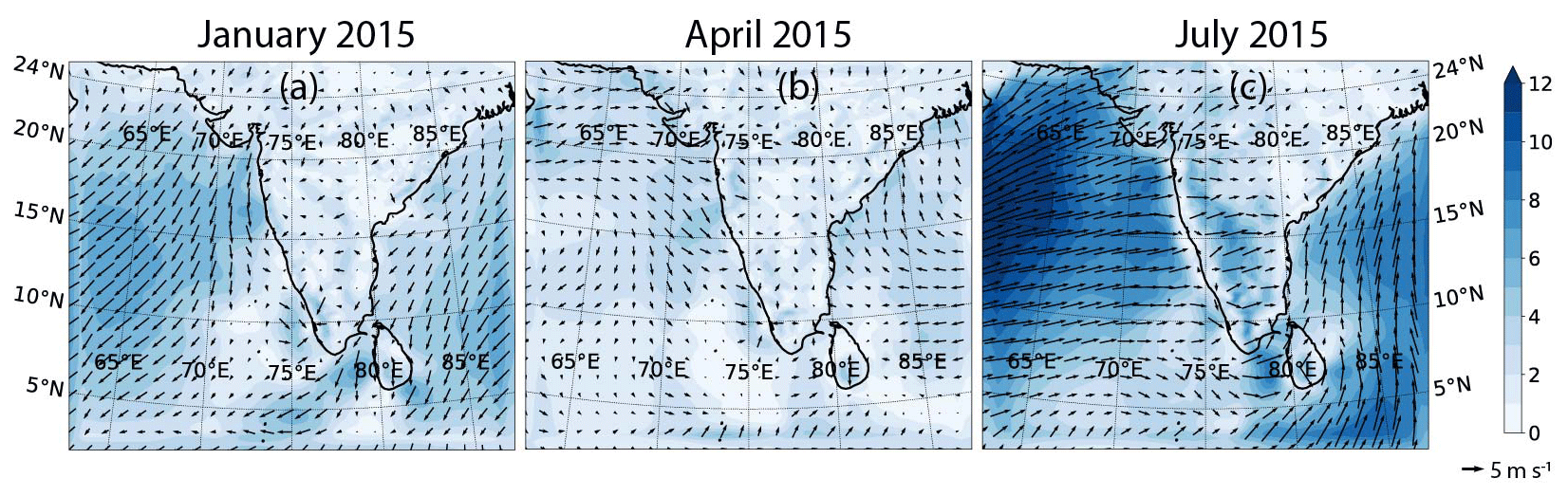
Figure 1The wind direction and speed over the model domain during the 3 months used to study the impact of iodine chemistry on the marine boundary layer. The 3 months represent different seasons: the winter monsoon period in January, pre-monsoon in April, and the summer monsoon in July. The direction of the arrows shows the wind direction, and the size of the arrows and the contour colours show the magnitude of the wind.
The WRF-Chem model (version 3.7.1), which included a full halogen scheme (Cl, Br, and I), was used in the present study. The halogen chemistry scheme used in WRF-Chem and a detailed description of the model set-up are given in past studies (Badia et al., 2019; Li et al., 2020). The bromine and chlorine chemistry schemes were kept the same through all the simulations. Sources of reactive iodine species considered in this study are an oceanic source of organic iodine compounds (CH2ICl, CH2IBr, CH2I2, and CH3I) and inorganic compounds from the ocean surface (HOI and I2). The sea-to-air fluxes of organic compounds were calculated online (Liss and Slater, 1974). The oceanic emission of inorganic iodine (HOI and I2), which is dependent on the deposition of O3 to the surface ocean and reaction with iodide (I−), was calculated online using a parameterization based on Badia et al. (2019), which was computed using the empirical laboratory-measured parameterizations by Carpenter et al. (2013) and MacDonald et al. (2014). These emissions produced much-higher-than-observed levels of IO in the northern Indian Ocean MBL. The reasons for the overestimation are discussed further in Sect. 3.2. Hence for the rest of the analysis, the emissions of I2 and HOI were reduced by 40 % (i.e. 60 % of the standard emission parameterization). Iodine species, including INO3, HOI, HI, IBr, ICl, INO2, I2, I2O2, I2O3, and I2O4, undergo a washout process as described in Badia et al. (2019) and the reference therein. The simulated washout of atmospheric compositions (here taking O3 as an example) in these 3 months (Jan, Apr, and Jul) are shown in Fig. S1 in the Supplement. The washout intensity is lower in the pre-monsoon season (Apr) and higher in the monsoon seasons (Jan and Jul). Potential uncertainty in other model configurations, e.g. washout process, could also lead to uncertainties in the simulated abundance of iodine species.
The domain for the simulations was selected to cover the Indian subcontinent and the northern Indian Ocean (as shown in Fig. 1). We used a spatial resolution of 27 km and 30 vertical layers (sigma levels of 1.00, 0.99, 0.98, 0.97, 0.96, 0.95, 0.94, 0.93, 0.92, 0.91, 0.89, 0.85, 0.78, 0.70, 0.60, 0.51, 0.43, 0.36, 0.31, 0.27, 0.23, 0.20, 0.17, 0.14, 0.11, 0.08, 0.05, 0.03, 0.02, 0.01, 0.00) with the surface layer ∼ 20 and 10 layers within the boundary layer. The simulation period included three seasons in the year of 2015 (pre-monsoon in April, summer monsoon in July, and the winter monsoon period in January). We ran the WRF-Chem model for the months of January, April, and July with an extra spin-up period of 15 d. The reason for choosing these 3 months is the different chemical regimes that result over the Indian Ocean due to changing meteorological conditions. Figure 1 shows the monthly averaged wind direction and speed over the northern Indian Ocean, which shows large differences in the transport of air masses over the three seasons. Using these considerations, three sets of simulations were conducted. The BASE scenario considered no iodine emissions from the ocean surface, the orgI scenario considered only emissions of organoiodides as mentioned above, and the HAL scenario considered emissions of both inorganic iodine and the organoiodides. Changes in atmospheric compositions between BASE and HAL represent the impact of the overall iodine sources and chemistry, while those between the BASE and orgI scenarios represent the impact of organic iodine emissions, and the difference between orgI and HAL shows the impact of inorganic emissions of iodine from the ocean surface (HOI and I2).
The model results were validated using daily averaged observations from cruise-based campaigns in the Indian Ocean, i.e. during the 2nd International Indian Ocean Expedition (December 2015) and the 8th Indian Southern Ocean Expedition (ISOE-8) (January 2015) (Mahajan et al., 2019b, a). Unfortunately, observations were available only during the winter monsoon period, and hence no direct validation was possible during the other seasons. Observations of IO in the MBL, along with surface ozone concentrations, were used for the validation of the model simulations. The MBL in the model results was defined as the lowest 10 layers (1.0 ). The domain chosen for the model simulations, along with the tracks of the cruises from which data were used for validation, is shown in Fig. 2.
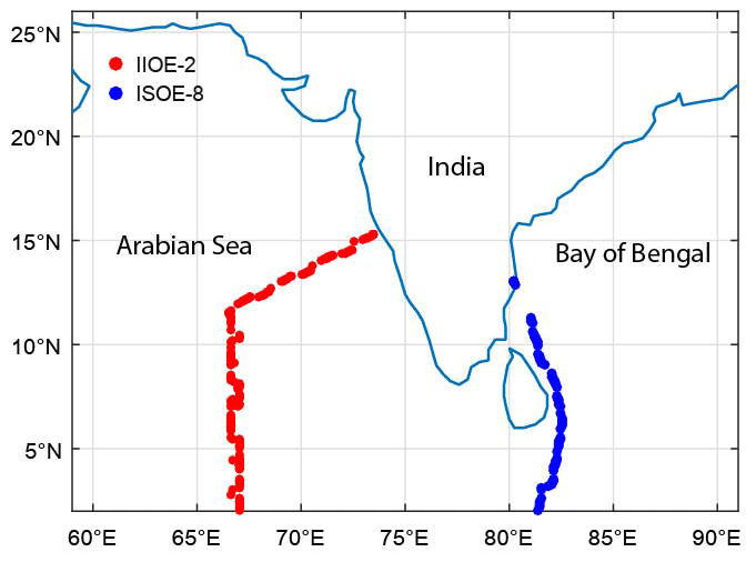
Figure 2The domain chosen for the model runs, along with the tracks of the cruises from which data were used for validation, is shown. The two cruises were the 2nd International Indian Ocean Expedition (IIOE-2; December 2015) and the 8th Indian Southern Ocean Expedition (ISOE-8; January 2015) and started from the western and eastern coast of India, respectively.
3.1 Model validation
A comparison between the model-simulated IO and O3 from the HAL scenario and observations made during the IIOE-2 and ISOE-8 expeditions is shown in Fig. 3. Figure 3a shows a comparison between the modelled and observed IO mixing ratios, with both the model and observations showing IO values below 1 pptv for all the locations. For most of the data points, the model-simulated IO is slightly higher than the observations, although within the uncertainty. It should be remembered that this close match is after reducing the emissions of inorganic iodine species from the ocean surface by 40 % (discussed further in Sect. 3.2). The largest mismatch is observed close to 5∘ N, where the model predicts approximately 0.9 pptv, while the observations show a low of 0.23 ± 0.16 pptv. A point to note is that the IIOE-2 observations were from December 2015, and hence an exact match is not expected. Nonetheless, the comparison shows that the model does a good job at reproducing the levels of IO observed in the northern Indian Ocean. The levels of observed and simulated IO are similar to the eastern Pacific (Badia et al., 2019) and in the South China Sea (Li et al., 2020) but lower than the modelled and observed values of ∼ 1.5 pptv in the tropical Atlantic MBL (Mahajan et al., 2010b).
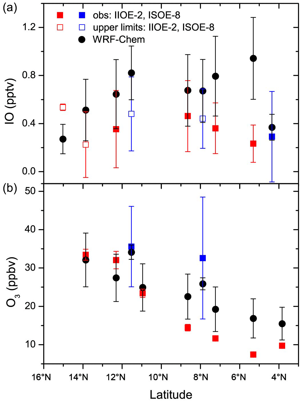
Figure 3A comparison between the model-simulated and observed daily averaged IO (a) and O3 (b) as per the cruise locations is shown. In cases where IO was not detected, an upper limit (empty squares; the errors in the empty squares show the range of upper limits for that day) was estimated. The model validation was performed only for the winter period, when the cruise-based data were available.
Figure 3b shows a comparison between the model-simulated O3 with the observations. Although the match between the model and observations is good in the northern Indian Ocean, there is a mismatch in the open ocean closer to the Equator, with the model predicting higher values than the observations. The decreasing trend towards the open ocean is well captured by the model, with higher values observed close to the Indian coast, where larger anthropogenic emissions are present. The average overestimation of ozone across all the locations where observations were available was ∼ 25 %. The model captures well the difference between the IIOE-2 and the ISOE-8 cruises, which started from the western and eastern coasts of India, respectively. Larger values of O3 were observed during the ISOE-8, which were seen in the model simulations too and show that the O3 concentrations during the winter months are higher to the east of India as compared to the west.
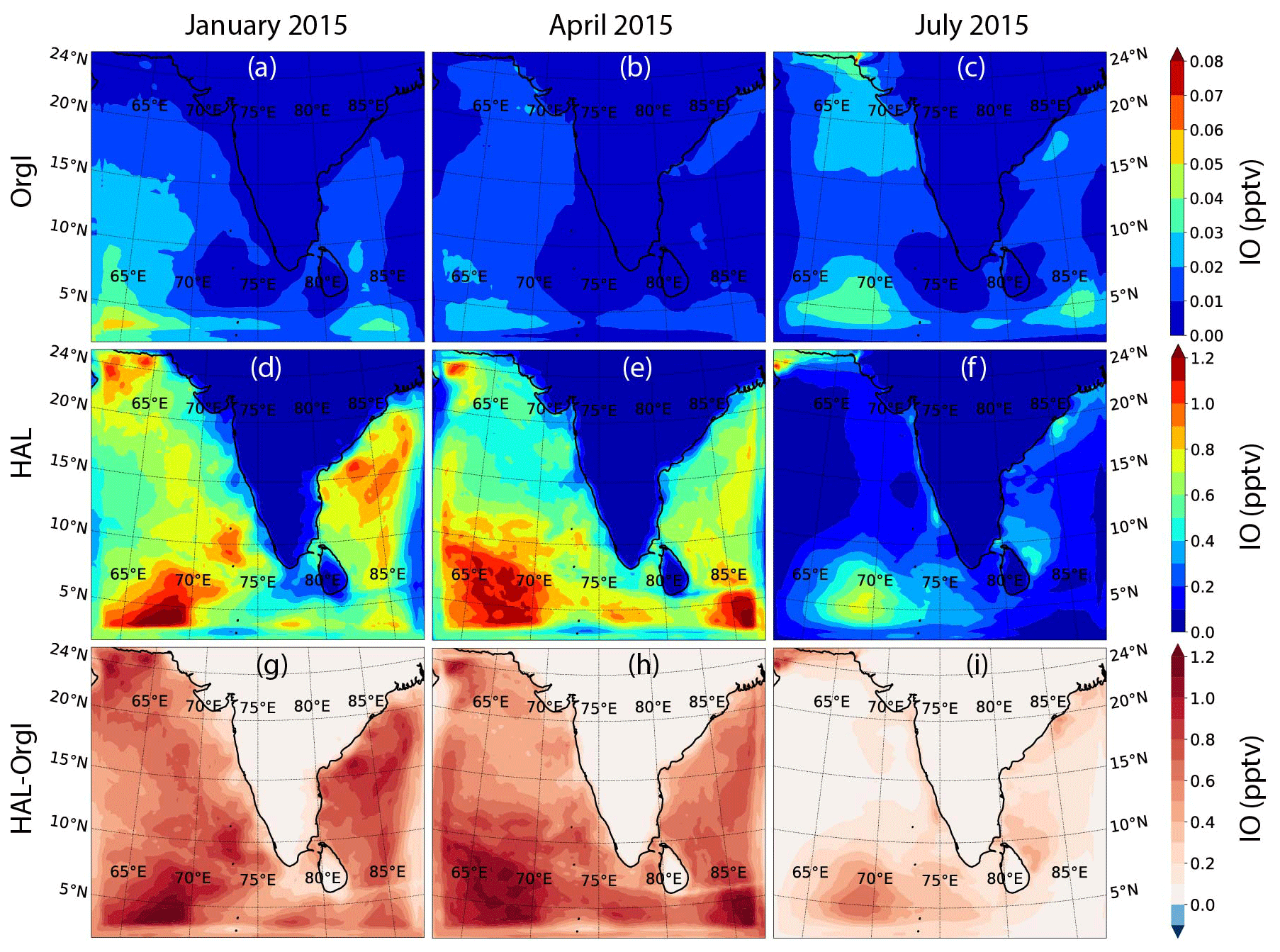
Figure 4Model simulation showing the boundary-layer-averaged IO mixing ratios across the domain during the three seasons, along with a difference between the HAL and orgI scenarios for each season.
3.2 Geographical distribution of IO
Figure 4 shows the geographical distribution of daytime-averaged IO across the selected domain during the three seasons for the orgI and HAL cases, along with the difference between the two. The orgI scenario shows significantly low values across the domain, with a peak of only 0.06 pptv (in January) in the western Indian Ocean close to the Equator (Fig. 4a–c). When averaged across the whole domain for the boundary layer, the mean IO mixing ratio is a negligible 0.011 ± 0.009 pptv in January, 0.008 ± 0.006 pptv in April, and 0.012 ± 0.009 pptv in July (Table 1). Even if only the MBL is considered after applying a land mask, the mean IO mixing ratio is only 0.015 ± 0.009 pptv in January, 0.011 ± 0.006 pptv in April, and 0.015 ± 0.008 pptv in July (Table 1). At such low concentrations, iodine chemistry does not have any measurable impact on atmospheric chemistry. The values closer to the Indian subcontinent are negligible, although a high of ∼ 0.04 pptv is seen close to the western Indian and Pakistani coasts during the summer monsoon period (July). It is well known that this region experiences strong mixing in the northern Arabian sea during the summer monsoon period, which triggers plankton blooms, resulting in high productivity (Qasim, 1982). For the current model runs, emissions of organic iodine are based on a climatology concentration of organic halogens in the seawater (Ziska et al., 2013), which show high organoiodide emissions in this region. However, despite being an area of high productivity, the values of IO predicted in the orgI scenarios are significantly lower than the observations by a factor of 10–20 (Fig. 4) and show the need for an inorganic iodine flux. Such a flux has been suggested to be ubiquitous and dependent on the ozone deposition and seawater iodide concentrations (Carpenter et al., 2013; MacDonald et al., 2014).
Table 1Monthly mean of IO concentration in parts per trillion by volume (pptv) over the domain region for model simulations in January, April, and July 2015 and simulation scenarios orgI and HAL as well as the difference between HAL and orgI before and after applying a land mask over the model domain.

Figure 4d–f show the distribution of IO for the HAL scenario, which includes an inorganic iodine flux of I2 and HOI as mentioned earlier. The flux strength has been reduced by 40 % (i.e. 60 % of the standard emission parameterization) compared to the past studies to get a closer match between the observations and the model. Without such a reduction, the model predicts a peak of ∼ 1.7 pptv in the domain, which is almost double the peak value observed during the IIOE-2 or ISOE-8, even when the uncertainty in the observations is considered (Fig. 3). The main drivers for a sea-to-air flux of HOI and I2 are the concentration of iodide in the seawater and the atmospheric ozone concentrations. The seawater iodide concentration in the model was estimated using the MacDonald et al. (2014) parameterization, which is based on the sea surface temperature. This is also the largest uncertainty in the inorganic iodine emissions parameterization. Recent studies have shown that the MacDonald et al. parameterization underestimates the seawater iodide in the Indian Ocean (Inamdar et al., 2020), with the model-predicted mean iodide in the domain being 117.4 ± 1.4 nM (range: 113 to 119 nM). Ship-based observations in the same region show a mean iodide value of 185.8 ± 66.0 nM (range of 100 to 320 nM) (Chance et al., 2019, 2020). Iodide observations were unfortunately not made during the same time as the model runs, but it is unlikely that the model overestimates the iodide considering the range of reported observations. Indeed, if we use the mean observed values for the seawater iodide concentrations, the I2 flux would increase by ∼ 58 %, and HOI flux would increase by 44 % rather than both decrease by 40 % as necessary. The second potential reason for overestimating the sea-to-air iodine flux could be the overestimation of ozone in the model. The model overestimates the ozone by ∼ 25 % across all the locations where ozone observations were available (Fig. 3). This would cause a ∼ 20 % larger flux of HOI and I2 as compared to the observed O3 values. However, reducing the flux by 20 % is still not enough for the model to match the observations. Other uncertainties in the calculation of the inorganic iodine flux calculation are in Henry's law of HOI, which has not been measured but is estimated. Past reports in the Indian Ocean have also questioned the accuracy of the parameterization-based sea-to-air flux of iodine species in the Indian Ocean (Inamdar et al., 2020; Mahajan et al., 2019a). The current model results also suggest that the accuracy of the flux needs to be revisited, and direct flux observations, which have not been made to date, would be helpful in quantification of the inorganic iodine emissions.
Additionally, there are other sources of uncertainties which could contribute to the mismatch. For example, the treatment of the heterogeneous chemistry has large uncertainties in their uptake coefficients associated with the ability of the model to simulate the aerosol size distribution (and aerosol surface area) and the mixing state and surface composition of the atmospheric aerosols. The photochemistry of I2Ox species also represents an important source of uncertainty in the iodine chemical mechanism incorporated into chemistry transport models (Lewis et al., 2020; Saiz-Lopez and von Glasow, 2012; Sommariva et al., 2012). However, a new set of IxOy photodepletion experiments have recently been reported but have not been incorporated in the available model mechanisms (Lewis et al., 2020). A further uncertainty in the IO concentration calculation is that most chemical transport models tend to underestimate the sources of nitrogen in the open ocean, resulting in lower levels of NOx in the MBL (e.g. Travis et al., 2020), which could lead to higher mixing ratios of IO. Observations of NOx in the MBL are rare given the low concentrations, and no observations have been made in the Indian Ocean MBL. However, an increase in NOx would lead to an increase in the ozone, which is already slightly overestimated in the model.

Figure 5The boundary-layer-averaged O3 mixing ratios across the domain during the three seasons for the HAL scenario (a–c), along with the differences (d–f) and the percentage differences (g–i) between the HAL and BASE scenarios for each season.
Using a reduced flux, seasonally, the highest levels of IO across the domain are observed during the winter monsoon period in January, and the lowest levels are observed during the summer monsoon period in July (Fig. 4). While higher values (between 0.7–0.9 pptv) are observed in the Bay of Bengal compared to the Arabian Sea, a clear peak in IO is seen close to 3∘ N in the western Indian Ocean, between 65∘ E and 70∘ E. This high is even more prominent during the pre-monsoon season in April, with the peak monthly averaged values reaching as high as 1.3 pptv. A similar high is also observed during April in the eastern part of the domain close to the Equator. A strong seasonal variation is seen, with IO values significantly lower in July as compared to January and April. July is the summer monsoon period and is characterized by cleaner air over the domain, with clean oceanic air coming from the south-west (Fig. 1). This leads to a reduction in the concentrations of pollutants in the MBL. Considering that the emission of inorganic iodine is driven by the deposition of O3 at the surface, the reduction in IO can be attributed to a lower concentration of O3 in the MBL in July (Fig. 5). When averaged over the entire domain, the mean IO mixing ratios are 0.47 ± 0.32 pptv in January, 0.48 ± 0.33 pptv in April, and 0.15 ± 0.15 pptv in July, showing the strong seasonality driven by the emission of inorganic iodine compounds from the ocean surface. The main reason for this season change is the emissions of HOI and I2 rather than due to deposition effects as we can see significant changes in the HOI and I2 emissions also during July (Fig. S2 in the Supplement). When a land mask is applied, and a mean only over the MBL is computed, the values increased to 0.63 ± 0.20 pptv in January, 0.64 ± 0.22 pptv in April, and 0.19 ± 0.14 pptv in July. These values are higher than the means across the entire domain, showing that most of the IO is restricted to the MBL, close to the oceanic sources. The concentrations of IO in the current domain are lower than levels predicted by past studies in other environments. Using a similar set-up to the current study in WRF-Chem, Badia et al. (2019) estimated IO levels of 0.5 pptv in the subtropics as compared to about 0.8 pptv in the tropics in the MBL. Li et al. (2020) predicted higher levels in the south China Sea, with IO values ranging between 1–3 pptv. By comparison, results from the Community Multiscale Air Quality Modelling System (CMAQ) predicted peaks of 4–7 pptv in the coastal regions around Europe, while the open-ocean concentrations were below 1 pptv (Li et al., 2019). Thus, in comparison, the values in the Indian Ocean are lower, especially in July, than other regions studied hitherto using regional models, implying a reduced impact of iodine chemistry on the atmosphere in the northern Indian Ocean environment.
Figure 4g–i show the difference in IO between the HAL and orgI scenarios. During January and April, the differences are large, with most of the IO being contributed by the inorganic emissions. The largest differences (∼ 1.2 pptv) are observed in locations where a peak is seen in the HAL scenario, closer to the Equator. During July, the differences are smaller, with most of the open-ocean MBL showing a smaller increase compared to the other seasons when the inorganic flux is included. It should however be remembered that even though the differences in July are only as high as 0.5 pptv, the orgI scenario predicts only up to 0.04 pptv during this season, which is lower by an order of magnitude. Seasonally also, the difference between the two scenarios is large, with the domain-averaged IO mixing ratios showing values of 0.46 ± 0.31 pptv in January, 0.47 ± 0.32 pptv in April, and 0.14 ± 0.14 pptv in July for the HAL − orgI contribution. When a land mask is applied, and a mean only over the MBL is computed, the values are 0.62 ± 0.20 pptv in January, 0.63 ± 0.21 pptv in April, and 0.18 ± 0.14 pptv in July. This suggests that most of the IO in the Indian Ocean MBL is due to emissions of inorganic iodine compounds rather than the photolysis of organoiodides, which are longer-lived than the inorganic species and hence do not contribute heavily to the MBL. A similar result has been observed in other oceanic MBLs, where observations show that a small fraction of the total IO in the MBL is due to organic compounds (Mahajan et al., 2010b).
Figure S3 in the Supplement shows the vertical distribution of IO as simulated in the HAL scenario for the January month in the region between 2–10∘ N and 65–73∘ E close to the Equator, where the higher values are observed. Most of the IO is restricted to the boundary layer, with the IO mixing ratio reducing to less than a 10th of the value of the surface above the boundary layer. This indicates that most of the iodine in the model is indeed from short-lived gases, HOI and I2 being the primary source.
For the rest of the analysis, we use the difference between the HAL and BASE scenarios to quantify the impact of iodine chemistry considering that the orgI greatly underestimates the iodine concentrations in the model domain. The differences and percentage differences in oxidizing species such as ozone (O3), nitrogen oxides (NO2 and NO), hydrogen oxides (OH and HO2), and the nitrate radical (NO3) are studied to quantify the impact of iodine on the MBL atmosphere.
Table 2Monthly means and standard deviations of O3, NO2, NO, NO3, OH, and HO2 mixing ratios (unit in parentheses) over the domain region for the model simulations in January, April, and July for the HAL scenario along with the difference and percentage differences between HAL and BASE. The table also includes monthly mean values only over the MBL.

3.3 Impact on ozone
Figure 5 shows the geographical distribution of O3 across the selected domain during the three seasons for the HAL scenario, along with the absolute and percentage difference between the HAL and BASE scenarios. A steady decrease is observed from the coast to the open-ocean environment, which is expected considering that the main sources of O3 are emitted on the subcontinent. Seasonal changes are observed, with higher concentrations observed during January and April as compared to the summer monsoon period. During January and April, the winds flow from the subcontinent towards the open ocean, while during July the winds flow from the open ocean towards the subcontinent, which results in cleaner air masses during July (Fig. 1). Additionally, during the summer monsoon, wet deposition also plays a role in the removal of O3 and its precursors from the atmosphere. During January, higher values are observed in the MBL, which is due to stronger winds advecting the polluted air masses from the continent (Fig. 1). The model also predicts higher values of O3 over the Bay of Bengal as compared to the Arabian Sea, which was also seen in the observations (Fig. 3). The lowest values are seen during the monsoon period, when cleaner oceanic air is seen over the whole domain and only the MBL (Table 2). This shows that the advection of anthropogenic sources from the continent affects the ozone in the remote MBL too (Table 2).
Figure 5d–f show the absolute difference in O3 (HAL − BASE) over the model domain. During January and April significant ozone destruction is observed in the MBL, with as much as 3.5 ppbv less O3 in the HAL scenario as compared to the BASE scenario. During January relatively larger destruction is observed in the Bay of Bengal as compared to the Arabian Sea. Significant losses in O3 are also observed in the western Indian Ocean closer to the Equator. Interestingly, O3 destruction is also visible over the Indian subcontinent, showing that the effects of iodine chemistry are not just limited to the MBL. In January, an increase of 1 ppbv is seen over the south of India. During April, the destruction of O3 is more restricted to the MBL, with larger destruction observed in the Arabian Sea as compared to the Bay of Bengal. The main difference in the O3 during these 2 months is driven by the dynamics, which dictates where the oceanic emissions of iodine are advected. During July, a negligible difference is observed between the HAL and BASE case, with the depletion within ± 0.3 ppbv, which reflects the lower concentrations of iodine during the summer monsoon period. When averaged over the entire domain, the mean change in O3 mixing ratios shows a reduction in January and April, but in July there is a statistically non-significant increase when the IO concentrations are very low. This change in ozone is mainly driven by changes in the MBL, where the differences are the largest between the HAL and BASE scenarios. If we consider the absolute changes (|HAL − BASE|), defined as the mean of the absolute difference rather than the mean change, the differences are significantly larger (Table S1 in the Supplement). The reason for larger absolute differences as compared to mean differences is that there are both increases and decreases seen in different parts of the domain, and hence the absolute differences gives us an idea of the total impact of iodine chemistry.
Figure 5g–i show the percentage change in O3 between the BASE and HAL scenarios. A reduction in the O3 concentrations of as much as 20 % is observed in the MBL when iodine chemistry is included, with the largest differences observed in the western part of the domain, closer to the Equator. For most of the domain, the change in O3 is < 15 %. Over the Indian subcontinent and close to the coastal areas, the relative change in O3 is small, which is due to larger absolute concentrations in these locations. In January and July, a small increase (< 5 %) in the O3 concentrations is predicted over large parts of the domain. This shows the non-linear effect of iodine chemistry on the atmosphere, which can lead to an increase in O3 in certain parts of the domain due to changes in other oxidants. When averaged over the entire domain, the largest relative change is seen during the winter period in January followed by the pre-monsoon season in April, while the smallest change is in July during the monsoon, when the IO values are low (Table 2). Over the MBL, the mean percentage changes in O3 mixing show larger differences, confirming that most of the impacts of iodine chemistry on ozone destruction are seen in the MBL (Table 2). The fact that the absolute change values are close to the mean change values shows that most of the domain sees a destruction in ozone due to the presence of iodine compounds (Table S1).
This relative change is lower than in the Pacific, where the WRF-Chem-simulated O3 destruction because of all halogens peaked at −16 ppbv, which was approximately 70 % of the total ozone loss, of which 18 %–23 % was because of iodine chemistry (Badia et al., 2019). The loss of O3 due to iodine was similar to the current domain in China, where the change in ozone because of all halogens was −10 % to +5 % (Li et al., 2020). Over Europe, combined halogen chemistry, which includes I, Br, and Cl, significantly reduces the concentrations of O3 by as much as 10 ppbv. The contribution because of only iodine is also larger than in the current domain, which is expected because of the higher IO concentrations simulated in Europe (Li et al., 2019) and the iodine source parameterization being reduced in this study.
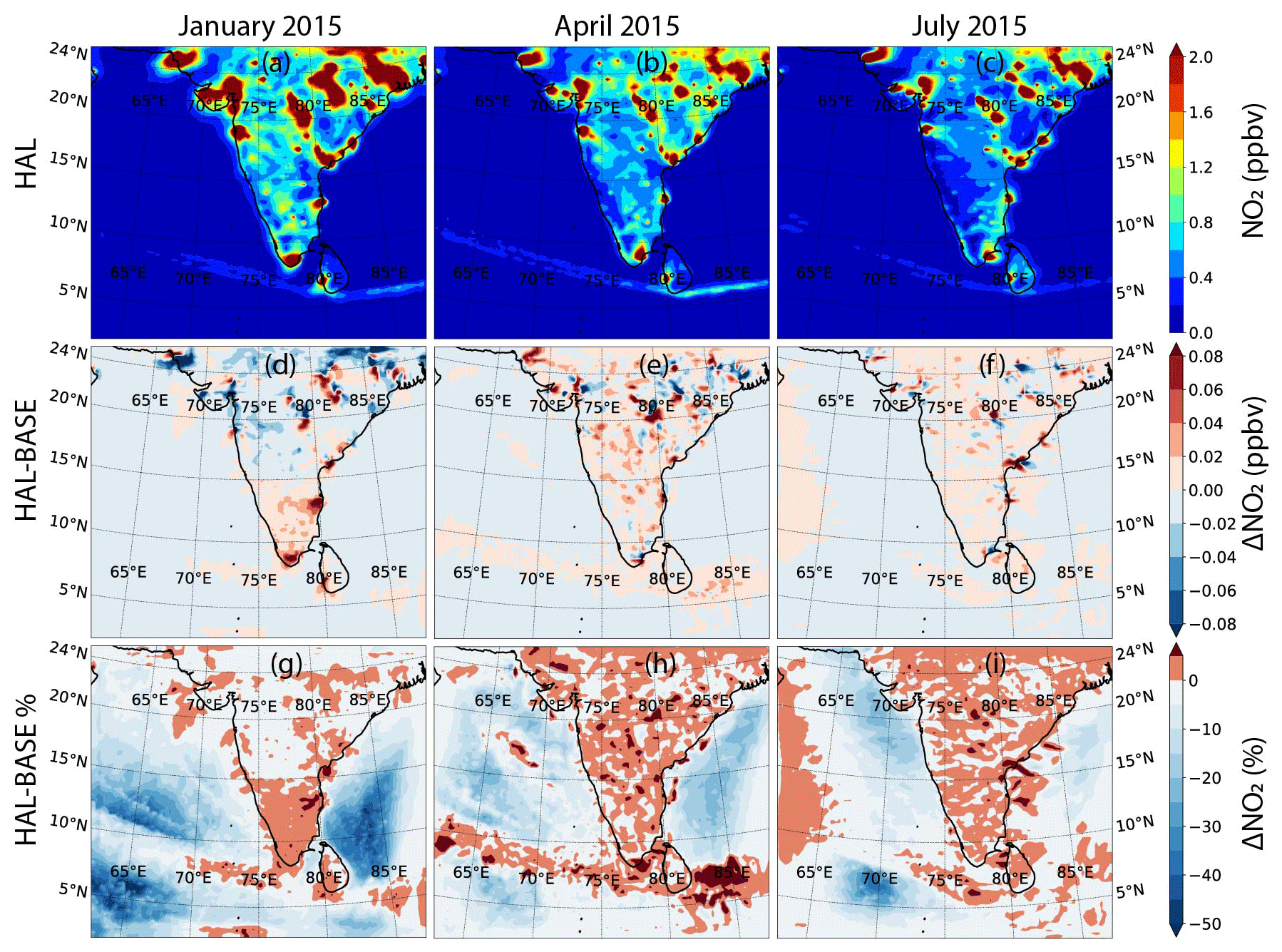
Figure 6NO2 mixing ratios averaged in the boundary layer across the domain during the three seasons for the HAL scenario (a–c), along with the differences (d–f) and the percentage differences (g–i) between the HAL and BASE scenarios for each season.
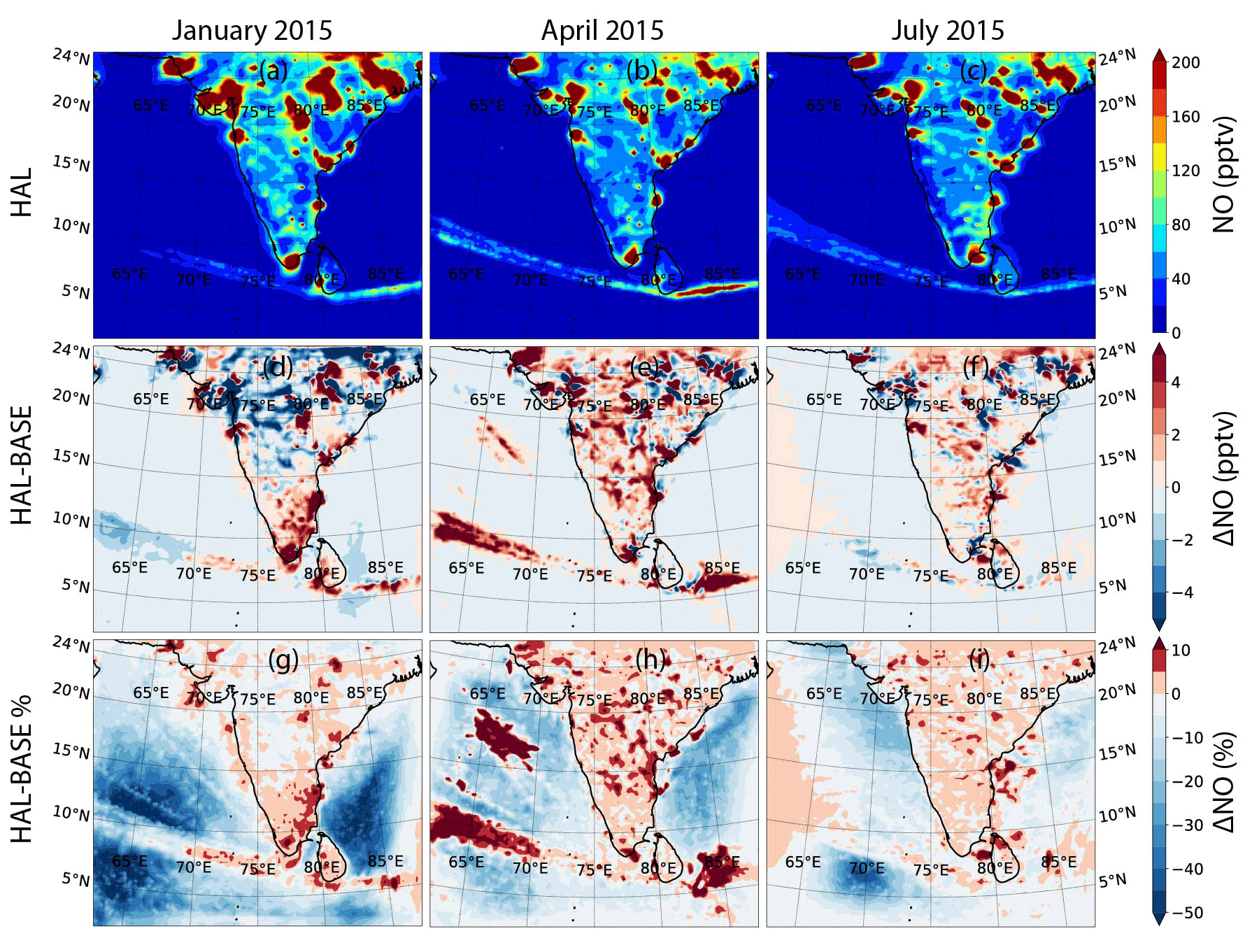
Figure 7Mean boundary layer NO mixing ratios across the domain during the three seasons for the HAL scenario (a–c), along with the differences (d–f) and the percentage differences (g–i) between the HAL and BASE scenarios for each season.
3.4 Impact on nitrogen oxides (NOx)
Halogen oxides interact with nitrogen oxides to change the ratio by reacting with NO to form NO2. Additionally, iodine oxides can also react with NOx to form iodine nitrate (IONO2), which can be taken up on aerosol surfaces to act as a sink or recycle both nitrogen compounds and iodine compounds (Atkinson et al., 2007). Thus, the resultant change in nitrogen oxides depends on the concentrations of iodine compounds, concentrations of nitrogen compounds, and the aerosol surface available for heterogenous recycling. Figures 6 and 7 show the geographical distribution of NO2 and NO across the selected domain during the three seasons for the HAL scenario, along with the absolute and percentage difference between the HAL and BASE scenarios. A sharp decrease is observed from the coast to the open-ocean environment. The shipping lanes in the Indian Ocean also show higher concentrations of NO2 and are clearly visible, especially south of the Indian subcontinent, where NO2 mixing ratios of up to 1 ppbv can be seen. A seasonal variation is also observed, with higher concentrations observed during winter in January, followed by the pre-monsoon period in April, with the summer monsoon period in July showing the lowest concentrations, even at the hotspots. When averaged over the entire domain, the lowest values are observed during the monsoon period, when cleaner oceanic air is seen over the domain (Table 2).
NO mixing ratios peak over 400 pptv in the subcontinent as compared to mixing ratios less than 20 pptv in large parts of the MBL (Fig. 7). The hotspots for NO, which coincide with the hotspots for NO2, are also clearly visible. A sharp decrease is observed from the coast to the open-ocean environment like NO2, indicating that fossil fuel combustion over land is the main source. The shipping lanes in the Indian Ocean are noticeable, with NO mixing ratios of up to 200 pptv observed in some regions. The seasonal variation for NO follows the same trend as NO2, with higher concentrations observed during January, followed by April, with the summer monsoon period in July showing the lowest concentrations. However, January shows the lowest concentrations in the shipping lanes. Large standard deviations show that the high concentrations of NO are mainly restricted to hotspots, which leads to a large variation across the domain. Over only the MBL, the mean mixing ratios are lower and have smaller standard deviations, which shows that the MBL is much cleaner than the air above the Indian subcontinent and does not contain large hotspots, although it is affected by the coastal regions (Table 2).
Figures 6d–f and 7d–f show the absolute difference in NO2 and NO for the HAL and BASE scenarios. For NO2, a small reduction is observed in most of the MBL during all the months, with changes of about −0.04 ppbv observed at most locations. Over the subcontinent, there is variation observed at some locations, with decreases and increases showing a maximum of ± 0.08 ppbv. Over the shipping lanes, where high NO2 is observed, an increase of about 0.04 ppbv is observed after the inclusion of iodine chemistry. In the case of NO, the variation observed is similar to NO2, with a small reduction observed in most of the MBL during all the months, with changes of about −2 pptv observed at most locations. Over the subcontinent, significant variation is also observed for NO, with decreases and increases showing a maximum of ± 8 pptv. In most of the shipping lanes, where high NO is observed, the inclusion of iodine chemistry leads to an increase in the NOx concentrations, especially in April, where the increase in NO2 can be as high as ∼ 10 %, and the increase in NO can be as high as 15 %. Similarly to NO2, the change due to IO can be ascertained to be larger when the mean absolute differences instead of just the mean differences are considered.
Significant differences are observed over the MBL, with decreases in NOx as high as 50 % over large areas when iodine chemistry is included (Figs. 6 and 7). The largest differences are observed in the western Arabian Sea and in the southern Bay of Bengal. Over the Indian subcontinent and close to the coastal areas, the relative change in both NO2 and NO is small due to larger absolute concentrations in these locations, although a small increase is observed over most of the land area. In the shipping lanes, NOx mostly shows an increase, which is due to the recycling of halogen nitrates on the aerosol surfaces. The large standard deviations in the mean changes highlight the huge variability in the average values. The inclusion of iodine chemistry leads to the reduction in NO2 in the domain, albeit with a large variation, which would contribute to the reduction in O3 as mentioned above since NO2 is the main source of ozone in the MBL. When we consider the mean absolute change to see the actual impact of iodine chemistry, the values of the means are much higher, with as much as ∼ 3.5 % change in NO2 and 7 % change in NO observed over the MBL (Table S1). This change in NOx is smaller than simulated in Europe, with NO2 predicted to increase across most of Europe and most regions showing an increase between 50–200 pptv. However, this was the increase reported due to the inclusion of all the halogens, and the impact of only iodine would be lower, even though higher levels were simulated across Europe (Li et al., 2019).
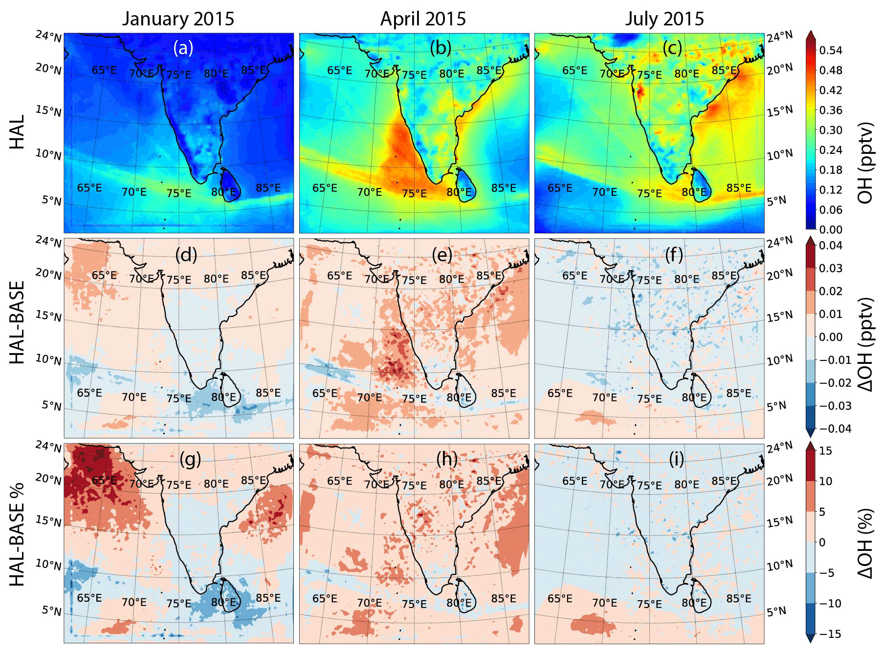
Figure 8OH mixing ratios across the domain during the three seasons for the HAL scenario (a–c), along with the differences (d–f) and the percentage differences (g–i) between the HAL and BASE scenarios for each season.
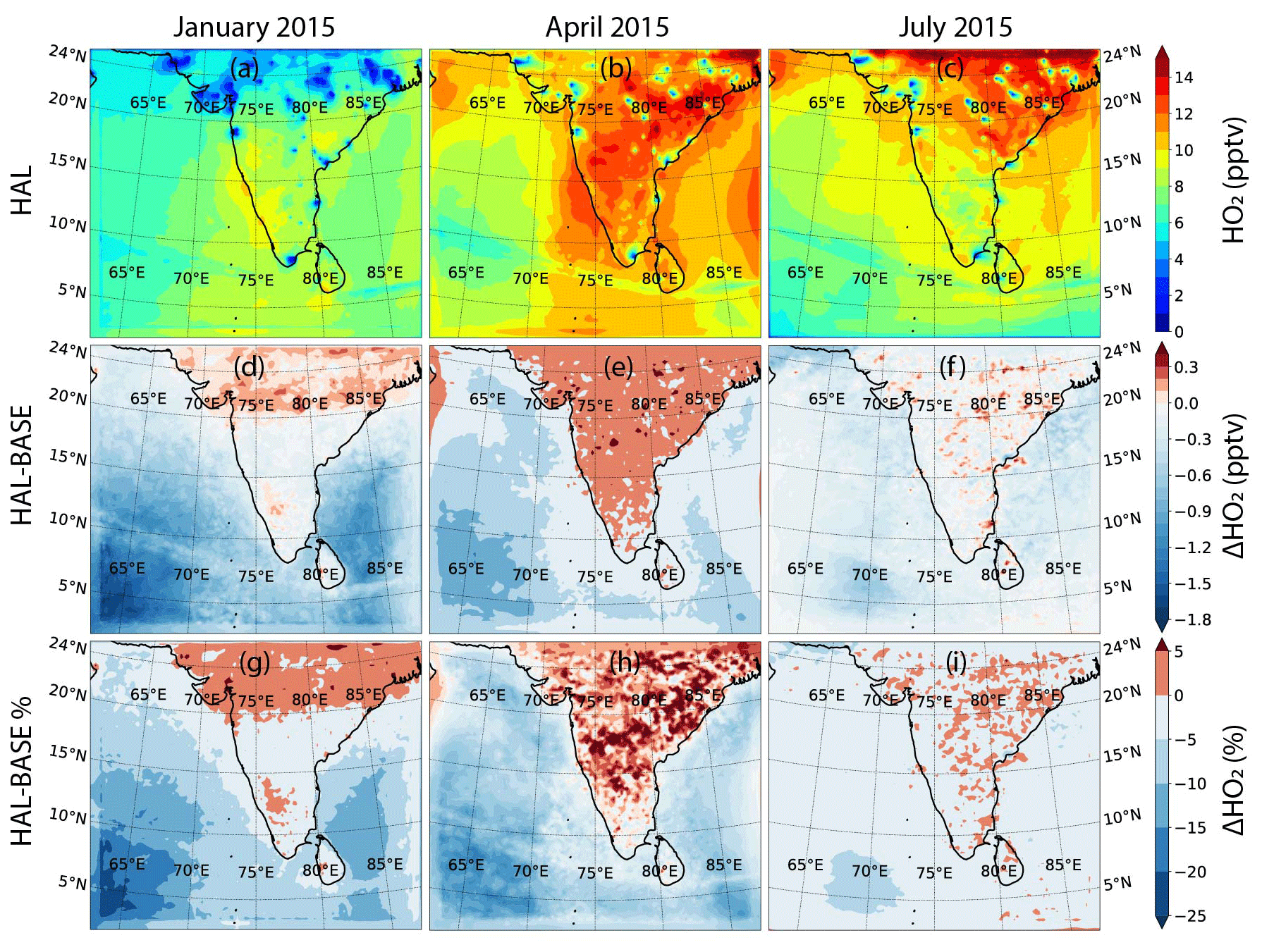
Figure 9Model simulations showing the boundary-layer-averaged HO2 mixing ratios across the domain during the three seasons for the HAL scenario (a–c), along with the differences (d–f) and the percentage differences (g–i) between the HAL and BASE scenarios for each season.
3.5 Impact on hydrogen oxides (HOx)
Hydrogen oxides are impacted by iodine chemistry through the catalytic reaction involving IO changing HO2 into OH. This leads to an increase in the oxidizing capacity of the atmosphere due to an increase in the OH concentrations. Figures 8 and 9 show the geographical distribution of OH and HO2 across the selected domain during the three seasons for the HAL scenario, along with the absolute and percentage differences between the HAL and BASE scenarios. The daily averaged OH mixing ratios peak at about 0.5 pptv in the MBL close to the Indian subcontinent, as compared to mixing ratios less than 0.3 pptv over most of the subcontinent (Fig. 8). The shipping lanes in the Indian Ocean show higher concentrations of OH and are clearly visible, especially south of the Indian subcontinent and in the Arabian Sea, where OH mixing ratios of up to 0.45 pptv can be seen. A strong seasonal variation is observed as expected, with higher concentrations observed during the months of April and July and the winter period in January showing the lowest concentrations. This annual variation is driven by the availability of solar radiation, which is a critical component in OH production.
HO2 shows much higher concentrations over the Indian subcontinent as compared to the surrounding ocean MBL, with HO2 mixing ratios peaking over 15 pptv in the subcontinent as compared to mixing ratios less than 10 pptv over most of the MBL (Fig. 9). A gradual decrease in the HO2 mixing ratios is observed from the subcontinent to the open-ocean environment during the months of April and July, although the HO2 concentrations in the MBL are larger during January. Relatively, the winter month of January shows the lowest HO2 mixing ratios of the 3 months. The shipping lanes in the Indian Ocean are clearly visible like for OH, although the HO2 concentrations in the shipping lanes are lower than the surrounding areas. This is due to the titration of HO2 by ship-emitted NO mentioned earlier, which leads to an increase in OH but a decrease in HO2.
Figures 8d–f and 9d–f show the absolute difference in OH and HO2. For OH, a small increase in the OH concentration is observed in most of the MBL during the months of January and April, with the largest increase of about 0.03 pptv observed in the Arabian Sea. However, for most of the domain, the increase in OH is small, with differences of 0.01 pptv compared to the BASE scenario. During the monsoon month of July, a small decrease is observed over most of the domain, with an increase observed further south, close to the Equator. Over the shipping lanes, a small reduction is observed during all the months, with changes of about −0.02 pptv along the ship tracks. In the case of HO2, a clear land–ocean contrast is observed in the differences, with the HO2 values reducing over the entire MBL but showing a small increase over the subcontinent. The largest reduction is observed in the south-western Arabian Sea, with changes of about −1.8 pptv in the HAL scenario as compared to the BASE case. Seasonally, the largest changes in HO2 are observed in January, with the least changes observed in the monsoon month of July. IO concentrations are the lowest during monsoon due to clean air-masses reducing the ozone-deposition-driven emissions, and hence the difference between the HAL and BASE scenarios is also the lowest during July. When averaged over the whole domain, the mean change in OH mixing ratios is negligible. In the case of HO2, the average difference over the whole domain is also small, but over the MBL too the differences are larger, with the largest difference being −0.67 ± 0.36 pptv in January (Table 2).
Figures 8g–i and 9g–i show the percentage changes in OH and HO2 between the HAL and BASE scenarios. Significant differences are observed, with an increase in OH and a decrease in the HO2 over most of the MBL. The largest change in OH is observed in the northern Arabian Sea MBL, with a difference of more than 15 % between the HAL and BASE cases when iodine chemistry is included. Large parts of the Arabian Sea and the Bay of Bengal show an increase in OH of up to 10 % for January and April, with a smaller difference observed in July due to lower concentrations of iodine compounds in the atmosphere. In January and April, when the concentrations of IO are higher, a negative change in the OH concentrations is observed over the shipping lanes. In the case of HO2, a large change of up to −25 % is observed in the MBL, with the largest differences observed in the south-western Arabian Sea, close to the Equator. During the months of January and April, most of the MBL shows a change of −10 % to −20 %, while a positive change of 0 %–5 % is observed over the Indian subcontinent. The mean percentage change in the OH and HO2 mixing ratios peaks at 2.6 % and 8.4 % for the months of April and January, respectively (Table 2). For example, the 3.29 % increase in the OH concentrations observed across the domain in January (Table S1) would result in the lowering of the methane lifetime by 3.19 % in the MBL (assuming = 1.85 × 10⁻¹² ; Atkinson et al., 2006). A similar change in the oxidizing capacity has been simulated in other parts of the world, with halogen chemistry inducing complex effects on OH (ranging from −0.023 to 0.030 pptv) and HO2 (in the range of −3.7 to 0.73 pptv) in Europe (Li et al., 2019) and enhancing the total atmospheric oxidation capacity in polluted areas of China, typically 10 % to 20 % (up to 87 % in winter) and mainly by significantly increasing OH levels (Li et al., 2020). The moderate increase in the oxidation capacity over the northern Indian Ocean and the Indian subcontinent is due to the lower concentrations of IO in the domain, along with the fact that this number is calculated only for the impact of iodine chemistry, while the past studies have reported the impact of all halogens. Globally the average increase in OH because of the inclusion of iodine chemistry has been estimated to be 1.8 %, which is comparable to the current domain (Sherwen et al., 2016).
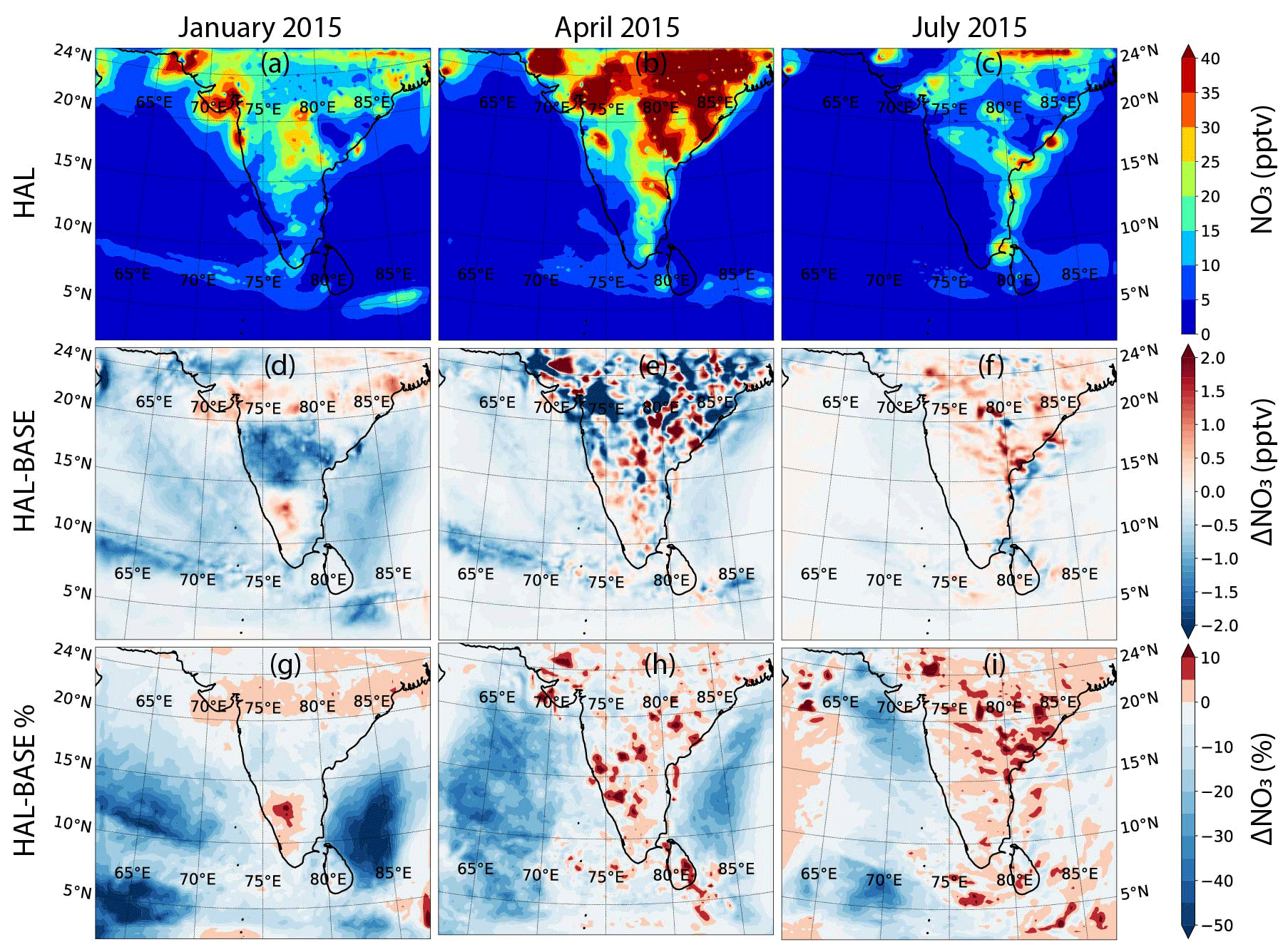
Figure 10NO3 mixing ratios across the domain during the three seasons for the HAL scenario (a–c), along with the differences (d–f) and the percentage differences (g–i) between the HAL and BASE scenarios for each season.
3.6 Impact on the nitrate radical (NO3)
NO3 radicals are the predominant night-time oxidant and play a similar role to OH during the daytime in the degradation of atmospheric constituents (Wayne et al., 1991). Iodine compounds interact with NO3, mainly through the primary emissions of inorganic iodine compounds by the oxidation of chemicals such as I2 and HOI (Saiz-Lopez et al., 2016). Figure 10 shows the geographical distribution of NO3 across the selected domain during the three seasons, for the HAL scenario, along with the absolute and percentage difference between the HAL and BASE scenarios. As expected, much higher concentrations of NO3 are observed over the Indian subcontinent as compared to the surrounding ocean MBL, with NO3 mixing ratios peaking over 40 pptv in the subcontinent as compared to mixing ratios less than 5 pptv in the MBL surrounding the Indian subcontinent. A sharp decrease is observed from the coast to the open-ocean environment, which is expected considering that the main sources of NO3 are on the subcontinent and NO3 has a short lifetime due to its high reactivity. The seasonal variation is the same as O3, with peak values observed over the Indian subcontinent over the month of April, followed by January. The monsoon month of July displays the lowest concentrations due to efficient removal of NOx and O3 due to wet deposition. Elevated values up to 15 pptv are also observed along the shipping lanes due to the conversion of ship-emitted NOx into NO3 during the night-time. The lowest values are observed during the monsoon period, similarly to O3, when cleaner oceanic air is observed over the domain (Table 2). If only the MBL, where lower concentrations of NOx are observed, is considered, the mean NO3 mixing ratios are much lower (Table 2).
Figure 10d–f show the absolute difference in NO3 over the model domain. During the months of January and April, a significant reduction of up to −1.5 pptv is observed in the MBL. During January, a reduction is observed in the Bay of Bengal as well as the Arabian Sea, but in April the reduction in NO3 is largely observed in the Arabian Sea. This correlates well with the IO distribution, which also shows more iodine activity in the Arabian Sea during April. A reduction in NO3 is also visible over the Indian subcontinent and like O3 shows that the effects of iodine chemistry are not just limited to the MBL. Indeed, there are pockets of an increase in NO3 observed over the subcontinent. During July, negligible difference is observed between the HAL and BASE case, with a decrease of less than 0.5 pptv seen across the MBL. However, during the same period, an increase of up to 1.5 pptv can be seen over the NOx hotspots over the Indian subcontinent. Decreases of up to −1.5 pptv are also observed along the shipping lanes, showing the strong interaction between iodine and NOx chemistry. Over the whole domain, the inclusion of iodine chemistry results in a mean decrease of about ∼ −0.4 pptv, which is slightly higher when a mean is taken only for the MBL (Table 2). The absolute change in NO3 is even higher, with NO3 values changing by an average of 0.5 pptv across the whole domain in July (Table S1). This value is however lower than the effect of all the halogens, as shown by Li et al. (2019) in Europe, where halogens significantly reduced the concentrations of NO3 by as much as 20 pptv.
Figure 10g–i show the percentage change in NO3 between the BASE and HAL scenarios. As much as a 50 % reduction in the NO3 concentrations is observed in the MBL when iodine chemistry is included, with the largest differences observed in the Arabian Sea, close to the Indian subcontinent, further west closer to the Equator, and in the Bay of Bengal. For most of the other domain, the change in NO3 is < 20 %. Over the Indian subcontinent, the relative change in NO3 is small due to larger absolute concentrations, and in some places a small increase (< 5 %) is predicted, especially in July, when iodine chemistry is not highly active. The relative change in the shipping lanes is smaller than the surrounding areas due to the higher relative concentrations of NO3 along the tracks (< 20 %). On average, the inclusion of iodine chemistry can cause an almost 10 % change in the NO3 concentrations across the MBL in January, with smaller changes of ∼ 4.5 % observed during July, when the IO concentrations are lower (Table S1).
In this study, we used the WRF-Chem regional model to quantify the impacts of the observed levels of iodine on the chemical composition of the MBL over the northern Indian Ocean. The model was validated with observations from two cruises during the winter season. The model results show that the IO concentrations are greatly underestimated if only organic iodine compound emissions are considered in the model. This reaffirms that emissions of inorganic species resulting from the deposition of ozone on the sea surface are needed to reproduce the observed levels of IO. However, the current parameterizations overestimate the concentrations, which could be because of a combination of modelling uncertainties and the HOI and I2 flux parameterization not being directly applicable to this region. This agrees with previous reports in the Indian Ocean questioning the current parameterizations and highlights the need for direct HOI and I2 flux observations. For a reasonable match with cruise-based observations, the inorganic emissions had to be reduced by 40 %. The simulations after this reduction in flux show a strong seasonal variation, with lower iodine concentrations predicted when cleaner air is found over the Indian subcontinent due to flushing by remote oceanic air masses during the monsoon season, but higher iodine concentrations are predicted during the winter period, when polluted air from the Indian subcontinent increases the ozone concentrations in the MBL. A large regional variation is observed in the IO distribution and also in the impacts of iodine chemistry. Iodine-catalysed reactions can lead to significant regional changes, with peaks of 25 % destruction in O3, altering the NOx concentrations by up to 50 %, increasing the OH concentration by as much as 15 %, reducing the HO2 concentration by as much as 25 %, and causing a change of up to 50 % in the nitrate radical (NO3). When averaged across the whole domain, the differences are smaller, although still significant. For example, the average change in OH across the whole domain reduces the methane lifetime by ∼ 3 % in the MBL, showing the impact of iodine on the oxidation capacity. Most of the large relative changes are observed in the open-ocean MBL, but iodine chemistry also affects the chemical composition in the coastal environment and over the Indian subcontinent. Indeed, in some instances an increase in O3 concentrations is predicted over the subcontinent, showing the non-linear effects. These model results highlight the importance of iodine chemistry in the northern Indian Ocean and suggest that it needs to be included in future studies for improved accuracy in modelling the chemical composition in this region.
The analysis codes for extracting data from the WRF-Chem outputs are available at https://doi.org/10.17632/jc8wtyx5sg.1 (Mahajan, 2021). WRF-Chem is a community model available from NCAR (https://www2.acom.ucar.edu/wrf-chem, last access: June 2021) (NCAR, 2021).
The data used in this publication are available at https://doi.org/10.17632/jc8wtyx5sg.1 (Mahajan, 2021).
The supplement related to this article is available online at: https://doi.org/10.5194/acp-21-8437-2021-supplement.
ASM conceptualized the research plan and methodology, analysed the data, and wrote the paper. QL did the model runs for the study and contributed towards the interpretation of the results and writing. SI helped with the analysis, interpretation, and writing. KR, AB, and ASL contributed towards the interpretation and writing.
The authors declare that they have no conflict of interest.
The IITM is funded by the Ministry of Earth Sciences (MOES), government of India. This study has been funded by the European Research Council Executive Agency under the European Union's Horizon 2020 research and innovation programme (project “ERC-2016-COG 726349 CLIMAHAL”).
This paper was edited by Jens-Uwe Grooß and reviewed by Rolf Sander and one anonymous referee.
Alicke, B., Hebestreit, K., Stutz, J., and Platt, U.: Iodine oxide in the marine boundary layer, Nature, 397, 572–573, https://doi.org/10.1038/17508, 1999.
Allan, B. J., McFiggans, G., Plane, J. M. C., and Coe, H.: Observations of iodine monoxide in the remote marine boundary layer, J. Geophys. Res.-Atmos., 105, 14363–14369, https://doi.org/10.1029/1999JD901188, 2000.
Allan, J. D., Williams, P. I., Najera, J., Whitehead, J. D., Flynn, M. J., Taylor, J. W., Liu, D., Darbyshire, E., Carpenter, L. J., Chance, R., Andrews, S. J., Hackenberg, S. C., and McFiggans, G.: Iodine observed in new particle formation events in the Arctic atmosphere during ACCACIA, Atmos. Chem. Phys., 15, 5599–5609, https://doi.org/10.5194/acp-15-5599-2015, 2015.
Atkinson, R., Baulch, D. L., Cox, R. A., Crowley, J. N., Hampson, R. F., Hynes, R. G., Jenkin, M. E., Rossi, M. J., and Troe, J.: Evaluated kinetic and photochemical data for atmospheric chemistry: Volume III – gas phase reactions of inorganic halogens, Atmos. Chem. Phys., 7, 981–1191, https://doi.org/10.5194/acp-7-981-2007, 2007.
Atkinson, R., Baulch, D. L., Cox, R. A., Crowley, J. N., Hampson, R. F., Hynes, R. G., Jenkin, M. E., Rossi, M. J., Troe, J., and Wallington, T. J.: Evaluated kinetic and photochemical data for atmospheric chemistry: Volume IV – gas phase reactions of organic halogen species, Atmos. Chem. Phys., 8, 4141–4496, https://doi.org/10.5194/acp-8-4141-2008, 2008.
Baccarini, A., Karlsson, L., Dommen, J., Duplessis, P., Vüllers, J., Brooks, I. M., Saiz-Lopez, A., Salter, M., Tjernström, M., Baltensperger, U., Zieger, P., and Schmale, J.: Frequent new particle formation over the high Arctic pack ice by enhanced iodine emissions, Nat. Commun., 11, 1–11, https://doi.org/10.1038/s41467-020-18551-0, 2020.
Badia, A., Reeves, C. E., Baker, A. R., Saiz-Lopez, A., Volkamer, R., Koenig, T. K., Apel, E. C., Hornbrook, R. S., Carpenter, L. J., Andrews, S. J., Sherwen, T., and von Glasow, R.: Importance of reactive halogens in the tropical marine atmosphere: a regional modelling study using WRF-Chem, Atmos. Chem. Phys., 19, 3161–3189, https://doi.org/10.5194/acp-19-3161-2019, 2019.
Bloss, W. J., Lee, J. D., Johnson, G. P., Sommariva, R., Heard, D. E., Saiz-Lopez, A., Plane, J. M. C., McFiggans, G., Coe, H., Flynn, M., Williams, P., Rickard, A. R., and Fleming, Z. L.: Impact of halogen monoxide chemistry upon boundary layer OH and HO2 concentrations at a coastal site, Geophys. Res. Lett., 32, 1–4, https://doi.org/10.1029/2004GL022084, 2005.
Carpenter, L. J.: Iodine in the marine boundary layer, Chem. Rev., 103, 4953–4962, https://doi.org/10.1021/Cr0206465, 2003.
Carpenter, L. J., MacDonald, S. M., Shaw, M. D., Kumar, R., Saunders, R. W., Parthipan, R., Wilson, J., and Plane, J. M. C.: Atmospheric iodine levels influenced by sea surface emissions of inorganic iodine, Nat. Geosci., 6, 108–111, https://doi.org/10.1038/ngeo1687, 2013.
Chameides, W. L. and Davis, D. D.: Iodine: Its possible role in tropospheric photochemistry, J. Geophys. Res., 85, 7383–7398, https://doi.org/10.1029/JC085iC12p07383, 1980.
Chance, R., Tinel, L., Sherwen, T., Baker, A., Bell, T., Brindle, J., Campos, M. L. A. M., Croot, P., Ducklow, H., He, P., Hoogakker, B., Hopkins, F. E., Hughes, C., Jickells, T., Loades, D., Macaya, D. A., Mahajan, A. S., Malin, G., Phillips, D. P., Sinha, A. K., Sarkar, A., Roberts, I. J., Roy, R., Song, X., Winklebauer, H. A., Wuttig, K., Yang, M., Zhou, P., and Carpenter, L. J.: Global sea-surface iodide observations, 1967–2018, Nat. Sci. Data, 6, https://doi.org/10.1038/s41597-019-0288-y, 2019.
Chance, R., Tinel, L., Sarkar, A., Sinha, A. K., Mahajan, A. S., Chacko, R., Sabu, P., Roy, R., Jickells, T. D., Stevens, D. P., Wadley, M., and Carpenter, L. J.: Surface Inorganic Iodine Speciation in the Indian and Southern Oceans From 12∘ N to 70∘ S, Front. Mar. Sci., 7, 1–16, https://doi.org/10.3389/fmars.2020.00621, 2020.
Commane, R., Seitz, K., Bale, C. S. E., Bloss, W. J., Buxmann, J., Ingham, T., Platt, U., Pöhler, D., and Heard, D. E.: Iodine monoxide at a clean marine coastal site: observations of high frequency variations and inhomogeneous distributions, Atmos. Chem. Phys., 11, 6721–6733, https://doi.org/10.5194/acp-11-6721-2011, 2011.
Cuevas, C. A., Maffezzoli, N., Corella, J. P., Spolaor, A., Vallelonga, P., Kjær, H. A., Simonsen, M., Winstrup, M., Vinther, B., Horvat, C., Fernandez, R. P., Kinnison, D., Lamarque, J.-F., Barbante, C., and Saiz-Lopez, A.: Rapid increase in atmospheric iodine levels in the North Atlantic since the mid-20th century, Nat. Commun., 9, 1452, https://doi.org/10.1038/s41467-018-03756-1, 2018.
Furneaux, K. L., Whalley, L. K., Heard, D. E., Atkinson, H. M., Bloss, W. J., Flynn, M. J., Gallagher, M. W., Ingham, T., Kramer, L., Lee, J. D., Leigh, R., McFiggans, G. B., Mahajan, A. S., Monks, P. S., Oetjen, H., Plane, J. M. C., and Whitehead, J. D.: Measurements of iodine monoxide at a semi polluted coastal location, Atmos. Chem. Phys., 10, 3645–3663, https://doi.org/10.5194/acp-10-3645-2010, 2010.
Gómez Martín, J. C., Mahajan, A. S., Hay, T. D., Prados-Román, C., Ordóñez, C., MacDonald, S. M., Plane, J. M. C., Sorribas, M., Gil, M., Paredes Mora, J. F., Agama Reyes, M. V., Oram, D. E., Leedham, E., and Saiz-Lopez, A.: Iodine chemistry in the eastern Pacific marine boundary layer, J. Geophys. Res.-Atmos., 118, 887–904, https://doi.org/10.1002/jgrd.50132, 2013.
Großmann, K., Frieß, U., Peters, E., Wittrock, F., Lampel, J., Yilmaz, S., Tschritter, J., Sommariva, R., von Glasow, R., Quack, B., Krüger, K., Pfeilsticker, K., and Platt, U.: Iodine monoxide in the Western Pacific marine boundary layer, Atmos. Chem. Phys., 13, 3363–3378, https://doi.org/10.5194/acp-13-3363-2013, 2013.
Iglesias-Suarez, F., Kinnison, D. E., Rap, A., Maycock, A. C., Wild, O., and Young, P. J.: Key drivers of ozone change and its radiative forcing over the 21st century, Atmos. Chem. Phys., 18, 6121–6139, https://doi.org/10.5194/acp-18-6121-2018, 2018.
Inamdar, S., Tinel, L., Chance, R., Carpenter, L. J., Sabu, P., Chacko, R., Tripathy, S. C., Kerkar, A. U., Sinha, A. K., Bhaskar, P. V., Sarkar, A., Roy, R., Sherwen, T., Cuevas, C., Saiz-Lopez, A., Ram, K., and Mahajan, A. S.: Estimation of reactive inorganic iodine fluxes in the Indian and Southern Ocean marine boundary layer, Atmos. Chem. Phys., 20, 12093–12114, https://doi.org/10.5194/acp-20-12093-2020, 2020.
Lawrence, M. G. and Lelieveld, J.: Atmospheric pollutant outflow from southern Asia: a review, Atmos. Chem. Phys., 10, 11017–11096, https://doi.org/10.5194/acp-10-11017-2010, 2010.
Legrand, M., McConnell, J. R., Preunkert, S., Arienzo, M., Chellman, N., Gleason, K., Sherwen, T., Evans, M. J., and Carpenter, L. J.: Alpine ice evidence of a three-fold increase in atmospheric iodine deposition since 1950 in Europe due to increasing oceanic emissions, P. Natl. Acad. Sci. USA, 115, 12136–12141, https://doi.org/10.1073/pnas.1809867115, 2018.
Lelieveld, J., Crutzen, P. J., Ramanathan, V., Andreae, M. O., Brenninkmeijer, C. A. M., Campos, T., Cass, G. R., Dickerson, R. R., Fischer, H., De Gouw, J. A., Hansel, A., Jefferson, A., Kley, D., De Laat, A. T. J., Lal, S., Lawrence, M. G., Lobert, J. M., Mayol-Bracero, O. L., Mitra, A. P., Novakov, T., Oltmans, S. J., Prather, K. A., Reiner, T., Rodhe, H., Scheeren, H. A., Sikka, D., and Williams, J.: The Indian Ocean Experiment: Widespread air pollution from South and Southeast Asia, Science, 291, 1031–1036, https://doi.org/10.1126/science.1057103, 2001.
Lewis, T. R., Gómez Martín, J. C., Blitz, M. A., Cuevas, C. A., Plane, J. M. C., and Saiz-Lopez, A.: Determination of the absorption cross sections of higher-order iodine oxides at 355 and 532 nm, Atmos. Chem. Phys., 20, 10865–10887, https://doi.org/10.5194/acp-20-10865-2020, 2020.
Li, Q., Borge, R., Sarwar, G., de la Paz, D., Gantt, B., Domingo, J., Cuevas, C. A., and Saiz-Lopez, A.: Impact of halogen chemistry on summertime air quality in coastal and continental Europe: application of the CMAQ model and implications for regulation, Atmos. Chem. Phys., 19, 15321–15337, https://doi.org/10.5194/acp-19-15321-2019, 2019.
Li, Q., Badia, A., Wang, T., Sarwar, G., Fu, X., Zhang, L., Zhang, Q., Fung, J., Cuevas, C. A., Wang, S., Zhou, B., and Saiz-Lopez, A.: Potential Effect of Halogens on Atmospheric Oxidation and Air Quality in China, J. Geophys. Res.-Atmos., 125, e2019JD032058, https://doi.org/10.1029/2019jd032058, 2020.
Liss, P. S. and Slater, P. G.: Flux of gases across air-sea interface, Nature, 247, 181–184, 1974.
MacDonald, S. M., Gómez Martín, J. C., Chance, R., Warriner, S., Saiz-Lopez, A., Carpenter, L. J., and Plane, J. M. C.: A laboratory characterisation of inorganic iodine emissions from the sea surface: dependence on oceanic variables and parameterisation for global modelling, Atmos. Chem. Phys., 14, 5841–5852, https://doi.org/10.5194/acp-14-5841-2014, 2014.
Mahajan, A.: Modelling the impacts of iodine chemistry on the northern Indian Ocean marine boundary layer, Mendeley Data, V1, https://doi.org/10.17632/jc8wtyx5sg.1, 2021.
Mahajan, A. S., Oetjen, H., Saiz-Lopez, A., Lee, J. D., McFiggans, G. B., and Plane, J. M. C.: Reactive iodine species in a semi-polluted environment, Geophys. Res. Lett., 36, L16803, https://doi.org/10.1029/2009GL038018, 2009.
Mahajan, A. S., Shaw, M., Oetjen, H., Hornsby, K. E., Carpenter, L. J., Kaleschke, L., Tian-Kunze, X., Lee, J. D., Moller, S. J., Edwards, P. M., Commane, R., Ingham, T., Heard, D. E., and Plane, J. M. C.: Evidence of reactive iodine chemistry in the Arctic boundary layer, J. Geophys. Res., 115, D20303, https://doi.org/10.1029/2009JD013665, 2010a.
Mahajan, A. S., Plane, J. M. C., Oetjen, H., Mendes, L., Saunders, R. W., Saiz-Lopez, A., Jones, C. E., Carpenter, L. J., and McFiggans, G. B.: Measurement and modelling of tropospheric reactive halogen species over the tropical Atlantic Ocean, Atmos. Chem. Phys., 10, 4611–4624, https://doi.org/10.5194/acp-10-4611-2010, 2010b.
Mahajan, A. S., Sorribas, M., Gómez Martín, J. C., MacDonald, S. M., Gil, M., Plane, J. M. C., and Saiz-Lopez, A.: Concurrent observations of atomic iodine, molecular iodine and ultrafine particles in a coastal environment, Atmos. Chem. Phys., 11, 2545–2555, https://doi.org/10.5194/acp-11-2545-2011, 2011.
Mahajan, A. S., Gómez Martín, J. C., Hay, T. D., Royer, S.-J., Yvon-Lewis, S., Liu, Y., Hu, L., Prados-Roman, C., Ordóñez, C., Plane, J. M. C., and Saiz-Lopez, A.: Latitudinal distribution of reactive iodine in the Eastern Pacific and its link to open ocean sources, Atmos. Chem. Phys., 12, 11609–11617, https://doi.org/10.5194/acp-12-11609-2012, 2012.
Mahajan, A. S., Tinel, L., Hulswar, S., Cuevas, C. A., Wang, S., Ghude, S., Naik, R. K., Mishra, R. K., Sabu, P., Sarkar, A., Anilkumar, N., and Saiz Lopez, A.: Observations of iodine oxide in the Indian Ocean marine boundary layer: A transect from the tropics to the high latitudes, Atmos. Environ., 1, 100016, https://doi.org/10.1016/j.aeaoa.2019.100016, 2019a.
Mahajan, A. S., Tinel, L., Sarkar, A., Chance, R., Carpenter, L. J., Hulswar, S., Mali, P., Prakash, S., and Vinayachandran, P. N.: Understanding Iodine Chemistry over the Northern and Equatorial Indian Ocean, J. Geophys. Res.-Atmos., 124, 8104–8118, https://doi.org/10.1029/2018JD029063, 2019b.
McFiggans, G. B.: Marine aerosols and iodine emissions, Nature, 433, E13–E13, 2005.
Muñiz-Unamunzaga, M., Borge, R., Sarwar, G., Gantt, B., de la Paz, D., Cuevas, C. A., and Saiz-Lopez, A.: The influence of ocean halogen and sulfur emissions in the air quality of a coastal megacity: The case of Los Angeles, Sci. Total Environ., 610–611, 1536–1545, https://doi.org/10.1016/j.scitotenv.2017.06.098, 2018.
NCAR: WRF-Chem, available at: https://www2.acom.ucar.edu/wrf-chem, last access: June 2021.
O'Dowd, C. D., Jimenez, J. L., Bahreini, R., Flagan, R. C., Seinfeld, J. H., Hämeri, K., Pirjola, L., Kulmala, M., Gerard Jennings, S., Hoffmann, T., Hameri, K., and Jennings, S. G.: Marine aerosol formation from biogenic iodine emissions, Nature, 417, 632–636, https://doi.org/10.1038/nature00775, 2002.
O'Dowd, C. D., Facchini, M. C., Cavalli, F., Ceburnis, D., Mircea, M., Decesari, S., Fuzzi, S., Yoon, Y. J., Putaud, J. P., and Dowd, C. D. O.: Biogenically driven organic contribution to marine aerosol, Nature, 431, 676–680, https://doi.org/10.1038/nature02970.1., 2004.
Platt, U. and Honninger, G.: The role of halogen species in the troposphere, Chemosphere, 52, 325–338, 2003.
Platt, U. and Janssen, C.: Observation and Role of the Free Radicals NO3 CI0, BrO and I0 in the Troposphere, Faraday Discuss., 100, 175–198, 1995.
Prados-Roman, C., Cuevas, C. A., Hay, T., Fernandez, R. P., Mahajan, A. S., Royer, S.-J., Galí, M., Simó, R., Dachs, J., Großmann, K., Kinnison, D. E., Lamarque, J.-F., and Saiz-Lopez, A.: Iodine oxide in the global marine boundary layer, Atmos. Chem. Phys., 15, 583–593, https://doi.org/10.5194/acp-15-583-2015, 2015.
Qasim, S. Z.: Oceanography of the northern Arabian Sea, Deep-Sea Res., 29, 1041–1068, https://doi.org/10.1016/0198-0149(82)90027-9, 1982.
Read, K. A., Mahajan, A. S., Carpenter, L. J., Evans, M. J., Faria, B. V. E., Heard, D. E., Hopkins, J. R., Lee, J. D., Moller, S. J., Lewis, A. C., Mendes, L. M., McQuaid, J. B., Oetjen, H., Saiz-Lopez, A., Pilling, M. J., and Plane, J. M. C.: Extensive halogen-mediated ozone destruction over the tropical Atlantic Ocean, Nature, 453, 1232–1235, https://doi.org/10.1038/nature07035, 2008.
Sahu, L. K., Lal, S., and Venkataramani, S.: Distributions of O3, CO and hydrocarbons over the Bay of Bengal: A study to assess the role of transport from southern India and marine regions during September–October 2002, Atmos. Environ., 40, 4633–4645, https://doi.org/10.1016/j.atmosenv.2006.02.037, 2006.
Saiz-Lopez, A. and Plane, J. M. C.: Novel iodine chemistry in the marine boundary layer, Geophys. Res. Lett., 31, L04112, https://doi.org/10.1029/2003GL019215, 2004.
Saiz-Lopez, A. and von Glasow, R.: Reactive halogen chemistry in the troposphere, Chem. Soc. Rev., 41, 6448–6472, https://doi.org/10.1039/c2cs35208g, 2012.
Saiz-Lopez, A., Mahajan, A. S., Salmon, R. A., Bauguitte, S. J.-B., Jones, A. E., Roscoe, H. K., and Plane, J. M. C.: Boundary Layer Halogens in Coastal Antarctica, Science, 317, 348–351, https://doi.org/10.1126/science.1141408, 2007.
Saiz-Lopez, A., Plane, J. M. C., Baker, A. R., Carpenter, L. J., von Glasow, R., Martín, J. C. G., McFiggans, G. B., Saunders, R. W., and Gómez Martín, J. C.: Atmospheric Chemistry of Iodine, Chem. Rev., 112, 1773–1804, https://doi.org/10.1021/cr200029u, 2012a.
Saiz-Lopez, A., Lamarque, J.-F., Kinnison, D. E., Tilmes, S., Ordóñez, C., Orlando, J. J., Conley, A. J., Plane, J. M. C., Mahajan, A. S., Sousa Santos, G., Atlas, E. L., Blake, D. R., Sander, S. P., Schauffler, S., Thompson, A. M., and Brasseur, G.: Estimating the climate significance of halogen-driven ozone loss in the tropical marine troposphere, Atmos. Chem. Phys., 12, 3939–3949, https://doi.org/10.5194/acp-12-3939-2012, 2012b.
Saiz-Lopez, A., Fernandez, R. P., Ordóñez, C., Kinnison, D. E., Gómez Martín, J. C., Lamarque, J.-F., and Tilmes, S.: Iodine chemistry in the troposphere and its effect on ozone, Atmos. Chem. Phys., 14, 13119–13143, https://doi.org/10.5194/acp-14-13119-2014, 2014.
Saiz-Lopez, A., Plane, J. M. C., Cuevas, C. A., Mahajan, A. S., Lamarque, J.-F., and Kinnison, D. E.: Nighttime atmospheric chemistry of iodine, Atmos. Chem. Phys., 16, 15593–15604, https://doi.org/10.5194/acp-16-15593-2016, 2016.
Sarwar, G., Gantt, B., Schwede, D., Foley, K., Mathur, R., and Saiz-Lopez, A.: Impact of Enhanced Ozone Deposition and Halogen Chemistry on Tropospheric Ozone over the Northern Hemisphere, Environ. Sci. Technol., 49, 9203–9211, https://doi.org/10.1021/acs.est.5b01657, 2015.
Seitz, K., Buxmann, J., Pöhler, D., Sommer, T., Tschritter, J., Neary, T., O'Dowd, C., and Platt, U.: The spatial distribution of the reactive iodine species IO from simultaneous active and passive DOAS observations, Atmos. Chem. Phys., 10, 2117–2128, https://doi.org/10.5194/acp-10-2117-2010, 2010.
Sellegri, K., Pey, J., Rose, C., Culot, A., DeWitt, H. L., Mas, S., Schwier, A. N., Temime-Roussel, B., Charriere, B., Saiz-Lopez, A., Mahajan, A. S., Parin, D., Kukui, A., Sempere, R., D'Anna, B., and Marchand, N.: Evidence of atmospheric nanoparticle formation from emissions of marine microorganisms, Geophys. Res. Lett., 43, 6596–6603, https://doi.org/10.1002/2016GL069389, 2016.
Sherwen, T., Evans, M. J., Carpenter, L. J., Andrews, S. J., Lidster, R. T., Dix, B., Koenig, T. K., Sinreich, R., Ortega, I., Volkamer, R., Saiz-Lopez, A., Prados-Roman, C., Mahajan, A. S., and Ordóñez, C.: Iodine's impact on tropospheric oxidants: a global model study in GEOS-Chem, Atmos. Chem. Phys., 16, 1161–1186, https://doi.org/10.5194/acp-16-1161-2016, 2016.
Simpson, W. R., Brown, S. S., Saiz-Lopez, A., Thornton, J. A., and von Glasow, R.: Tropospheric Halogen Chemistry: Sources, Cycling, and Impacts, Chem. Rev., 115, 4035–4062, https://doi.org/10.1021/cr5006638, 2015.
Sommariva, R., Bloss, W. J., and von Glasow, R.: Uncertainties in gas-phase atmospheric iodine chemistry, Atmos. Environ., 57, 219–232, https://doi.org/10.1016/j.atmosenv.2012.04.032, 2012.
Stone, D., Sherwen, T., Evans, M. J., Vaughan, S., Ingham, T., Whalley, L. K., Edwards, P. M., Read, K. A., Lee, J. D., Moller, S. J., Carpenter, L. J., Lewis, A. C., and Heard, D. E.: Impacts of bromine and iodine chemistry on tropospheric OH and HO2: comparing observations with box and global model perspectives, Atmos. Chem. Phys., 18, 3541–3561, https://doi.org/10.5194/acp-18-3541-2018, 2018.
Stutz, J., Pikelnaya, O., Hurlock, S. C., Trick, S., Pechtl, S., and von Glasow, R.: Daytime OIO in the gulf of Maine, Geophys. Res. Lett., 34, L22816, https://doi.org/10.1029/2007GL031332, 2007.
Travis, K. R., Heald, C. L., Allen, H. M., Apel, E. C., Arnold, S. R., Blake, D. R., Brune, W. H., Chen, X., Commane, R., Crounse, J. D., Daube, B. C., Diskin, G. S., Elkins, J. W., Evans, M. J., Hall, S. R., Hintsa, E. J., Hornbrook, R. S., Kasibhatla, P. S., Kim, M. J., Luo, G., McKain, K., Millet, D. B., Moore, F. L., Peischl, J., Ryerson, T. B., Sherwen, T., Thames, A. B., Ullmann, K., Wang, X., Wennberg, P. O., Wolfe, G. M., and Yu, F.: Constraining remote oxidation capacity with ATom observations, Atmos. Chem. Phys., 20, 7753–7781, https://doi.org/10.5194/acp-20-7753-2020, 2020.
Wada, R., Beames, J. M., and Orr-Ewing, A. J.: Measurement of IO radical concentrations in the marine boundary layer using a cavity ring-down spectrometer, J. Atmos. Chem., 58, 69–87, 2007.
Wang, F., Saiz-Lopez, A., Mahajan, A. S., Gómez Martín, J. C., Armstrong, D., Lemes, M., Hay, T., and Prados-Roman, C.: Enhanced production of oxidised mercury over the tropical Pacific Ocean: a key missing oxidation pathway, Atmos. Chem. Phys., 14, 1323–1335, https://doi.org/10.5194/acp-14-1323-2014, 2014.
Wayne, R. P., Barnes, I., Biggs, P., Burrows, J. P., Canosamas, C. E., Hjorth, J., Lebras, G., Moortgat, G. K., Perner, D., Poulet, G., Restelli, G., and Sidebottom, H.: The Nitrate Radical – Physics, Chemistry, and the Atmosphere, Atmos. Environ. A-Gen, 25, 1–203, 1991.
Zingler, J. and Platt, U.: Iodine oxide in the Dead Sea Valley: Evidence for inorganic sources of boundary layer IO, J. Geophys. Res.-Atmos., 110, D07307, https://doi.org/10.1029/2004JD004993, 2005.
Ziska, F., Quack, B., Abrahamsson, K., Archer, S. D., Atlas, E., Bell, T., Butler, J. H., Carpenter, L. J., Jones, C. E., Harris, N. R. P., Hepach, H., Heumann, K. G., Hughes, C., Kuss, J., Krüger, K., Liss, P., Moore, R. M., Orlikowska, A., Raimund, S., Reeves, C. E., Reifenhäuser, W., Robinson, A. D., Schall, C., Tanhua, T., Tegtmeier, S., Turner, S., Wang, L., Wallace, D., Williams, J., Yamamoto, H., Yvon-Lewis, S., and Yokouchi, Y.: Global sea-to-air flux climatology for bromoform, dibromomethane and methyl iodide, Atmos. Chem. Phys., 13, 8915–8934, https://doi.org/10.5194/acp-13-8915-2013, 2013.