the Creative Commons Attribution 4.0 License.
the Creative Commons Attribution 4.0 License.
 | 28 May 2021
New approach to evaluate satellite-derived XCO2 over oceans by integrating ship and aircraft observations
Takafumi Sugita
Toshinobu Machida
Shin-ichiro Nakaoka
Prabir K. Patra
Joshua Laughner
David Crisp
Satellite observations provide spatially resolved global estimates of column-averaged mixing ratios of CO2 (XCO2) over the Earth's surface. The accuracy of these datasets can be validated against reliable standards in some areas, but other areas remain inaccessible. To date, limited reference data over oceans hinder successful uncertainty quantification or bias correction efforts and preclude reliable conclusions about changes in the carbon cycle in some regions. Here, we propose a new approach to analyze and evaluate seasonal, interannual, and latitudinal variations of XCO2 over oceans by integrating cargo-ship (Ship Of Opportunity – SOOP) and commercial aircraft (Comprehensive Observation Network for Trace gases by Airliner – CONTRAIL) observations with the aid of state-of-the art atmospheric chemistry-transport model calculations. The consistency of the “observation-based column-averaged CO2” dataset (obs. XCO2) with satellite estimates was analyzed over the western Pacific between 2014 and 2017, and its utility as a reference dataset evaluated. Our results demonstrate that the new dataset accurately captures seasonal and interannual variations of CO2. Retrievals of XCO2 over the ocean from GOSAT (Greenhouse Gases Observing Satellite: National Institute for Environmental Studies – NIES v02.75; Atmospheric CO2 Observation from Space – ACOS v7.3) and OCO-2 (Orbiting Carbon Observatory, v9r) observations show a negative bias of about 1 part per million (ppm) in northern midlatitudes, which was attributed to measurement uncertainties of the satellite observations. The NIES retrieval had higher consistency with obs. XCO2 at midlatitudes as compared to the other retrievals. At low latitudes, it shows many fewer valid data and high scatter, such that ACOS and OCO-2 appear to provide a better representation of the carbon cycle. At different times, the seasonal cycles of all three retrievals show positive phase shifts of 1 month relative to the observation-based data. The study indicates that even if the retrievals complement each other, remaining uncertainties limit the accurate interpretation of spatiotemporal changes in CO2 fluxes. A continuous long-term XCO2 dataset with wide latitudinal coverage based on the new approach has great potential as a robust reference dataset for XCO2 and can help to better understand changes in the carbon cycle in response to climate change using satellite observations.
- Article
(4636 KB) - Full-text XML
-
Supplement
(182 KB) - BibTeX
- EndNote


Efforts to control the accelerated increase of carbon dioxide (CO2) in the atmosphere became a serious international task in the last decades. CO2 is the most important anthropogenic greenhouse gas (GHG). Since the beginning of the Industrial Revolution in the 1750s, fossil fuel combustion and other human activities have increased the atmospheric concentration of CO2 from approximately 277 ppm to more than 410 ppm in 2020 (Dlugokencky and Tans, 2021). On average, less than half of the anthropogenic CO2 emitted each year stays in the atmosphere, as the ocean and land each capture approximately one-fourth (Friedlingstein et al., 2019). Seasonal changes in CO2 uptake and release alter the fraction of atmospheric CO2 substantially and lead to year-to-year variations, which are not yet fully understood (e.g., Friedlingstein et al., 2019; Intergovernmental Panel on Climate Change (IPCC), 2013). As the carbon cycle responds to a changing climate, a comprehensive understanding of changes in CO2 sources and sinks is crucial for the implementation of effective strategies for reducing global warming.
In situ measurements from ground-based networks and aircraft campaigns provide precise information on local CO2 concentrations. There are now more than 100 surface measurement sites around the globe, but most are located on land in North America and Europe, and some in East Asia and Oceania, and few in other continents (e.g., Crowell et al., 2019; Hakkarainen et al., 2019). Very few sites are located over the open oceans, even though 70 % of the Earth's surface is covered by water and the ocean is a key element of the global carbon cycle. The uneven distribution and limited spatial coverage of in situ measurements make it difficult to infer CO2 fluxes between the surface and the atmosphere on regional to global scales at high accuracy (Canadell et al., 2011; Chevallier et al., 2010, 2011). Space-based remote sensing measurements are complementing in situ observations. Their high spatial and temporal coverage allows observation of changes in atmospheric CO2 mixing ratios even in regions with poor in situ coverage (Baker et al., 2010; Crisp et al., 2012). By collecting high-resolution spectra of near-infrared (NIR) and shortwave infrared (SWIR) solar radiation reflected from the Earth's surface, satellite observations can yield estimates of the total atmospheric column of CO2. These observations are most sensitive to the lower troposphere where CO2 is most variable (Patra et al., 2003) and therefore are able to improve the knowledge on local CO2 emission and sinks (Connor et al., 2008).
Japan's Greenhouse Gases Observing Satellite (GOSAT), and the second NASA (National Aeronautics and Space Administration) Orbiting Carbon Observatory (OCO-2) are dedicated to inferring the concentration of GHGs from high-resolution spectra at NIR and SWIR wavelengths. Since their launches in 2009 and 2014, GOSAT and OCO-2 have successfully provided global datasets of column-averaged mixing ratios of CO2 (XCO2). In 2018, GOSAT-2 was launched, aiming to improve the measurement precision and to overcome anomalies of the spectrometer aboard GOSAT (Nakajima et al., 2017). The launch of OCO-3 followed in 2019. Since 2009, NASA's Atmospheric CO2 Observation from Space (ACOS) and GOSAT teams work closely together on the analysis of GOSAT observations (Crisp et al., 2012; O'Dell et al., 2012). Comparisons of XCO2 generated by the GOSAT team of the National Institute for Environmental Studies (NIES) (e.g., Yoshida et al., 2013) with that of the ACOS retrieval algorithm are aimed to improve the accuracy of the estimated XCO2.
Variations in the CO2 concentration associated with surface sources and sinks are typically not larger than 1 ppm (0.25 %), and annual and seasonal variations of XCO2 are small compared to the mean abundance in the atmosphere (Crisp et al., 2012; Miller et al., 2007). Therefore, a precision of 1–2 ppm for CO2 satellite retrievals is needed (Crisp et al., 2012). Any uncharacterized systematic errors in the retrieval affect the accuracy of XCO2 and limit its utility for carbon cycle studies (Basu et al., 2013). Therefore, extensive validation of satellite XCO2 has been performed, mainly against data of the Total Carbon Column Observing Network (TCCON) (Wunch et al., 2011), which is a network of ground-based Fourier transform infrared (FTIR) spectrometers. However, TCCON sites are land based and very limited number of sites observe the atmosphere over open oceans, which are defined as the ocean area outside the coastal region. Between the GOSAT NIES soundings over the ocean and TCCON sites near the ocean, a bias of −1.09 ± 2.27 ppm was found (Morino et al., 2020). Negative XCO2 anomalies north and south of the Equator are observed in the OCO-2 retrieval over the Pacific Ocean (Hakkarainen et al., 2019). In combination with surface measurements, vertical profiles of CO2 obtained by aircraft can constrain XCO2 but are very limited (e.g., Frankenberg et al., 2016; Inoue et al., 2013; Wofsy, 2011; Wofsy et al., 2018). Inoue et al. (2013) found a bias as large as −1.8 to −2.3 ppm between aircraft-based XCO2 and that from GOSAT NIES over the Pacific Ocean. Comparisons of ACOS GOSAT XCO2 estimates to those from HIAPER Pole-to-Pole Observations (HIPPO) campaigns (Frankenberg et al., 2016) show lower bias (−0.06 ppm) and standard deviation (0.45 ppm). More recent comparisons of OCO-2 XCO2 estimates to in situ measurements from the NASA Atmospheric Tomography Mission reveal a systematic bias of −0.7 ppm over the tropical Pacific that is also seen in the data at Burgos, a TCCON station in that region (Kulawik et al., 2019; Velazco et al., 2017). Limited reference data in the tropical and high-latitudinal oceans are the reason for major uncertainties in satellite retrievals over these regions. Therefore, variations in XCO2 over ocean sites cannot be reliably captured, but this is necessary for modeling the future climate (e.g., Crowell et al., 2019).
We propose a new approach to analyze and evaluate seasonal, interannual, and latitudinal variations of satellite-derived XCO2 by integrating cargo-ship and commercial aircraft observations. We use long-term datasets of the dry-air mole fraction of CO2 from Japan's CONTRAIL (Comprehensive Observation Network for Trace gases by Airliner) and the SOOP (Ship Of Opportunity) project which cover wide latitudinal and longitudinal regions of the Pacific and South China Sea. Together with state-of-the art atmospheric chemistry-transport model calculations (Patra et al., 2018), we calculate observation-based XCO2. The consistency of the spatiotemporal variation of the ship- and aircraft-based XCO2 with satellite estimates from OCO-2, and two GOSAT retrievals (NIES, ACOS), is analyzed, and its utility as a long-term reference dataset evaluated.
2.1 Aircraft
Japan's CONTRAIL has been using commercial aircraft flying between Japan and Europe, Asia, Australia, Hawaii, and North America to continuously measure atmospheric CO2 since 2005. In cooperation with Japan Airlines (JAL), continuous CO2 measuring equipment (CME) is installed in the forward cargo compartment on 777-200ER or 777-300ER aircraft (Machida et al., 2008; Umezawa et al., 2018). The CME measures the CO2 dry-air mole fraction using a non-dispersive infrared gas analyzer (NDIR; LI-840, LI-COR Biogeosciences). Air samples are taken from the air conditioning system of the aircraft. Before the samples are analyzed by the NDIR, a diaphragm pump draws the samples through a drier tube packed with CO2-saturated magnesium perchlorate to remove water vapor. The flow rate and absolute pressure in the NDIR are kept constant by a mass flow controller and auto pressure controller, respectively.
Two standard gases are introduced into the NDIR every 14 min during the ascent and decent portions of the flight and every 62 min during the cruise at 8–12 km height (Machida et al., 2008; Umezawa et al., 2018). Forty seconds after the switch from standard gas to air sample, data are collected as averages of 10 s during the ascent and decent, and 1 min averages during the cruise (∼ 15 km horizontal distance). Data of each 10 s and 1 min period are rejected if the standard deviation exceeds 3 ppm (Umezawa et al., 2018). The analytical uncertainty of the CME is 0.2 ppm, which was estimated from the comparison with occasional flask sampling, using automatic air sampling equipment (Matsueda et al., 2008).
In this study, we used CME data v2019.1.0 from flights between Narita and Sydney over the western Pacific Ocean between 2014 and 2017. Only those data which were obtained below the tropopause height during the cruise at around 11 km altitude are used. To define the tropopause height, we used the blended tropopause pressure (TROPPB), which is explained in detail in Sect. 3.2. Data of the lower stratosphere were only occasionally obtained. We screened out those data in order to have a consistent methodology for constructing CO2 profiles as explained in Sect. 3.2.
2.2 Ship
The commercial cargo ships program SOOP has been collecting samples of atmospheric CO2 on cruises since 2001 between Japan and North America, since 2005 between Japan and Australia and New Zealand, and since 2007 between Japan and southeast Asia. In this study, we used data collected by the Trans Future 5 cargo ship (Toyofuji Shipping Co., Ltd.), which sails between Japan, Australia, and New Zealand. The dry-air mole fraction of CO2 is measured by a NDIR (MOG-701, Kimoto Electric Co.) every 10 s with an accuracy of 0.1 ppm. The NDIR is installed on top of the bridge at approximately 30 m above sea level (Yamagishi et al., 2012). Samples are drawn into the NDIR through a tube whose inlet is placed at a location which is not affected by smoke of the ship. Calibration is done every 6 h by introducing four CO2 standards (360, 380, 400, 420 ppm; Taiyo Nippon Sanso Corporation, Japan).
2.3 Satellite
Japan's GOSAT (launched in 2009) and NASA's OCO-2 (launched in 2014) were developed to characterize the variability of the atmospheric CO2 fraction at regional scales over the globe. Both the OCO-2 grating spectrometer and the Thermal And Near infrared Sensor for carbon Observation – Fourier transform spectrometer (TANSO-FTS) instrument aboard GOSAT measure the reflected sunlight in three shortwave infrared (SWIR) channels: at around 0.764 µm, which contains significant O2 absorption, at 1.61 µm, which contains a weak CO2 absorption band, and at 2.06 µm, which contains a strong CO2 absorption band (Crisp et al., 2017; Kuze et al., 2009). By measuring the amount of light absorbed by CO2 and O2, the column-average CO2 dry-air mole fraction (XCO2) is estimated by taking ratio of the total column amounts of CO2 and the total column of dry air (O'Dell et al., 2012, 2018; Wunch et al., 2011; Yoshida et al., 2011, 2013).
When the launch system failed for the first OCO in 2009, the ACOS team modified the retrieval algorithm originally developed for OCO to allow GOSAT retrievals (O'Dell et al., 2012). In this study, we selected level 2 XCO2 data in sun-glint mode from the NIES v02.75 (Yoshida et al., 2013), ACOS v7.3, and OCO-2 v9r retrieval algorithm, all of which were bias corrected. NIES v02.75 uses only cloud-free scenes. For ACOS and OCO-2, we chose data with a good quality flag (quality flag of 0), which was provided by each algorithm. The ACOS data processing is ongoing, and data of version 7.3 are available until June 2016. At the time of writing the paper, ACOS version 9 was released. This version is based on a newer version of the GOSAT level 1 product, which includes extended sun-glint data. Furthermore, OCO-2 version 10 was released. An initial comparison between ACOS v7.3 and v9, and between OCO-2 v9r and v10, is included in Appendix A (Figs. A1 and A2) and in the Conclusions (Sect. 5). In the following, we refer to data obtained by OCO-2 v9r and GOSAT using the retrieval algorithm from NIES v02.75 and ACOS v7.3 simply as “OCO-2”, “NIES”, and “ACOS”, respectively.
3.1 Data selection
In order to compare data of all satellite retrievals, we chose the time period from 2014 to 2017, when both GOSAT (NIES, ACOS) and OCO-2 XCO2 products are available. Over the western Pacific between 40∘ N and 30∘ S, we made 10∘ latitude by 20∘ longitude wide boxes around the ship and aircraft data in order to obtain enough co-located data for the seasonal and interannual comparison with satellite retrievals (Fig. 1). Within these boxes, no significant latitudinal and longitudinal variation of the CO2 mixing ratio is expected (Sawa et al., 2012). Results of the MIROC4 (Model for Interdisciplinary Research On Climate Earth System, version 4.0)-based atmospheric chemistry-transport model (ACTM) were obtained for each hourly averaged location of the aircraft. The details of the MIROC4-ACTM are described in Patra et al. (2018). In short, the MIROC4-ACTM uses a hybrid vertical coordinate to resolve gravity wave propagation in the stratosphere, where at least 30 model layers reside. The hybrid coordinate transitions from sigma coordinates at the surface to pressure levels around the tropopause. In total, 67 vertical layers are used between the Earth's surface and 0.0128 hPa. The MIROC4-ACTM has a horizontal resolution of triangular 42 truncation (T42) which corresponds to approximately 2.8∘ longitude by 2.8∘ latitude. The ACTMs are nudged with the Japanese 55-year Reanalysis (JRA-55; Kobayashi et al., 2015) for horizontal winds and temperature at Newtonian relaxation times of 1 and 5 h, respectively. Nudging is performed for all the model layers from 2 to 60. A high accuracy of the MIROC4-ACTM is indicated by the agreement of simulated “age of air”, which is a diagnostic for atmospheric transport, with that expected from measured sulfur hexafluoride (SF6) and CO2 in the troposphere and stratosphere, respectively (Patra et al., 2018). All data obtained over land are excluded in the current study. For the analysis of the seasonal and interannual variation of CO2, we chose the monthly averages of the satellite, in situ, and model datasets. In this study, we focus on the results of the latitude ranges 20–30∘ N, 0–10∘ N, and 20–10∘ S, as representative of the northern midlatitudes, the Equator region, and southern latitudes, respectively.
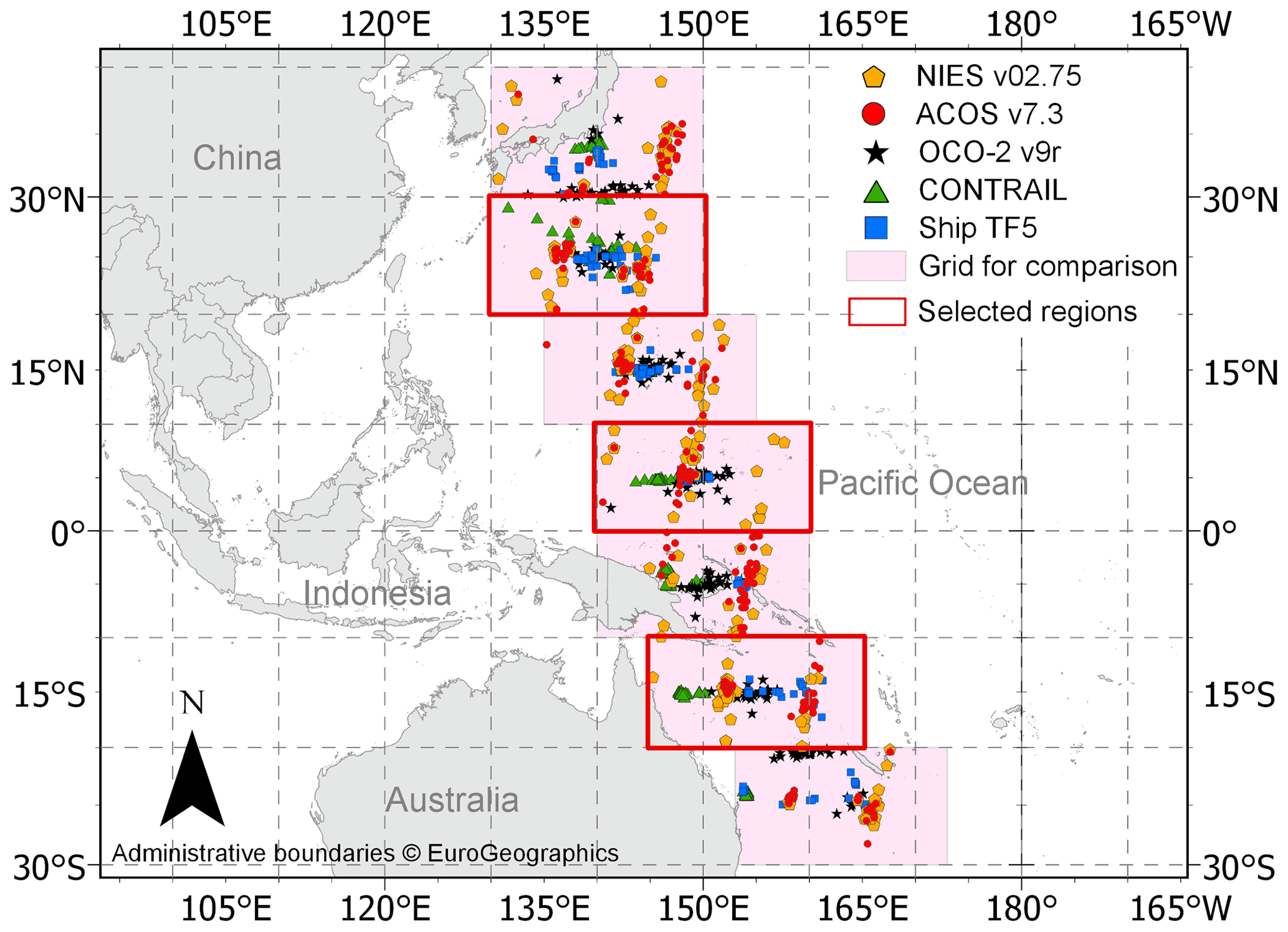
Figure 1Location of monthly averaged data of CO2 from aircraft (CONTRAIL, green triangle), ship (Trans Future 5 – TF5, blue squares), the satellite retrievals from NIES (yellow diamonds), ACOS (red circles), and OCO-2 (black stars) between 2014 and 2017. Selected regions within 10∘ latitude by 20∘ longitude boxes are shown in red frames. Administrative boundaries © EuroGeographics.
3.2 Observation-based CO2 profile construction and XCO2 calculation
Figure 2 shows how atmospheric CO2 profiles are constructed with the aid of ship and aircraft data in order to derive column-averaged mixing ratios of CO2. Ship data are extrapolated vertically to ∼ 850 hPa, which correspond to the third and fourth pressure levels of NIES and ACOS, respectively, counted from the surface. We chose this cutoff as it represents the boundary layer above sea level in which most of the rapid variation of CO2 occurs. Previous balloon and aircraft measurements by the HIPPO campaign over the tropical eastern and western Pacific showed stronger CO2 variation of about 1 to 2 ppm within the first 2 km above sea level. Above this level, the CO2 mixing ratios were rather stable or kept changing linearly up to about the tropopause height (Frankenberg et al., 2016; Inai et al., 2018). To account for that variation within the boundary layer, we added a ±2 ppm uncertainty to the CO2 estimates at ∼ 850 hPa. Aircraft data from the cruise portion of the flight, which is usually between 380 and 200 hPa, are selected. These aircraft data are extrapolated down to the lower cruising height limit at 380 hPa and at 30–40∘ N at 400 hPa. Furthermore, the aircraft data are also extrapolated upwards to the blended tropopause pressure (TROPPB).
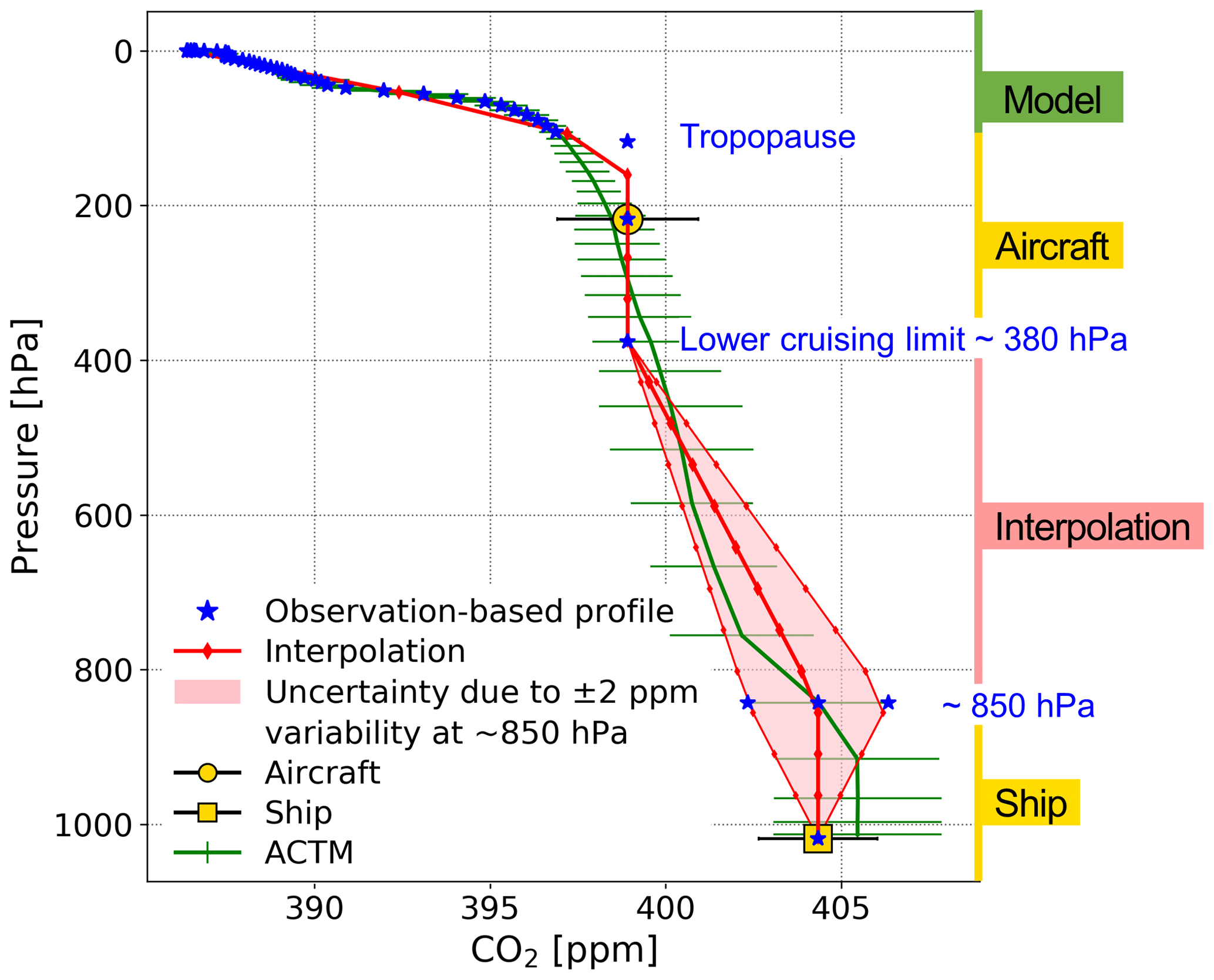
Figure 2Construction of the observation-based CO2 profile (blue) obtained by using ship (SOOP) and aircraft (CONTRAIL) data (yellow) together with the results of the ACTM (green), and the interpolation (red). The example is obtained at the latitude 20–30∘ N, March 2014.
The TROPPB is defined as a combination of a thermal tropopause and dynamic tropopause pressure (Wilcox et al., 2012). The TROPPB data are extracted from GEOS-FP (Goddard Earth Observing System – forward processing) meteorology data using the Python suite “ginput” version 1.0.6 (Laughner et al., 2021a). Ginput was developed to generate a priori vertical mixing ratios of chemical species (e.g., CO2, CO, CH4, and N2O) for the open-source TCCON retrieval algorithm, GGG2020 (Laughner et al., 2021b). The TROPPB was calculated every 3 h on the 5th, 15th, and 25th of each month for each center location of the 10∘ latitude by 20∘ longitude boxes. Between 2014 and 2017, the highest monthly variation was found at 20–30∘ N with a standard deviation ranging from 0 to 24 hPa (0.02 to 23.77 hPa) and an average standard deviation of 10 ± 5 hPa. The maximum difference of 24 hPa at the level of the TROPPB corresponds to difference in the altitude of 1 to 2 km. Assuming a straight profile between the extrapolated aircraft and ship data, we linearly interpolate in both pressure and volume mixing ratio.
Total column observations in the atmosphere consist of up to 40 % air in the stratosphere (Patra et al., 2018). To account for the stratospheric partial column, we used results of the MIROC4-ACTM (Patra et al., 2018) above the TROPPB (Fig. 2) instead of the results from ginput. First, by using the MIROC4-ACTM, our method is fully independent of TCCON, which is important for using our methodology as a complement to TCCON to evaluate satellite retrievals. Second, the MIROC4-ACTM uses realistic flux and transport simulations and is one of the best validated stratospheric models at present.
To calculate the XCO2 that the satellite would have seen given the CO2 profile constructed from in situ data, we first interpolate these profiles onto the corresponding monthly averaged pressure grid of the ACOS and NIES retrievals; then we use Eq. (15) of Connor et al. (2008):
Here, is the total column XCO2 that the satellite would report if it observed the constructed CO2 profile xm. We refer to as “observation-based XCO2” (obs. XCO2) in the following. xm is the observation-based CO2 profile (as a true profile). Extracted from the corresponding satellite retrievals, is the a priori XCO2 of OCO-2, NIES, and ACOS, respectively, hj the pressure weighting function, which is the change of atmospheric transmittance with respect to the pressure, is the column-averaging kernel, which represents the sensitivity profile to the total column amount, and xa the a priori CO2 profile. Comparison between monthly averages of the calculated obs. XCO2 using and xa from the NIES and ACOS files showed agreement within 0.1 ± 0.1 ppm. Because the ACOS retrieval provides a higher number of valid data, we used the pressure levels and parameters from ACOS as representative of the calculation. After May 2016, we use the pressure grid and parameters from NIES due to the temporal limit of the ACOS v7.3 product.
It is noted that in our approach to obtain obs. XCO2, the usage of model results above the TROPPB introduces little bias for two reasons. First, the CO2 mixing ratio at these pressure levels varies much less than that in the middle and lower troposphere since there are no significant CO2 sources and sinks in the stratosphere. Second, as mentioned earlier, the MIROC4-ACTM is among the best validated stratospheric models using high-altitude balloon-borne measurements of SF6 and CO2 age of air (Patra et al., 2018), and in the upper troposphere and lower stratosphere using CONTRAIL observations (Bisht et al., 2021). Furthermore, in a sensitivity test, we compared XCO2 derived from CO2 profiles using the MIROC4-ACTM with that where the part of the CO2 profile above the TROPPB was filled in by extrapolating the aircraft data up to 0.0128 hPa. The difference in XCO2 was only 0.2 ± 0.1 ppm on average.
4.1 Spatiotemporal variation of CO2 seen by ships, aircraft, and satellite
Figure 3a–c present the temporal variation of monthly average CO2 mixing ratios obtained by ships and aircraft in three representative latitude ranges, namely the northern midlatitudes (20–30∘ N), the Equator region (0–10∘ N), and southern latitudes (20–10∘ S). Ship and aircraft data refer to lower and upper tropospheric CO2 mixing ratios. The largest seasonal cycle of the CO2 mixing ratio is seen in the Northern Hemisphere (NH) at 20–30∘ N. Average CO2 mixing ratios of 402.9 ± 3.6 ppm and 401.2 ± 3.1 ppm in the lower and upper troposphere exceeded that from south of the Equator by 4.5 and 1.5 ppm, respectively. Maxima occur in April to May at sea level, which is approximately 1 month earlier than in the upper troposphere (May to June). Minima seen in autumn show a greater temporal variability in the lower troposphere (August to October) than at about 10 km height (September). At 20–30∘ N, the peak-to-trough amplitude of the seasonal cycles at sea level is 8.5 ± 0.9 ppm, and it is ∼ 2 ppm larger than the amplitudes in the upper troposphere (6.5 ± 0.6 ppm). Amplitudes decrease with latitude, showing similar values of about 4 ppm at the Equator. In the Southern Hemisphere (SH), the amplitudes approach 0 at sea level (Fig. 3c). In contrast, the upper troposphere shows two small peaks, one in June and one in November/December in 2014 and 2015, and additionally in April 2016. Seasonal cycles and decreasing amplitudes in the upper troposphere from north to south (7 to 4 ppm) are similar to that observed by Matsueda et al. (2008). They found a decrease from 6 ppm at 30∘ N to 3 ppm at the Equator over the same region between 2005 to 2007 using aircraft-based flask samples. At sea level, seasonal cycle amplitudes that decrease from about 8 ppm at 20–30∘ N to 3 ppm at the Equator were reported by the global sampling network of the National Oceanic and Atmospheric Administration's Climate Monitoring and Diagnostics Laboratory (NOAA/CMDL) (Conway et al., 1994). The current observed characteristics are consistent with the previous long-term studies.
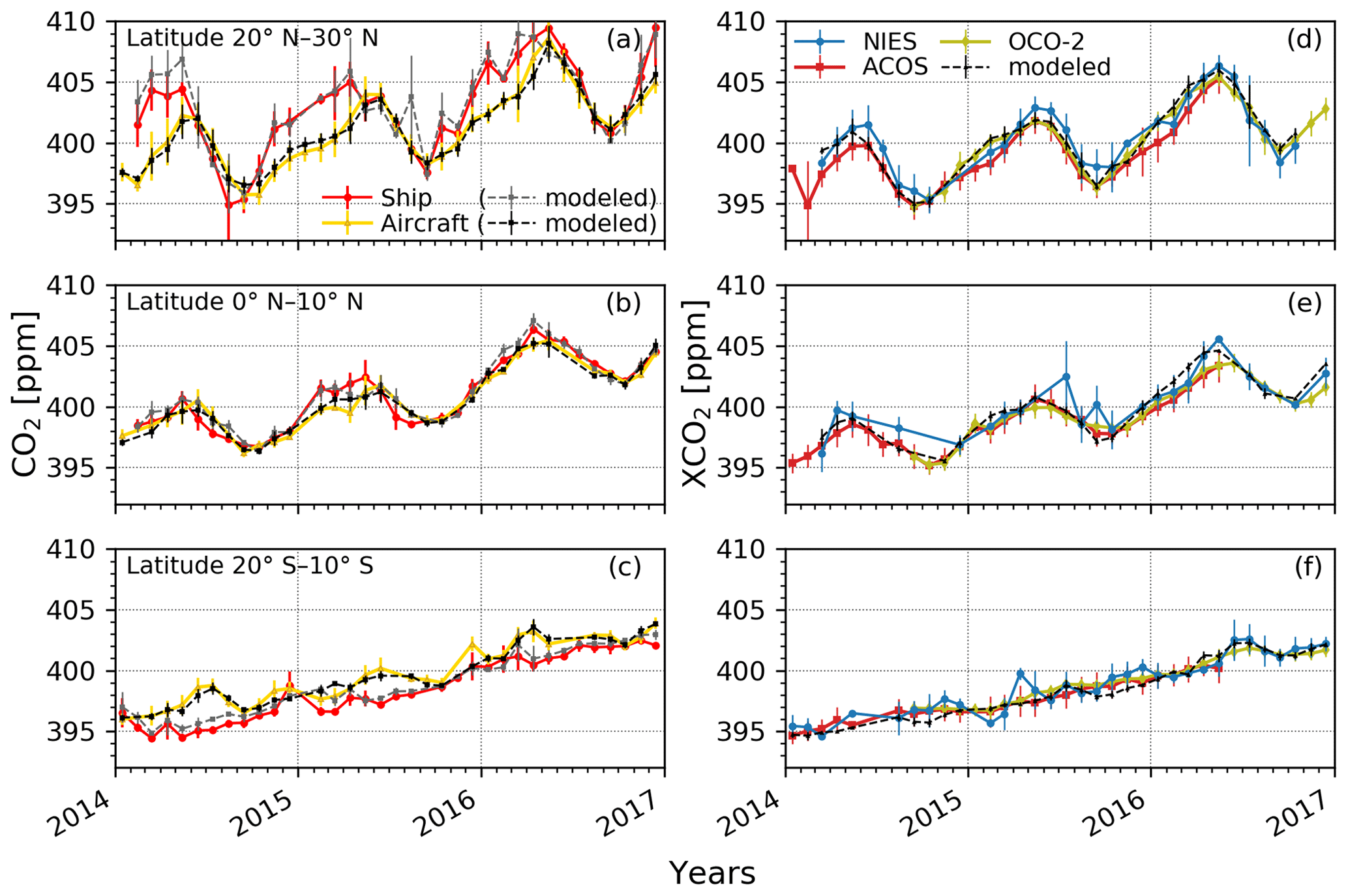
Figure 3Temporal variation of the monthly average CO2 mixing ratio obtained by ship (red) and aircraft (yellow) (a, b, c), and the column-averaged mixing ratios (XCO2) from the NIES (blue), ACOS (red), and OCO-2 (olive) (d, e, f) in three representative latitude ranges for the northern midlatitudes (a, d), the Equator region (b, e), and southern latitudes (c, f). Results of the ACTM are shown as dashed lines. Error bars represent the standard deviation of the monthly averages.
As the NH transitions from winter to spring, Fig. 3a reveals that the CO2 mixing ratio increases rapidly at the surface but only moderately at the upper troposphere, which results in a difference of up to 4 ppm. In 2014 and 2015, upper tropospheric peak values show a delay of 1 month, which is not seen in 2016, likely due to year-to-year variations. Similar observation have been made previously over the northern Pacific (Miyazaki et al., 2008; Nakazawa et al., 1991) and attributed to the response of the terrestrial carbon metabolism of the NH (China, Korea, Japan) and predominant northwesterly air-mass transport (Umezawa et al., 2018). Specifically, low net primary productivity (NPP) and leaf litter decomposition in autumn to winter is linked to a net carbon release from the terrestrial ecosystem and subsequent increase in the CO2 mixing ratio at the lower troposphere, which persists until spring. Vertical mixing mitigates the altitude-dependent CO2 gradient with a time offset of about 5 months. In spring to summer, high NPP rates substantially remove CO2 from the atmosphere. During that season, strong convection, associated with significant uplift of low-CO2 air masses, results in a well-mixed troposphere (Miyazaki et al., 2008; Nakazawa et al., 1991; Niwa et al., 2011). The flux footprint on upper tropospheric CO2 is generally much wider compared to that near the surface at all latitudes, resulting in smoother vertical gradients and smaller seasonal cycle amplitudes at higher altitudes.
Figure 3d–f present the temporal variation of column-averaged mixing ratios of CO2 (XCO2) retrieved by NIES, ACOS, and OCO-2. The number of valid bias-corrected XCO2 retrievals by NIES is less than 25 % of that by ACOS with a good quality flag. Seasonal patterns of all retrievals were similar in the NH, showing peaks in late spring/early summer (May to June), and minima in autumn (September to October). While peaks of XCO2 by NIES are higher by 1 to 3 ppm, ACOS and OCO-2 values agree within 1 ppm (Fig. 3d and e). The largest amplitudes of ACOS and OCO-2 at 20–30∘ N (5 to 6 ppm) are approximately 2 ppm smaller than those of NIES (6 to 8 ppm). Southwards, the strong seasonal cycle decreases, and it disappears in the SH, similar to observations made by in situ measurements at sea level. The NIES XCO2 product shows substantial scatter and limited valid data each month at lower latitudes, unlike ACOS and OCO-2 (Fig. 3e and f). Differences in retrieval algorithms can explain discrepancies in the XCO2 (Reuter et al., 2013), while the reduced number of data points of NIES is likely due to stricter quality filters. The results imply that seasonal variations of CO2 at lower latitudes are better represented by the ACOS/OCO-2 retrieval algorithm.
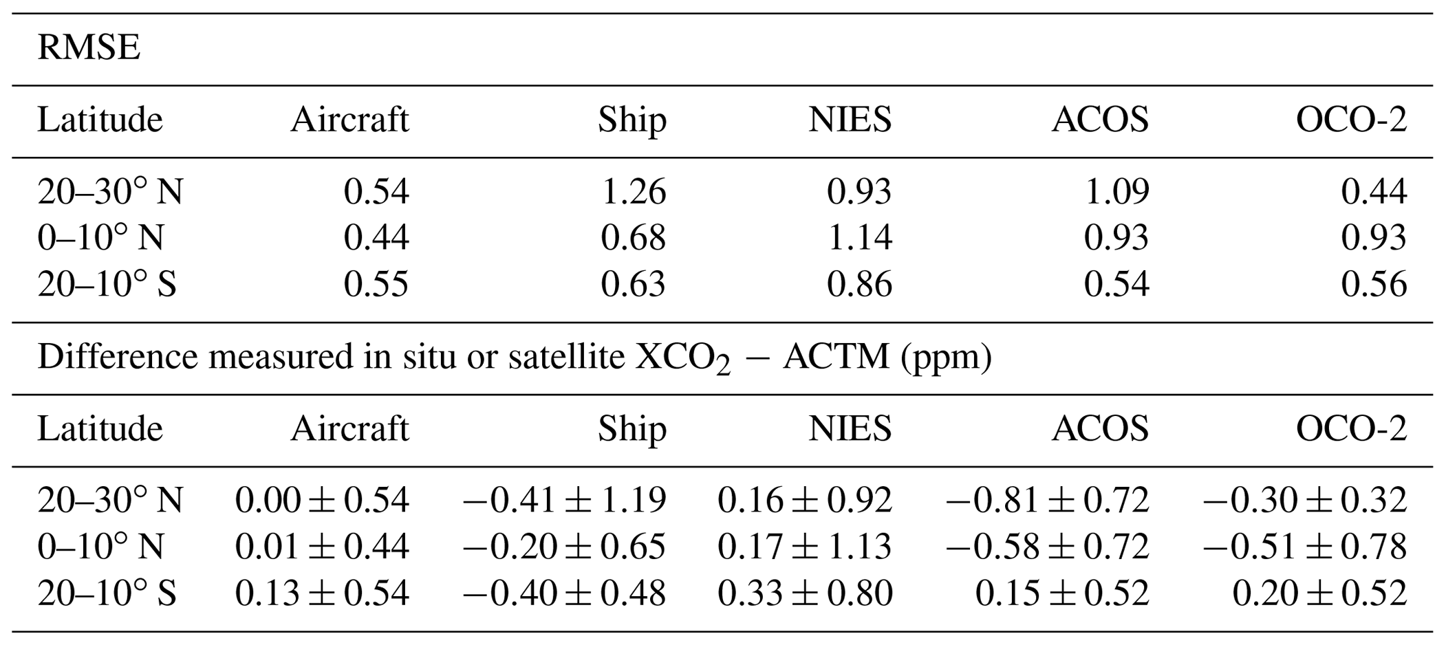
Figure 3 also presents the simulated XCO2, sea level CO2 mixing ratios, and upper troposphere CO2 mixing ratios, calculated by the MIROC4-ACTM. Best agreement is found between the model results in the upper troposphere and the aircraft observations (RMSE 0.51 ± 0.05, average difference 0.05 ± 0.06) (Table 1). The largest discrepancy with the model results occurs for the ship observations in northern midlatitudes (RMSE 1.26, difference 0.41 ± 1.19), likely due to the large gradients and variations of CO2 concentrations typically found in this latitude range at sea level. The coarse horizontal resolution of the model is not adequate to represent observations near source regions. The RMSE of the difference between satellite XCO2 and the MIROC4-ACTM ranges from 0.44 to 1.14, which may result both from the higher uncertainties of the simulations at sea level and the uncertainties in the satellite retrievals. OCO-2 v9r shows systematically higher RMSE around the Equator at 0–10∘ N, relative to the 20–30∘ N and 10–20∘ S regions.
Table 1Root-mean-square error (RMSE), and average difference and standard deviation between the retrievals from aircraft, ship, satellite and the corresponding results from the ACTM at different latitude ranges between 2014 and 2017.
4.2 Latitudinal variations of CO2 seen by ships, aircraft, and satellite
Figure 4a–c display the latitudinal distribution of the CO2 mixing ratio of ships and aircraft for three selected months in 2015, which are representative of different latitudinal CO2 gradients in the troposphere. From north towards the Equator, the negative tropospheric CO2 gradient decreases rapidly, especially in spring (March) and autumn (October) (Fig. 4a and c). Around the Equator, ship and aircraft mixing ratios agree within 0.2 ± 0.8 ppm. In the SH, the gradient is reversed, showing upper tropospheric CO2 mixing ratio to be larger by 1.4 ± 0.9 ppm, especially during NH spring to summer (Figs. 3c, 4b). Previous model studies, which included aircraft observations, explain the atmospheric CO2 characteristics south of the Equator by meridional transport processes (Miyazaki et al., 2008; Niwa et al., 2011). Our current ACTM forward simulations reveal in particular that CO2, which is strongly emitted during winter to spring (December to May) over NH land, causes a strong meridional CO2 gradient at sea level, and the CO2-rich air is transported towards the Equator (Fig. A3). In NH summer (June to August), the meridional gradient is substantially weakened due to the seasonal CO2 sink at northern midlatitudes (Figs. 4b, A3f–h). At the upper troposphere, meridional gradients are absent during autumn (September–November) (Figs. 4c, A3i–k) and gradients are weak in winter (December to February) (Fig. A3l–b) but increase towards summer due to vertical mixing of CO2-rich air from the surface at northern midlatitudes (Figs. 4a, A3c–e). Near the Equator, uplift by convection increase the CO2 mixing ratio in the middle and upper troposphere in all seasons. In the SH, strong meridional transport from the NH to the SH occurs only from late spring to early summer in the upper troposphere during which time the CO2 mixing ratio in the upper troposphere exceeds that at the sea surface (Fig. 4b). Furthermore, CO2 uptake by the southern Pacific and SH land vegetation decrease CO2 at sea level. The current in situ observations confirm the interhemispheric transport mechanism of CO2.
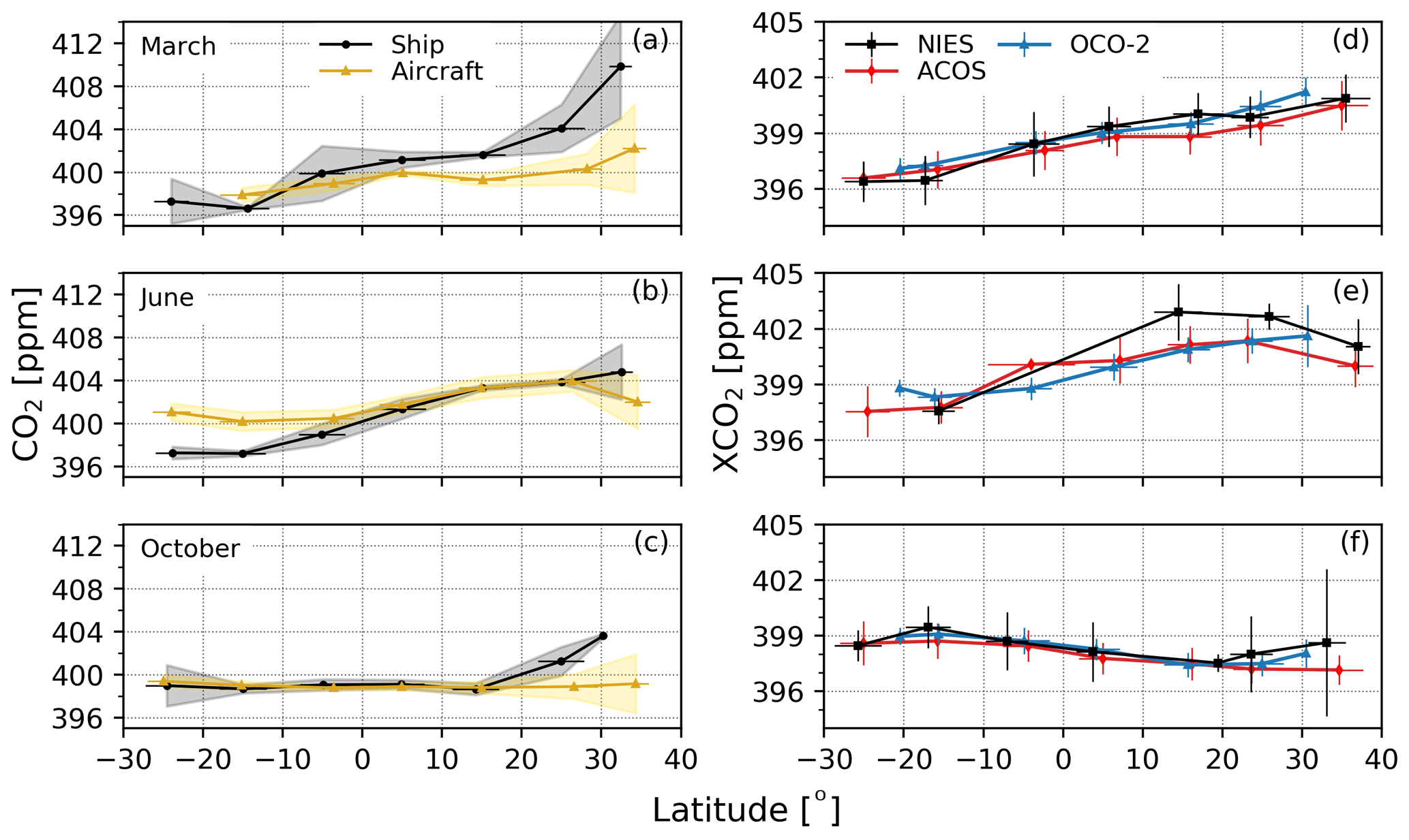
Figure 4Latitudinal distribution of the CO2 mixing ratio obtained by ship (black) and aircraft (yellow) (a, b, c) and of XCO2 obtained by NIES (black), ACOS (red), and OCO-2 (blue) (d, e, f) for three selected months in 2015, which are representative of different latitudinal CO2 gradients in the troposphere: March (a, d), June (b, e), and October (c, f). Shaded areas are the standard deviation of the monthly average CO2 mixing ratios. Error bars show the standard deviation of the monthly averaged XCO2 and of the location within each latitude box.
Figure 4d–f show the latitudinal distribution of XCO2 retrieved by NIES, ACOS, and OCO-2. In spring, maximum values appear in the NH and minima in the SH (Fig. 4d). In autumn, the locations of the maxima and minima are reversed between NH and SH (Fig. 4f). In summer (June), the maxima occur at 10–20∘ N (Fig. 4e), which is the result of substantial carbon removal by high NPP at higher latitudes (30–40∘ N) as described above. At that transition point, XCO2 of NIES exceeds that of ACOS and OCO-2 by about 2 ppm. The in situ and satellite observations reveal the complex CO2 fluxes and transport processes. The results demonstrate that measuring upper and lower tropospheric CO2 mixing ratios simultaneously is important to better understand CO2 fluxes, which is necessary to further improve atmospheric chemistry-transport models. The consistency of the satellite XCO2 with in situ observations will be evaluated by comparison with the corresponding obs. XCO2 values in the following section.
4.3 Evaluation of seasonal and interannual changes of satellite XCO2 by combined ship and aircraft observations
Figure 5a–c show the temporal variation of the satellite and obs. XCO2, and the difference between obs. and satellite XCO2 in Fig. 5d–f. The uncertainties of the obs. XCO2 dataset are estimated to be 0.62 ± 0.01 ppm on average, which is derived from the ±2 ppm variation in the observation-based CO2 profile at 2 km above sea level (Sect. 3.2).
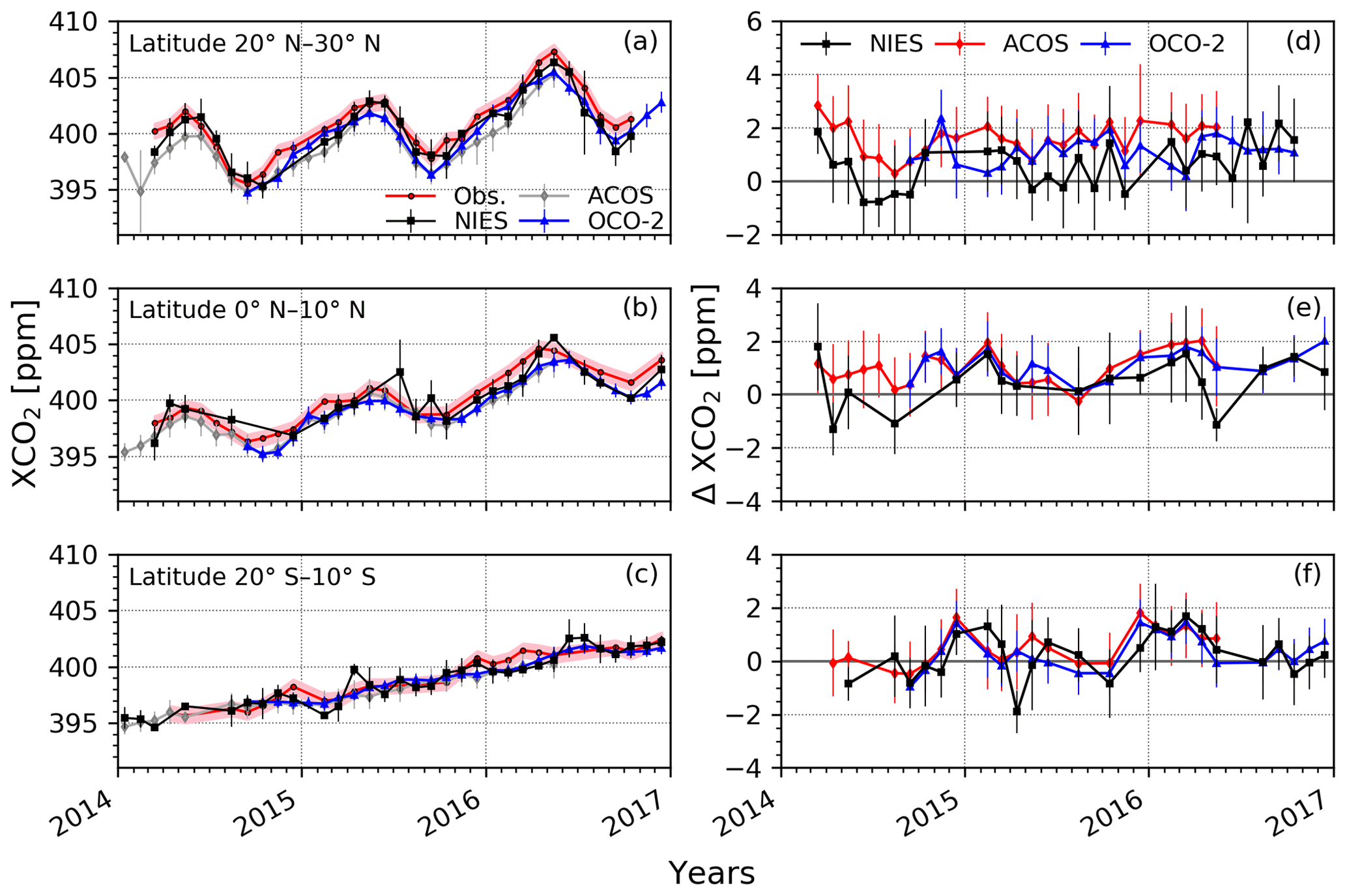
Figure 5Temporal variation of the satellite-derived XCO2 obtained by NIES (black), ACOS (gray), and OCO-2 (blue) in comparison with the obs. XCO2 (red) (a, b, c), and the difference between obs. XCO2 and NIES (black), ACOS (red), and OCO-2 (blue) (d, e, f) for three selected latitude boxes. Red-shaded areas are the uncertainty of the obs. XCO2 which was derived from the ±2 ppm variability in the observation-based CO2 profile at ∼ 850 hPa. Error bars show the standard deviation of the monthly averaged XCO2.
In all latitudes, obs. and satellite XCO2 show an overall significant positive correlation (R2: NIES = 0.84 ± 0.02, ACOS = 0.74 ± 0.08, OCO-2 = 0.82 ± 0.05) (Table 2). However, in the NH, satellite retrievals are negatively biased by up to 1.6 ± 0.6 ppm (ACOS) at 20–30∘ N (Fig. 5a and d, Table 3). The smallest average bias is found for NIES, likely due to the stricter quality filters as discussed in Sect. 4.1. While ACOS and OCO-2 show rather a systematic offset, the NIES retrieval seems to be more noisy (Fig. 5d and e, Table 3). The root-mean-square error (RMSE) of the difference between obs. XCO2 and satellite XCO2 is 1.06, 1.26, and 1.70 for NIES, OCO-2, and ACOS, respectively, and decreases by 40 % (0.56 ppm) on average between the northernmost and southernmost regions (Table 2). Agreement within 1 ppm on average is found in the SH (Fig. 5c and f). The uncertainties of the differences between obs. XCO2 and the satellite retrievals are large. However, the comparison indicates whether the results of the current satellite retrievals tend to show a systematic positive or negative offset (ACOS, OCO-2), or rather a random discrepancy. This comparison is of importance for revising the retrieval algorithm in future.
Table 2Coefficient of determination (R2) and root-mean-square error (RMSE) between obs. XCO2 and satellite XCO2 retrievals from GOSAT (NIES, ACOS) and OCO-2 at different latitude ranges between 2014 and 2017.
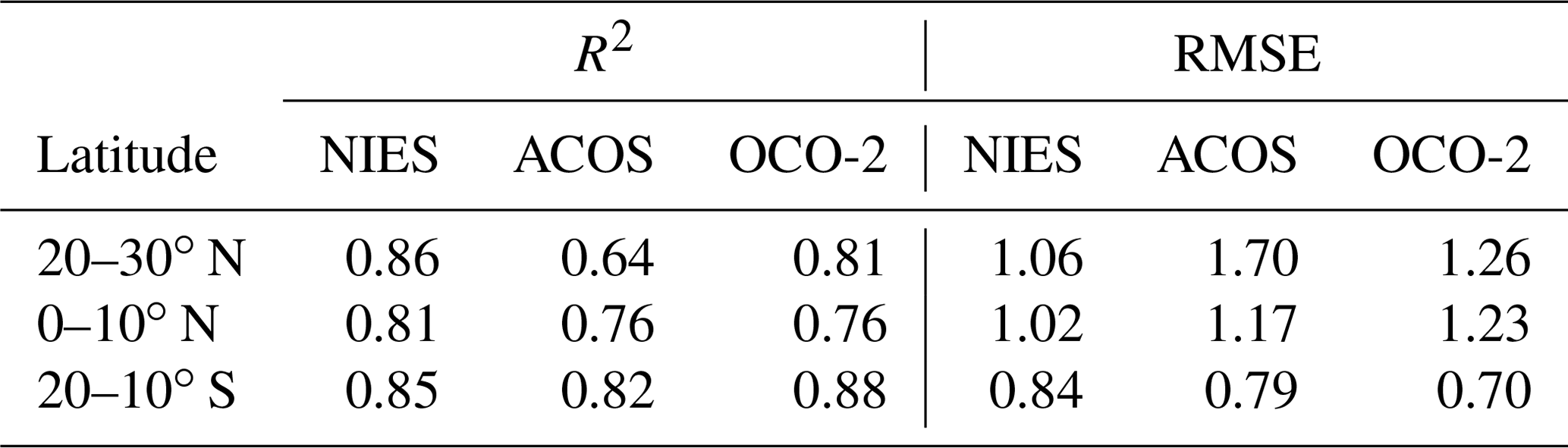
Figure 6 displays the latitudinal gradients and the gradient of the difference between obs. and satellite XCO2 for the three selected months (March, June, and October) in 2015 as described above (Sect. 4.2). It reveals that, generally, the largest differences in the NH coincide with the latitude of the monthly XCO2 maxima. Namely, this is at 30–40∘ N in spring and autumn with up to 3 ppm (between obs. XCO2 and ACOS in March) (Fig. 6a and d) and in June at 10–20∘ N with a discrepancy of up to 2 ppm (between obs. XCO2 and OCO-2) (Fig. 6b and e). The difference might be caused by uncertainties in the obs. XCO2 due to the variability of the TROPPB (Sect. 3.2). However, the uncertainty in the TROPPB results in a difference in the obs. XCO2 of only 0.03 ± 0.06 ppm on average. This leads to a total estimated error of 0.7 ppm considering the uncertainty of 0.62 ± 0.01 ppm derived from the ±2 ppm variation in the observation-based CO2 profile at 2 km above sea level (Sect. 3.2). It is known that atmospheric CO2 mixing ratios in midlatitudes are characterized by high spatiotemporal variability. Therefore, the observed discrepancies in the NH may arise from differences in sample numbers, location, and time within each month and latitude–longitude range. In particular, the largest uncertainty in the obs. XCO2 likely results from the constructed CO2 profile in the mid-troposphere, as no observational constraints are available for that part of the atmosphere, and simply a linear interpolation between the ship and aircraft data was assumed (Sect. 3.2).
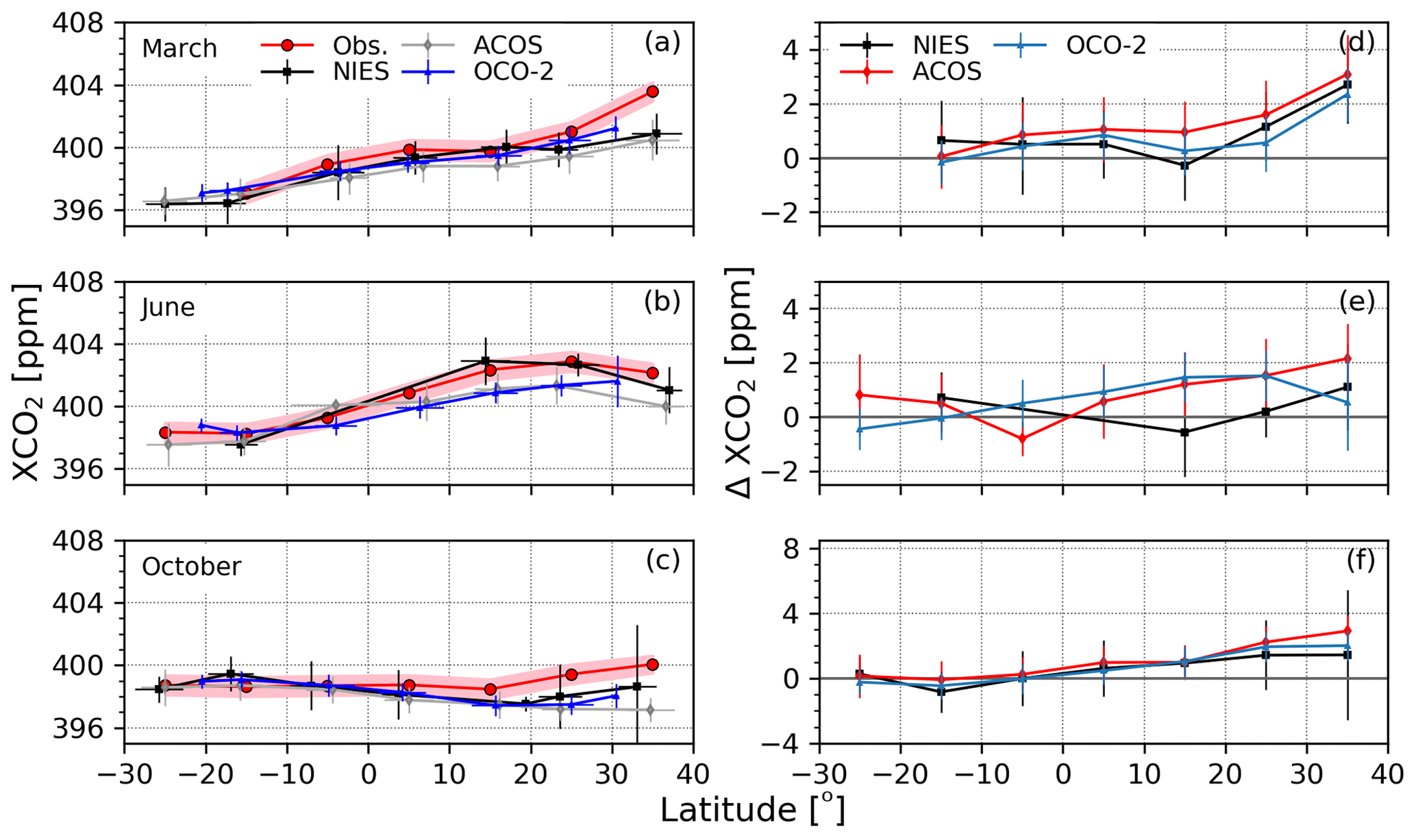
Figure 6Latitudinal gradients of obs. XCO2 (red) in comparison with the satellite XCO2 from NIES (black), ACOS (gray), and OCO-2 (blue) (a, b, c), and the difference between the obs. XCO2 and NIES (black), ACOS (red), and OCO-2 (blue) (d, e, f) for three selected months, March (a, d), June (b, e), and October (c, f), in 2015. Red-shaded areas are the uncertainty of the obs. XCO2 which was derived from the ±2 ppm variability in the observation-based CO2 profile at ∼ 850 hPa. Error bars show the standard deviation of the monthly averaged XCO2 and of the location within each latitude box.
However, Fig. 3a reveals that ship and aircraft CO2 mixing ratios are very similar in the second half of each year. Model results of the MIROC4-ACTM confirm vertically uniform CO2 profiles during that period, which lie within the uncertainty range of the observation-based profiles (Fig. A4). Niwa et al. (2011) found similar straight vertical profiles between June and September in East Asia, based on aircraft observations and model results. Furthermore, the maximum bias due to errors in the MIROC4-ACTM stratospheric CO2 profile (0.9 ppm) is smaller than the average difference of 1.2 ± 0.4 ppm between the obs. XCO2 and satellite observations of ACOS and OCO-2 between June and September (Sect. 3.2). Hence, even though no assumption was necessary at that period, the negative bias persists (Figs. 5d, 6e), which indicates that the difference between obs. and satellite XCO2 can be linked to measurement uncertainties of the satellites.
The peak values in the carbon cycle represent the turning points between predominant CO2 sources in boreal winter, and sinks in summer and therefore are important to constrain changes in the seasonal and interannual variation of the carbon cycle. Figure 5a and b reveal that maxima and minima generally agree. However, small positive phase shifts of about 1 month are occasionally observed (2014, 20–30∘ N: maximum of NIES in June; 2014, 10–20∘ N: minima of ACOS and OCO-2 in October; 2016, 10–20∘ N: maximum of OCO-2 in June). Long-term measurements (1984 to 2013) observed maxima usually in May and minima in late September in the upper troposphere of the northern West Pacific (Matsueda et al., 2008, 2015). Surface data (between 1987 and 2017) reported maxima in early May and minima in early September over the same region (World Data Centre for Greenhouse Gases (WDCGG) of the World Meteorological Organization (WMO)). The consistency with long-term studies support the correctness of the obs. XCO2, which implies that satellite XCO2 sometimes show a delayed response to CO2 changes, which might be caused by remaining uncertainties introduced by limitations in the retrieval algorithms and have not been previously identified due to the lack of validation data over the open ocean.
Table 3Average (avg.) difference and the standard deviation (SD) between obs. and satellite XCO2 from GOSAT (NIES, ACOS) and OCO-2 of each latitude range between 2014 and 2017.

To explore year-to-year changes in the increase of XCO2, the mean values of the three consecutive highest monthly averages during spring of each year are compared (Table 4). The 3-month averages around the peak values are chosen due to the limited data, although usually longer time periods are needed for that growth calculation. From 2014 to 2015, obs. and satellite XCO2 increased by 1.61 ± 0.24 ppm yr−1 on average at 20–30∘ N (Table 4, Fig. 5a). In contrast, a significant increase of 3.84 ± 0.65 ppm yr−1 is observed by obs. XCO2 from 2015 to 2016. The average increase of the mean values of all satellite retrievals is 3.39 ± 0.03 ppm yr−1. This rapid increase is also seen near the Equator, where the increase of the obs. XCO2 is significantly higher than that of ACOS and OCO-2 (two-sided t test, significance level α=0.05). Simultaneously, a larger negative bias of the satellite XCO2 in 2016 as compared to the previous years is observed (Fig. 5b and e).
The larger increase between 2015 and 2016 is likely driven by the strong El Niño in 2015. Matsueda et al. (2008) reported a mean CO2 growth rate of 1.7 to 1.8 ppm yr−1 in 1993 to 2005. However, between 1997 to 1998, they found a significantly enhanced growth rate of about 3 ppm yr−1, which they linked to a strong El Niño year (Matsueda et al., 2002, 2008). Indeed, it is well documented that the interannual variation in the growth rate of CO2 is closely linked to the El Niño–Southern Oscillation (ENSO), which affects the carbon cycle though changes in the atmospheric and ocean circulation (e.g., Bacastow, 1976; Keeling and Revelle, 1985; Kim et al., 2016; Patra et al., 2005; Wang et al., 2013; Zeng et al., 2005). Particularly, the increase of CO2 was attributed to a decrease in the NPP, increased soil respiration, and enhanced fire emissions related to low precipitation and high temperatures (Liu et al., 2017). Recent model results found that the maximum CO2 growth rate appears several months after the El Niño peak as response to the low NPP (Kim et al., 2016). In fact, the maximum increase observed in this study occurred in NH spring, after the peak of the 2015 El Niño in November/December (Fig. 5a and b).
Table 4Increase of XCO2 between peaks of consecutive years and the standard error of the difference seen by obs. and satellite XCO2 of GOSAT (NIES, ACOS) and OCO-2 between 2014 and 2017. Peak values are defined as the mean of the three consecutive highest monthly averages during spring of each year. In 2016, the mean of ACOS and that of obs. XCO2 at 0–10∘ N is based on 2 months due to limited data. “–” indicates missing data. The right column shows the average increase of all satellite means and its standard deviation.

Opposite to the strong increase, obs. XCO2 shows no increase between March and April around the Equator in 2015 (Fig. 5b). A reduction in XCO2 is seen by ACOS and OCO-2 1 month earlier (February). It has been argued that the upwelling of carbon-rich water to the surface at the Equator is suppressed in the eastern and central Pacific Ocean during El Niño (Feely et al., 2002; Keeling and Revelle, 1985), which subsequently leads to an initial negative CO2 anomaly over that region (Rayner et al., 1999). Coincident timing of the observed anomalies with different phases of the El Niño suggests that the ocean and terrestrial response to the event affect the atmospheric CO2 mixing ratio even at the study region at 140 to 160∘ E. In support of this interpretation, Chatterjee et al. (2017) found a negative anomaly in atmospheric CO2 concentrations over the so-called Niño 3.4 region (120–170∘ W) between March and July 2015 in the OCO-2 retrievals. Consequently, ACOS and OCO-2 reflect the negative anomaly of CO2 of the first phase of the El Niño, whereas in the second phase, the response of the atmospheric CO2 mixing ratio to the event is better represented by the higher growth rate of the obs. XCO2. Given the uncertainties associated with the negative CO2 anomaly observed in the study region, the result therefore suggests that, compared to satellite observations, obs. XCO2 sometimes shows a higher sensitivity to year-to-year changes in the atmospheric CO2 mixing ratio.
The current study indicates that seasonal, latitudinal, and interannual variations of atmospheric CO2 mixing ratios over the open ocean can be accurately determined by observation-based column-average CO2 mixing ratios, defined as obs. XCO2. The sensitivity of the obs. XCO2 dataset to year-to-year variations was demonstrated on the distinct ocean and terrestrial responses to the 2015–2016 El Niño event around the Equator. Namely, a stagnation in the springtime increase during the early stage of the El Niño event was linked to reduced CO2 outgassing from the ocean and a substantial increase to the later stage, reflecting the increase of CO2 emissions from the terrestrial ecosystem.
The evaluation of three different satellite retrievals (ACOS, NIES, OCO-2) by the obs. XCO2 revealed similar seasonal pattern (R2 = 0.64–0.87). However, a negative bias of 1.12 ± 0.40 ppm on average and higher difference in the NH than in the SH were attributed to measurement uncertainties of the satellites. Compared to ACOS and OCO-2, the NIES retrieval showed higher accuracy in the northern hemispherical midlatitudes. At low latitudes, NIES retrievals show substantial scatter and very few valid data points. ACOS and OCO-2 provide a more reliable analysis of carbon cycles at these latitudes. The seasonal cycle of all retrievals occasionally showed a positive phase shift of 1 month relative to the obs. XCO2 at different times of year. In some cases, the representation of year-to-year variations in atmospheric CO2 mixing ratios is more distinct in the obs. XCO2 values as compared to the satellite estimates, and therefore they are suggested to be sometimes of higher sensitivity. Hence, the result indicates that even if the retrievals complement each other, measurement uncertainties remain, which limit the accurate interpretation of spatiotemporal changes in CO2 fluxes by satellites alone. These uncertainties might be introduced by limitations in the retrieval algorithms and have not been previously identified due to the lack of validation data over the open ocean.
Advanced observations like those from GOSAT-2 and improvements in retrieval algorithms like those from ACOS version 9, and OCO-2 version 10, increase the number of valid data points at lower latitudes and reduce uncertainties. An initial comparison of the obs. XCO2 dataset with ACOS v9 revealed a decrease of the negative bias by more than 50 % on average as compared to ACOS v7.3 (Fig. A1), and the comparison with OCO-2 v10, a decrease of the average bias by more than 90 % as compared to OCO-2 v9r (Fig. A2). This example highlights the utility of the obs. XCO2 dataset as a reference for satellite-derived XCO2 estimates and to clarify the impacts of changes between different versions of retrieval algorithms.
Our study provides a short-term perspective on the great potential of the new bottom-up approach which can help us understand changes in the carbon cycle in response to global warming and interpret their contribution to atmospheric CO2 growth. We propose that a long-term XCO2 dataset based on co-located CO2 measurements by commercial ships and aircraft can augment TCCON data for validating XCO2 estimates from satellites over the open ocean. To accomplish this objective, these commercial ship and aircraft measurements should be expanded and must be sustained for the foreseeable future.
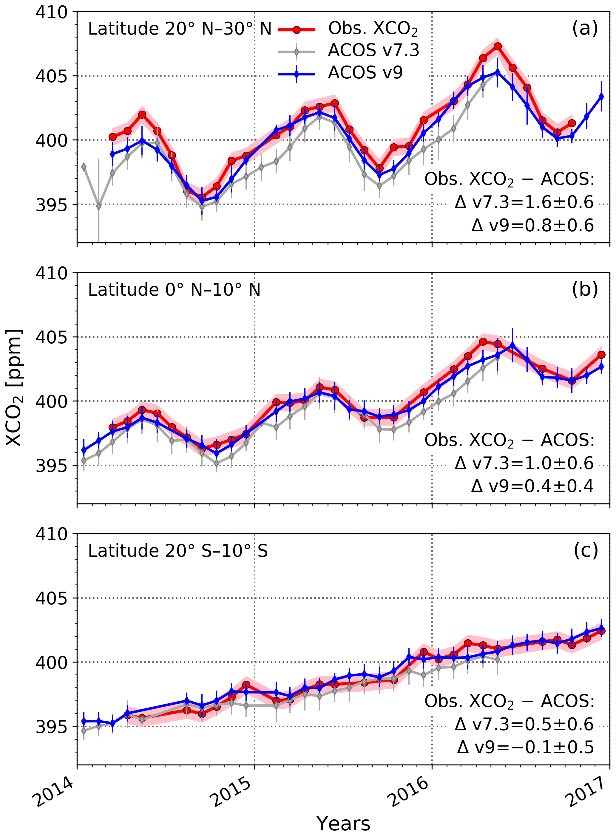
Figure A1Comparison of the temporal variation of obs. XCO2 (red) with XCO2 derived from ACOS v7.3 (gray) and ACOS v9 (blue) for three selected latitude ranges. Red-shaded areas are the uncertainty of the obs. XCO2 which was derived from the ±2 ppm variability in the observation-based CO2 profile at ∼ 850 hPa. Error bars show the standard deviation of the monthly averaged XCO2.

Figure A2Comparison of the temporal variation of obs. XCO2 (red) with XCO2 derived from OCO-2 v9r (gray) and OCO-2 v10 (blue) for three selected latitude ranges. Red-shaded areas are the uncertainty of the obs. XCO2 which was derived from the ±2 ppm variability in the observation-based CO2 profile at ∼ 850 hPa. Error bars show the standard deviation of the monthly averaged XCO2.

Figure A3Latitude–pressure distribution of the inversion of the CO2 mixing ratio at longitude 146∘ E in 2015, obtained from ACTM forward simulations.
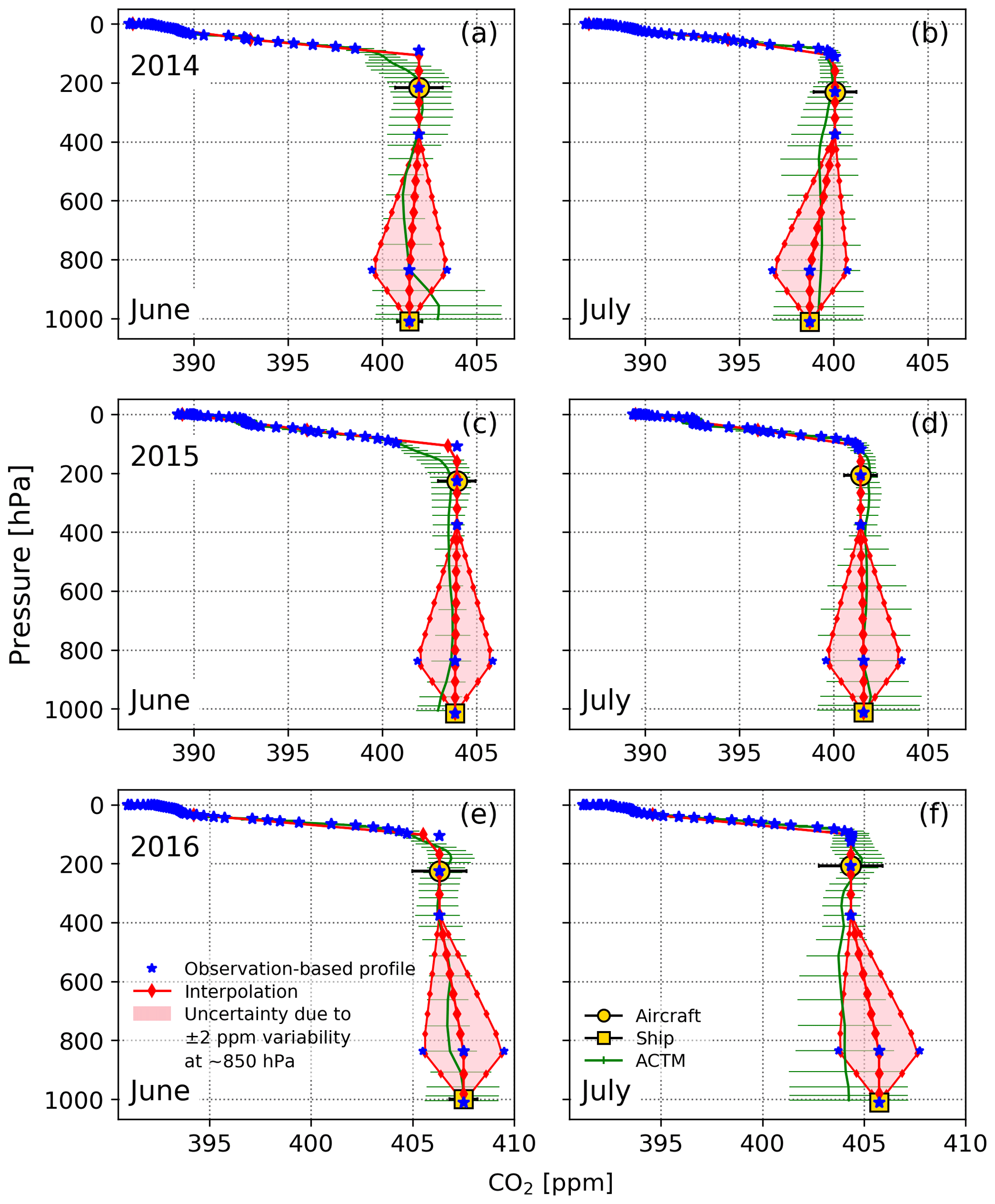
Figure A4Observation-based CO2 profiles (blue) obtained by using ship (SOOP) and aircraft (CONTRAIL) data (yellow), together with the results of the ACTM (green), and the interpolation (red) for the months June and July in 2014 (a, b), 2015 (c, d), and 2016 (e, f) at the latitude range 20–30∘ N.
The OCO-2 data presented in this paper are available from the NASA Goddard GES DISC at https://disc.gsfc.nasa.gov/datasets/OCO2_L2_Lite_FP_9r/summary (OCO-2 Science Team et al., 2018). ACOS data are available at https://disc.gsfc.nasa.gov/datasets/ACOS_L2_Lite_FP_9r/summary (OCO-2 Science Team et al., 2019) and at https://disc.gsfc.nasa.gov/datasets/ACOS_L2_Lite_FP_7.3/summary (OCO-2 Science Team et al., 2016). GOSAT data are available from the GOSAT Project website (2020) of the National Institute for Environmental Studies (NIES) at https://data2.gosat.nies.go.jp/index_en.html. SOOP data are available at http://soop.jp/ (National Institute for Environmental Studies, 2019). The CONTRAIL CME CO2 data are available on the Global Environmental Database of the Center for Global Environmental Studies of NIES (https://doi.org/10.17595/20180208.001, Machida et al., 2008). The CONTRAIL data are also available from the ObsPack data product (http://www.esrl.noaa.gov/gmd/ccgg/obspack/, last access: 26 May 2021) and the World Data Center for Greenhouse Gases (https://gaw.kishou.go.jp/, last access: 26 May 2021).
The supplement related to this article is available online at: https://doi.org/10.5194/acp-21-8255-2021-supplement.
The study was designed by HT. Data analyses were made by AM, and extensive discussions were made by AM, HT, TS, TM, PKP, JL, and DC. The paper was written, edited, and proofed by all the authors.
The authors declare that they have no conflict of interest.
We are grateful to Naveen Chandra (NIES) for providing CO2 inversion fluxes that are used for simulating atmospheric concentration by ACTM. We also would like to thank the anonymous reviewers for the valuable comments and suggestions for improving the paper.
The authors acknowledge the satellite data infrastructure for providing access to the GOSAT NIES, GOSAT ACOS, and OCO-2 data used in this study. This research is a contribution to the Research Announcement on GOSAT series joint research, titled “Combined cargo-ship and passenger aircraft observations-based validation of GOSAT-2 GHG observations over the open oceans”, and to the Greenhouse Gas Initiative of the Atmospheric Composition Virtual Constellation (AC-VC) of the Committee on Earth Observation Satellites (CEOS). We thank the WDCGG (World Data Centre for Greenhouse Gases) for providing CO2 reference data of the Pacific Ocean from the NOAA GMD Carbon Cycle Cooperative Global Air Sampling Network, 1968–2018 (principal investigators include Ed Dlugokencky (NOAA)). Part of this work was conducted at the Jet Propulsion Laboratory, California Institute of Technology, under contract to the National Aeronautics and Space Administration. Government sponsorship is acknowledged.
This research has been supported by the Global Environmental Research Coordination System from the Ministry of the Environment (Japan) (grant nos. E1851, E1253, E1652, E1151, E1951, E1451, E1751, and E1432) and the Environmental Research and Technology Development Fund (ERTDF) from the Ministry of the Environment (Japan) (grant no. 2-1803. JPMEERF20182003).
This paper was edited by Anita Ganesan and reviewed by two anonymous referees.
Bacastow, R. B.: Modulation of atmospheric carbon dioxide by the Southern Oscillation, Nature, 261, 116–118, https://doi.org/10.1038/261116a0, 1976.
Baker, D. F., Bösch, H., Doney, S. C., O'Brien, D., and Schimel, D. S.: Carbon source/sink information provided by column CO2 measurements from the Orbiting Carbon Observatory, Atmos. Chem. Phys., 10, 4145–4165, https://doi.org/10.5194/acp-10-4145-2010, 2010.
Basu, S., Guerlet, S., Butz, A., Houweling, S., Hasekamp, O., Aben, I., Krummel, P., Steele, P., Langenfelds, R., Torn, M., Biraud, S., Stephens, B., Andrews, A., and Worthy, D.: Global CO2 fluxes estimated from GOSAT retrievals of total column CO2, Atmos. Chem. Phys., 13, 8695–8717, https://doi.org/10.5194/acp-13-8695-2013, 2013.
Bisht, J. S. H., Machida, T., Chandra, N., Tsuboi, K., Patra, P. K., Umezawa, T., Niwa, Y., Sawa, Y., Morimoto, S., Nakazawa, T., Saitoh, N., and Takigawa, M.: Seasonal Variations of SF6, CO2, CH4, and N2O in the UT/LS Region due to Emissions, Transport, and Chemistry, J. Geophys. Res.-Atmos., 126, 1–18, https://doi.org/10.1029/2020JD033541, 2021.
Canadell, J. G., Ciais, P., Gurney, K., Le Quéré, C., Piao, S., Raupach, M. R., and Sabine, C. L.: An International Effort to Quantify Regional Carbon Fluxes, Eos T. Am. Geophys. Un., 92, 81–82, https://doi.org/10.1029/2011EO100001, 2011.
Chatterjee, A., Gierach, M. M., Sutton, A. J., Feely, R. A., Crisp, D., Eldering, A., Gunson, M. R., O'Dell, C. W., Stephens, B. B., and Schimel, D. S.: Influence of El Niño on atmospheric CO2 over the tropical Pacific Ocean: Findings from NASA's OCO-2 mission, Science, 358, eaam5776, https://doi.org/10.1126/science.aam5776, 2017.
Chevallier, F., Ciais, P., Conway, T. J., Aalto, T., Anderson, B. E., Bousquet, P., Brunke, E. G., Ciattaglia, L., Esaki, Y., Fröhlich, M., Gomez, A., Gomez-Pelaez, A. J., Haszpra, L., Krummel, P. B., Langenfelds, R. L., Leuenberger, M., Machida, T., Maignan, F., Matsueda, H., Morguí, J. A., Mukai, H., Nakazawa, T., Peylin, P., Ramonet, M., Rivier, L., Sawa, Y., Schmidt, M., Steele, L. P., Vay, S. A., Vermeulen, A. T., Wofsy, S., and Worthy, D.: CO2 surface fluxes at grid point scale estimated from a global 21 year reanalysis of atmospheric measurements, J. Geophys. Res., 115, D21307, https://doi.org/10.1029/2010JD013887, 2010.
Chevallier, F., Deutscher, N. M., Conway, T. J., Ciais, P., Ciattaglia, L., Dohe, S., Fröhlich, M., Gomez-Pelaez, A. J., Griffith, D., Hase, F., Haszpra, L., Krummel, P., Kyrö, E., Labuschagne, C., Langenfelds, R., Machida, T., Maignan, F., Matsueda, H., Morino, I., Notholt, J., Ramonet, M., Sawa, Y., Schmidt, M., Sherlock, V., Steele, P., Strong, K., Sussmann, R., Wennberg, P., Wofsy, S., Worthy, D., Wunch, D., and Zimnoch, M.: Global CO2 fluxes inferred from surface air-sample measurements and from TCCON retrievals of the CO2 total column, Geophys. Res. Lett., 38, L24810, https://doi.org/10.1029/2011GL049899, 2011.
Connor, B. J., Boesch, H., Toon, G., Sen, B., Miller, C., and Crisp, D.: Orbiting Carbon Observatory: Inverse method and prospective error analysis, J. Geophys. Res.-Atmos., 113, 1–14, https://doi.org/10.1029/2006JD008336, 2008.
Conway, T. J., Tans, P. P., Waterman, L. S., Thoning, K. W., Kitzis, D. R., Masarie, K. A., and Zhang, N.: Evidence for interannual variability of the carbon cycle from the National Oceanic and Atmospheric Administration/Climate Monitoring and Diagnostics Laboratory Global Air Sampling Network, J. Geophys. Res., 99, 22831, https://doi.org/10.1029/94JD01951, 1994.
Crisp, D., Fisher, B. M., O'Dell, C., Frankenberg, C., Basilio, R., Bösch, H., Brown, L. R., Castano, R., Connor, B., Deutscher, N. M., Eldering, A., Griffith, D., Gunson, M., Kuze, A., Mandrake, L., McDuffie, J., Messerschmidt, J., Miller, C. E., Morino, I., Natraj, V., Notholt, J., O'Brien, D. M., Oyafuso, F., Polonsky, I., Robinson, J., Salawitch, R., Sherlock, V., Smyth, M., Suto, H., Taylor, T. E., Thompson, D. R., Wennberg, P. O., Wunch, D., and Yung, Y. L.: The ACOS CO2 retrieval algorithm – Part II: Global XCO2 data characterization, Atmos. Meas. Tech., 5, 687–707, https://doi.org/10.5194/amt-5-687-2012, 2012.
Crisp, D., Pollock, H. R., Rosenberg, R., Chapsky, L., Lee, R. A. M., Oyafuso, F. A., Frankenberg, C., O'Dell, C. W., Bruegge, C. J., Doran, G. B., Eldering, A., Fisher, B. M., Fu, D., Gunson, M. R., Mandrake, L., Osterman, G. B., Schwandner, F. M., Sun, K., Taylor, T. E., Wennberg, P. O., and Wunch, D.: The on-orbit performance of the Orbiting Carbon Observatory-2 (OCO-2) instrument and its radiometrically calibrated products, Atmos. Meas. Tech., 10, 59–81, https://doi.org/10.5194/amt-10-59-2017, 2017.
Crowell, S., Baker, D., Schuh, A., Basu, S., Jacobson, A. R., Chevallier, F., Liu, J., Deng, F., Feng, L., McKain, K., Chatterjee, A., Miller, J. B., Stephens, B. B., Eldering, A., Crisp, D., Schimel, D., Nassar, R., O'Dell, C. W., Oda, T., Sweeney, C., Palmer, P. I., and Jones, D. B. A.: The 2015–2016 carbon cycle as seen from OCO-2 and the global in situ network, Atmos. Chem. Phys., 19, 9797–9831, https://doi.org/10.5194/acp-19-9797-2019, 2019.
Dlugokencky, E. and Tans, P.: Trends in Atmospheric Carbon Dioxide, NOAA/GML, available at: http://www.esrl.noaa.gov/gmd/ccgg/trends/, last access: 7 January 2021.
Feely, R. A., Boutin, J., Cosca, C. E., Dandonneau, Y., Etcheto, J., Inoue, H. Y., Ishii, M., Quéré, C. Le, Mackey, D. J., McPhaden, M., Metzl, N., Poisson, A., and Wanninkhof, R.: Seasonal and interannual variability of CO2 in the equatorial Pacific, Deep-Sea Res. Pt. II, 49, 2443–2469, https://doi.org/10.1016/S0967-0645(02)00044-9, 2002.
Frankenberg, C., Kulawik, S. S., Wofsy, S. C., Chevallier, F., Daube, B., Kort, E. A., O'Dell, C., Olsen, E. T., and Osterman, G.: Using airborne HIAPER Pole-to-Pole Observations (HIPPO) to evaluate model and remote sensing estimates of atmospheric carbon dioxide, Atmos. Chem. Phys., 16, 7867–7878, https://doi.org/10.5194/acp-16-7867-2016, 2016.
Friedlingstein, P., Jones, M. W., O'Sullivan, M., Andrew, R. M., Hauck, J., Peters, G. P., Peters, W., Pongratz, J., Sitch, S., Le Quéré, C., Bakker, D. C. E., Canadell, J. G., Ciais, P., Jackson, R. B., Anthoni, P., Barbero, L., Bastos, A., Bastrikov, V., Becker, M., Bopp, L., Buitenhuis, E., Chandra, N., Chevallier, F., Chini, L. P., Currie, K. I., Feely, R. A., Gehlen, M., Gilfillan, D., Gkritzalis, T., Goll, D. S., Gruber, N., Gutekunst, S., Harris, I., Haverd, V., Houghton, R. A., Hurtt, G., Ilyina, T., Jain, A. K., Joetzjer, E., Kaplan, J. O., Kato, E., Klein Goldewijk, K., Korsbakken, J. I., Landschützer, P., Lauvset, S. K., Lefèvre, N., Lenton, A., Lienert, S., Lombardozzi, D., Marland, G., McGuire, P. C., Melton, J. R., Metzl, N., Munro, D. R., Nabel, J. E. M. S., Nakaoka, S.-I., Neill, C., Omar, A. M., Ono, T., Peregon, A., Pierrot, D., Poulter, B., Rehder, G., Resplandy, L., Robertson, E., Rödenbeck, C., Séférian, R., Schwinger, J., Smith, N., Tans, P. P., Tian, H., Tilbrook, B., Tubiello, F. N., van der Werf, G. R., Wiltshire, A. J., and Zaehle, S.: Global Carbon Budget 2019, Earth Syst. Sci. Data, 11, 1783–1838, https://doi.org/10.5194/essd-11-1783-2019, 2019.
GOSAT Project website: GOSAT Bias-corrected FTS SWIR Level 2 CO2 Product (V02.75), available at: https://data2.gosat.nies.go.jp/index_en.html, release note available at: https://data2.gosat.nies.go.jp/doc/documents/ReleaseNote_FTSSWIRL2_BiasCorrCO2_V02.75_en.pdf, last access: 28 April 2020.
Hakkarainen, J., Ialongo, I., Maksyutov, S., and Crisp, D.: Analysis of Four Years of Global XCO2 Anomalies as Seen by Orbiting Carbon Observatory-2, Remote Sens., 11, 850, https://doi.org/10.3390/rs11070850, 2019.
Inai, Y., Aoki, S., Honda, H., Furutani, H., Matsumi, Y., Ouchi, M., Sugawara, S., Hasebe, F., Uematsu, M., and Fujiwara, M.: Balloon-borne tropospheric CO2 observations over the equatorial eastern and western Pacific, Atmos. Environ., 184, 24–36, https://doi.org/10.1016/j.atmosenv.2018.04.016, 2018.
Inoue, M., Morino, I., Uchino, O., Miyamoto, Y., Yoshida, Y., Yokota, T., Machida, T., Sawa, Y., Matsueda, H., Sweeney, C., Tans, P. P., Andrews, A. E., Biraud, S. C., Tanaka, T., Kawakami, S., and Patra, P. K.: Validation of XCO2 derived from SWIR spectra of GOSAT TANSO-FTS with aircraft measurement data, Atmos. Chem. Phys., 13, 9771–9788, https://doi.org/10.5194/acp-13-9771-2013, 2013.
Intergovernmental Panel on Climate Change (IPCC): Climate Change 2013 – The Physical Science Basis, edited by Intergovernmental Panel on Climate Change, Cambridge University Press, Cambridge, 2013.
Keeling, C. D. and Revelle, R.: Effects of El Nino/Southern Oscillation on the Atmospheric Content of Carbon Dioxide, Meteoritics, 20, 437–450, 1985.
Kim, J. S., Kug, J. S., Yoon, J. H., and Jeong, S. J.: Increased atmospheric CO2 growth rate during El Niño driven by reduced terrestrial productivity in the CMIP5 ESMs, J. Climate, 29, 8783–8805, https://doi.org/10.1175/JCLI-D-14-00672.1, 2016.
Kobayashi, S., Ota, Y., Harada, Y., Ebita, A., Moriya, M., Onoda, H., Onogi, K., Kamahori, H., Kobayashi, C., Endo, H., Miyaoka, K., and Takahashi, K.: The JRA-55 Reanalysis: General Specifications and Basic Characteristics, J. Meteorol. Soc. Jpn. Ser. II, 93, 5–48, https://doi.org/10.2151/jmsj.2015-001, 2015.
Kulawik, S. S., Crowell, S., Baker, D., Liu, J., McKain, K., Sweeney, C., Biraud, S. C., Wofsy, S., O'Dell, C. W., Wennberg, P. O., Wunch, D., Roehl, C. M., Deutscher, N. M., Kiel, M., Griffith, D. W. T., Velazco, V. A., Notholt, J., Warneke, T., Petri, C., De Mazière, M., Sha, M. K., Sussmann, R., Rettinger, M., Pollard, D. F., Morino, I., Uchino, O., Hase, F., Feist, D. G., Roche, S., Strong, K., Kivi, R., Iraci, L., Shiomi, K., Dubey, M. K., Sepulveda, E., Rodriguez, O. E. G., Té, Y., Jeseck, P., Heikkinen, P., Dlugokencky, E. J., Gunson, M. R., Eldering, A., Crisp, D., Fisher, B., and Osterman, G. B.: Characterization of OCO-2 and ACOS-GOSAT biases and errors for CO2 flux estimates, Atmos. Meas. Tech. Discuss. [preprint], https://doi.org/10.5194/amt-2019-257, 2019.
Kuze, A., Suto, H., Nakajima, M., and Hamazaki, T.: Thermal and near infrared sensor for carbon observation Fourier-transform spectrometer on the Greenhouse Gases Observing Satellite for greenhouse gases monitoring, Appl. Optics, 48, 6716, https://doi.org/10.1364/AO.48.006716, 2009.
Laughner, J., Andrews, A., Roche, S., Kiel, M., and Toon, G.: ginput v1.0.7b: GGG2020 prior profile software, [Computer software], CaltechDATA, https://doi.org/10.22002/D1.1944, 2021a.
Laughner, J. L., Kiel, M., Toon, G., Andrews, A., Roche, S., Wunch, D., and Wennberg, P. O.: Revised formulation of the TCCON priors for GGG2020, in preparation, 2021b.
Liu, J., Bowman, K. W., Schimel, D. S., Parazoo, N. C., Jiang, Z., Lee, M., Bloom, A. A., Wunch, D., Frankenberg, C., Sun, Y., O'Dell, C. W., Gurney, K. R., Menemenlis, D., Gierach, M., Crisp, D., and Eldering, A.: Contrasting carbon cycle responses of the tropical continents to the 2015–2016 El Niño, Science, 358, https://doi.org/10.1126/science.aam5690, 2017.
Machida, T., Matsueda, H., Sawa, Y., Nakagawa, Y., Hirotani, K., Kondo, N., Goto, K., Nakazawa, T., Ishikawa, K., and Ogawa, T.: Worldwide measurements of atmospheric CO2 and other trace gas species using commercial airlines, J. Atmos. Ocean. Technol., 25, 1744–1754, https://doi.org/10.1175/2008JTECHA1082.1, 2008.
Machida, T., Ishijima, K., Niwa, Y., Tsuboi, K., Sawa, Y., and Matsueda, H.: Atmospheric CO2 mole fraction data of CONTRAIL-CME, NIES, https://doi.org/10.17595/20180208.001, 2018.
Matsueda, H., Inoue, H. Y., and Ishii, M.: Aircraft observation of carbon dioxide at 8–13 km altitude over the Western Pacific from 1993 to 1999, Tellus B, 54, 1–21, https://doi.org/10.1034/j.1600-0889.2002.00304.x, 2002.
Matsueda, H., Machida, T., Sawa, Y., Nakagawa, Y., Hirotani, K., Ikeda, H., Kondo, N., and Goto, K.: Evaluation of atmospheric CO2 measurements from new flask air sampling of JAL airliner observations, Pap. Meteorol. Geophys., 59, 1–17, https://doi.org/10.2467/mripapers.59.1, 2008.
Matsueda, H., Machida, T., Sawa, Y., and Niwa, Y.: Long-term change of CO2 latitudinal distribution in the upper troposphere, Geophys. Res. Lett., 42, 2508–2514, https://doi.org/10.1002/2014GL062768, 2015.
Miller, C. E., Crisp, D., DeCola, P. L., Olsen, S. C., Randerson, J. T., Michalak, A. M., Alkhaled, A., Rayner, P., Jacob, D. J., Suntharalingam, P., Jones, D. B. A., Denning, A. S., Nicholls, M. E., Doney, S. C., Pawson, S., Boesch, H., Connor, B. J., Fung, I. Y., O'Brien, D., Salawitch, R. J., Sander, S. P., Sen, B., Tans, P., Toon, G. C., Wennberg, P. O., Wofsy, S. C., Yung, Y. L., and Law, R. M.: Precision requirements for space-based data, J. Geophys. Res.-Atmos., 112, 1–19, https://doi.org/10.1029/2006JD007659, 2007.
Miyazaki, K., Patra, P. K., Takigawa, M., Iwasaki, T., and Nakazawa, T.: Global-scale transport of carbon dioxide in the troposphere, J. Geophys. Res.-Atmos., 113, 1–21, https://doi.org/10.1029/2007JD009557, 2008.
Morino, I., Tsutsumi, Y., Uchino, O., Ohyama, H., Thi Ngoc Trieu, T., Frey, M. M., Yoshida, Y., Matsunaga, T., Kamei, A., Saito, M., and Noda, H. M.: Status of GOSAT and GOSAT-2 FTS SWIR L2 Product Validation, in: The 16th International Workshop on Greenhouse Gas Measurement from Space, 2–5, 2020.
Nakajima, M., Suto, H., Yotsumoto, K., Shiomi, K., and Hirabayashi, T.: Fourier transform spectrometer on GOSAT and GOSAT-2, in International Conference on Space Optics – ICSO 2014, vol. 10563, edited by: Cugny, B., Sodnik, Z., and Karafolas, N., SPIE, 2 pp., 2017.
Nakazawa, T., Miyashita, K., Aoki, S., and Tanaka, M.: Temporal and spatial variations of upper tropospheric and lower stratospheric carbon dioxide, Tellus B, 43, 106–117, https://doi.org/10.1034/j.1600-0889.1991.t01-1-00005.x, 1991.
National Institute for Environmental Studies: NIES volunteer Observing Ship Program dataset, available at: http://soop.jp/, last access: 26 September 2019.
Niwa, Y., Patra, P. K., Sawa, Y., Machida, T., Matsueda, H., Belikov, D., Maki, T., Ikegami, M., Imasu, R., Maksyutov, S., Oda, T., Satoh, M., and Takigawa, M.: Three-dimensional variations of atmospheric CO2: aircraft measurements and multi-transport model simulations, Atmos. Chem. Phys., 11, 13359–13375, https://doi.org/10.5194/acp-11-13359-2011, 2011.
OCO-2 Science Team, Gunson, M., and Eldering, A.: ACOS GOSAT/TANSO-FTS Level 2 bias-corrected XCO2 and other select fields from the full-physics retrieval aggregated as daily files V7.3, Greenbelt, MD, USA, Goddard Earth Sciences Data and Information Services Center (GES DISC), available at: https://disc.gsfc.nasa.gov/datacollection/ACOS_L2_Lite_FP_7.3.html (last access: 16 April 2020), 2016.
OCO-2 Science Team, Gunson, M., and Eldering, A.: OCO-2 Level 2 bias-corrected XCO2 and other select fields from the full-physics retrieval aggregated as daily files, Retrospective processing V9r, Greenbelt, MD, USA, Goddard Earth Sciences Data and Information Services Center (GES DISC), https://doi.org/10.5067/W8QGIYNKS3JC, 2018.
OCO-2 Science Team, Gunson, M., and Eldering, A.: ACOS GOSAT/TANSO-FTS Level 2 bias-corrected XCO2 and other select fields from the full-physics retrieval aggregated as daily files V9r, Greenbelt, MD, USA, Goddard Earth Sciences Data and Information Services Center (GES DISC), https://doi.org/10.5067/VWSABTO7ZII4, 2019.
O'Dell, C. W., Connor, B., Bösch, H., O'Brien, D., Frankenberg, C., Castano, R., Christi, M., Eldering, D., Fisher, B., Gunson, M., McDuffie, J., Miller, C. E., Natraj, V., Oyafuso, F., Polonsky, I., Smyth, M., Taylor, T., Toon, G. C., Wennberg, P. O., and Wunch, D.: The ACOS CO2 retrieval algorithm – Part 1: Description and validation against synthetic observations, Atmos. Meas. Tech., 5, 99–121, https://doi.org/10.5194/amt-5-99-2012, 2012.
O'Dell, C. W., Eldering, A., Wennberg, P. O., Crisp, D., Gunson, M. R., Fisher, B., Frankenberg, C., Kiel, M., Lindqvist, H., Mandrake, L., Merrelli, A., Natraj, V., Nelson, R. R., Osterman, G. B., Payne, V. H., Taylor, T. E., Wunch, D., Drouin, B. J., Oyafuso, F., Chang, A., McDuffie, J., Smyth, M., Baker, D. F., Basu, S., Chevallier, F., Crowell, S. M. R., Feng, L., Palmer, P. I., Dubey, M., García, O. E., Griffith, D. W. T., Hase, F., Iraci, L. T., Kivi, R., Morino, I., Notholt, J., Ohyama, H., Petri, C., Roehl, C. M., Sha, M. K., Strong, K., Sussmann, R., Te, Y., Uchino, O., and Velazco, V. A.: Improved retrievals of carbon dioxide from Orbiting Carbon Observatory-2 with the version 8 ACOS algorithm, Atmos. Meas. Tech., 11, 6539–6576, https://doi.org/10.5194/amt-11-6539-2018, 2018.
Patra, P. K., Maksyutov, S., Sasano, Y., Nakajima, H., Inoue, G., and Nakazawa, T.: An evaluation of CO2 observations with Solar Occultation FTS for Inclined-Orbit Satellite sensor for surface source inversion, J. Geophys. Res.-Atmos., 108, 4759, https://doi.org/10.1029/2003JD003661, 2003.
Patra, P. K., Ishizawa, M., Maksyutov, S., Nakazawa, T., and Inoue, G.: Role of biomass burning and climate anomalies for land-atmosphere carbon fluxes based on inverse modeling of atmospheric CO2, Global Biogeochem. Cy., 19, 1–10, https://doi.org/10.1029/2004GB002258, 2005.
Patra, P. K., Takigawa, M., Watanabe, S., Chandra, N., Ishijima, K., and Yamashita, Y.: Improved chemical tracer simulation by MIROC4.0-based atmospheric chemistry-transport model (MIROC4-ACTM), Sci. Online Lett. Atmos., 14, 91–96, https://doi.org/10.2151/SOLA.2018-016, 2018.
Rayner, P. J., Law, R. M., and Dargaville, R.: The relationship between tropical CO2 fluxes and the El Niño-Southern Oscillation, Geophys. Res. Lett., 26, 493–496, https://doi.org/10.1029/1999GL900008, 1999.
Reuter, M., Bösch, H., Bovensmann, H., Bril, A., Buchwitz, M., Butz, A., Burrows, J. P., O'Dell, C. W., Guerlet, S., Hasekamp, O., Heymann, J., Kikuchi, N., Oshchepkov, S., Parker, R., Pfeifer, S., Schneising, O., Yokota, T., and Yoshida, Y.: A joint effort to deliver satellite retrieved atmospheric CO2 concentrations for surface flux inversions: the ensemble median algorithm EMMA, Atmos. Chem. Phys., 13, 1771–1780, https://doi.org/10.5194/acp-13-1771-2013, 2013.
Sawa, Y., Machida, T., and Matsueda, H.: Aircraft observation of the seasonal variation in the transport of CO2 in the upper atmosphere, J. Geophys. Res.-Atmos., 117, D05305, https://doi.org/10.1029/2011JD016933, 2012.
Umezawa, T., Matsueda, H., Sawa, Y., Niwa, Y., Machida, T., and Zhou, L.: Seasonal evaluation of tropospheric CO2 over the Asia-Pacific region observed by the CONTRAIL commercial airliner measurements, Atmos. Chem. Phys., 18, 14851–14866, https://doi.org/10.5194/acp-18-14851-2018, 2018.
Velazco, V. A., Morino, I., Uchino, O., Hori, A., Kiel, M., Bukosa, B., Deutscher, N. M., Sakai, T., Nagai, T., Bagtasa, G., Izumi, T., Yoshida, Y., and Griffith, D. W. T.: TCCON Philippines: First measurement results, satellite data and model comparisons in Southeast Asia, Remote Sens., 9, 1–18, https://doi.org/10.3390/rs9121228, 2017.
Wang, W., Ciais, P., Nemani, R. R., Canadell, J. G., Piao, S., Sitch, S., White, M. A., Hashimoto, H., Milesi, C., and Myneni, R. B.: Variations in atmospheric CO2 growth rates coupled with tropical temperature (Proceedings of the National Academy of Sciences of the United States of America (2013) 110, 32 (13061-13066) https://doi.org/10.1073/pnas.1219683110), P. Natl. Acad. Sci. USA, 110, 15163, https://doi.org/10.1073/pnas.1314920110, 2013.
Wilcox, L. J., Hoskins, B. J., and Shine, K. P.: A global blended tropopause based on ERA data. Part I: Climatology, Q. J. Roy. Meteor. Soc., 138, 561–575, https://doi.org/10.1002/qj.951, 2012.
Wofsy, S. C.: HIAPER Pole-to-Pole Observations (HIPPO): fine-grained, global-scale measurements of climatically important atmospheric gases and aerosols, Philos. T. R. Soc. A., 369, 2073–2086, https://doi.org/10.1098/rsta.2010.0313, 2011.
Wofsy, S. C., Afshar, S., Allen, H. M., Apel, E., Asher, E. C., Barletta, B., Bent, J., Bian, H., Biggs, B. C., Blake, D. R., Blake, N., Bourgois, I., Brock, C. A., Brune, W. H., Budney, J. W., Bui, T. P., Butler, A., Campuzano-Jost, P., Chang, C. S., Chin, M., Commane, R., Correa, G., Crounse, J. D., Cullis, P. D., Daube, B. C., Day, D. A., Dean-Day, J. M., Dibb, J. E., Digangi, J. P., Diskin, G. S., Dollner, M., Elkins, J. W., Erdesz, F., Fiore, A. M., Flynn, C. M., Froyd, K., Gesler, D. W., Hall, S. R., Hanisco, T. F., Hannun, R. A., Hills, A. J., Hintsa, E. J., Hoffmann, A., Hornbrook, R. S., Huey, L. G., Hughes, S., Jimenez, J. L., Johnson, B. J., Katich, J. M., Keeling, R., Kim, M. J., Kupc, A., Lait, L. R., Lamarque, J.-F., Liu, H. B., McKain, K., Mclaughlin, R. J., Meinardi, S., Miller, D. O., Montzka, S. A., Moore, F. L., Morgan, E. J., Murphy, D. M., Murray, L. T., Nault, B. A., Neuman, J. A., Newman, P. A., Nicely, J. M., Pan, X., Paplawsky, W., Peischl, J., Prather, M. J., Price, D. J., Ray, E., Reeves, J. M., Richardson, M., Rollins, A. W., Rosenlof, K. H., Ryerson, T. B., Scheuer, E., Schill, G. P., Schroder, J. C., Schwarz, J. P., St.Clair, J. M., Steenrod, S. D., Stephens, B. B., Strode, S. A., Sweeney, C., Tanner, D., Teng, A. P., Thames, A. B., Thompson, C. R., Ullmann, K., Veres, P. R., Vizenor, N., Wagner, N. L., Watt, A., Weber, R., Weinzierl, B., Wennberg, P., Williamson, C. J., Wilson, J. C., Wolfe, G. M., Woods, C. T., and Zeng, L. H.: ATom: Merged Atmospheric Chemistry, Trace Gases, and Aerosols, ORNL DAAC, Oak Ridge, Tennessee, USA, https://doi.org/10.3334/ORNLDAAC/1581, 2018.
Wunch, D., Toon, G. C., Blavier, J.-F. L., Washenfelder, R. A., Notholt, J., Connor, B. J., Griffith, D. W. T., Sherlock, V., and Wennberg, P. O.: The Total Carbon Column Observing Network, Philos. T. R. Soc. A, 369, 2087–2112, https://doi.org/10.1098/rsta.2010.0240, 2011.
Yamagishi, H., Tohjima, Y., Mukai, H., Nojiri, Y., Miyazaki, C., and Katsumata, K.: Observation of atmospheric oxygen/nitrogen ratio aboard a cargo ship using gas chromatography/thermal conductivity detector, J. Geophys. Res.-Atmos., 117, D04309, https://doi.org/10.1029/2011JD016939, 2012.
Yoshida, Y., Ota, Y., Eguchi, N., Kikuchi, N., Nobuta, K., Tran, H., Morino, I., and Yokota, T.: Retrieval algorithm for CO2 and CH4 column abundances from short-wavelength infrared spectral observations by the Greenhouse gases observing satellite, Atmos. Meas. Tech., 4, 717–734, https://doi.org/10.5194/amt-4-717-2011, 2011.
Yoshida, Y., Kikuchi, N., Morino, I., Uchino, O., Oshchepkov, S., Bril, A., Saeki, T., Schutgens, N., Toon, G. C., Wunch, D., Roehl, C. M., Wennberg, P. O., Griffith, D. W. T., Deutscher, N. M., Warneke, T., Notholt, J., Robinson, J., Sherlock, V., Connor, B., Rettinger, M., Sussmann, R., Ahonen, P., Heikkinen, P., Kyrö, E., Mendonca, J., Strong, K., Hase, F., Dohe, S., and Yokota, T.: Improvement of the retrieval algorithm for GOSAT SWIR XCO2 and XCH4 and their validation using TCCON data, Atmos. Meas. Tech., 6, 1533–1547, https://doi.org/10.5194/amt-6-1533-2013, 2013.
Zeng, N., Mariotti, A., and Wetzel, P.: Terrestrial mechanisms of interannual CO2 variability, Global Biogeochem. Cy., 19, 1–15, https://doi.org/10.1029/2004GB002273, 2005.