the Creative Commons Attribution 4.0 License.
the Creative Commons Attribution 4.0 License.
 | 10 May 2021
Smoke-charged vortices in the stratosphere generated by wildfires and their behaviour in both hemispheres: comparing Australia 2020 to Canada 2017
Hugo Lestrelin
Aurélien Podglajen
Mikail Salihoglu
The two most intense wildfires of the last decade that took place in Canada in 2017 and Australia in 2019–2020 were followed by large injections of smoke into the stratosphere due to pyro-convection. After the Australian event, Khaykin et al. (2020) and Kablick et al. (2020) discovered that part of this smoke self-organized as anticyclonic confined vortices that rose in the mid-latitude stratosphere up to 35 km. Based on Cloud-Aerosol Lidar with Orthogonal Polarization (CALIOP) observations and the ERA5 reanalysis, this new study analyses the Canadian case and finds, similarly, that a large plume had penetrated the stratosphere by 12–13 August 2017 and then became trapped within a mesoscale anticyclonic structure that travelled across the Atlantic. It then broke into three offspring that could be followed until mid-October, performing three round-the-world journeys and rising up to 23 km. We analyse the dynamical structure of the vortices produced by these two wildfires and demonstrate how the assimilation of the real temperature and ozone data from instruments measuring the signature of the vortices explains the appearance and maintenance of the vortices in the constructed dynamical fields. We propose that these vortices can be seen as bubbles of small, almost vanishing, potential vorticity and smoke carried vertically across the stratification from the troposphere inside the middle stratosphere by their internal heating, against the descending flux of the Brewer–Dobson circulation.
- Article
(14651 KB) - Full-text XML
-
Supplement
(35602 KB) - BibTeX
- EndNote


A spectacular consequence of large summer wildfires in mid-latitude forests is the generation of pyro-cumulonimbus (PyroCb) that can reach the lower stratosphere during extreme events (Fromm et al., 2010). The combustion products and accompanying tropospheric compounds (e.g. organic and black carbon, smoke aerosols, condensed water, carbon monoxide, and low ozone) that are lifted to the stratosphere can survive several months and be transported over considerable distances (Fromm et al., 2010; Yu et al., 2019; Kloss et al., 2019; Bourassa et al., 2019), filling the mid-latitude band and sometimes reaching the tropics (Kloss et al., 2019). As black carbon is highly absorptive of the incoming solar radiation, the resulting heating produces buoyancy (de Laat et al., 2012; Ditas et al., 2018) and an additional lift of the undiluted parts of the plume by several kilometres in the stratosphere (Khaykin et al., 2018; Yu et al., 2019). This effect enhances the dispersion and, by increasing the altitude, ensures a longer lifetime in the stratosphere (Yu et al., 2019), enhancing the amplitude of the radiative effect on climate that has been estimated to be comparable to moderate volcanic eruptions (Peterson et al., 2018; Khaykin et al., 2020).
The magnitude of Australian wildfires of the 2019–2020 summer season exceeded all previously known events (Khaykin et al., 2020). A striking discovery was the observation that a part of the stratospheric smoke plumes self-organized as anticyclonic vortices that persisted for between 1 and 3 months (Kablick et al., 2020; Khaykin et al., 2020; Allen et al., 2020); the most intense smoke plume, nicknamed “Koobor” hereafter following an aboriginal legend, rose up to 35 km (Khaykin et al., 2020) – an altitude not reached by tropospheric aerosols since the Pinatubo eruption. Khaykin et al. (2020) conjectured that aerosol heating was essential in maintaining the structure and providing the lift. In turn, the vortex created a confinement that preserved the embedded smoke cloud from being rapidly diluted within the environment.
Investigating the occurrence of such vortices after previous wildfires, in particular over the last 15 years during which the required satellite instruments are available, is a natural extension of the work of Khaykin et al. (2020). As the strongest recorded wildfire of the last decade is the 2017 Canadian event that took place in British Columbia (Hanes et al., 2019), this work revisits this case, which has already been documented in several studies (Khaykin et al., 2018; Ansmann et al., 2018; Peterson et al., 2018; Yu et al., 2019; Kloss et al., 2019; Baars et al., 2019; Torres et al., 2020). In particular, a stratospheric rise of up to 30 K d−1 in potential temperature was diagnosed based on satellite observations by Khaykin et al. (2018), and a compact smoke cloud at 19 km over the Haute-Provence Observatory, southern France, on 29 August 2017 was also reported in the same study. Another goal of this work is to complement Khaykin et al. (2020) by expanding their diagnostics and interpretations on the 2020 case.
This paper is structured as follows: Sect. 2 describes the data and methods used in this work; Sect. 3 describes the new vortices found after the 2017 Canadian fire and their evolution, including a detailed discussion of previous results; Sect. 4 describes the structure of the vortices based on the 2017 Canadian case and the 2020 Australian case; and Sect, 5 offers conclusions.
2.1 Satellite data from CALIOP
Launched in April 2006, the Cloud-Aerosol Lidar and Infrared Path Satellite Observation (CALIPSO) mission (Winker et al., 2010) hosts the Cloud-Aerosol Lidar with Orthogonal Polarization (CALIOP) onboard instrument – a two-wavelength polarization lidar that performs global profiling of aerosols and clouds in the troposphere and lower stratosphere. We used the total attenuated 532 nm backscatter Level 1 (L1) product in the latest available version, V4.10 (Powell et al., 2009). The nominal along-track horizontal and vertical resolutions respectively are 1 km and 60 m between 8.5 and 20.1 km and 1.667 km and 180 m between 20.1 and 30.1 km. The L1 product oversamples the layers above 8.5 km with a uniform horizontal resolution of 333 m. We computed the scattering ratio by dividing the total attenuated backscatter by the calculated molecular backscatter, following Vernier et al. (2009) and Hostetler et al. (2006), and using the meteorological metadata provided with the L1 product. To reduce the noise, a horizontal median filter with a 40 km width (121 pixels) was applied to the data. In order to separate clouds from aerosols, we also used the Level 2 (L2) total scattering aerosol coefficient at 532 nm which is available at a 5 km resolution. Both daytime and night-time measurements were used. As the daytime measurements are noisier, they can only be used when the aerosol signal is strong enough, mainly during the first few weeks following the release of the plume.
As in Khaykin et al. (2020), CALIOP inspection was the first step in identifying the potential vortices. The L1 sections were systematically screened from 12 August to 15 October 2017, and those that contained isolated compact patterns above 11 km and were identified as aerosols by the L2 product were selected. The location and size of the retained patches were then determined by visually matching a rectangular box to the observation, as illustrated in Fig. A1 in the Appendix. It is usually very easy to see the boundaries of the retained patches. In the next stage, the patches were associated with the vortices detected as described in the following, and further inspection rejected cases that corresponded to tails left behind by vortices (less than 20 % of those retained in the first stage).
Due to increased solar activity, CALIOP operations were suspended between 5 and 14 September. This has been an obstacle to establishing continuity based on CALIOP observations alone, but the tracking of the vortices filled that gap as described below.
2.2 Meteorological data
2.2.1 Reanalysis
To track the stratospheric wildfire vortices and diagnose their dynamical structure, we used the ERA5 reanalysis (Hersbach et al., 2020), which is the last-generation global atmospheric reanalysis of the European Centre for Medium-Range Weather Forecast (ECMWF). Khaykin et al. (2020) used the ECMWF operational analysis and forecast instead; however, both are based on the ECMWF Integrated Forecast System (IFS). In ERA5, the native horizontal resolution of the IFS model is about 31 km, and it has 137 levels in the vertical with spacing that varies from less than 400 m at 15 km to about 900 m at 35 km within the relevant altitude range of this study. We used an extracted version of ERA5 with 1∘ resolution in latitude and longitude, at full vertical resolution and 3-hourly resolution. This choice was dictated by practical considerations in addition to the fact that this grid is able to describe synoptic-scale features and that vortices do not travel across more than a few grid points in 3 h.
Khaykin et al. (2020) used temperature, ozone and vorticity to investigate the structure of the vortices. In this study, we also used potential vorticity (PV). PV is a Lagrangian invariant for inviscid and adiabatic flows (Ertel, 1942); furthermore, it provides a compact and complete picture of the balanced part of the flow (Hoskins et al., 1985). An interesting property of ERA5 is that its dynamical core preserves PV much better than previous reanalyses (Hoffmann et al., 2019). Although the ERA5 potential vorticity can be directly retrieved from the ECMWF archive on a given set of potential temperature levels, we instead recalculated it from the retrieved vorticity, temperature and total horizontal wind fields on model levels, in order to benefit from the full vertical resolution offered by ERA5. For that purpose, we used the definition of PV for the primitive equations in spherical coordinates and model hybrid vertical coordinate η, which is given by
where a is the radius of the Earth, λ is the longitude, ϕ is the latitude, g is the free-fall acceleration, ζη is the model level vertical component of the vorticity, f is the Coriolis parameter, (u,v) is the horizontal velocity, p is the pressure and θ is the potential temperature. The gradients are estimated using centred differences on the retrieved longitude–latitude–η grid. See Eqs. (3.1.4) of Andrews et al. (1987) for an analogous formula in barometric altitude coordinate.
While the formulation of PV in Eq. (1) is the most commonly used, it bears the disadvantage of a large background vertical gradient, which proves inconvenient to track and characterize structures along their ascent. To overcome this issue, we used the alternative formulation of Lait (1994), discussed by Müller and Günther (2003):
where P is the Ertel PV, ϵ=4 in the Australian case and in the Canadian case, and θ0=420 K. Compared with P, Π is still an adiabatic invariant and exhibits a reduced vertical gradient; thus, the vortices, characterized by anticyclonic Π anomalies, can be unambiguously distinguished during their ascent. In each of the two cases, the value of ϵ is chosen to nearly cancel the background vertical gradient of Π, and it depends on the large-scale vertical temperature profile characterized by larger (more positive) in the Australian case than in Canadian case (see Müller and Günther, 2003, for a discussion regarding the choice of ϵ).
2.2.2 Assimilation increment
ERA5 is constrained by observations over repeated 12 h assimilation cycles. Over each cycle, the assimilation increment is defined as the difference between the new analysis and the first guess provided as a final stage of a free forecast run of the model, initialized from the previous analysis 12 h before. This definition can be applied to any of the basic variables of the model or to derived quantities like potential vorticity. In ERA5, the assimilation increments can be calculated on each day at 06:00 and 18:00 UTC. In order to diagnose how the observations are forcing the vortices, we calculated the assimilation increments of temperature, vorticity, potential vorticity and ozone. Temperature and ozone determine the radiances that are measured by space-borne instruments and are also directly accessible from in situ instruments. On the contrary, potential vorticity cannot be directly retrieved from any instrument and is indirectly constrained (see below). These three parameters are updated by the assimilation system in order to reduce the difference between observed quantities (typically radiances but also deviations of the GPS signal path) and simulated quantities (radiances that a satellite flying “above the model” would see). It is tempting to see the temperature assimilation increment as an additional heating, but this is incorrect. The increment is calculated from an adjusted state, resulting from the iterations of the assimilation, in which both temperature and motion respond to the forcing from the observations. As wind observations are much sparser than temperature observations, one would expect that analysis winds, and related quantities like potential vorticity, are more poorly constrained and, therefore, less accurate than analysis temperatures. While this statement is true to a large extent in the tropics, the temperature and wind fields are related through thermal wind balance in the mid-latitudes. This equilibrium is enforced by the assimilation system which filters out the transient modes that deviate from it. Hence, thanks to this miracle of assimilation, assimilating the temperature signal of the vortex is sufficient to reconstruct the whole thermal and dynamical field associated with the balanced structure (McIntyre, 2015).
It should be noted here that neither the ECMWF operational analysis nor ERA5 assimilate aerosol observations. The smoke plumes are totally absent from the IFS, where stratospheric aerosols are only accounted for by the mean climatological distribution during the periods of investigation, and it is only their dynamical vortical signature which is introduced in the model as described above.
2.2.3 Vortex tracking approach
Once we caught the first occurrence of an isolated bubble of aerosols with CALIOP, we searched the ERA5 data for the occurrence of a corresponding vortex that showed up as an isolated pattern in the Π and ozone maps. While Khaykin et al. (2020) used only relative vorticity to track the vortices for convenience, we used both Π defined from Eq. (2) and the ozone anomaly defined as the deviation with respect to the zonal mean at the same latitude and altitude. Tracking was carried out every 6 h by following a local extremum within a box of usually 12∘ in longitude, 5∘ in latitude and a range of at least 30 K of potential temperature in the vertical. Once a vortex was caught, the box was moved forward in time to the step n+1 according to the vortex motion between steps n−1 and n. In very few instances, the tracking was guided by reducing the size of the box. In particular, this was needed at the formation of a vortex, or during a breaking event, when it split into two parts, or in the final stage when one of the methods lost the track before the other.

Figure 1Selection of along-track sections of the CALIOP scattering ratio profiles during the first observation period until 4 September 2017. Panels (a–d) show sections of bubble O at four times. Panels (e–h) show four sections of bubble A after its separation from bubble O. Panels (i–l) show two sections of bubble B1 after its separation from bubble O (i, j) and two views of bubble B2 that continues the track of bubble O after 1 September 2017 (k, l). In each panel, the black and red crosses show the orbital plane projection of the corresponding vortex centre according to the Lait PV Π and ozone tracking in ERA5 data respectively. For each panel, the longitude indicated in the title is that of the CALIPSO orbit at the centre of the bubble.
3.1 General description
Although the 2017 Canadian fire started in June (Hanes et al., 2019), it was not until 12 August to early on 13 August that the fire reached an intensity such that a large PyroCb developed and reached the lower stratosphere, leaving a smoke plume that could be followed by satellite sensors (Khaykin et al., 2018; Peterson et al., 2018; Torres et al., 2020). From the inspection of the scattering ratio along CALIPSO orbits, we found our first distinctly isolated smoke bubble on 16 August at 09:38 UTC and 12.6 km altitude over the north of Canada (63∘ N and 102∘ W), where the tropopause altitude was 11 km. Two days after the first evidence of the presence of smoke in the stratosphere (Peterson et al., 2018; Torres et al., 2020). In the following days and until the CALIOP interruption on 4 September, we could track this cloud, labelled as bubble O, and its offspring almost every day. Figure 1 shows several typical patterns during that period.
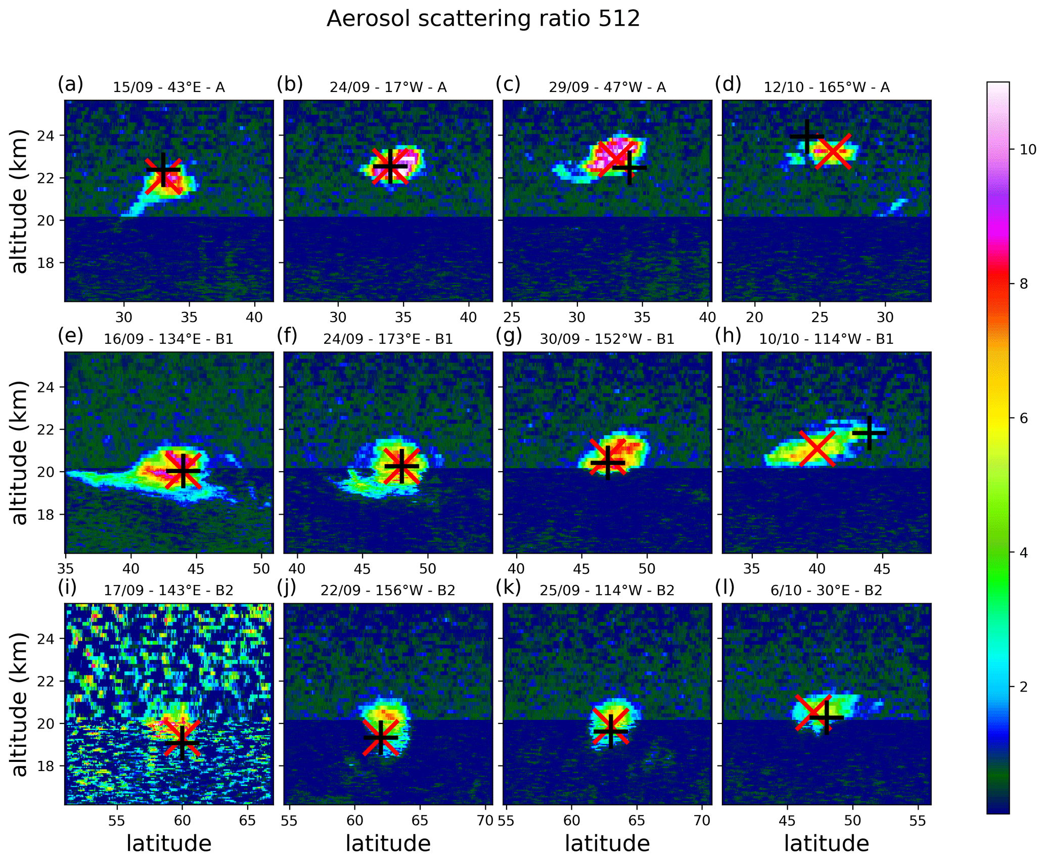
Figure 2Same as Fig. 1 but during the second observation period after 15 September 2017, showing four sections of bubbles A (a–d), B1 (e–h) and B2 (i–l).
As indicated by the longitudes in Fig. 1, bubble O moved eastward across the Atlantic. During the early days, it was captured each day by at most two CALIPSO orbits (one day orbit and one night orbit), with the adjacent orbits only showing filamentary non-compact structures that could be easily distinguished. The bubble rose rapidly reaching 18 km by 25 August (i.e. an ascent rate larger than 0.5 km d−1). One surprising feature is that once it had reached the European coast by 27 August, several bubbles could be tracked on multiple close orbits or even, exceptionally, on the same orbit. As we shall see in the following, this corresponds to the splitting of bubble O into several offspring that we label as A, B1 and B2 for which several views are shown in Fig. 1. Another issue came soon after as CALIOP operations were suspended for the period from 5 to 14 September due to increased solar activity. When CALIOP observations resumed after 14 September, the A, B1 and B2 bubbles that were now located at 20 km or above could be found again, over central Asia for A and over the Pacific for B1 and B2, and they were followed during their subsequent journey until mid-October. Figure 2 shows a selection of views during that period.
3.2 Early evolution
The smoke bubbles were attributed to vortices based on the ERA5 reanalysis which were available throughout their life cycles. Starting on 14 August, a kernel of almost zero PV and low ozone could be found at 72∘ N, 115∘ W and an altitude of 12 km just above the tropopause. In the following days, this anomaly developed vertically and connected with the bubble O location as identified from CALIOP (see animation in Sect. S2 of the Supplement). On 17 August, as it crossed Hudson Bay, it exhibited a well-developed intrusion that reached 14 km in the PV longitudinal and latitudinal section. As seen in the animation, this intrusion, while still rising, was subsequently stretched by the vertical shear and split into an upper and lower part by 19 August: the upper part was isolated in the stratosphere at about 15 km, whereas the lower part near the tropopause was further stretched and disappeared. The upper part, which was associated with bubble O, was tracked in the ERA5 ozone and PV fields and from CALIOP until the end of August (Fig. S1 in the Supplement). As it crossed the Atlantic, it became trapped inside a trough on 20 August and then travelled with it until it reached the European coast. Due to the wind shear prevailing in the associated jet, vortex O elongated in latitude across the isentropes (see the animation) until it became split into the three parts, A, B1 and B2, over western Europe, as described in the next section.
This early stage is also described in great detail by Torres et al. (2020). This previous study shows that the whole smoke cloud is shaped like a V, on 20 August, by its passage in the trough, resulting in a double maximum tilted pattern in the section by CALIOP. This pattern is recovered in the ERA5 PV pattern (freeze the animation in Sect. S2 of the Supplement on the same date), and our tracking actually follows the highest of the two maxima.
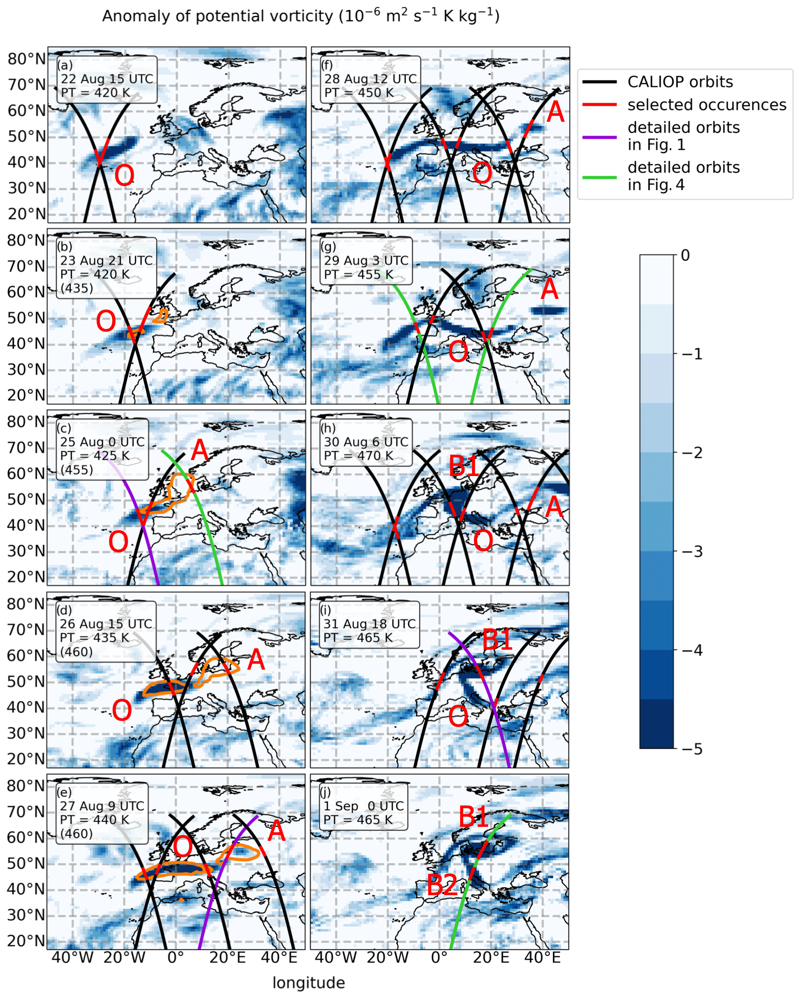
Figure 3Sequence of PV charts showing the splitting of vortex O into vortices A, B1 and B2. The map is plotted on the potential temperature surface corresponding to the core of vortex O or its continuation B2 in the ERA5 tracking. The orange lines are plotted at the isentropic level of vortex A, specified within parenthesis, and show the contour of −2 PVU (1 PVU = 10−6 ) for vortex A. The black, green and purple lines show the intersecting orbits of CALIPSO, and the red segments show the parts of the orbits occupied by the bubble (only the bubble core extent is displayed here). The maps are plotted at the hour that best matches the selected CALIOP occurrences. The purple orbits are those corresponding to the sections shown in Fig. 1; the green orbits are those corresponding to the sections shown in Fig. 4. Daytime and night-time orbits are used: the daytime orbits run from south-east to north-west, whereas the night-time orbits run from north-east to south-west. Starting from 1 September, the remainder of vortex O is relabelled as B2.
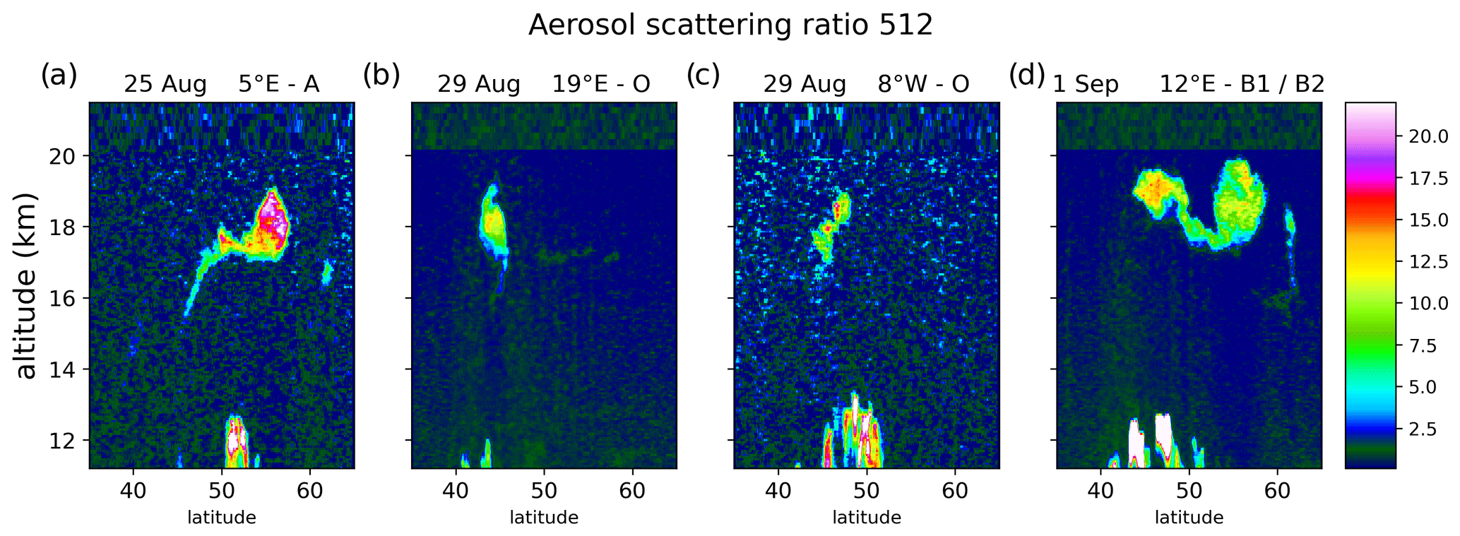
Figure 4Selection of four CALIOP scattering ratio sections of the smoke bubbles along the orbits shown in green in Fig. 3: (a) daytime section of bubble A on 25 August, (b) east night-time and (c) west daytime sections of elongated bubble O on 29 August, and (d) night-time double section of bubbles B1 (at ∼ 55∘ N) and B2 (at ∼ 45∘ N) on 1 September.
3.3 Horizontal and vertical splitting of vortex O into its offspring
Figure 3 displays the series of events that led, over the period from 22 August to 1 September, to the splitting of vortex O into its three offspring, which were subsequently followed over 1.5 months. We display the CALIPSO orbits that intersect the vortex cores as well as those that intersect their tails. The presence of a smoke bubble or patch detected by CALIOP along an orbit is shown as a red segment. For all orbits, we see that there are bubbles or patches that match each of the intersections with the tracked low-PV regions. The sequence begins on 22 August (Fig. 3a) with the elongated structure of vortex O that emerged at 420 K on the eastern flank of the trough within which it crossed the Atlantic. The elongation was due to the intense vertical shear in the jet stream. The formation of vortex A is already shown by the “rolling up” pattern on the north-east end of vortex O. On 23 August (Fig. 3b), the pattern of vortex A is lost at the 420 K level but is now visible at the 435 K level. A total of 2 d later (Fig. 3c), vortex A was a developed structure reaching 60∘ N at the 455 K level, and it was overflown by CALIPSO (Fig. 4a). At the same time, vortex O maintained a core near 45∘ N (Fig. 1d). In the following days, 26 and 27 August (Fig. 3d and e respectively), vortex A fully separated from vortex O as it moved eastward and rose (Fig. 1e). On 28 and 29 August (Fig. 3f and g respectively), vortex A moved away while vortex O was re-elongated and started to split into a western (Fig. 4b) and an eastern part (Fig. 4c). The vertical structure of vortex A on 28 August in another reanalysis is briefly shown in Fig. 16 of Allen et al. (2020). On 30 and 31 August (Fig. 3h and i respectively), the western part separated while the eastern part folded itself and separated into two more parts that provided vortex B1 as the northern component (Fig. 1) and vortex B2 as the southern component (essentially a continuation of vortex O), which were both seen on the same CALIOP overpass on 1 September (Figs. 3j and 4d). The B1 and B2 vortices fully separated in the following days while rising and starting to move slowly eastward. The western component could also be followed until 4 September, accompanied by patches seen by CALIOP; however, it remained below 460 K and could not be linked to any structure seen from CALIOP after 15 September with any certainty.
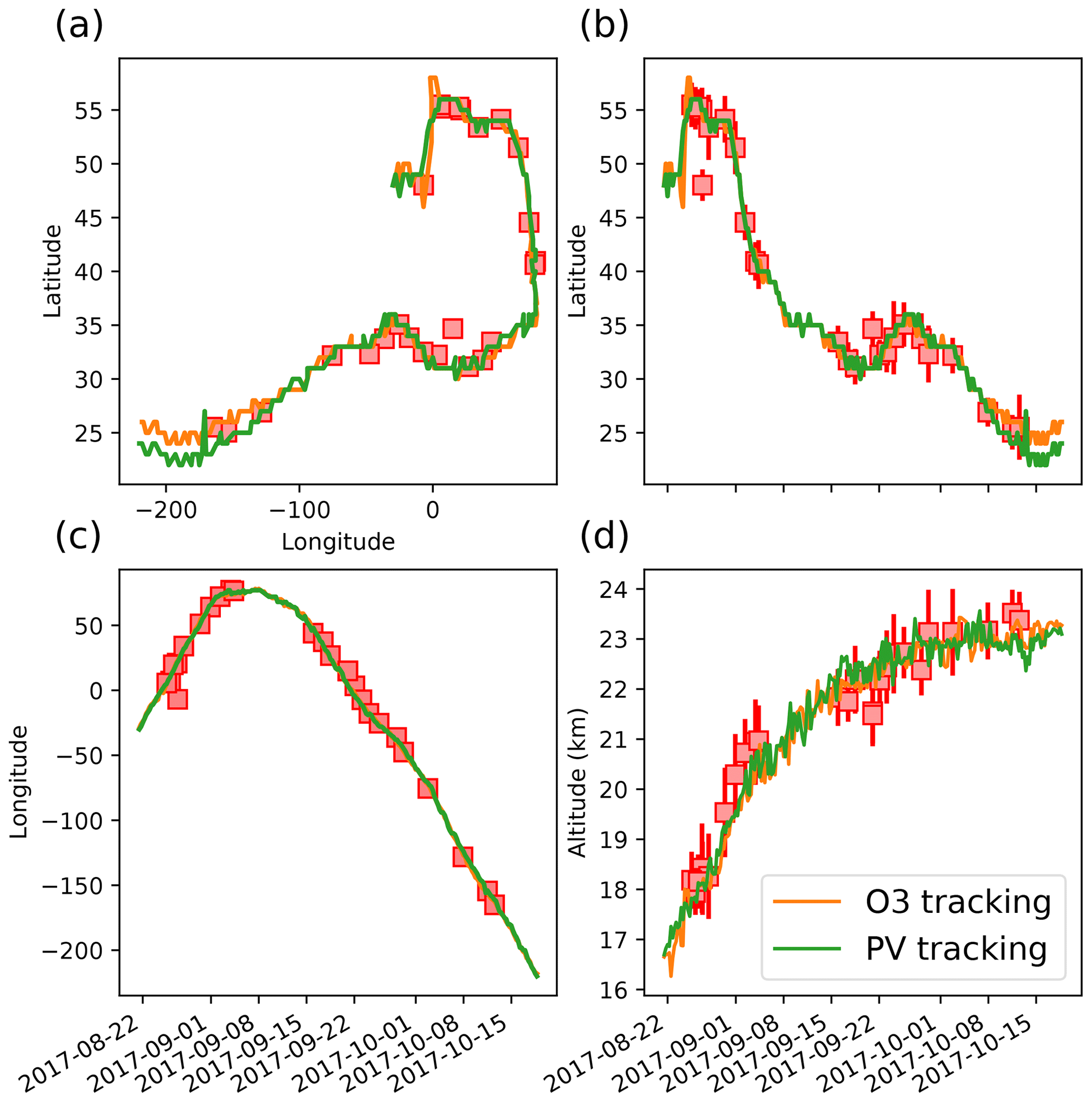
Figure 5The trajectory of vortex A tracked from the ERA5 fields of PV (orange) and ozone (green): (a) the trajectory in the longitude–latitude plane; (b–d) latitude, longitude and altitude as a function of time respectively. The green curves mostly mask the orange curves as they almost exactly coincide. The boxes show the location of the smoke bubble according to CALIOP during CALIPSO overpasses, and the bars indicate the range of the bubble in latitude and altitude.
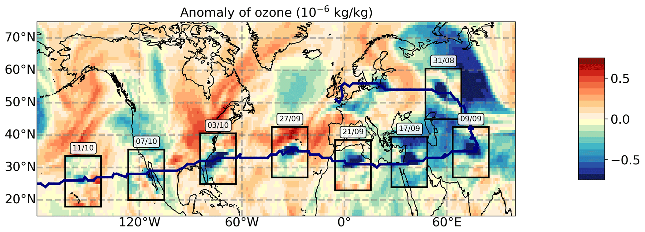
Figure 6Sequence of ozone anomalies along the trajectory of vortex A for selected dates from 31 August to 11 October. The background is the mean ozone anomaly over this period at 460 K. For each selected day, the box shows the ozone anomaly on that day at 00:00 UTC at the level of the vortex centroid according the ozone anomaly tracking, reported along the blue line.
3.4 Late evolution
During the observation period that followed the recovery of CALIOP after 15 September until mid-October, almost all observations of compact smoke bubbles at 20 km and above could be attributed to one of the vortices, A, B1 or B2. We discarded other observations of smoke patches that were under the shape of filaments. A number of these filaments belonged to tails left behind by the bubbles along their paths. As in Fig. 1, the location of the ERA5 vortex centre is shown using a cross in each panel of Fig. 2. The locations of the smoke bubble centres are shown as square marks in Fig. 5 which describes the trajectory of vortex A, and the bars indicate the latitudinal and altitudinal extent of the bubble. A perfect match with respect to the horizontal location is not expected, as there is no reason for the CALIPSO orbit to cross the vortex centre every time. Nevertheless, we see very good agreement between the ERA5 trajectory and the location of the 27 smoke bubbles seen by CALIOP that are attributed to vortex A, and the same holds for vortices B1 and B2 (Figs. S2 and S3 in the Supplement), both with 21 attributions. The evolution of vortices A, B1 and B2 is also available as animations in Sect. S3 of the Supplement. Vortex A was the first to separate from the mother vortex, vortex O, on 22 August, and it first moved eastward until it reached central Asia on 1 September at a latitude of 55∘ N and a longitude of 60∘ E. It then became trapped in the region of slow motion that extends between the two centres of the Asian monsoon anticyclone (AMA) and started to drift slowly southward while staying at about the same longitude and maintaining its ascent rate. A week later, it reached 35∘ N where it was caught in the easterly circulation and started to move westward, crossing Africa and continuing its path which could be tracked until the western Pacific. Figure 6 shows a composite image of successive images of the localized ozone hole from ERA5. It was easier to track the vortex using the ozone field than the PV. In particular, the PV signal almost vanished as it passed over Africa (see the vortex A animation in the Supplement), whereas the ozone signature was always very clear. We attribute the near disappearance of the PV signal to the strong infrared emissivity of the Sahara that limits the sensitivity of the Infrared Atmospheric Sounding Interferometer (IASI) sounders, which are important to sense the thermal signature of the vortex (Khaykin et al., 2020). The detection of ozone is less affected, as it also uses instruments such as the Global Ozone Monitoring Experiment-2 (GOME-2) (Khaykin et al., 2020) that operate in the ultraviolet range. The fact that the PV signature re-intensifies as soon as the vortex is over the Atlantic supports this hypothesis. During the last stages of the vortex, by mid-October, we also see a premature loss of the PV signal, whereas the ozone signal is still detectable and can be detected beyond the end of our tracking. This pattern is shared by the two other vortices, B1 and B2, and it differs from the 2020 case where an effect such as this is not observed for any of the vortices studied by Khaykin et al. (2020). Besides the increase in the IASI fleet, from two to three instruments, we do not see any drastic change in the observation system between the two events.
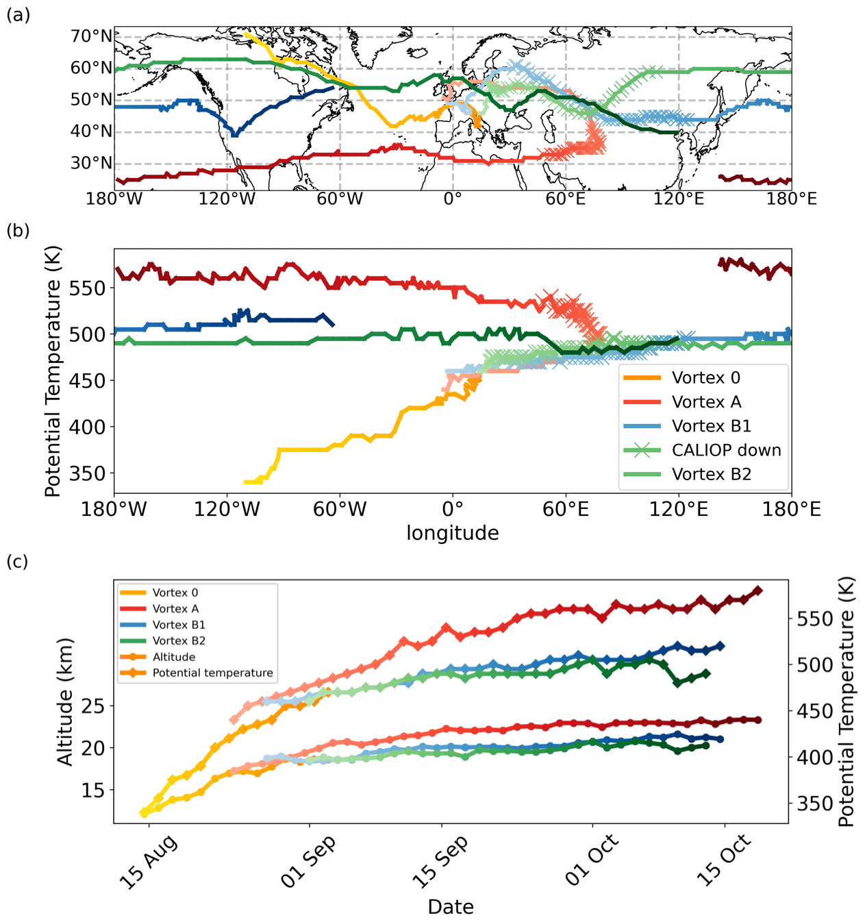
Figure 7Trajectories of the vortices based on the low-ozone anomaly from the ERA5 analysis at a 6 h sampling resolution. The colour gradient along each trajectory shows the time evolution of the vortices. We follow vortex O from 14 July 2017 until 31 August; it is then relabelled as vortex B2, and we follow its course until 11 October. Vortex A separates from vortex O on 22 August and is followed until 18 October. Vortex B1 separates from vortex O on 27 October and is followed until 14 October. Panel (c) shows the ascent in both altitude (left axis and lower set of curves) and potential temperature (right axis and upper set of curves). The crosses cover the part of each trajectory where CALIOP was not available.
While vortex A was completing its transition to the tropics, the two other vortices, B1 and B2, travelled eastward within the westerly flow on the northern side of the AMA, both reaching the Pacific on 18 September. Vortex B1 crossed the Pacific at mid-latitude and was lost near Hudson Bay after having crossed most of North America by 14 October. Vortex B2, which travelled at a higher latitude, completed a full round-the-world journey during the same period and was lost over central Asia by 11 October. Figure 7 summarizes the trajectories of vortices O, A, B1 and B2 from their formation to their loss. The total recorded paths of the four vortices are 13 000, 42 400, 28 500 and 33 400 km respectively. They rose up to 23 km for vortex A and to 21 km for vortices B1 and B2 (altitudes of the core).
3.5 Comparison with previous studies
Several previous studies have discussed the various stages of smoke cloud evolution described above, although none have made the link with a PV structure. Thus, a number of comments are in order here:
-
The ascent rate was the strongest during the initial stage of vortex O when it rose from its origin just above the tropopause. Previous studies based on CALIOP or limb-sounding instruments have reported an ascent rate using the upper envelop of the bubble. Yu et al. (2019) reported an ascent from 14 to 20 km from 15 to 24 August, and Khaykin et al. (2018) reported an ascent of 30 K d−1 in potential temperature (or 3 km d−1) between 16 and 18 August. We used the centroid of the PV and O3 anomalies to define the ascent and found (see Fig. S1 in the Supplement) that vortex O ascended from 12 to 17 km between 14 and 24 August, which is consistent with Yu et al. (2019), but we found no trace of a faster ascent. From 24 to 31 August, vortices O and A (see Fig. 5) climbed by 2 km, and vortex A maintained this rate until 8 September when it reached 21 km. It took 1 more month to reach the maximum altitude of 23 km, whereas B1 and B2 reached 21 km within the same time period. In the initial stage, Torres et al. (2020) claimed an ascent of 20 K d−1 on 14 August when the smoke bubble was detected in the stratosphere by CALIOP for the first time. However, the assumption of a tropopause crossing between 13 and 14 August is questionable, as the sections of CALIOP through the smoke cloud were on its periphery on 13 August, as shown by Fig. 1d of Torres et al. (2020) (even adding the missing night orbit). Therefore, it is equally plausible that the pyro-convective event directly injected smoke into the stratosphere without requiring large internal radiative heating.
-
Peterson et al. (2018) noticed the formation of vortex O from CALIPSO and Ozone Mapping and Profiler Suite (OMPS)/Suomi National Polar-orbiting Partnership (SUOMI NPP) overpasses on 14 August in northern Canada. Both Khaykin et al. (2018) and Peterson et al. (2018) reported that the first smoke patches had reached Europe by 19 August, and they were observed by a ground lidar station in central Europe on 22 August (Ansmann et al., 2018; Baars et al., 2019). These patches followed a northern route faster than that of vortex O and were seen as filamentary structures by CALIOP. Their forefront reached Asia by 24 August. By 29 August, a thick layer of smoke with an aerosol optical depth of 0.04 was seen from a lidar in south-eastern France at 19 km (Khaykin et al., 2018), corresponding to the passage of vortex O in the vicinity. According to our tracking, the lidar saw the tail connecting vortex O to vortex B1 during the course of separation (see Sect. 3.3). Bourassa et al. (2019) noticed the southward motion of vortex A over Central Asia but interpreted it as a split of the plume over this region on 1 September; however, the separation actually occurred 1 week before. It is tempting to see a trace of vortex A in the OMPS signal at 30∘ N above 20 km during September in Fig. 1 of Bourassa et al. (2019) and in the Stratospheric Aerosol and Gas Experiment III (SAGE III) low-latitude signal above 20 km during October in Fig. 1d of Kloss et al. (2019). Bourassa et al. (2019) were able to track smoke patches until January 2018, and the global signature at altitudes up to 24 km persisted until summer 2018 (Kloss et al., 2019).
-
Using several satellite instruments and transport calculations, Kloss et al. (2019) found the transport of smoke patches to the tropics taking place on the eastern southward branch of the AMA, but they excluded transport across the AMA which is what we observe for vortex A. These authors focused their work on the events of the last week of August and on levels below 20 km. The transition of vortex A occurred in early September and it was already above 20 km. The smoke layer that Kloss et al. (2019) subsequently followed in the tropics includes the effect of vortex A.
-
Baars et al. (2019) showed interesting evidence of aerosol patches over Europe and the Mediterranean area reaching 23 km by mid-September 2017 and again in mid-December 2017. Although unstated, they do not expect the second patches to be the remnant of the first. They instead provide an explanation based on a circuit identified by Kloss et al. (2019), where smoke patches were injected into the tropics in early September. The smoke then rose slowly to higher levels in the tropics and came back to the mid-latitudes carried by the Brewer–Dobson meridional circulation. There is, however, a hole in the reasoning of Baars et al. (2019): the tropical rise is reported to reach 21 km by March 2018, whereas the aerosols supposedly blown away by the Brewer–Dobson are found at 23 km over Europe in December 2017. It is now clear that the missing piece of the puzzle is provided by vortex A which reached 23 km by late September (with a top at 24–25 km) and left a tail along its path.
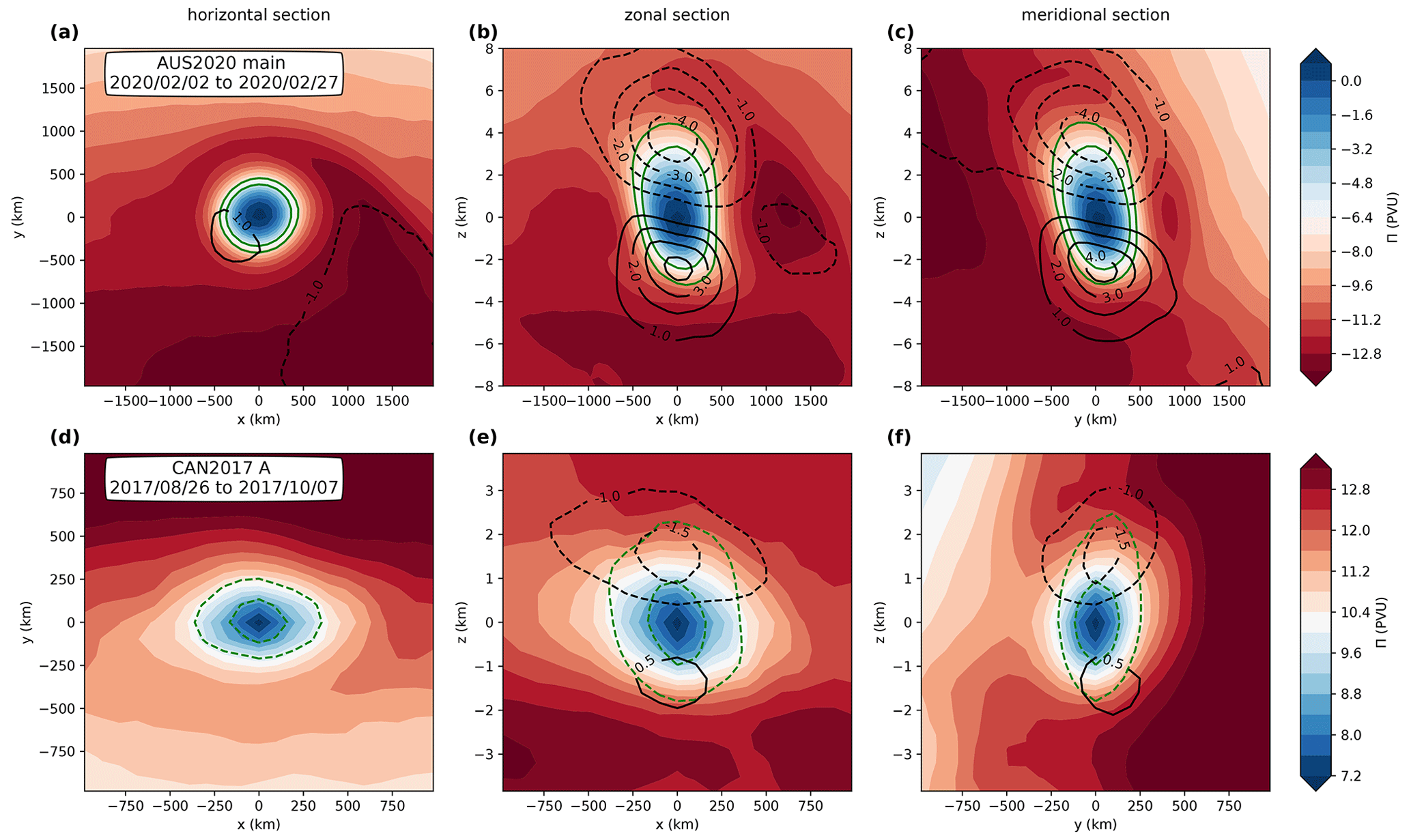
Figure 8Time-averaged composite sections of Lait PV Π, in PVU (1 PVU = 10−6 ), following two selected smoke-charged vortices, the main Koobor vortex from the 2020 Australian wildfires described in Khaykin et al. (2020) (a–c) and vortex A introduced in this paper (d–f). Panels (a) and (d), (b) and (e), and (c) and (f) show the respective horizontal, zonal and meridional sections through the centroid of the vortex. The green lines are contours of anticyclonic vertical vorticity (corresponding to 3 × 10⁻⁵ and 5 × 10⁻⁵ s−1 for panels a–c, and −1.5 × 10⁻⁵ and −2.5 × 10⁻⁵ s−1 for panels d–f). The black contours are the temperature anomaly with respect to the zonal mean. Note that the horizontal and vertical ranges displayed are reduced by a factor of 2 for vortex A.
4.1 Composite analysis of the vortices in ERA5
Here, we investigate the structure of the vortices by the mean of a composite analysis. The dynamical fields surrounding the vortex centroids were re-gridded regularly in Cartesian geometry in the horizontal and in log-pressure altitude (Andrews et al., 1987) in the vertical, within a moving frame that follows the centroids' ascent and horizontal displacement. As in Khaykin et al. (2020), the composite model fields were then averaged in time to generate a composite analysis that filters out noise and variability unrelated to the vortices. This procedure also removes short-term vacillations (see Khaykin et al., 2020; Allen et al., 2020) which are a common property of vortices in shear flow (e.g. Tsang and Dritschel, 2015), thereby enabling us to emphasize the mean structure of the vortex. Figure 8 depicts the composite of Lait PV Π (defined in Eq. 2) and the temperature anomaly following vortex A (Fig. 8d–f) and the main Koobor vortex (Fig. 8a–c) generated by the 2020 Australian fires and tracked by Khaykin et al. (2020). In the natural coordinates, without expanding the vertical direction, both vortices appear as isolated pancakes of anomalous anticyclonic Lait PV (i.e. negative in the Northern Hemisphere and positive in the Southern Hemisphere). The analysed temperature anomaly consists of a vertical dipole surrounding the PV monopole with a negative temperature anomaly above and a positive temperature below it, whose centres are located on the upper and lower edges of the Lait PV distribution. As noted by Khaykin et al. (2020), this relationship between temperature stratification and vorticity is qualitatively consistent with the thermal wind balance and is characteristic of anticyclonic vortices in the quasi-geostrophic (QG) equations (Dritschel et al., 2004) as well as of balanced anticyclones in the full primitive equations (e.g. Hoskins et al., 1985). In the case of the smoke-charged vortices investigated here, it turns out that their intensity is slightly beyond that of the typical geostrophic flow. The typical Rossby number of the structure can be expressed as follows:
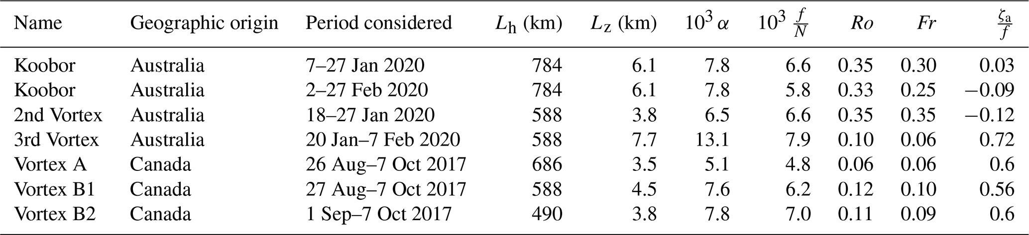
where U is the maximum horizontal wind speed, Lh is the horizontal length scale (defined as the diameter of the ring of the local wind speed maximum at the altitude of the centroid and estimated in the west–east direction) and is the average relative vorticity. Ro is about 0.06 in the 2017 case and 0.35 for 2020. While the Rossby number is beyond the typical QG regime (Ro<0.1) in 2020, the aspect ratio α, defined as
(where Lz is the vertical extent of the contour of vorticity at maximum wind speed at the horizontal location of the vortex centroid), obeys the stratified QG scaling in both cases, despite the 2017 vortex A being about 2.3 times smaller in volume than its gigantic 2020 counterpart.
Table 1The horizontal diameter (Lh), vertical depth (Lz), aspect ratio (α), QG aspect ratio imposed by the environment (), Rossby number, Froude number and maximum vorticity () of the six smoke-charged pancake vortices originating from the Canadian (2017) and Australian (2020) wildfires. The 2020 Koobor vortex was long-lasting and is decomposed into two periods here.
To further investigate the dynamical regime in which the identified vortices evolve (or their representation in the IFS), Table 1 presents their typical sizes; their amplitude characterized by the Rossby number Ro and the Froude number,
and the absolute vorticity amplitude at the vortex centroid normalized by f,
which measures the inertial (in)stability of the flow. It should be noted that despite the similarity, is not redundant with Ro defined in Eq. (3) and characterizes the extremum rather than the structure average of the vorticity.
Keeping the limited vertical and horizontal resolution of the IFS in mind, it can be noticed that the Froude and Rossby numbers are always of the same order, leading to a Burger number Bu∼1, as typically encountered in geophysical flows. Furthermore, most vortices in Table 1 obey the QG aspect ratio, so that they are quasi-spherical (see Fig. 8) when the vertical coordinate is stretched by a factor . This observation is consistent with numerical studies of ellipsoidal vortices, which have demonstrated the higher stability of quasi-spherical vortices (Dritschel et al., 2005) and the tendency of aspherical vortices to relax towards sphericity in the stretched coordinate system (Tsang and Dritschel, 2015).
Contrary to its aspect ratio, the magnitude of the vortex perturbation is case-dependent and does not necessarily fit in the classical QG scaling, thereby contrasting with the synoptic-scale circulation. Indeed, typical vortex-averaged Rossby numbers range from 0.06 up to 0.35, a range similar to observed mesoscale and sub-mesoscale oceanic eddies (e.g. Le Vu et al., 2017). For the intense 2020 Koobor vortex, the maximum vorticity in the vortex core is on the verge of inertial instability or even slightly beyond its threshold for linear flows (Hoskins, 1974), as can be seen from the positive Π values in Fig. 8 (see also the small negative values of in Table 1). This property was maintained over 1.5 months from the formation of the Koobor vortex to its first breaking (see Fig. S4 in the Supplement). Although it is not clear how realistic the ECMWF vortices are, their amplitude is likely underestimated as they are forced by data assimilation and the stand-alone model does not simulate them. Therefore, we cannot generally conclude on the amplitude of the perturbations, in particular that of the smaller Northern Hemisphere vortices. Nevertheless, the 2020 cases demonstrate that the vorticity anomaly may reach the threshold for inertial instability at which it likely saturates.
Related to their different magnitudes, the vortices also have distinct impacts on their immediate surroundings, as can be identified in Fig. 8. While the 2020 Koobor vortex was strong enough to generate a significant cyclonic PV anomaly eastward of the vortex centroid which rolls up around it on its northern edge, no such signature can be distinguished around vortex A. In a zonal plane, the 2020 negative PV patch has diameter comparable to the Koobor vortex but a reduced magnitude. The existence of this negative anomaly can be attributed to the equatorward advection of cyclonic PV on the eastern flank of Koobor and is likely responsible for the equatorward beta-drift (Lam and Dritschel, 2001) undergone by Koobor during its ascent.
Finally, for completeness, two further remarks should be made. First, the reader should note that the vertical temperature dipole is slightly asymmetric with a larger magnitude of the negative temperature anomaly. Second, Fig. 8c shows that the vertical axis of Koobor exhibits on average a small tilt with altitude, being slanted along the south–north direction, which is perpendicular to the prevailing background shear. This property is a common characteristic of vortices undergoing shear (Tsang and Dritschel, 2015) and is related to the temporal vacillations of Koobor described by Allen et al. (2020) and also seen in Fig. 6 of Khaykin et al. (2020).
4.2 Diagnosing diabatic tendencies
By comparing the 2020 Koobor vortex in the ECMWF analyses and model forecasts, Khaykin et al. (2020) showed systematic shortcomings of the free-running model with respect to the analysis, namely
-
a failure to reproduce the observed ascent of the structure at about 6 K d−1 in potential temperature – on the contrary, the modelled anticyclones tend to remain at constant θ;
-
a decay of the vorticity anomaly within 1 week, whereas the observed vortex survives for more than 3 months.
This suggests that data assimilation of observed temperature and ozone profiles is a necessary ingredient to both the ascent and the maintenance of the vortex in the model, whereas some physical or spurious processes act to dissipate the structure. In the atmosphere, it is assumed that the forcing is exerted by radiative heating through solar absorption by black carbon aerosols within the smoke (Yu et al., 2019). Thus, increments are expected to be a substitute in the analysis system for the diabatic tendency maintaining the vortices, as wildfire smoke is missing from the model.
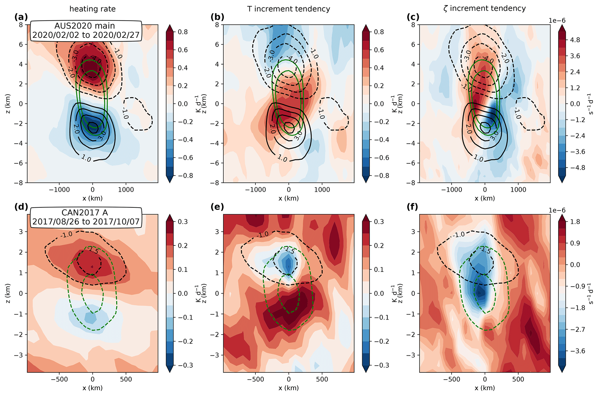
Figure 9Time-averaged composite sections of the ERA5 total heating rate (a, c), increment-induced temperature (b, e) and vorticity tendency (c, f) following two selected smoke-charged vortices, the major vortex from the 2020 Australian wildfires described in Khaykin et al. (2020) (a–c) and vortex A (d–f). The green lines are contours of anticyclonic vertical vorticity (corresponding to 3 × 10⁻⁵ and 5 × 10⁻⁵ s−1 for panels a–c, and −1.5 × 10⁻⁵ and −2.5 × 10⁻⁵ s−1 for panels d–f). The black contours are the temperature anomaly with respect to the zonal mean. Note that the displayed horizontal range is reduced by a factor of 2 for vortex A.
4.2.1 Temperature and vorticity tendencies
Figure 9a and d depict the average composite of the ERA5 total heating due to physics calculated over the forecast. This field is dominated by the longwave radiative heating component as the shortwave absorption by the smoke is missing from the IFS. The dominant feature shown by Fig. 9 is a damping of the temperature anomaly T′ with respect to the radiative equilibrium temperature which can be cast into a Newtonian relaxation as follows:
where τrad is the radiative damping rate. Figure 9 suggests τrad ≃ 6–7 d. This is consistent with the lifetime of the structure in the ECMWF forecast which is about 1 week (Khaykin et al., 2020), suggesting that radiative dissipation plays a major role in the decay of the vortex in the model but also in the real atmosphere.
However, as the model itself cannot sustain the vortices, it comes down to data assimilation to maintain the structure. Khaykin et al. (2020) demonstrated that the IFS extracts information from the thermal signature and the ozone anomaly detected by satellite instruments. The temperature increments are shown in Fig. 9b and e. In contrast to the heating rates, which are instantaneous forcing of the temperature by physical processes, the temperature increments result from the balanced dynamical response of the temperature field to the forcing induced by the discrepancy of measured radiances with respect to their estimated values in the assimilation procedure. Hence, the temperature pattern does not match the observed aerosol bubble co-located with the vortex which would be expected for the shortwave aerosol absorption; rather, it exhibits a multipolar structure, essentially oriented vertically. In the 2017 case with a limited vertical ascent rate, the T increment vertical dipole mainly cancels the radiative damping. In 2020, it is rather a tripole that enables the maintenance and the ascent of the dipolar temperature anomaly structure.
Due to this dynamical adjustment, temperature is not the only field incremented via data assimilation. Figure 9c and f show the increments of relative vorticity ζ. They contribute again to the maintenance (2017 case) and the ascent and maintenance (2020 case) of the vortices. Moreover, similarly to the composite vortex, the composite vorticity and temperature increment tendencies exhibit the structure of a balanced vortex: the 2017 anticyclonic ζ tendency monopole is sandwiched between the two extrema of the temperature increment dipole, whereas the tripole of the T increment alternates with the two layers of vorticity anomalies in 2020. Overall, the T and ζ patterns of the 2020 assimilation increment are qualitatively consistent with the expected effect of localized heating in a rotating atmosphere (as sketched in Fig. 10 of Hoskins et al., 2003).
Together with the apparently balanced vortex structure of the increments, the similarity to the theoretical response in Hoskins et al. (2003) suggests that potential vorticity (or Lait PV) is the appropriate field to consider for a more straightforward interpretation of the increments in terms of missing diabatic processes. This is the focus of the next subsection.

4.2.2 Lait PV and ozone tendencies due to assimilation increments
Composite time-averaged increments of Lait PV Π are presented in Fig. 10. As stressed above, Π increments result from a combination of both temperature and vorticity and appear due to the implicit incorporation of temperature observations into an approximately dynamically balanced response by the 4D-Var scheme used in ERA5.
Contrary to the mean vortex structure in Fig. 8, we notice a stark contrast between the Northern Hemisphere and Southern Hemisphere vortices. In the 2017 case, the Π increment shows a dominant monopole structure whose extremum is slightly shifted upward (by about 500 m) with respect to the Π extremum (Fig. 8). Thus, the effect of the increment is mainly to reinforce the existing Π anomaly and, secondarily, to drive its ascent. In contrast, the 2020 case essentially shows a vertical dipole structure which forces an ascent of the Π centre. Furthermore, the dipole is tilted along a north-west to south-east axis. A qualitative analysis (Appendix B) shows that the observed westward tilt of the increment dipole emerges as a consequence of the negative zonal wind shear encountered by the 2020 Koobor vortex along its ascent. More precisely, it is the combination of this shear and the distribution of the increment tendency over the 12 h analysis time window which is responsible for the tilt. This feature may also be seen during other periods of the Koobor's lifetime during which the structure was drifting eastward, such as in the middle of January 2020 (see Fig. B1), emphasizing that the inclination of the increment dipole is due to the background wind shear rather than the local wind at the altitude of the vortex.
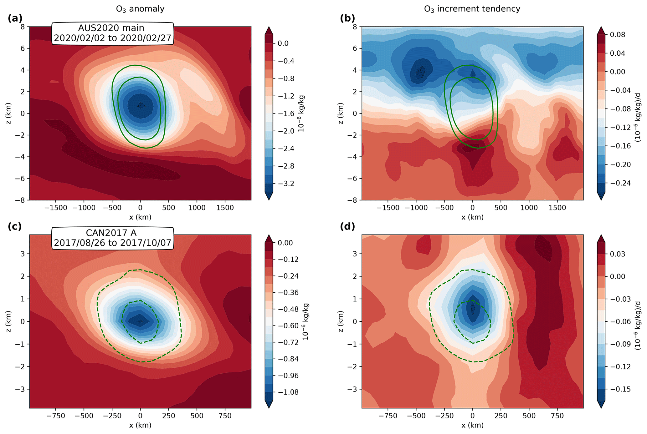
Figure 11Same as Fig. 9 but for ozone anomalies from the zonal mean (a, c) and ozone increments (b, d).
The different patterns of Lait PV Π (Fig. 8) and its increment (Fig. 10) around the vortex are mimicked in the ozone field, as shown in Fig. 11. As described above, the ascending anticyclonic vorticity anomalies are accompanied by negative ozone anomalies (Fig. 11a, c). Compared with Figs. 8 and 10, Fig. 11 shows that the patterns of the ozone anomaly bubble and its increment are very similar to those of Π. We note that the magnitude of the increments may vary depending on the period chosen for the composite – for instance, due to the different ascent speed of the vortex in the log-pressure altitude coordinate (250 m d−1 in January vs. 150 m d−1 in February for Koobor). However, the monopole and tilted dipole structures shown in Figs. 10 and 11 are representative of the typical situation found. Overall, model increments tend to (i) counter the dissipation and (ii) drive a cross-isentropic vertical motion of PV and ozone anomalies.
At this point, it is tempting to interpret the low-ozone, low-absolute-PV anticyclones as resulting from the vertical advection of smoke-charged tropospheric air bubbles conserving both their low absolute PV and their tropospheric tracer content during their ascent in the stratosphere. In the case of the 2020 Koobor vortex, this perception is broadly consistent with the behaviour of absolute PV and the PV anomaly at the centre of the vortex, which remains constant or exhibits a steady increase related to the large vertical gradient of PV within the stratosphere respectively (Fig. S4 in the Supplement). It is also consistent with our analysis of the developing stage of the mother vortex O in Sect. 3.2. We note, however, that the analogy between inert tracer and PV transport arises from their Lagrangian conservation in the adiabatic inviscid case and breaks in the presence of diabatic processes (Haynes and McIntyre, 1987). Hence, the maintenance of this relationship calls for dedicated theoretical and numerical investigations.
The generation of smoke-charged vortices rising in the Southern Hemisphere stratosphere was discovered following the Australian wildfires at the end of 2019 (Khaykin et al., 2020). Here, we find that similar events took place in 2017 in the Northern Hemisphere stratosphere after the British Columbian wildfires that culminated in early August 2017 when a large plume of smoke and low-potential-vorticity air was injected into the lower stratosphere on 12 August 2017. We show that a vortical structure developed in the plume soon after injection and started to rise in the stratosphere. During the following days, this smoke vortex became an isolated bubble and was transported eastward across the Atlantic while becoming elongated due to wind shear and reaching 19 km in altitude at its top. Subsequently, the structure was split into three separate vortices over western Europe that could be followed until the middle of October 2017. Two of the vortices kept moving eastward in the middle latitudes and performed a round-the-world journey, rising up to a potential temperature of 530 K (21 km). The third one transited to the subtropics across the Asian monsoon anticyclone and moved eastward until Asia. It also rose higher, reaching 570 K (23 km).
Our study again demonstrates the ability of the advanced assimilation system used at the ECMWF, which is the basis of ERA5, to exploit the signature left by smoke vortices in the temperature and ozone fields and reconstruct the balanced vortical structure. The balance is produced during the iterations of the assimilation; therefore, the assimilation increment reflects this balance by providing an increment on the wind as well as on the temperature. The increment is consistent with the expected effect of a localized heating due to the radiative absorption of the smoke. It fights the longwave radiative dissipation and moves the vortices upward. It is quite likely, however, that the detection of vortices by the assimilation system is limited by the sensitivity of the satellite instruments to the disturbances in the temperature and ozone fields. There are also detection limits for CALIOP and limited chances to overpass small-scale structures if they are sparse enough. Therefore, it is possible that a number of small-scale vortices escaped the direct methods used in this study. It is also possible that dynamical constraints, like the ambient shear, limit the existence of such vortices. Hence, based on our study, it is difficult to make conclusions regarding the generality of such structures and what their global impact may be. However, it is quite clear that they provide an effective way for smoke plumes to remain compact and concentrated, inducing a rise of the order of 10 km or more in the stratosphere that, in turn, increases the lifetime and the radiative impact mentioned in previous studies (Ditas et al., 2018) from months to years knowing the character of the Brewer–Dobson circulation (e.g. Butchart, 2014).
Long-lived anticyclones dubbed as “frozen-in anticyclones” (FrIAC) by Manney et al. (2006) have already been reported in the Arctic stratosphere. They share a long lifespan with the smoke anticyclones, but they differ in many other respects. The FrIAC are deep barotropic structures extending from 550 to 1300 K and are observed in the polar region after the breaking of the winter polar vortex. They are generated by the isentropic intrusion of low-latitude air with low PV (Allen et al., 2011; Thiéblemont et al., 2011). Instead, the smoke vortices exhibit a strong baroclinic structure with a vertical temperature dipole and are propelled through the layers of the stratosphere by their internal heating bringing tropospheric air to the middle stratosphere at latitudes where the Brewer–Dobson circulation does the opposite (Butchart, 2014).
As volcanic plumes in the stratospheric are usually made of secondary sulfuric acid aerosols that are considerably less absorbing than black carbon, rising compact plumes are not expected to be seen in the stratosphere after extratropical volcanic eruptions. Such a case, however, was reported after the 2019 eruption of Raikoke (Chouza et al., 2020; Muser et al., 2020). This event which displays a slow rise and is not associated with a vortex in ERA5 might fall below the detection limit, but it poses a question regarding the possible role of heating by volcanic aerosols.
The conditions to maintain the stability of the smoke vortices and those leading to their final dilution are also not yet understood, and this work is only opening a path to be explored.
Figure A1 shows two screenshots as examples of the interactive tracking of the smoke bubbles in CALIOP sections of the scattering ratio. The first case (Fig. A1a) is taken from bubble O on 19 August when it was elongated within the Atlantic trough. The second case (Fig. A1b) is taken from bubble A on 24 September while it was moving westward over the Atlantic. The interactive method used to perform the tracking is displayed in an animation in Sect. S1 of the Supplement.

Figure A1CALIOP sections with the superimposed box showing how the interactive tracking is performed: (a) daytime orbit over bubble O on 19 August, and (b) night-time orbit over bubble A on 24 September.
The average composite of the Lait PV increment for the 2020 anticyclone (Fig. 10) exhibits a tilted dipole structure whose inclination by far exceeds the slight dip observed for the vortex axis and shown by the green vorticity contours in Fig. 10b. This tilt causes the dipole to appear not only in vertical panes but also in the horizontal one (Fig. 10a). The existence of the tilt is not related to the direction of the drift of the vortex: in January, when Koobor is drifting eastward due to the prevailing westerlies, we observe the same general orientation of the increment dipole, as shown in Fig. B1.
From a purely kinematic point of view, the dipolar structure of the increment shows that the forecast model systematically underestimates both upward and westward motions (as well as northward in Fig. B1). While it is unlikely that the ECMWF forecast model underestimates zonal wind magnitude over such a long period, this missing westward displacement filled by the increments may be attributed to missing vertical ascent in an easterly sheared background wind.
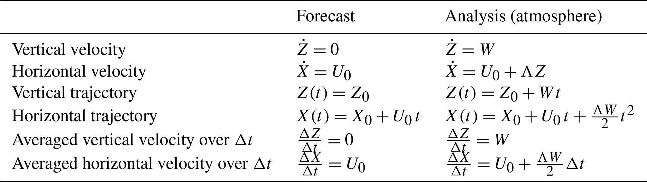
This can be grasped by comparing trajectories advected by a sheared flow (wind profile , where Λ is the shear) with or without an ascent. The two situations are contrasted for a simplified case in Table B1. Over the finite analysis time window (Δt), the vertical ascent rate (W) causes the parcel (here, the vortex) to be advected in a region of different mean wind and to drift away from its non-ascending cousin. Hence, the additional motion brought by the ascent has both vertical and horizontal components, which can be expressed as follows:
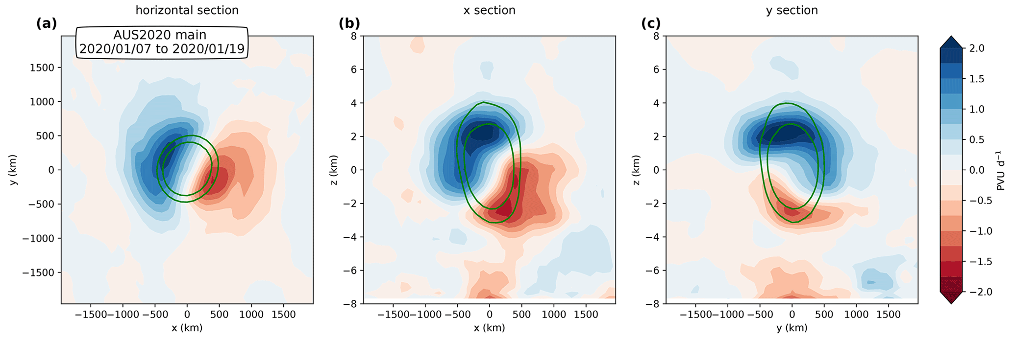
Figure B1Same as Fig. 10 but for the Koobor Lait PV increments during the 7–19 January 2020 time period. Note the different colour bar compared with Fig. 10. The different magnitude of the increments is due to the contrasting ascent speed of the vortex in the log-pressure altitude coordinate (250 m d−1 in January vs. 150 m d−1 in February).
The tendency of Π associated with a translation at speed is
If we consider the isolated bubble of maximum potential vorticity anomaly Pmax and length scales Lx and Lz=αLx, the magnitude of the tendency required to translate it along x and z are then
and their ratio γ is
In the case of the 2020 vortex, and the background shear Λ estimated in a 8 km layer around the vortex varies from ≃ −3 × 10⁻³ s−1 between 7 and 19 January to ≃ −2 × 10⁻³ s−1 between 2 and 27 February. With those values and the assimilation window Δt = 0.5 d, is of the order of 0.3 to 0.5, which is quantitatively consistent with Figs. 10b and B1. When the shear is properly taken into account, the westward drift induced by the increments can thus be reconciled with the idea that the ascent is the main process lacking from the model. Note that this reasoning also applies to ozone.
Table B1Analytical trajectory of a bubble in an idealized sheared wind profile: with (forecast) or without (analysis) vertical ascent, and the resulting average speed.
The programs used in this work are available on GitHub at https://github.com/aurelien-podglajen/Astus (aurelien-podglajen, 2021), https://github.com/hugolestrelin/CAN2017_pyrocb_stratovortex (hugolestrelin, 2021) and https://github.com/bernard-legras/STC-CAN (bernard-legras, 2021a) and depend on https://github.com/bernard-legras/STC/tree/master/pylib (bernard-legras, 2021b).
CALIOP data were provided by the ICARE/AERIS data centre. ERA5 data were provided by the Copernicus Climate Change Service.
The supplement related to this article is available online at: https://doi.org/10.5194/acp-21-7113-2021-supplement.
HL, BL, Ap and MS performed the analysis. HL, BL and AP wrote the original version of the paper. All authors contributed the final article.
The authors declare that they have no conflict of interest.
This work was supported by the TTL-Xing ANR-17-CE01-0015 project of the Agence Nationale de la Recherche.
This paper was edited by Peter Haynes and reviewed by three anonymous referees.
Allen, D. R., Douglass, A. R., Manney, G. L., Strahan, S. E., Krosschell, J. C., Trueblood, J. V., Nielsen, J. E., Pawson, S., and Zhu, Z.: Modeling the Frozen-In Anticyclone in the 2005 Arctic Summer Stratosphere, Atmos. Chem. Phys., 11, 4557–4576, https://doi.org/10.5194/acp-11-4557-2011, 2011. a
Allen, D. R., Fromm, M. D., Kablick III, G. P., and Nedoluha, G. E.: Smoke with Induced Rotation and Lofting (SWIRL) in the Stratosphere, J. Atmos. Sci., 77, 4297–4316, https://doi.org/10.1175/JAS-D-20-0131.1, 2020. a, b, c, d
Andrews, D., Holton, J., and Leovy, C.: Middle Atmosphere Dynamics, Academic Press, London, 1987. a, b
Ansmann, A., Baars, H., Chudnovsky, A., Mattis, I., Veselovskii, I., Haarig, M., Seifert, P., Engelmann, R., and Wandinger, U.: Extreme levels of Canadian wildfire smoke in the stratosphere over central Europe on 21–22 August 2017, Atmos. Chem. Phys., 18, 11831–11845, https://doi.org/10.5194/acp-18-11831-2018, 2018. a, b
aurelien-podglajen: Astus, GitHub, available at: https://github.com/aurelien-podglajen/Astus, last access: 10 May 2021. a
Baars, H., Ansmann, A., Ohneiser, K., Haarig, M., Engelmann, R., Althausen, D., Hanssen, I., Gausa, M., Pietruczuk, A., Szkop, A., Stachlewska, I. S., Wang, D., Reichardt, J., Skupin, A., Mattis, I., Trickl, T., Vogelmann, H., Navas-Guzmán, F., Haefele, A., Acheson, K., Ruth, A. A., Tatarov, B., Müller, D., Hu, Q., Podvin, T., Goloub, P., Veselovskii, I., Pietras, C., Haeffelin, M., Fréville, P., Sicard, M., Comerón, A., Fernández García, A. J., Molero Menéndez, F., Córdoba-Jabonero, C., Guerrero-Rascado, J. L., Alados-Arboledas, L., Bortoli, D., Costa, M. J., Dionisi, D., Liberti, G. L., Wang, X., Sannino, A., Papagiannopoulos, N., Boselli, A., Mona, L., D'Amico, G., Romano, S., Perrone, M. R., Belegante, L., Nicolae, D., Grigorov, I., Gialitaki, A., Amiridis, V., Soupiona, O., Papayannis, A., Mamouri, R.-E., Nisantzi, A., Heese, B., Hofer, J., Schechner, Y. Y., Wandinger, U., and Pappalardo, G.: The unprecedented 2017–2018 stratospheric smoke event: decay phase and aerosol properties observed with the EARLINET, Atmos. Chem. Phys., 19, 15183–15198, https://doi.org/10.5194/acp-19-15183-2019, 2019. a, b, c, d
bernard-legras: STC-CAN, GitHub, available at: https://github.com/bernard-legras/STC-CAN, last access: 10 May 2021. a
bernard-legras: STC, GitHub, available at: https://github.com/bernard-legras/STC/tree/master/pylib, last access: 10 May 2021. a
Bourassa, A. E., Rieger, L. A., Zawada, D. J., Khaykin, S., Thomason, L. W., and Degenstein, D. A.: Satellite Limb Observations of Unprecedented Forest Fire Aerosol in the Stratosphere, J. Geophys. Res.-Atmos., 124, 9510–9519, https://doi.org/10.1029/2019JD030607, 2019. a, b, c, d
Butchart, N.: The Brewer–Dobson Circulation, Rev. Geophys., 52, 157–184, https://doi.org/10.1002/2013RG000448, 2014. a, b
Chouza, F., Leblanc, T., Barnes, J., Brewer, M., Wang, P., and Koon, D.: Long-term (1999–2019) variability of stratospheric aerosol over Mauna Loa, Hawaii, as seen by two co-located lidars and satellite measurements, Atmos. Chem. Phys., 20, 6821–6839, https://doi.org/10.5194/acp-20-6821-2020, 2020. a
de Laat, A. T. J., Stein Zweers, D. C., Boers, R., and Tuinder, O. N. E.: A Solar Escalator: Observational Evidence of the Self-Lifting of Smoke and Aerosols by Absorption of Solar Radiation in the February 2009 Australian Black Saturday Plume: OBSERVATIONS OF SELF-LIFTING AEROSOLS, J. Geophys. Res.-Atmos., 117, D04204, https://doi.org/10.1029/2011JD017016, 2012. a
Ditas, J., Ma, N., Zhang, Y., Assmann, D., Neumaier, M., Riede, H., Karu, E., Williams, J., Scharffe, D., Wang, Q., Saturno, J., Schwarz, J. P., Katich, J. M., McMeeking, G. R., Zahn, A., Hermann, M., Brenninkmeijer, C. A. M., Andreae, M. O., Pöschl, U., Su, H., and Cheng, Y.: Strong Impact of Wildfires on the Abundance and Aging of Black Carbon in the Lowermost Stratosphere, P. Natl. Acad. Sci. USA, 115, E11595–E11603, https://doi.org/10.1073/pnas.1806868115, 2018. a, b
Dritschel, D. G., Reinaud, J. N., and McKiver, W. J.: The quasi-geostrophic ellipsoidal vortex model, J. Fluid Mech., 505, 201–223, https://doi.org/10.1017/S0022112004008377, 2004. a
Dritschel, D. G., Scott, R. K., and Reinaud, J. N.: The Stability of Quasi-Geostrophic Ellipsoidal Vortices, J. Fluid Mech., 536, 401–421, https://doi.org/10.1017/S0022112005004921, 2005. a
Ertel, H.: Ein neuer hydrodynamischer Erhaltungssatz, Die Naturwissenschaften, 30, 543–544, https://doi.org/10.1007/BF01475602, 1942. a
Fromm, M., Lindsey, D. T., Servranckx, R., Yue, G., Trickl, T., Sica, R., Doucet, P., and Godin-Beekmann, S.: The Untold Story of Pyrocumulonimbus, B. Am. Meteorol. Soc., 91, 1193–1210, https://doi.org/10.1175/2010BAMS3004.1, 2010. a, b
Hanes, C. C., Wang, X., Jain, P., Parisien, M.-A., Little, J. M., and Flannigan, M. D.: Fire-regime changes in Canada over the last half century, Can. J. Forest Res., 49, 256–269, https://doi.org/10.1139/cjfr-2018-0293, 2019. a, b
Haynes, P. H. and McIntyre, M. E.: On the Evolution of Vorticity and Potential Vorticity in the Presence of Diabatic Heating and Frictional or Other Forces, J. Atmos. Sci., 44, 828–841, https://doi.org/10.1175/1520-0469(1987)044<0828:OTEOVA>2.0.CO;2, 1987. a
Hersbach, H., Bell, B., Berrisford, P., Hirahara, S., Horányi, A., Muñoz-Sabater, J., Nicolas, J., Peubey, C., Radu, R., Schepers, D., Simmons, A., Soci, C., Abdalla, S., Abellan, X., Balsamo, G., Bechtold, P., Biavati, G., Bidlot, J., Bonavita, M., Chiara, G. D., Dahlgren, P., Dee, D., Diamantakis, M., Dragani, R., Flemming, J., Forbes, R., Fuentes, M., Geer, A., Haimberger, L., Healy, S., Hogan, R. J., Hólm, E., Janisková, M., Keeley, S., Laloyaux, P., Lopez, P., Lupu, C., Radnoti, G., de Rosnay, P., Rozum, I., Vamborg, F., Villaume, S., and Thépaut, J.-N.: The ERA5 global reanalysis, Q. J. Roy. Meteor. Soc., 146, 1999–2049, https://doi.org/10.1002/qj.3803, 2020. a
Hoffmann, L., Günther, G., Li, D., Stein, O., Wu, X., Griessbach, S., Heng, Y., Konopka, P., Müller, R., Vogel, B., and Wright, J. S.: From ERA-Interim to ERA5: the considerable impact of ECMWF's next-generation reanalysis on Lagrangian transport simulations, Atmos. Chem. Phys., 19, 3097–3124, https://doi.org/10.5194/acp-19-3097-2019, 2019. a
Hoskins, B., Pedder, M., and Jones, D. W.: The Omega Equation and Potential Vorticity, Q. J. Roy. Meteor. Soc., 129, 3277–3303, https://doi.org/10.1256/qj.02.135, 2003. a, b
Hoskins, B. J.: The Role of Potential Vorticity in Symmetric Stability and Instability, Q. J. Roy. Meteor. Soc., 100, 480–482, https://doi.org/10.1002/qj.49710042520, 1974. a
Hoskins, B. J., McIntyre, M. E., and Robertson, A. W.: On the Use and Significance of Isentropic Potential Vorticity Maps, Q. J. Roy. Meteor. Soc., 111, 877–946, https://doi.org/10.1002/qj.49711147002, 1985. a, b
Hostetler, C. A., Liu, Z., Reagan, J. A., Vaughan, M., Winker, D., Osborn, M., Hunt, W. H., Powell, K. A., and Trepte, C.: CALIOP Algorithm Theoretical Basis Document. Calibration and Level 1 Data Products, Tech. Rep. Doc. PS-SCI-201, NASA Langley Res. Cent., Hampton, VA, 2006. a
hugolestrelin: CAN2017_pyrocb_stratovortex, GitHub, available at: https://github.com/hugolestrelin/CAN2017_pyrocb_stratovortex, last access: 10 May 2021. a
Kablick, G. P., Allen, D. R., Fromm, M. D., and Nedoluha, G. E.: Australian PyroCb Smoke Generates Synoptic-Scale Stratospheric Anticyclones, Geophys. Res. Lett., 47, e2020GL088 101, https://doi.org/10.1029/2020GL088101, 2020. a, b
Khaykin, S., Legras, B., Bucci, S., Sellitto, P., Isaksen, L., Tence, F., Bekki, S., Bourassa, A., Rieger, L., Zawada, D., Jumelet, J., and Godin-Beekmann, S.: The 2019–2020 Australian wildfires generated a persistent smoke-charged vortex rising up to 35 km altitude, Communications Earth and Environment, 1, 22, https://doi.org/10.1038/s43247-020-00022-5, 2020. a, b, c, d, e, f, g, h, i, j, k, l, m, n, o, p, q, r, s, t, u, v, w, x, y, z
Khaykin, S. M., Godin-Beekmann, S., Hauchecorne, A., Pelon, J., Ravetta, F., and Keckhut, P.: Stratospheric Smoke With Unprecedentedly High Backscatter Observed by Lidars Above Southern France, Geophys. Res. Lett., 45, 1639–1646, https://doi.org/10.1002/2017GL076763, 2018. a, b, c, d, e, f, g
Kloss, C., Berthet, G., Sellitto, P., Ploeger, F., Bucci, S., Khaykin, S., Jégou, F., Taha, G., Thomason, L. W., Barret, B., Le Flochmoen, E., von Hobe, M., Bossolasco, A., Bègue, N., and Legras, B.: Transport of the 2017 Canadian wildfire plume to the tropics via the Asian monsoon circulation, Atmos. Chem. Phys., 19, 13547–13567, https://doi.org/10.5194/acp-19-13547-2019, 2019. a, b, c, d, e, f, g, h
Lait, L. R.: An Alternative Form for Potential Vorticity, J. Atmos. Sci., 51, 1754–1759, https://doi.org/10.1175/1520-0469(1994)051<1754:AAFFPV>2.0.CO;2, 1994. a
Le Vu, B., Stegner, A., and Arsouze, T.: Angular Momentum Eddy Detection and Tracking Algorithm (AMEDA) and Its Application to Coastal Eddy Formation, J. Atmos. Ocean. Tech., 35, 739–762, https://doi.org/10.1175/JTECH-D-17-0010.1, 2017. a
Manney, G. L., Livesey, N. J., Jimenez, C. J., Pumphrey, H. C., Santee, M. L., MacKenzie, I. A., and Waters, J. W.: EOS Microwave Limb Sounder Observations of “Frozen-in” Anticyclonic Air in Arctic Summer, Geophys. Res. Lett., 33, L06810, https://doi.org/10.1029/2005GL025418, 2006. a
McIntyre, M.: DYNAMICAL METEOROLOGY | Balanced Flow, in: Encyclopedia of Atmospheric Sciences, Elsevier, London, https://doi.org/10.1016/B978-0-12-382225-3.00484-9, pp. 298–303, 2015. a
Müller, R. and Günther, G.: A Generalized Form of Lait's Modified Potential Vorticity, J. Atmos. Sci., 60, 2229–2237, https://doi.org/10.1175/1520-0469(2003)060<2229:AGFOLM>2.0.CO;2, 2003. a, b
Muser, L. O., Hoshyaripour, G. A., Bruckert, J., Horváth, Á., Malinina, E., Wallis, S., Prata, F. J., Rozanov, A., von Savigny, C., Vogel, H., and Vogel, B.: Particle aging and aerosol–radiation interaction affect volcanic plume dispersion: evidence from the Raikoke 2019 eruption, Atmos. Chem. Phys., 20, 15015–15036, https://doi.org/10.5194/acp-20-15015-2020, 2020. a
Peterson, D. A., Campbell, J. R., Hyer, E. J., Fromm, M. D., Kablick, G. P., Cossuth, J. H., and DeLand, M. T.: Wildfire-driven thunderstorms cause a volcano-like stratospheric injection of smoke, npj Climate and Atmospheric Science, 1, 1–8, https://doi.org/10.1038/s41612-018-0039-3, 2018. a, b, c, d, e, f
Powell, K. A., Hostetler, C. A., Vaughan, M. A., Lee, K.-P., Trepte, C. R., Rogers, R. R., Winker, D. M., Liu, Z., Kuehn, R. E., Hunt, W. H., and Young, S. A.: CALIPSO Lidar Calibration Algorithms. Part I: Nighttime 532-nm Parallel Channel and 532-nm Perpendicular Channel, J. Atmos. Ocean. Tech., 26, 2015–2033, https://doi.org/10.1175/2009JTECHA1242.1, 2009. a
Lam, J. S.-L. and Dritschel, D. G.: On the Beta-Drift of an Initially Circular Vortex Patch, J. Fluid Mech., 436, 107–129, https://doi.org/10.1017/S0022112001003974, 2001. a
Thiéblemont, R., Huret, N., Orsolini, Y. J., Hauchecorne, A., and Drouin, M.-A.: Frozen-in Anticyclones Occurring in Polar Northern Hemisphere during Springtime: Characterization, Occurrence and Link with Quasi-Biennial Oscillation, J. Geophys. Res., 116, D20110, https://doi.org/10.1029/2011JD016042, 2011. a
Torres, O., Bhartia, P. K., Taha, G., Jethva, H., Das, S., Colarco, P., Krotkov, N., Omar, A., and Ahn, C.: Stratospheric Injection of Massive Smoke Plume From Canadian Boreal Fires in 2017 as Seen by DSCOVR-EPIC, CALIOP, and OMPS-LP Observations, J. Geophys. Res.-Atmos., 125, e2020JD032579, https://doi.org/10.1029/2020JD032579, 2020. a, b, c, d, e, f
Tsang, Y.-K. and Dritschel, D. G.: Ellipsoidal Vortices in Rotating Stratified Fluids: Beyond the Quasi-Geostrophic Approximation, J. Fluid Mech., 762, 196–231, https://doi.org/10.1017/jfm.2014.630, 2015. a, b, c
Vernier, J. P., Pommereau, J. P., Garnier, A., Pelon, J., Larsen, N., Nielsen, J., Christensen, T., Cairo, F., Thomason, L. W., Leblanc, T., and McDermid, I. S.: Tropical Stratospheric Aerosol Layer from CALIPSO Lidar Observations, J. Geophys. Res., 114, D00H10, https://doi.org/10.1029/2009JD011946, 2009. a
Winker, D. M., Pelon, J., Coakley Jr., J. A., Ackerman, S. A., Charlson, R. J., Colarco, P. R., Flamant, P., Fu, Q., Hoff, R. M., Kittaka, C., Kubar, T. L., Treut, H. L., Mccormick, M. P., Mégie, G., Poole, L., Powell, K., Trepte, C., Vaughan, M. A., and Wielicki, B. A.: The CALIPSO mission. A Global 3D View of Aerosols and Clouds, B. Am. Meteorol. Soc., 91, 1211–1230, https://doi.org/10.1175/2010BAMS3009.1, 2010. a
Yu, P., Toon, O. B., Bardeen, C. G., Zhu, Y., Rosenlof, K. H., Portmann, R. W., Thornberry, T. D., Gao, R.-S., Davis, S. M., Wolf, E. T., de Gouw, J., Peterson, D. A., Fromm, M. D., and Robock, A.: Black carbon lofts wildfire smoke high into the stratosphere to form a persistent plume, Science, 365, 587–590, https://doi.org/10.1126/science.aax1748, 2019. a, b, c, d, e, f, g
- Abstract
- Introduction
- Data and methods
- A new occurrence: Canada 2017
- Structure of the vortices in 2020 and 2017
- Conclusions
- Appendix A: Tracking of the smoke bubbles
- Appendix B: Increment structure around the ascending vortex in a sheared background wind
- Code availability
- Data availability
- Author contributions
- Competing interests
- Financial support
- Review statement
- References
- Supplement