Seasonal variation in atmospheric pollutants transport in central Chile: dynamics and consequences

Central Chile faces atmospheric pollution issues all year long as a result of elevated concentrations of fine particulate matter during the cold months and tropospheric ozone during the warm season. In addition to public health issues, environmental problems regarding vegetation growth and water supply, as well as meteorological feedback, are at stake. Sharp spatial gradients in regional emissions, along with a complex geographical situation, make for variable and heterogeneous dynamics in the localization and long-range transport of pollutants, with seasonal differences. Based on chemistry–transport modeling with Weather Research Forecasting (WRF)–CHIMERE, this work studies the following for one winter period and one summer period: (i) the contribution of emissions from the city of Santiago to air pollution in central Chile, and (ii) the reciprocal contribution of regional pollutants transported into the Santiago basin. The underlying 3-dimensional advection patterns are investigated. We find that, on average for the winter period, 5 to 10 µg m⁻³ of fine particulate matter in Santiago come from regional transport, corresponding to between 13 % and 15 % of average concentrations. In turn, emissions from Santiago contribute between 5 % and 10 % of fine particulate matter pollution as far as 500 km to the north and 500 km to the south. Wintertime transport occurs mostly close to the surface. In summertime, exported precursors from Santiago, in combination with mountain–valley circulation dynamics, are found to account for most of the ozone formation in the adjacent Andes cordillera and to create a persistent plume of ozone of more than 50 ppb (parts per billion), extending along 80 km horizontally and 1.5 km vertically, and located slightly north of Santiago, several hundred meters above the ground. This work constitutes the first description of the mechanism underlying the latter phenomenon. Emissions of precursors from the capital city also affect daily maxima of surface ozone hundreds of kilometers away. In parallel, cutting emissions of precursors in the Santiago basin results in an increase in surface ozone mixing ratios in its western area.

1 Introduction

Most urban areas in central Chile (or zona central, extending between 32 and 37^∘ S), including the capital city of Santiago (33.5^∘ S, 70.7^∘ W, 500 $\mathrm{m}\mathrm{a}.\mathrm{s}.\mathrm{l}.$ – above sea level), deal with harmful atmospheric concentrations of fine particulate matter (PM_2.5) in wintertime (Saide et al., 2016; Barraza et al., 2017; Toro et al., 2019; Lapere et al., 2020) and tropospheric ozone (O₃) in summertime (Gramsch et al., 2006; Seguel et al., 2013, 2020). Strong anthropogenic emissions of primary pollutants and precursors, combined with the poor ventilation conditions induced by the topography and synoptic-scale circulation, are the core reasons for such air quality issues (Rutllant and Garreaud, 1995). The main sources of atmospheric pollutants in Santiago are road traffic and industrial activities, with additional contributions in wintertime from wood burning for residential heating (Barraza et al., 2017; Mazzeo et al., 2018). Such characteristics apply to most urban areas in central Chile, including coastal zones (Sanhueza et al., 2012; Toro et al., 2014; Marín et al., 2017).

The central zone of Chile investigated in this study (hereafter referred to as central Chile) comprises the six administrative regions of Coquimbo, Valparaíso, Metropolitana de Santiago, O'Higgins, Maule and Ñuble. It is home to more than 12 million people (INE, 2018) who are chronically exposed to PM_2.5 pollution, leading to respiratory and cardiovascular issues (Ilabaca et al., 1999; Soza et al., 2019). Chronic and acute exposures to PM_2.5 pollution also induce a significant economic burden (MMA, 2012; OECD, 2016). A side effect is the deposition of light-absorbing particulate matter, such as black carbon (BC), on the adjacent Andean snowpack, contributing to the observed accelerated melting of glaciers (Rowe et al., 2019; Lapere et al., 2021b). Aerosols also affect the radiative balance of the atmosphere and influence cloud formation by acting as cloud condensation nuclei (e.g., Chung and Seinfeld, 2005; Koch and Genio, 2010).

Tropospheric O₃ is a secondary pollutant formed by the photochemical oxidation of volatile organic compounds (VOCs) in the presence of nitrogen oxides (NO_x). The essential role of photolysis in its production explains that harmful levels are mostly observed in summertime (e.g., Walcek and Yuan, 1995; Seinfeld and Pandis, 2006). O₃ is noxious for human health, causing respiratory disorders such as asthma (Lippmann, 1991). Furthermore, its deposition on plant leaves affects their photosynthesis and evaporation ability, hence damaging crop yields (Hill and Littlefield, 1969). Tropospheric O₃ is also a powerful greenhouse gas (GHG) and a photochemical oxidant that plays a key role in the atmosphere (Ehhalt et al., 2001).

Although anthropogenic urban pollution is mostly a phenomenon affected by local sources and meteorology, interactions with remote emissions and air masses also occur. Depending on the wind system and the stability of the troposphere, pollutants and precursors can be transported far from the emission site and reach distant locations. Urbanized areas in Europe (Vardoulakis and Kassomenos, 2008) and South America (Resquin et al., 2018) usually feature a marked contribution of long-range transport to measured concentrations of particulate matter within urban basins. For Santiago, an example can be found in the wildfires occurring frequently in summertime in central Chile, explaining sporadic peaks of particulate matter and ozone in the city, although the sources are found more in the south (Rubio et al., 2015; de la Barrera et al., 2018; Lapere et al., 2021a). In this case, pollutants are not directly of anthropogenic origin, which is out of the scope of the present work and, therefore, ignored throughout this study. Although specific studies revealed the importance of remote sources, such as copper smelters (e.g., Gallardo et al., 2002; Hedberg et al., 2005; Moreno et al., 2010) and marine aerosols (e.g., Kavouras et al., 2001; Jorquera and Barraza, 2012; Barraza et al., 2017) in urban pollution in Chile, generally speaking, the processes and patterns underlying pollutants transport are not well known, nor is the amount of advected contaminants.

Chile is a narrow band of land bordered by the Pacific Ocean on the western side and the Andes cordillera on the eastern side. Air motions are, thus, influenced by sea–land atmospheric interactions and mountain–valley circulation, in addition to more synoptic patterns. The intensity of these atmospheric regimes, which are partly governed by radiative processes, are modulated seasonally, and so are emissions of primary pollutants and photochemical reactions involved in the creation of secondary pollutants (e.g., Gramsch et al., 2006; Barraza et al., 2017). Moreover, despite a well-developed network of air quality monitoring stations across the country, the spatial and temporal density of the data does not allow for a detailed observation-based study of atmospheric pollutants transport. As a result, chemistry–transport modeling offers a solution to cope with this issue and provides insights regarding the magnitude and mechanisms of advection of pollutants at the regional scale.

The present work studies, for one summer month and one winter month in 2015 in central Chile, through chemistry–transport simulations with Weather Research Forecasting (WRF)–CHIMERE, (i) the contribution of pollutants emitted in Santiago to the regional atmospheric composition, (ii) the reciprocal contribution of regional emissions to air pollution in the capital city basin, and (iii) the corresponding 3-dimensional advection patterns of particulate matter and ozone. The methodology and data are described in Sect. 2, and the relative contributions of transport and the underlying advection processes are presented in Sect. 3. These results are discussed in Sect. 4, and conclusions are gathered in Sect. 5.

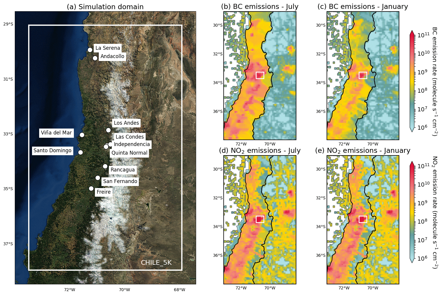
Figure 1 (a) Simulation domain at 5 km spatial resolution centered over Santiago. Locations of interest are designated with white dots. (b) Daily average surface emission rate of black carbon (BC) for July 2015 and (c) January 2015 and  for nitrogen dioxide (NO₂) for (d) July 2015 and (e) January 2015. Map background layer source: Imagery World 2D, ©2009 Esri.

2 Data and methods

2.1 Modeling setup

The chemistry–transport simulations are performed with the Weather Research and Forecasting (WRF) mesoscale numerical weather model from the US National Center for Atmospheric Research (Skamarock et al., 2008) to simulate the meteorological fields and CHIMERE to compute chemistry and transport (Mailler et al., 2017). Anthropogenic emissions are based on the EDGAR HTAP V2 inventory (Janssens-Maenhout et al., 2015). The simulation domain has a 5 km spatial resolution, extending over 200 latitudinal and 100 longitudinal grid points, and is centered on Santiago (white domain CHILE_5K in Fig. 1a). The parameterizations and model configuration used for WRF are presented in Table A1. WRF is applied to 60 vertical levels up to the highest elevation of 50 hPa. Initial and boundary conditions rely on the National Centers for Environmental Prediction (NCEP) final (FNL) analysis data sets, with a $\mathrm{1}{}^{\circ }\times \mathrm{1}{}^{\circ }$ spatial resolution and 6 h temporal resolution, from the Global Forecast System (NCEP, 2000). Land use and orography are extracted from the modified International Geosphere Biosphere Programme (IGBP) Moderate Resolution Imaging Spectroradiometer (MODIS) 20-category database with 30 s resolution (Friedl et al., 2010). CHIMERE is a Eulerian 3-dimensional regional chemistry–transport model, able to reproduce gas-phase chemistry, aerosols formation, transport, and deposition. In this work, the 2017 offline version of CHIMERE is used (Mailler et al., 2017). The model configuration is described in Table A1, with the same horizontal domain as for WRF applied on 30 vertical levels up to 150 hPa. Emissions from the EDGAR HTAP v2 (Emission Database for Global Atmospheric Research Hemispheric Transport of Air Pollution version 2) inventory are downscaled and split in time down to daily/hourly rates following the methodology of Menut et al. (2013). Biogenic emissions fluxes in CHIMERE are computed online using the MEGAN (Model of Emissions of Gases and Aerosols from Nature) model (Guenther et al., 2006). Emission fluxes from the vegetation are based on air temperature, photosynthetic photon flux density, and leaf area index. As an example, an emission map of isoprene (C₅H₈, a VOC involved in the formation of O₃ and secondary organic aerosols), as computed in CHIMERE for a given day in January 2015, is shown in Fig. A1, illustrating the meridional gradient of vegetation cover.

A total of two different simulation periods are investigated to account for summertime and wintertime differences in atmospheric composition and advection dynamics. Summertime hereafter refers to the simulated period from 4 January to 3 February 2015. A 20 d spin-up period between 15 December 2014 and 3 January 2015 is used. Wintertime refers to the simulated period between 1 July and 31 July 2015. A spin-up period from 15 June to 30 June 2015 is applied. For each of these periods, two simulations are performed. The first uses a full emissions inventory, including all emissions within the region, and is henceforth referred to as baseline. The baseline simulation for wintertime is named WB, and the baseline simulation for summertime is denoted as SB. The second simulation corresponds to the case in which the city of Santiago would emit no anthropogenic pollutants. In this regard, all anthropogenic emissions within the area corresponding to the white box in Fig. 1b through 1e are set to zero in the simulation and referred to as the contribution; hence, the designations of WC and SC for the corresponding wintertime and summertime simulations, respectively are used. The difference in simulated concentrations between baseline and contribution runs shows the proportion of pollutants transported to and exported from Santiago. Aerosol feedback on meteorology is not taken into account here, in order to isolate the sensitivity to emission rates only, so that, for a given season, the same WRF fields are used for both emission cases.

Emissions downscaled from the HTAP v2 inventory and input into CHIMERE are shown in Fig. 1b through 1e. The seasonality of BC emissions is clear, given the major role played by residential heating, which takes place mostly in wintertime. Monthly NO₂ emissions are less variable throughout the year, related to the sustained traffic and industrial sources that are nearly constant through time. Figure 1b through 1e also evidences that the city of Santiago (represented with a white box) features the highest emission rates for both pollutants and dominates the signal over the simulation domain. In the continuation, given their relevance for the associated seasons, PM_2.5 in wintertime and O₃ and its precursors in summertime will be considered as the variables of interest, although PM_2.5 in summertime and O₃ in wintertime can be discussed occasionally. PM_2.5 include all primary aerosol species (including dust and sea salt) and secondary organic aerosols but do not incorporate aerosol water.

2.2 Simulation validation

Surface meteorology and pollutants concentrations are validated using data from the automated air quality and meteorology monitoring network of Chile, known as Sistema de Información Nacional de Calidad del Aire (SINCA; https://sinca.mma.gob.cl/index.php/, last access: 1 October 2020). Different stations across central Chile are considered, depending on data availability for the simulated periods (station locations can be found in Fig. 1a). Meteorological vertical profiles in downtown Santiago, for a few days in July 2015, were provided by the Chilean Meteorological Office (Dirección Meteorológica de Chile).

Simulation scores for surface and vertical profile meteorology are gathered in Tables A2 and A3. Biases on daily mean temperature range between −1.23 and 0.31 ^∘C in wintertime, except for the mountainous location of Los Andes, where the bias reaches −3.33 ^∘C. In summertime, the bias is between 0.07 and 0.67 ^∘C. For both periods, correlations on surface temperature vary between 0.7 and 0.89, except for Viña del Mar, where it drops to 0.25 in wintertime and 0.18 in summertime, which can be explained by the proximity of this station to the ocean. The corresponding grid point in the model straddles ocean and land, hence featuring a strong gradient, and, as a result, may not be representative of this coastal city. This remark applies to all meteorological variables at coastal sites. The model shows a negative bias on surface relative humidity, with average mean biases of −15 % to −20 %, but shows fair correlations around 0.8 to 0.9. Surface winds are fairly reproduced, with limited biases and wind gusts well captured, although the correlations can be low for some locations. Figures A2 and A3 compare observed and simulated surface wind distributions for four sites. Summertime shows a good reproduction of wind regimes for all locations, except for a small positive bias on speeds. In wintertime, winds are more variable and follow less clear patterns, so that the model performance is not as good, especially for the coastal locations of La Serena and Santo Domingo. A positive bias on speed is also observed. Most features of the vertical profiles of temperature, relative humidity, and winds are well reproduced, with very good correlations and limited biases for 4 d in winter in downtown Santiago (Tab. A3). On the whole, these statistics give confidence in the ability of the model to produce realistic transport events for both seasons.

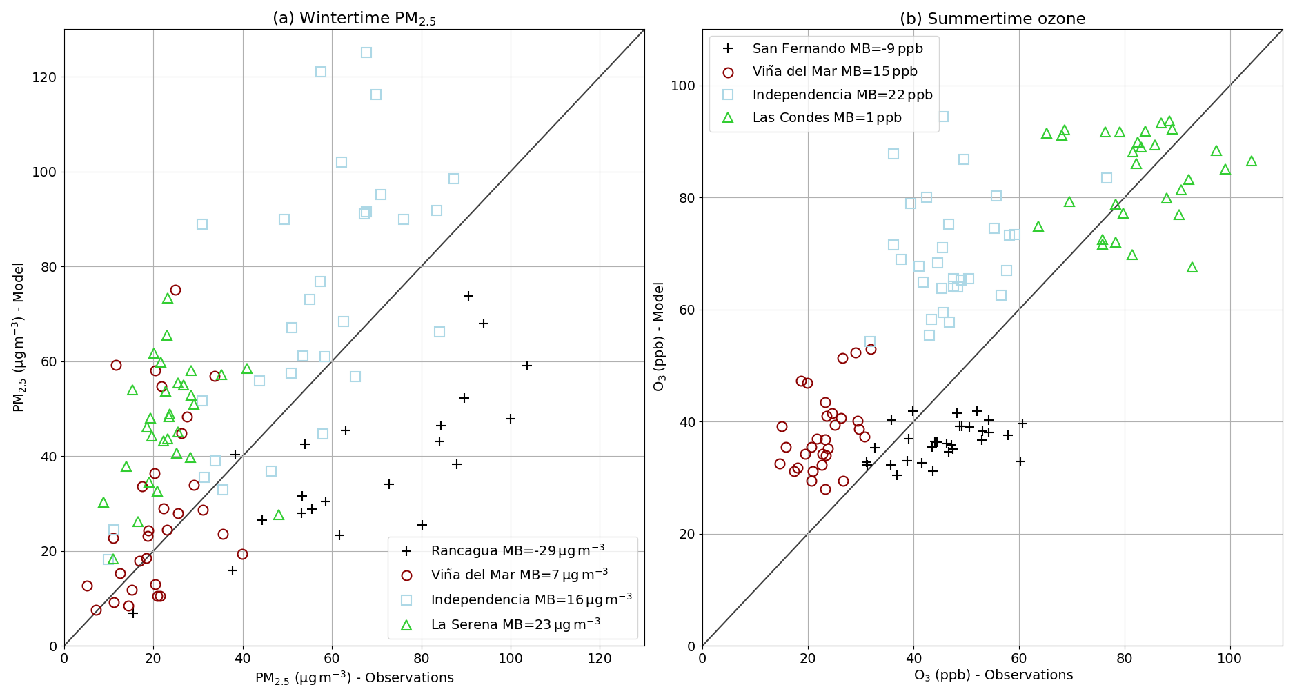
Figure 2 Comparison between observation and simulation for (a) wintertime daily average PM_2.5 concentrations and (b) summertime daily maximum O₃ mixing ratio. Wintertime and summertime correspond to the periods defined in Sect. 2.1, respectively. MB is the mean bias.

Figure 2 shows a scatterplot of the measured and modeled daily mean concentrations of PM_2.5 in wintertime and the daily maximum mixing ratio of O₃ in summertime. For PM_2.5, the simulation performs better for sites far inland with correlations of 0.77 and 0.69 for Rancagua and Independencia, respectively. Correlations for the two coastal sites considered (Viña del Mar and La Serena) are more moderate, with 0.34 and 0.25, respectively. The same issue of straddling grid points explained previously leads to these degraded statistics; while observations at these sites show a chaotic time series, the model produces a smoother diurnal cycle due to the grid point being partially over the ocean. However, for those two sites, biases remain small, while the model systematically underestimates concentrations in Rancagua and slightly overestimates PM_2.5 in Santiago (Independencia). For O₃, the picture is similar, with a good reproduction of daily peaks in summertime. Despite the relatively coarse resolution of the simulation and strong spatial heterogeneity in precursors emissions, limited biases of a few parts per billion (ppb) are obtained on O₃ peaks in summertime, down to only 1 ppb at the most O₃-polluted site of Las Condes (northeastern Santiago). The diurnal cycle of O₃ is also well reproduced, with hourly correlations (not shown here) of 0.67 for Viña del Mar and 0.8 to 0.9 for the three other sites. In parallel, summertime NO_x mixing ratios within the city of Santiago (not shown here) are well captured by the model, with mean biases between 0.05 and 1.23 ppb for three stations in Santiago (Las Condes, Puente Alto in southeastern Santiago, and Independencia), associated with decent hourly correlations between 0.43 and 0.59.

The lack of available measurements for NO_x and VOCs in central Chile hinders the simulation validation regarding these precursors. However, the HTAP inventory has proved reliable for large urban basins in Argentina and Brazil, in terms of the magnitude of VOC emissions (Puliafito et al., 2017; Dominutti et al., 2020), and more generally all across southern South America for NO_x (Huneeus et al., 2020). Consequently, we postulate that emission rates input in the model are appropriate, hence providing adequate chemical regimes when it comes to the simulation of O₃ concentrations. Besides, the known biases of HTAP on these pollutants are critical when it comes to more detailed approaches for policy making, but for the purpose of the present work, having the proper total amount is sufficient as we apply our own downscaling methodology, do not discuss very high-resolution processes, and rely mostly on sensitivity analysis.

In conclusion, PM_2.5 in wintertime and O₃ and its precursors in summertime, the key pollutants for their respective seasons and meteorological conditions, are fairly reproduced by the model for a selection of sites throughout central Chile, which gives confidence in the model outputs that are described and analyzed in the following sections.

3 Results

Hereafter, the well-known general meteorological features generated by the model that provide a first clue regarding the advection of polluted air masses in the region and constitute a frame of reference accounting for the results described in the continuation are discussed.

The semipermanent South Pacific High, centered around (30^∘ S, 110^∘ W), along with the elevated Andes cordillera, are two large-scale drivers of the surface wind systems in central Chile. The persistent high induces high-velocity southwesterlies blowing along the coast during both daytime and nighttime (Fig. 3). These also penetrate deep inland as far as the Andes in summertime during the day, before being blocked by the mountains. On the other side of the Andes, less intensive easterlies coming from Argentina encounter the foothills. Also, the presence of the Andes leads to the development of mountain–valley circulation patterns (e.g., Whiteman, 2000), when the differential heating between narrow valleys and wide plains at the onset and offset of the day lead to the creation of upslope westerlies during the daytime (as seen in Fig. 3b) and a reversal at nighttime with downslope easterlies (Fig. 3d). Although this pattern can be perturbed by clouds or synoptic-scale transient phenomena such as coastal lows, it represents the typical surface wind diurnal cycle for basins along the Andes. From these mean wind fields, the dominant advection pathways of pollutants can be inferred. Polluted air masses are, on average, blown towards the Andes and the north during daytime in summertime and have more complex dynamics in wintertime but also transport northward in general. Deeper and more turbulent planetary boundary layer heights during daytime, as observed in summertime (Fig. 3a), also enable the vertical export of pollutants up into the free troposphere (FT) where they can be advected farther, while wintertime shallower boundary layers (Fig. 3b) imply more stagnation of air masses.

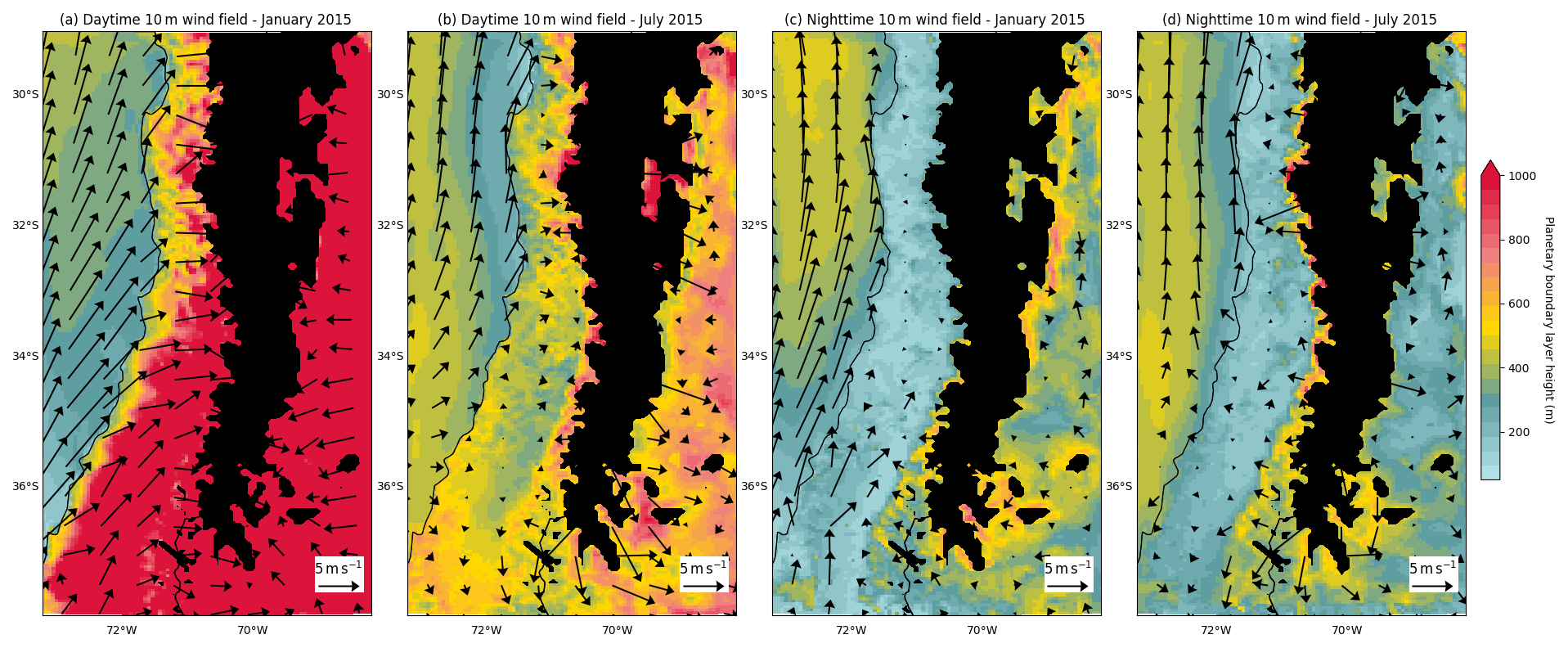
Figure 3 Average 10 m wind field (arrows) and planetary boundary layer height (color map) simulated by WRF (a) during the daytime in January 2015 and (b) July 2015 and during nighttime in (c) January 2015 and (d) July 2015. Black areas show grid points with an elevation in excess of 2000 $\mathrm{m}\mathrm{a}.\mathrm{s}.\mathrm{l}.$

3.1 Impact of emissions from Santiago on regional atmospheric composition

3.1.1 Wintertime PM_2.5

Consistent with the mean wind fields and emission rates of pollutants in central Chile discussed previously, anthropogenic emissions in the city of Santiago significantly influence surface atmospheric composition over a large region, over land, the Andes, and the Pacific Ocean. The following results are based on the analysis of sensitivity to emissions from Santiago described in Sect. 2.1: the difference between the simulation with (baseline case) and without (contribution case) emissions from Santiago yields their contribution to atmospheric composition over the domain. Figure 4a and b show the average wintertime PM_2.5 plume (absolute and relative, respectively) attributable to emissions from the capital city area. The direct western vicinity of the Santiago basin receives, on average, 5 to 15 µg m⁻³ coming from the capital city, a few tens of kilometers from the source, corresponding to more than 30 % of the signal simulated in the baseline scenario for this area. At the scale of hundreds of kilometers, the export drops to a few µg m⁻³, corresponding to 5 % to 20 %. It is worth noting that the relative contribution of emissions from Santiago remains greater than 5 % on an area as large as more than 8^∘ meridionally and 3^∘ zonally, hence stressing the significant impact of the capital city on atmospheric composition for the whole region (Fig. 4b). In particular, the southern part of the plume is transported over the Andes down to Argentina, with a large spread of several degrees of longitude, whereas the northern part extends mostly along the coast in a narrower manner and transports as far as the boundary of the simulation domain.

More specifically, urban areas along the north–south axis of Santiago (Curicó, San Fernando, Rancagua, and Los Andes in Fig. 4a) receive 1 to 2 µg m⁻³ from Santiago on an hourly basis on average, corresponding to 4 % to 8 % of the baseline concentrations (Fig. 4c). Sporadically, up to more than 20 µg m⁻³ in Rancagua and 9 µg m⁻³ in San Fernando, Curicó and Los Andes can be attributed to emissions from Santiago. These significant contributions likely lead to alert thresholds being crossed for some hours in these cities.

On the eastern side of the Santiago basin is the Andes cordillera. We examine the contribution of Santiago emissions in a mountain locality (San Gabriel; 1250 $\mathrm{m}\mathrm{a}.\mathrm{s}.\mathrm{l}.$) and a summit (Maipo volcano; 5264 $\mathrm{m}\mathrm{a}.\mathrm{s}.\mathrm{l}.$) along the Maipo canyon, southeast of Santiago. We find that for San Gabriel, 34 % (1 µg m⁻³) of PM_2.5, on average, is transported from the urban basin. This is consistent with the mountain–valley circulation patterns aforementioned, leading to the intrusion of urban air masses deep into the canyon (Lapere et al., 2021b). We acknowledge that the estimate of 34 % is probably larger than reality, since the HTAP inventory does not properly capture local emissions in the village of San Gabriel, which likely dominate the signal, especially with wood burning for residential heating being largely used in such villages in wintertime. In the Maipo volcano area, a small contribution in absolute value is found (less than 0.5 µg m⁻³), although it can reach up to more than 2 µg m⁻³ occasionally, but this corresponds to 20 % of the signal there on average. This area is covered in snow during wintertime, so that, despite the small magnitude of the import of PM_2.5, it can lead to significant radiative effects when deposited (Rowe et al., 2019), especially given the large fraction of BC in PM_2.5 emitted in Santiago, which is around 15 % according to the HTAP emissions inventory.

The Viña del Mar–Valparaíso area is the second-largest populated region of Chile, located on the coast of central Chile, approximately 100 km west of Santiago. In wintertime, it is downwind of Santiago, which leads to an average import of particulate matter from the capital city of 3 µg m⁻³ (18 %) and sporadically up to 18 µg m⁻³. Again, air quality in this urban area is worsened by export from Santiago by a significant share. Further north, at the location of La Serena, which also suffers from bad air quality in wintertime, the contribution of Santiago emissions is more moderate but still remains significant in absolute value although its contribution is only 1 %.

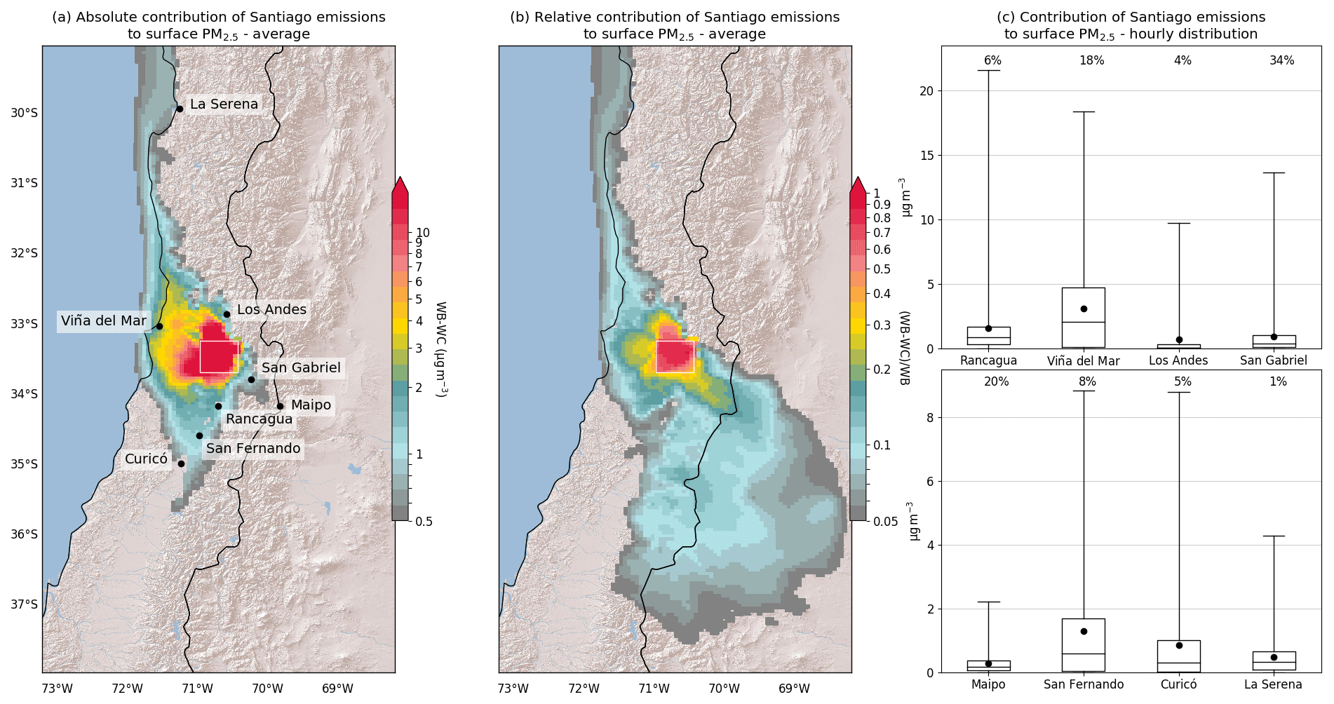
Figure 4 (a) Average ground-level PM_2.5 concentration difference between WB (winter baseline case) and WC (winter contribution case) yielding the Santiago emissions contribution. Concentrations in excess of 0.5 µg m⁻³ are displayed. The white box shows the area in which emissions are set to zero in WC. Panel (b) is the same as (a) in terms of the relative contribution, i.e., (WB-WC)/WB. Contributions in excess of 5 % are displayed. (c) Distribution of Santiago emissions contribution to hourly PM_2.5 concentration at several sites across central Chile; horizontal lines are quartiles, whiskers show minimum and maximum, and the dots are the means. All figures are based on hourly concentrations and are for wintertime 2015. In panels (a) and (b), only grid points at which the distribution of concentrations in scenario WC is different than in scenario WB at the 90 % level, based on a t test, are shown. Map background layer source: World Shaded Relief, ©2009 Esri.

3.1.2 Summertime O₃

In summertime, except for PM_2.5 emitted by biomass burning events (not considered here), O₃ is the pollutant raising concern. Combined significant emissions of NO_x and VOCs are required, in the presence of sunlight, to generate high mixing ratios of O₃. However, a lot of nonlinearities are involved in the tropospheric O₃ cycle, so the sensitivity to its precursors emissions is not straightforward. For instance, imbalances in the ratio of NO_x and VOCs decrease O₃ formation. Given the crucial role of photolysis in O₃ formation, it features a strong diurnal cycle, with levels coming back to low values at night. Thus, the important variable for determining whether O₃ pollution is high is its daily maximum mixing ratio, which we will mostly focus upon hereafter.

Figure 5a shows the average of maximum hourly O₃ mixing ratio at ground-level observed each day in the baseline case (SB). In the baseline scenario, O₃ is mostly found at harmful levels in the vicinity of Santiago, mainly on its eastern side. Again, mountain–valley circulation accounts for this observation; afternoon westerlies blow O₃ precursors, present in large amounts in urban air masses, towards the Andes. The NO_x lifetime is a few hours at most, depending on the reactivity of VOCs and NO₂ density (e.g., Laughner and Cohen, 2019), while most VOCs have an atmospheric lifetime of several days (e.g., Monod et al., 2001) so that, on the way, NO_x are consumed more than VOCs. Consequently, while urban air is mostly a NO_x-rich environment, precursors ratios become more balanced, along with the export, to create more favorable conditions for O₃ formation on reaching less urbanized areas. Such a mechanism has been observed for Paris and its suburbs, for instance (e.g., Menut et al., 2000). Export by easterlies occurs less frequently and mostly at night when O₃ cannot be created due to lack of sunlight, which is why the rural area west of Santiago shows smaller O₃ maxima. This mechanism explains the large concentrations of O₃ mostly found east of Santiago. Except for the center part of the domain, where average daily maxima reach more than 100 ppb, O₃ pollution is less concerning elsewhere in central Chile, where it ranges between 10 and 35 ppb.

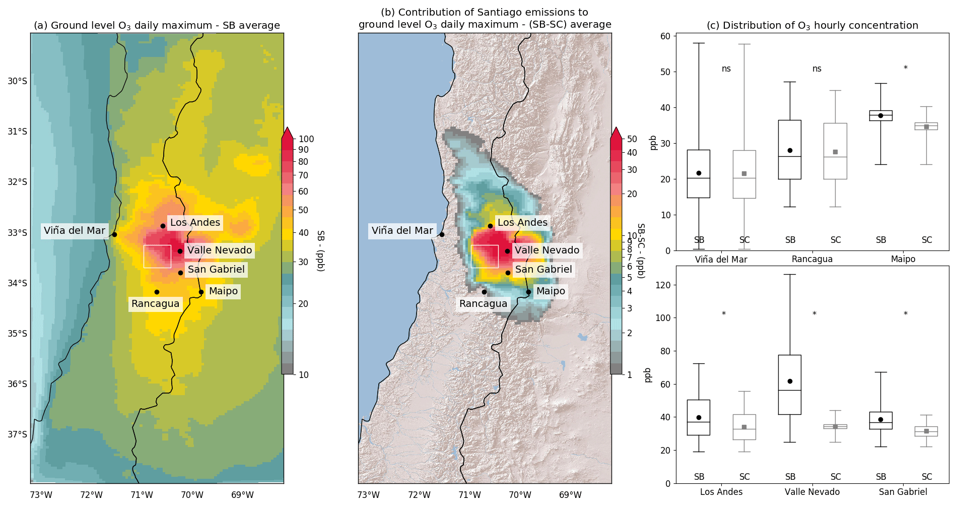
Figure 5 (a) Ground-level O₃ average daily maximum of hourly mixing ratio in scenario SB. (b) Difference between SB and SC ground-level O₃ average daily maximum of the hourly mixing ratio. (c) Distribution of hourly O₃ mixing ratio at six locations in scenarios SB (black) and SC (gray); horizontal lines are quartiles, whiskers show the minimum and maximum, and dots show the average; ns indicates that the distribution in the SB and SC scenarios cannot be distinguished at the 90 % level based on a t test. The asterisk (^*) indicates that they are different at the 99 % level, based on that same t test. Map background layer source: World Shaded Relief, ©2009 Esri.

Figure 5b shows the decrease in O₃ daily maxima induced by eliminating emissions of the Santiago basin. The spatial pattern is again consistent with the mechanism introduced previously; emissions of precursors from Santiago are the main origin for O₃ formation in the Andes and north of the city, with a reduction of more than 50 ppb in the daily maxima over this area when the capital city no longer emits pollutants.

More specifically, the northern city of Los Andes shows a decrease in its daily maxima by 15 ppb on average (Fig. 5b), while the average mixing ratio drops from 40 to 33 ppb (Fig. 5c). Similarly, at the ski resort site of Valle Nevado (3000 $\mathrm{m}\mathrm{a}.\mathrm{s}.\mathrm{l}.$), which shows concerning levels of more than 60 ppb of O₃ on average in the baseline case, the mixing ratio drops to an almost constant value of 33 ppb and does not go above 43 ppb. This points to O₃ in Valle Nevado being almost exclusively attributable to Santiago emissions. To a lesser extent, the location of San Gabriel shows the same trend, although the still wide distribution in scenario SC advocates for a significant contribution of local sources as well. The impact of Santiago emissions in the vicinity of the Maipo summit is small but remains significant with a decrease by 4 ppb of the daily maxima and average mixing ratios. Given the nature of the locations of Valle Nevado and Maipo, the narrow distribution of O₃ hourly mixing ratio, averaging at 33 ppb and ranging between 25 and 40 ppb, recovered in scenario SC for those sites is indicative of the background concentration for the region, i.e., the distribution of a O₃ mixing ratio that would be observed at a site not influenced by anthropogenic emissions.

On the other hand, the western and southern areas adjacent to Santiago are barely sensitive to its emissions. In Fig. 5c, the distribution of hourly O₃ mixing ratio at Viña del Mar and Rancagua is nearly the same in both scenarios, except for the maximum at Rancagua, which is a few parts per billion less in scenario SC than scenario SB. For those two locations, the difference in O₃ distribution with or without Santiago emissions is not significant at the 90 % level, while, for all other locations, distributions are significantly different at the 99 % level.

3.2 Contribution of regional emissions to atmospheric composition in Santiago

Similar to the previous approach, we can, in a symmetric manner, deduce the contribution of transport from remote sources to atmospheric composition in the city of Santiago. This is achieved by looking at concentrations in the contribution case that exclusively originate from nonlocal sources. Hereafter, the analysis focuses again on PM_2.5 in wintertime and O₃ in summertime.

3.2.1 Wintertime PM_2.5

Figure 4b indicated that local emissions largely dominate the wintertime PM_2.5 signal for Santiago, with 50 % to 100 % of the mean surface concentration of PM_2.5 originating locally within the white box. Nevertheless, the contribution of transport is also significant, although heterogeneous, in Santiago. Figure 6a shows that, in the baseline scenario, the northern and western parts of Santiago feature higher levels of PM_2.5, with average concentrations ranging between 30 and 100 µg m⁻³ for the whole metropolis. In the contribution scenario (Fig. 6b), this pattern is partly recovered, with a smoother gradient from west to east. The underlying conclusion is twofold. First, the transport of pollutants in Santiago mostly comes from the west, which is consistent with the presence of the mountain range in the east not featuring many sources of pollution and the dominant westerly daytime wind direction in wintertime. Second, the districts of Santiago facing the worst air quality are also the ones where the transport of pollutants is larger.

However, the differing patterns between Fig. 6a and 6b also shows that local sources in these districts are also stronger. If emissions were similar, the observed gradient in WB would be closer to that in WC. Consistently with this observed westward gradient, we define 5 zones of interest, comprising 6 grid points each along a meridional axis (rectangles and dots in Fig. 6b). This arrangement ensures that most of the city is covered while maintaining the west-east variability. For each zone we look at the distribution of PM_2.5, averaged over the 6 grid points, in scenarios WB and WB–WC (Fig. 6c) and WC (Fig. 6d). When averaged meridionally, the westward gradient is also obtained in scenario WB and conserved when the contribution of transport is substracted (WB vs. WB–WC in Fig. 6c). On average, the contribution of transport to PM_2.5 concentration ranges between 10 µg m⁻³ for the westernmost area and 5 µg m⁻³ for the easternmost part, with a monotonic spatial variation (Fig. 6d). However, this amount always corresponds to between 13 % and 15 % of the WB concentrations. This number is well in line with Barraza et al. (2017), who found 9 % of PM_2.5 in Santiago coming from coastal sources for the period 2011–2012. It is worth noting that, given the observed westward gradient, we also recover that coastal sources are likely the main contributor to imported PM_2.5. Again, transport is larger in western Santiago, and can sporadically reach up to 30 µg m⁻³, but it does not constitute a greater share than in the east.

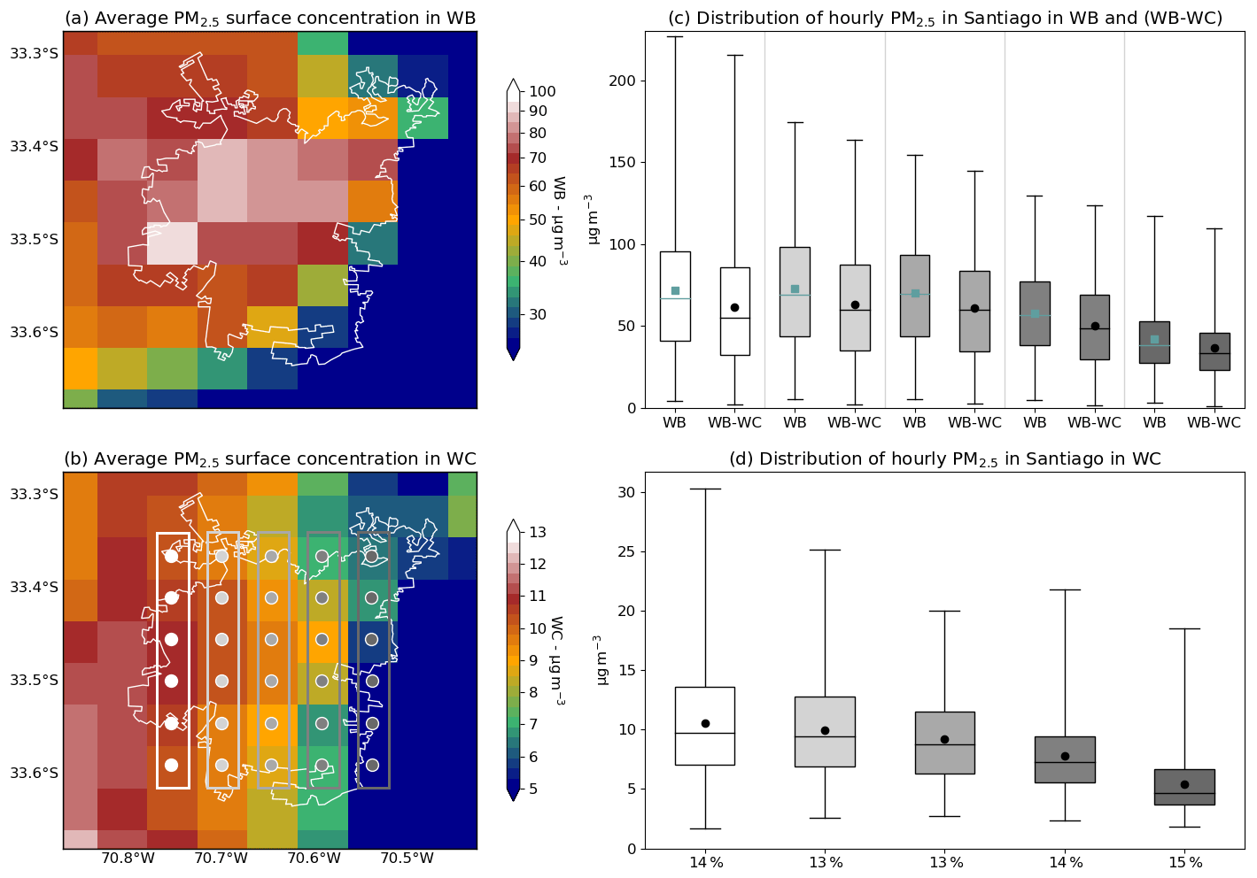
Figure 6 (a) Average ground-level PM_2.5 concentration in scenario WB. The white contour shows the boundaries of Santiago. Panel (b) is the same as panel (a) for scenario WC. (c) Distribution of hourly PM_2.5 surface concentration in WB and WB–WC. Boxes show the average, median, minimum, maximum, and first and third quartiles. Shades of gray correspond to the zones defined in (b) on which an average is made. Panel (d) is the same as panel (c) for scenario WC. Percentages indicate the relative average contribution of transport.

This averaged picture provides a first clue as to the main origin of PM_2.5 transport in Santiago, but the picture can be refined by looking at the joint distribution of hourly wind direction and PM_2.5 concentrations shown in Fig. 7. At the selected southeastern location, mostly clean air comes from the east, i.e., from the Andes, where pollutant sources are scarce (less than 5 µg m⁻³ for almost every hour), while winds blowing from the southwest can transport concentrations as high as 20 µg m⁻³ or more for some hours, pointing to the southern cities of Rancagua (34.2^∘ S, 70.7^∘ W) or San Fernando (34.6^∘ S, 71^∘ W) mentioned previously or the southwestern urban location of Melipilla (33.6^∘ S, 71.2^∘ W). At the northeastern site, winds mainly come from the north, where only a handful of urban areas are found, hence leading to a transport seldom exceeding 10 µg m⁻³. In the center of the metropolis, winds are either southwesterlies (from the Rancagua and Melipilla areas) or northwesterlies (from the Viña del Mar–Valparaíso area), with both cases leading to similar amounts of imported PM_2.5 mostly above 10 µg m⁻³, i.e., above average. The picture is similar for the northwestern and southwestern sites, although wind directions are shifted.

In the northwest, center, and northeast, the dominant wind directions also coincide with higher maximum relative contributions of transport over the period along these directions (black diamonds in Fig. 7). Sporadically, significant transport events can also come from less frequently observed directions. The maximum relative contribution obtained for the northwestern point, when winds are from north-northeast, is 75 %, for example, while such winds occur less than 1 % of the time. For southwestern and southeastern locations, these maximum relative transport episodes are observed when winds blow from the south, in particular in the southeast, where it can reach up to 100 %.

Figure 7 Joint distribution of hourly wind direction (length of the bar gives the frequency of the corresponding wind direction) and PM_2.5 concentration (color map) in scenario WC for five locations in Santiago. Black diamonds show the maximum relative contribution of transport (i.e., WC or WB) for each wind direction bin (note – the scale is the wind frequency scale multiplied by 5; i.e., 0.20 is actually 1.0). The bottom center map shows the location of the considered grid points. Map background layer source: Imagery World 2D, © 2009 Esri.

In summary, wintertime PM_2.5 concentrations in Santiago are significantly (5 to 10 µg m⁻³ on average) and always (at least 1 µg m⁻³ for every hour) affected by transport with identifiable origins, and although the different districts are not equally affected in absolute value, the relative burden of imported particulate matter is equivalent.

3.2.2 Summertime O₃

Based on the same approach, we find that the summertime transport of NO_x within the Santiago basin never exceeds 0.5 ppb, while average values in the SB scenario are between 5 and 40 ppb, with a similar westward gradient as observed for PM_2.5 (not shown here). At the 90 % level, NO_x transport is, thus, not significant. Similarly, the transport of VOC is homogeneous over the whole basin at 2 ppb on average, while it is between 20 and 60 ppb in the SB scenario, which is again not significant at the 90 % level. Santiago is, thus, not affected by the transport of O₃ precursors.

However, the picture within Santiago city in the SB and SC scenarios is complex. In the baseline scenario, the eastern area of Santiago is more affected by O₃ pollution compared to the western area (Fig. 8a and c), consistent with observations and the literature (e.g., Menares et al., 2020), due to a more balanced $\mathrm{VOC}/{\mathrm{NO}}_{\mathit{\text{x}}}$ ratio than in the western area. At Independencia (central Santiago), the $\mathrm{VOC}/{\mathrm{NO}}_{\mathit{\text{x}}}$ ratio of emissions is between 1:1 and 2:1 on average. Contrarily, at Las Condes (eastern Santiago) the $\mathrm{VOC}/{\mathrm{NO}}_{\mathit{\text{x}}}$ ratio of emissions is around 6:1 on average in the baseline case (not shown here). A typical O₃ formation ridge line of the $\mathrm{VOC}/{\mathrm{NO}}_{\mathit{\text{x}}}$ concentration ratio in urban areas is around 6:1 to 8:1 (e.g., National Research Council, 1991; Sillman, 1999), so Independencia features a VOC-limited regime, while Las Condes features a balanced regime favorable to O₃ formation, hence the larger amounts found at the latter location.

Figure 8b shows the consequences, on the O₃ surface mixing ratio, of eliminating emissions within Santiago. Given the configuration described previously, in the baseline case, the VOC-limited districts of western Santiago feature mixing ratios well below the background level due to the titration of O₃ by excess quantities of NO_x, while the eastern districts feature mixing ratios above the atmospheric background level due to excess O₃ formation under a favorable regime. As a result of shutting off emissions, given that there is no import of precursors, as evidenced above, the whole area is set to the background O₃ level of around 30 ppb described in Sect. 3.1.2, since there is no influence of anthropogenic pollutants anymore. Therefore, this corresponds to an increase in O₃ in western Santiago and a decrease in O₃ in eastern Santiago, thus explaining the dipole obtained in Fig. 8b. Such an evolution is also clear in the evolution of the distribution of hourly O₃ mixing ratios across the city between scenarios SB and SC (Fig. 8c). While the distribution is shifted towards larger mixing ratios when going eastward in scenario SB, all distributions are equal (significant at the 99 % level) in scenario SC. The leveling of mixing ratios, with no gradient across the city in scenario SC, constitutes additional evidence that O₃ in Santiago is not affected by long-range transport, otherwise heterogeneous patterns similar to what is observed in Fig. 6b would be obtained.

Figure 8 (a) Average O₃ mixing ratio at ground level in scenario SB in Santiago. Panel (b) is the same as panel (a) for scenario SC–SB. (c) Distribution of hourly O₃ surface mixing ratio in scenarios SB and SC. Boxes show the average, median, minimum, maximum, and first and third quartiles. Shades of gray correspond to the zones defined in (b) on which an average is made.

3.3 Advection processes

As discussed around Fig. 3 and observed in Figs. 4 and 5, advection patterns of pollutants differ between wintertime and summertime. So far, the analyses focused on surface fields, but processes along the vertical direction drive these differences. Figure 9 shows an average latitude and altitude transect, along central Chile, of winds, afternoon mixing layer height, and pollutants concentrations for the corresponding season in the baseline scenario and in the Santiago isolated contribution case. In wintertime (Fig. 9b and 9c), the boundary layer (solid white line) is shallow, and average winds in the FT are strong, consistent with the observed semipermanent inversion layer in the region. As a result, the PM_2.5 emitted in large amounts mostly remain trapped within this shallow mixing layer. Injection of polluted air masses into the lower FT can also occur through mountain venting, as described in Lapere et al. (2021b), explaining why residual concentrations of 1 to 5 µg m⁻³ are observed higher up in the baseline and contribution scenarios at the latitude of Santiago (Fig. 9b and c). Nevertheless, the long-range export of PM_2.5 from Santiago observed in Fig. 4 is mainly driven by advection within the boundary layer, close to the ground, by weak winds, as evidenced by Fig. 9c. Except for a shallow residual layer located above the average afternoon boundary layer, pollutants emitted from Santiago remain within it along the transect from Santiago to Viña del Mar. The pattern changes when reaching the seashore, however, with significant wind shears lifting the PM_2.5 layer above the mixing layer (rightmost part in Fig. 9c), where intense southerlies are found, thus explaining the wide northward extent of Santiago contribution.

In this wintertime averaged picture, the patterns underlying the largest transport events are not obvious. In order to identify these advection patterns, four clusters are designed corresponding to episodes of transport from Santiago to the south (Rancagua), from Santiago to the northwest (Viña del Mar), into Santiago from the south, and into Santiago from the northwest. In the case of transport into Santiago, passive aerosol tracers emitted in the model at the locations corresponding to Rancagua and Viña del Mar are used to discriminate the main direction of origin. The composite of these episodes is defined as the hours when the PM_2.5 (or tracer) contribution to concentration is greater than or equal to its 90th percentile over the studied period. The meteorological conditions during these particular hours are then compared to the average for the whole period in order to compute anomalies in the surface wind and pressure fields. Figure A4 shows that southward transport events are associated with lower than average surface pressure by 1 to 3 hPa and large northerly anomalies over most of the wind field and, in particular, in the corridor between Santiago and Rancagua. Conversely, northwestward export is associated with positive anomalies in surface pressure and a southerly anomaly in surface winds combined with easterly anomaly in the corridor between Santiago and Viña del Mar. The two aforementioned corridors are shown as the topographic contours in Fig. A4. These variations are related to the dynamics of the Southeast Pacific High, located near (35^∘ S, 110^∘ W); a weakening or southward and/or westward displacement of the anticyclone lead to the anomalies observed in Fig. A4a, while an opposite displacement leads to a situation similar to that in Fig. A4b. Consistently, transport events into Santiago are related to symmetrical patterns (not shown here), with transport from the northwest featuring similar anomalies to those in Fig. A4a and transport from the south originating in the same anomalies as those in Fig. A4b.

Interestingly, the summertime transect of O₃ shows a sharp maximum near the latitude of Santiago occurring several hundred meters above the ground. Figure 9d shows the formation of an O₃ bubble of more than 50 ppb on average, i.e., 15 ppb above the 35 ppb background mixing ratio observed in scenario SB (dominant yellow and/or green levels in altitude in Fig. 9d), around 33^∘ S, i.e., slightly north of Santiago, above the planetary boundary layer, extending between 1.5 and 3 km altitudes. This additional O₃ plume is mostly attributable to emissions of precursors in Santiago that account for more than 15 ppb of O₃ on average at the location of the bubble (Fig. 9e), i.e., the background level exceedance. Thus, despite a relatively limited area in which precursors from Santiago affect O₃ formation near the ground (Fig. 5b), their impact on the vertical profile is more dramatic. The process underlying the formation of this significant O₃ bubble clearly departing from the background is discussed hereafter. It is also worth noting that even though export of O₃ close to the surface is limited (Fig. 5b), it is more widespread higher up, with a residual layer originating from Santiago emissions of a few parts per billion extending 2 km vertically and transporting northward in the FT along more than 200 km (Fig. 9e).

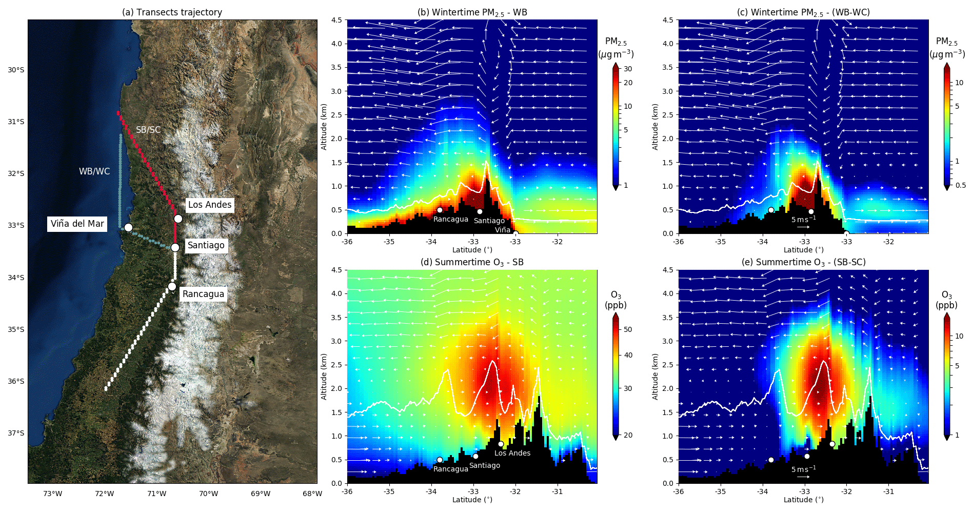
Figure 9 (a) Trajectory of the considered latitude and altitude transects and main locations along the way. The white dotted line up to Santiago is common for both seasons, the blue dotted line is for wintertime, and the red dotted line is for summertime. Values in the transects are not zonally averaged; they correspond to the grid points represented with dots. (b) Simulated PM_2.5 concentrations (color map), wind (white arrows), afternoon boundary layer (white solid line), and terrain elevation (black area) along the white and blue transect; average for wintertime 2015 for the WB scenario. Panel (c) is the same as panel (b) for scenarios WB–WC. (d) Simulated O₃ mixing ratios (color map), wind (white arrows), afternoon boundary layer (white solid line), and terrain elevation (black area) are shown along the white and red transect; average for summertime 2015 for the SB scenario. Panel (e) is the same as panel (d) for scenarios SB–SC. Map background layer source: Imagery World 2D, © 2009 Esri.

Given the proximity of the Andes cordillera to the Santiago basin, the formation of the aforementioned O₃ bubble finds its origin in the mountain–valley circulation and the associated mountain venting mechanism. Daytime upslope winds, strong in summertime, lift polluted air masses from the atmospheric boundary layer (ABL) over Santiago into the lower FT, possibly above another location, depending on the FT wind direction. McKendry and Lundgren (2000) and Lu and Turco (1996) find that this process is a net sink for boundary layer O₃ in British Columbia and the Los Angeles basin, respectively. Henne et al. (2005) find that the effect of venting in an Alpine environment on FT O₃ concentrations strongly depends on initial mixing ratios within the vented ABL, with either net production, if ABL mixing ratios of O₃ are high (urban valleys), or net loss, if they are low (remote valleys). However, our study case falls into none of the aforementioned categories. Such a bubble of O₃, detached from the ground, with a mixing ratio much higher than at ground level is not found in the literature to our knowledge. More moderate injections, with O₃ mixing ratios lower than or similar to surface levels are usually observed. In our case, we find that the venting of precursors from the Santiago polluted ABL leads to the net production of large quantities of O₃ in the FT, larger than at the surface. Schematically, there is a larger export of VOCs than NO_x in the FT (Fig. A5a and b), which makes for a balanced chemical regime (below 0.5 is NO_x limited; above 0.5 is NO_x rich) at around 0.5 at 2 km altitude, while the regime is close to 1 near the surface and, hence, unfavorable to O₃ production along the whole transect, due to dominant urban NO_x emissions (Fig. A5c). Also, the export of peroxyacetyl nitrate (PAN), which is a NO_x carrier, into the FT contributes to enhanced O₃ formation (Fig. A5d).

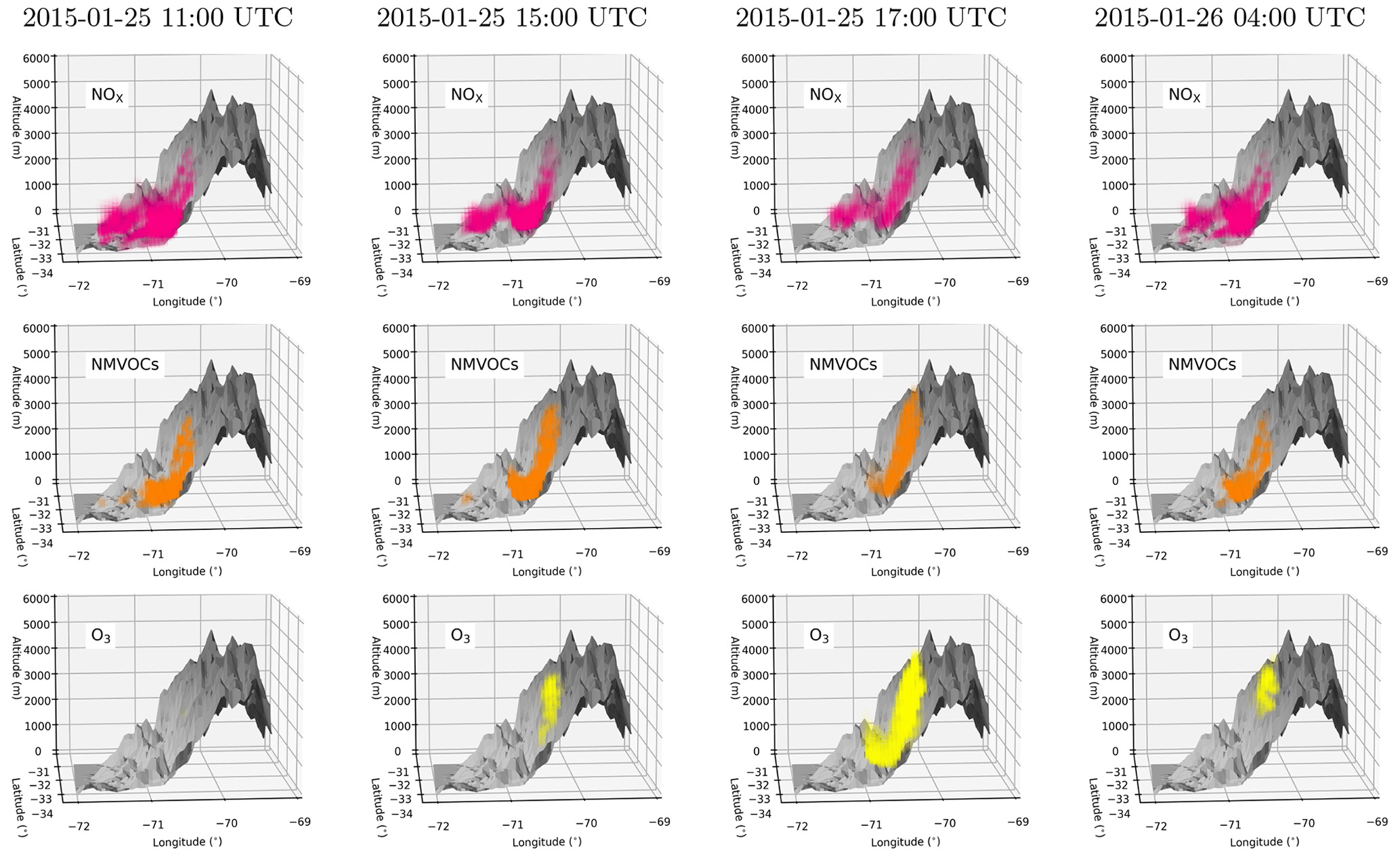
Figure 10 Cycle of NO_x (top), NMVOC (middle) and O₃ (bottom) venting in the vicinity of Santiago for a typical day in January 2015. Hourly mixing ratios in excess of 2, 20, and 60 ppb are shown, respectively. Each panel shows a 3-D view from a longitudinal perspective. Gray surfaces represent the terrain topography. Times for Santiago are universal coordinated time (UTC−3) for this period.

Figure 10 further sheds light on the dynamics of this mechanism. Early in the day, at 11:00 universal coordinated time (UTC−3 in Chile in summertime), both NO_x and NMVOC (non-methane VOC) are highly concentrated near the ground (morning peak of emissions from traffic), and start ascending the Andean foothills, but no O₃ is formed in the region given that sunlight is not intense yet (leftmost column in Fig. 10). A few hours later, at 12:00 local time (LT; 15:00 UTC), the precursors have a similar distribution as in early morning, but the photolysis starts taking place, and O₃ is created at the top of the precursors plume, well above the ground.

There are two factors explaining why O₃ is not formed near the source of precursors. First, given the urban environment of the basin, NO_x are emitted in large quantities so that the VOC/NO_x ratio is adverse to neutral, and O₃ is formed in small amounts (see the related discussion in Sect. 3.2.2). But NO_x have a lifetime that is much shorter than most VOCs (e.g., Monod et al., 2001; Laughner and Cohen, 2019), and when the polluted air parcels are lifted up, the ratio becomes more balanced as NO_x is consumed closer to the ground. Due to these asymmetric lifetimes and, hence, export, at some point on the vertical profile the ratio becomes favorable (Fig. A5c), and O₃ is formed in large quantities. The second factor comes from the increase in photolysis rates with altitude. Several hundred meters above the ground, near or above the mixing layer, photolysis rates of NO₂ are much faster than at ground level (e.g., Pfister et al., 2000), hence favoring the formation of O₃ with all other things being equal. In our simulation, on average, the photolysis of NO₂ is 20 % faster 1000 m above ground than at the surface. Also, Fig. 9d shows that, at the point where the O₃ plume is denser, winds are weak to null on average, so that precursors stagnate, again allowing for more O₃ creation.

At 14:00 LT (17:00 UTC), the vertical export of precursors is even more important due to the maximum development of the deep mixing layer and the full intensity of upslope winds, with two main consequences. First, NO_x levels in Santiago decrease compared to VOCs due to vertical export earlier in the day, leading to a more favorable ratio, and O₃ starts forming in the urban basin near the surface. Thus, ventilation of precursors possibly increases O₃ surface concentration in Santiago. Second, the O₃ plume in the lower FT intensifies and extends up to an altitude of 4 km. Finally, at 01:00 LT (04:00 UTC) the next day, the return of a shallower mixing layer and the accumulation of evening traffic emissions make precursors concentrations larger near the ground again. With the Sun being down, O₃ stops forming, but, given the large amounts created during the day, a residual plume remains around 1 km above ground. In parallel, as the winds along the transect are mostly southerlies, the O₃ plume ends up approximately 50 km north of the Santiago basin.

4 Discussion

Figure 2 revealed moderate biases in the modeled concentrations of PM_2.5 and O₃ compared to downtown Santiago observations. These discrepancies can stem from (i) the relatively coarse resolution of the simulation compared to the heterogeneity of pollution at the scale of Santiago city; (ii) the static nature of the emissions inventory as of 2010, while air pollution follows a decreasing trend in Santiago, hence accounting for the overestimation of primary emissions by the model; and (iii) a slight negative bias in the representation of mixing layer height in the simulation contributing to over-concentrated particulate matter. In practice, a combination of the three is likely at play. Although the processes of transport evidenced in this study are not sensitive to such biases, quantitative conclusions can depend on them to some extent. In particular, if case (ii) dominates the discrepancy on PM_2.5, biases in emissions can be asymmetric between Santiago and other locations, given that the trends recorded since 2010 are probably not identical (the model in Rancagua is negatively biased, for example). In that case, an overestimation of the relative contribution of Santiago emissions at these locations could be found. If the bias mostly comes from reason (i) or (iii), the quantification should be resilient. The Santiago source is considered at a larger-scale than downtown so that local discrepancies should compensate over the whole area (case i), and in case (iii), the bias should concern most locations, and does not have an influence on emissions, and, therefore, should not modify relative contributions. Regarding the biases on O₃ mixing ratio, case (i) is most likely to be the underlying bias, as levels are better reproduced in the eastern part of Santiago (Las Condes), thus pointing to localized disagreements. More generally, we cannot exclude possible shortcomings of the chemistry–transport model itself to explain the disagreement. Although CHIMERE has been systematically evaluated over Europe, it has not been extensively used over South America so far. In that case, identifying the causes and consequences is more complex.

Only one particular month per season for one particular year is analyzed here. Whether the results presented can be extrapolated with a climatological relevance is not straightforward. Climate variability modes such as the El Niño–Southern Oscillation (ENSO), for instance, can lead to interannual changes in circulation and meteorology at the scale of central Chile. In particular, El Niño phases are related to above-average rainfall in the region in winter (Montecinos and Aceituno, 2003), hence leading to more frequent scavenging of particulate matter that may imply less regional transport. La Niña years do the opposite, with a drier winter. In addition, ENSO affects the southeastern Pacific anticyclone, thus modulating wind speeds along the shore of central Chile (Rahn and Garreaud, 2014). Weaker winds are observed in case of El Niño so that northward transport likely decreases as a consequence. Again, the opposite can be said for La Niña. ENSO also modulates the severity of the fire season in summertime in the region (Urrutia-Jalabert et al., 2018). However, as pointed out in Sect. 1, wildfires are not taken into account in our simulation design so that our findings are resilient to this variability. Speculating on the impacts regarding our results of the ENSO-related synoptic-scale variability of atmospheric circulation is even more complex in the context of the last decade, as the ENSO teleconnection in central Chile is weak for that period (Garreaud et al., 2020). However, although our quantitative conclusions may not exactly hold for other years, the underlying processes described remain valid, particularly when it comes to mountain–valley circulation, which is radiatively driven. Variations in primary pollutants and precursors emissions, wintertime precipitation, and cloud cover may affect our results, but we do not expect new processes to take place, evidenced processes to stop, or magnitudes to change entirely. Indeed, the year 2015 was chosen because it recorded no particular extreme pollution event, and it corresponds to a period of weak teleconnection between ENSO phases and the Chilean climate. In addition, primary emissions in the model are not weather dependent, and the inventory is static as of 2010, meaning the fluxes of primary anthropogenic emissions would be equal for any simulated year. Therefore, the picture provided by this study is statistically representative of average summer and winter months, despite not being directly extendable.

Section 3.3 evidences the asymmetric vertical ventilation of pollutants, such as NO_x and VOC, and their role in the formation of an O₃-persistent plume. Given the quite unique combination of very high emission rates and close proximity of steep elevated orography featured in the Santiago basin, it is unclear, based on the literature, whether this venting is expected to improve or worsen O₃ pollution at the surface level in the city. To some extent, this asymmetric venting of precursors is similar to the sensitivity analysis performed in Sect. 3.2, leading to a change in precursors ratios, except for the magnitude of the variation in pollutants emissions. Thus, one could extrapolate and expect an increase (decrease, respectively) in O₃ mixing ratio in the western (eastern, respectively) districts due to this daily occurring export of pollutants, compared to a situation where air masses would stagnate. However, there are too many nonlinear processes involved to be affirmative on this point.

In addition to being a pollutant, tropospheric O₃ is a strong greenhouse gas, estimated to contribute between 0.2 and 0.6 W m⁻² to present climate global radiative forcing (Myhre et al., 2013). The process described above may then imply radiative effects, either directly, through the greenhouse effect, indirectly, through its impact on moisture, clouds, and atmospheric circulation, or through its interaction with the cycles of other greenhouse gases (Mohnen et al., 1993). Estimating this impact is, however, not in the scope of the present work. Nevertheless, it shows that, although the venting of pollutants can be beneficial from the urban air pollution perspective, longer-term effects on climate are a corollary worth investigating.

Despite our good confidence in the model, it is not possible to strengthen conclusiveness with observations on the newly evidenced O₃ bubble we find as there are no local measurements of O₃ profiles for our study period. Besides, tropospheric ozone column products from satellite data are usually not fit for analysis in mountainous regions (e.g., Kar et al., 2010). However, Seguel et al. (2013) conducted ozone profile measurements in the Santiago Metropolitan Region in summer 2011 that match our results quite well. First, they find a similar 35 ppb free troposphere background O₃ mixing ratio. Second, they show several occurrences of deep residual layers as intense as 100 ppb of O₃ slightly north of Santiago (at the location of La Colina, between Santiago and Los Andes) in early afternoon, measured between 1.5 and 2.5 km above ground. Such secondary layers higher up are consistent with our findings. If a vertical profile is taken north of Santiago in Fig 9d, a bell-shaped profile is recovered of maximum intensity near 2 km above ground, much like Fig. 9 in Seguel et al. (2013). Thus, our simulation results agree very well with the measurements conducted in Seguel et al. (2013), despite being for a different year, hence strengthening our conclusions on the existence of the newly evidenced O₃ bubble and its seasonal persistence. Similar to our findings, Seguel et al. (2013) also concluded that the residual layer is coming from pollutants venting from Santiago. However, their measurement-based approach did not allow them to show (i) the exact formation mechanism of this bubble, (ii) its persistent character even through nighttime (measurements presented are only for daytime), or (iii) its horizontal extent (measurements are discrete in space). Our modeling approach, based on sensitivity analysis, confirms the primary role of Santiago emissions and gives a clearer and continuous 3-dimensional picture of the phenomenon, while agreeing with the findings of these previous measurements.

We estimate that 14 % of PM_2.5 in Santiago come from long-range transport in wintertime. Although summertime PM_2.5 is not discussed within the framework of this paper, it is available in the simulations, and we find its transported contribution to be greater, at 22 %, for that period. As a result, we expect the average contribution of long-range transport to PM_2.5 in Santiago for a whole year to be somewhere between these two numbers, at around 18 %. It is worth noting that, for the year 2019, the exceedance of the PM_2.5 Chilean standard was 18 % for Santiago, according to data from the SINCA network. Although this exceedance was higher (close to 50 %) for our study year of 2015, our findings suggest that, if air quality improvement policies are conducted in all urban areas across central Chile, Santiago might be able to meet the national standards more easily due to the large contribution of transported PM_2.5.

Summertime PM_2.5 and wintertime O₃ were not studied here, given their comparatively lower relevance. A short discussion can be provided, however. The simulations show that the regional plume of PM_2.5 in summertime has a similar extent to the one of O₃ in summertime, i.e., an area of influence lesser than in wintertime, mostly near the surface. O₃ is barely produced in wintertime due to a zenith angle of the Sun being closer to the horizon and the shorter duration of days, resulting in less radiative power and barely active photolysis, so that the question of the export of its precursors at that season is not relevant. The model, accordingly, yields generally inconsequential mixing ratios in the domain.

5 Conclusions

Based on chemistry–transport modeling with WRF–CHIMERE, the present work investigates the transport of atmospheric pollutants in central Chile for one winter month and one summer month. Our findings show that emissions from the city of Santiago greatly affect the atmospheric composition in its vicinity and further afield, with a contribution of a few micrograms per cubic meter to PM_2.5 in wintertime corresponding to between 5 % and 10 % of surface concentrations as far as 500 km to the north and 500 km to south. This transport is mostly driven by surface winds within the boundary layer above land, and it takes place in the free troposphere over the ocean, hence explaining its long northward range. The spatial extent of the effect on surface concentrations of O₃ precursors emitted in Santiago in summertime is less. Nevertheless, daily peaks of O₃ in the direct vicinity of Santiago are reduced by up to 50 ppb on average when emissions from the city are eliminated. Conversely, the contribution of long-range transport of PM_2.5 in wintertime is responsible for 5 to 10 µg m⁻³ on average in downtown Santiago, corresponding to around 14 % of the baseline concentration. While the transport of O₃ precursors to Santiago in summertime is not significant, if emissions of precursors were to be decreased in the city, its western districts would see their O₃ mixing ratios increase on average, despite daily peaks largely dropping, while the eastern area would improve for every quantile. This phenomenon is linked to heterogeneous emissions within the city, which make for currently higher-than-background levels in the east and lower-than-background levels in the west. When all emissions are cut, the whole area is brought to the background, hence the respective variations. The vertical export of precursors above Santiago in summertime, in relation with unperturbed mountain–valley circulation and venting, creates a persistent O₃ bubble of more than 50 ppb on average, around 1000 m above ground, slightly north of the city. Daytime upslope winds, the heterogeneous lifetimes of precursors, and increasing vertical profiles of the photolysis rate account for this formation, the impact of which should be looked at in greater detail in terms of surface air quality improvement (or worsening) and photochemical and greenhouse effects.

Appendix A

Table A1 WRF and CHIMERE configurations.

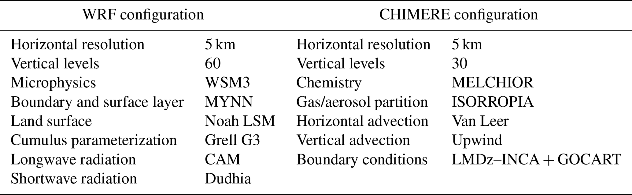
Table A2 Simulation scores for daily average low-level meteorology for wintertime and summertime in 2015. T2 is the 2 m air temperature (in degrees Celsius), RH is the surface relative humidity, U10 is the 10 m zonal wind, and V10 is the 10 m meridional wind speed (m s⁻¹). MB is the mean bias, NRMSE is the normalized root mean square error, and R is the Pearson correlation coefficient.

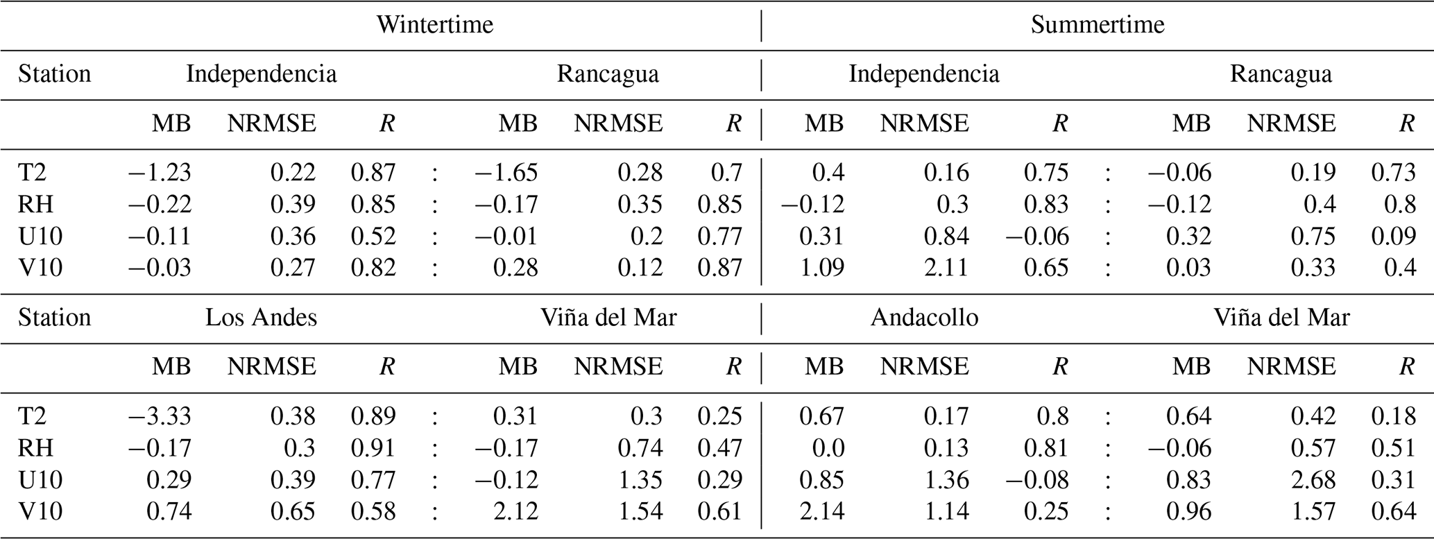
Table A3 Simulation scores for meteorological vertical profiles for 4 d in July 2015 at 12:00 LT at Quinta Normal station in Santiago. T is the air temperature, RH is the relative humidity, U is the zonal wind speed, and V is the meridional wind speed along the vertical profiles.

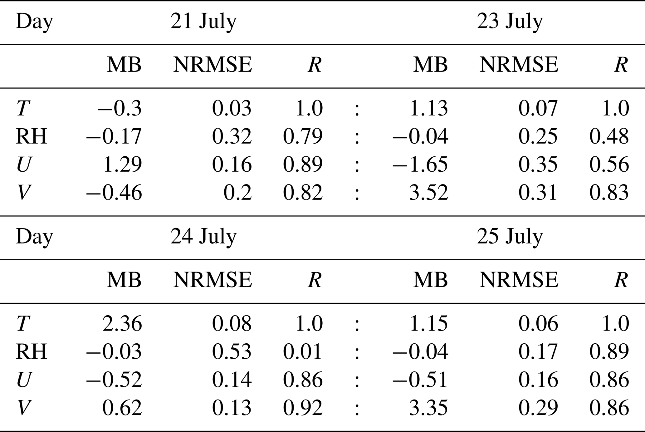
Figure A1 Isoprene (C₅H₈) average emission rate from biogenic sources for 29 January, as computed in CHIMERE using the MEGAN model.

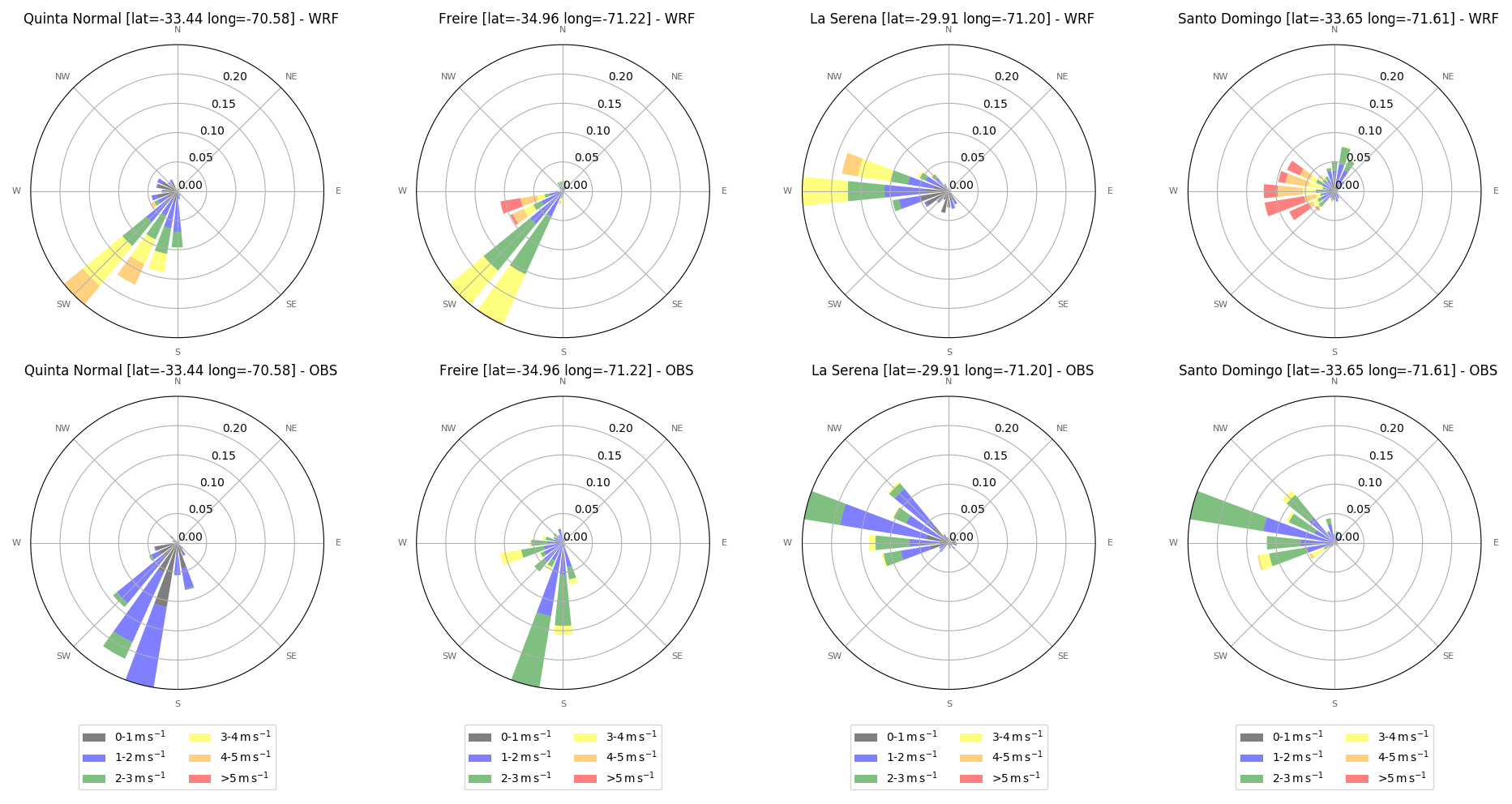
Figure A2 The 10 m wind distribution in the simulation (top) and observations (bottom) at four locations in central Chile for summertime in 2015.

Figure A3 Same as Fig. A2 for wintertime in 2015.

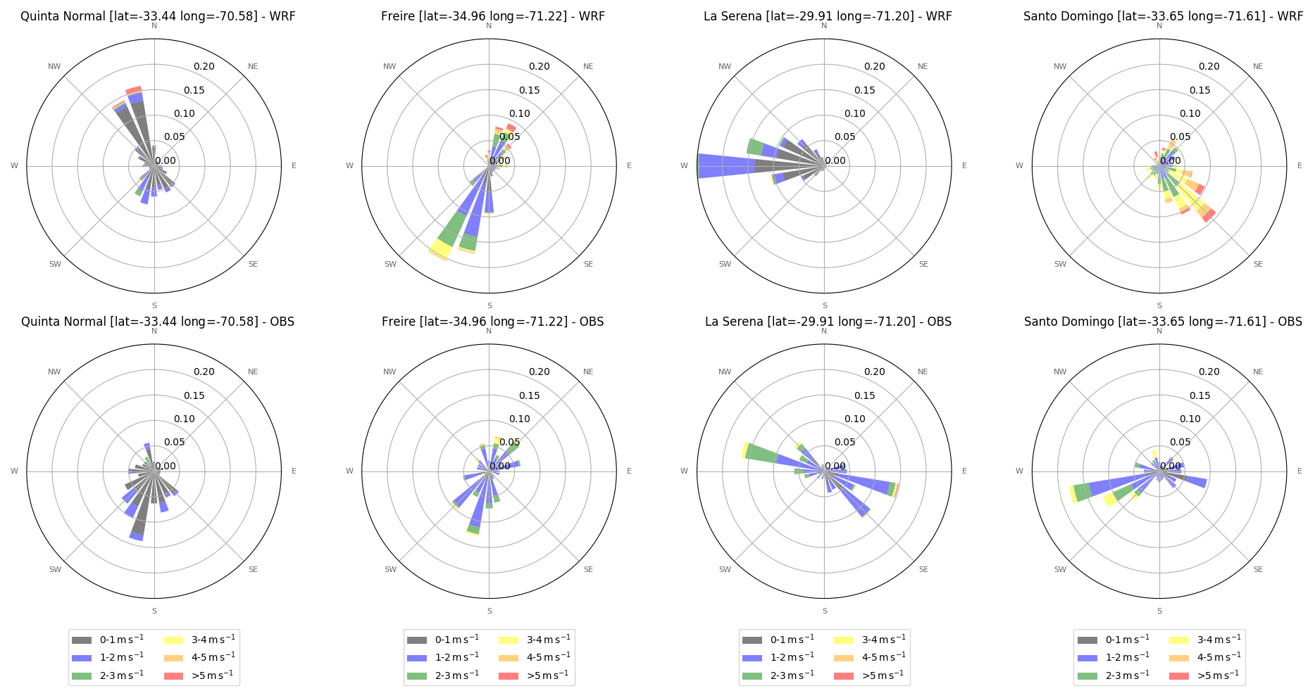
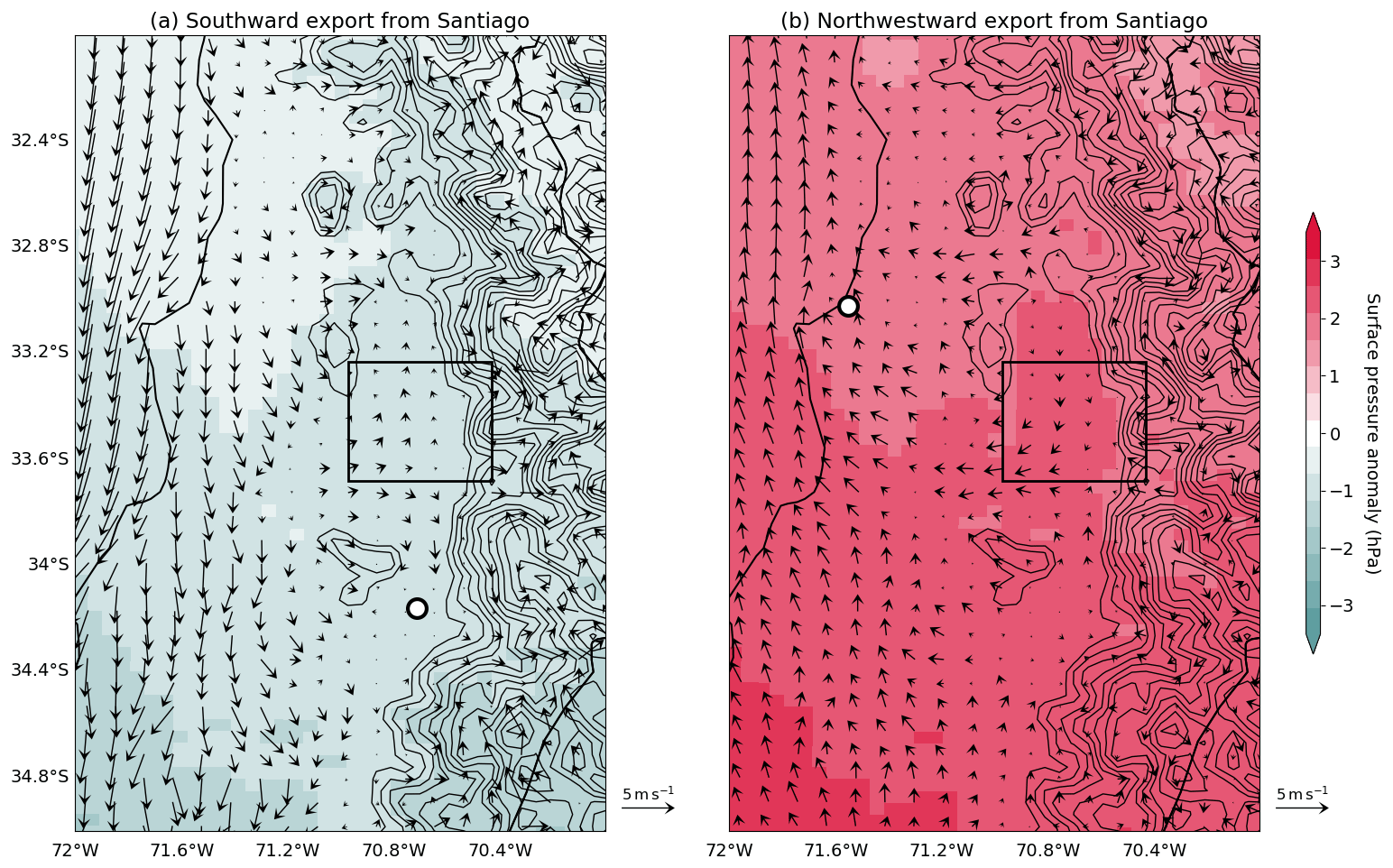
Figure A4 (a) Composite of surface wind (arrows) and pressure (color map) anomalies, with respect to the wintertime average, for hours of southward transport episodes, defined as hours when the concentration of PM_2.5 from Santiago (black rectangle) in Rancagua (white dot) is greater than or equal to its 90th percentile for the period. Contours show terrain elevation in excess of 1000 m every 250 m. Panel (b) is the same as panel (a) but during hours of northwestward transport, defined in the same manner but with respect to concentrations in Viña del Mar (white dot).

Figure A5 (a) Simulated NO_x concentrations (color map), wind (arrows), afternoon boundary layer (white solid line), and terrain elevation (black area) along the summertime transect considered in Fig. 9a, showing the average for summertime in 2015. Panel (b) is the same as panel (a) for NMVOC. Panel (c) is the same as panel (a) for chemical regime. Panel (d) is the same as panel (a) for peroxyacetyl nitrate (PAN).