the Creative Commons Attribution 4.0 License.
the Creative Commons Attribution 4.0 License.
 | 26 Apr 2021
Background conditions for an urban greenhouse gas network in the Washington, DC, and Baltimore metropolitan region
Israel Lopez-Coto
Sharon M. Gourdji
Kimberly Mueller
Subhomoy Ghosh
William Callahan
Michael Stock
Elizabeth DiGangi
Steve Prinzivalli
James Whetstone
As city governments take steps towards establishing emissions reduction targets, the atmospheric research community is increasingly able to assist in tracking emissions reductions. Researchers have established systems for observing atmospheric greenhouse gases in urban areas with the aim of attributing greenhouse gas concentration enhancements (and thus emissions) to the region in question. However, to attribute enhancements to a particular region, one must isolate the component of the observed concentration attributable to fluxes inside the region by removing the background, which is the component due to fluxes outside. In this study, we demonstrate methods to construct several versions of a background for our carbon dioxide and methane observing network in the Washington, DC, and Baltimore, MD, metropolitan region. Some of these versions rely on transport and flux models, while others are based on observations upwind of the domain. First, we evaluate the backgrounds in a synthetic data framework, and then we evaluate against real observations from our urban network. We find that backgrounds based on upwind observations capture the variability better than model-based backgrounds, although care must be taken to avoid bias from biospheric carbon dioxide fluxes near background stations in summer. Model-based backgrounds also perform well when upwind fluxes can be modeled accurately. Our study evaluates different background methods and provides guidance in determining background methodology that can impact the design of urban monitoring networks.
- Article
(2363 KB) - Full-text XML
- BibTeX
- EndNote


In efforts to increase sustainability and address climate change, governments, private entities, and other stakeholders are tracking their greenhouse gas (GHG) emissions over time. Atmospheric observations have a crucial role to play in this effort, as they have the potential to provide a useful tool for assessing the effectiveness of emissions mitigation efforts. Urban atmospheric GHG monitoring networks have proliferated in the past decade, established by the carbon cycle research community to assess the ability of such networks to detect trends and anomalies in urban emissions (Mitchell et al., 2018; Sargent et al., 2018; Lauvaux et al., 2020). Emissions estimates from such atmospheric observations rely on separating observed concentrations into two components: the concentration in the air entering the study domain and the enhancements in concentration attributable to emissions within the domain. This enhancement isolation is necessary for analysis, whether it be for formal statistical inverse modeling of surface fluxes or for unbiased trend detection. In urban areas, background determination is often difficult given the typically smaller study domain and the temporal and spatial variability of the background conditions relative to regional or global studies (Mueller et al., 2018; Balashov et al., 2020; Xueref-Remy et al., 2018).
Previous GHG studies in urban regions have utilized observations from a variety of platforms, including aircraft, ground-based column instruments, satellites, and in situ stationary locations (such as rooftops or towers). Different approaches have been used to isolate the background from observed concentrations from any of these platforms in order to perform analysis on enhancements. Urban analyses based on ground-based in situ GHG observations often establish background concentrations using measurements from stations outside the urban domain, either upwind (often filtering data for a given wind sector) or in an area far from urban emissions. Sometimes these are from observations from a remote or baseline station, such as a mountain top or off-shore location (Mitchell et al., 2018; Verhulst et al., 2017). These background measurements are filtered for clean conditions to remove pollution events for example. A lowest percentile method has also been used as background, e.g., the lowest 5 % of measurements during a certain time period, or a network-wide minimum value (Shusterman et al., 2016; Ammoura et al., 2016). In many studies, observations from a station that is upwind given daily meteorological conditions are used for background (Xueref-Remy et al., 2018; Lauvaux et al., 2016; Breon et al., 2015; Balashov et al., 2020), most often using observations from the same time of day as the urban station. A recent study of carbon dioxide (CO2) in Boston used a more complex back-trajectory-based method to sample the upwind station (Sargent et al., 2018). The background could also be optimized along with the urban fluxes within the inverse analysis (Nickless et al., 2018).
The goal of this study is to construct and evaluate a background for the Northeast Corridor Washington DC/Baltimore tower-based urban network described in Karion et al. (2020). We investigate many of the methods mentioned above, with some exceptions: we do not investigate the baseline/remote station, low-percentile, or optimized background methods. The Washington/Baltimore region is downwind of many large flux regions (both anthropogenic and biospheric), and previous work has shown large synoptic variability in the background for the urban area (Mueller et al., 2018), so the use of a remote station or a lowest percentile method is not likely to produce an accurate representation of background variability. Optimizing the background in an inversion framework along with fluxes could be an option for our domain, but we do not perform an inverse analysis here. Instead, we present some background options that could be used as initial guesses, or priors, in a Bayesian framework for optimization in the future.
Although the analysis we present is focused on CO2 and methane (CH4) in the Washington DC/Baltimore urban domain, we expect many of the overall methods for background estimation and evaluation explored in this study to be extensible to other urban or regional networks. In Sect. 2, we outline the methods for the study, including how we determine background values for the Washington DC/Baltimore network. In Sect. 3, we perform a synthetic data analysis to evaluate CO2 biases in three methods that use upwind observations from surface stations near the domain edge. We use the synthetic experiment to determine the best way to use these upwind observations. In Sect. 4 we evaluate CO2 and CH4 background time series constructed in different ways, including methods that rely on modeled upwind fluxes, against observations and compare their performance. Section 5 includes discussion of the results, and Sect. 6 gives conclusions and recommendations.
2.1 Definition of domain and background
Here we define the background for a given urban measurement as the mole fraction that would be observed at that location and time in the absence of any GHG fluxes inside the domain of interest. Therefore, we separate the CO2 or CH4 mole fraction measured at each station (y) as a combination of a background (yBG) and an enhancement from fluxes within the domain of interest (yenh):
We note that yenh may be positive or negative, depending on the direction of fluxes in the domain. For our study, this domain is an area approximately 140 km by 135 km surrounding the cities of Washington, DC, and Baltimore, MD, and encompassing their larger metropolitan areas (Fig. 1). A network of observation stations on existing towers has been established by Earth Networks and NIST comprising 11 urban towers, i.e., towers situated inside the domain, and 3 background towers, i.e., towers situated near the edges (TMD, SFD, and BUC in Fig. 1). Locations were determined by network design studies (Lopez-Coto et al., 2017; Mueller et al., 2018). Details on the atmospheric CO2 and CH4 mole fraction measurements from this network are found in Karion et al. (2020). In this study we use observations from the six urban sites in Fig. 1, as we focus on November 2016 through October 2017, when only these six had been established. In this work, CO2 measurements are given as dry air mole fractions, with units of µmol mol−1, or parts per million (ppm); CH4 dry air mole fractions are in units of nmol mol−1, or parts per billion (ppb).
2.2 Transport model
Many of the methods we use for estimating yBG rely on a transport model simulation of the domain. We use meteorological fields from the Weather Research and Forecast (WRF) model to drive the Stochastic Time-Inverted Lagrangian Model (STILT; Lin et al., 2003). Following Lopez-Coto et al. (2020a), WRF is configured with the RRTMG radiation scheme (Mlawer et al., 1997), Thompson microphysics scheme (Thompson et al., 2004, 2008), Noah land surface model (Chen and Dudhia, 2001), Kain–Fritsch cumulus scheme (for the 9 km domain only) (Kain, 2004), 1.5-order closure scheme MYNN (Nakanishi and Niino, 2004, 2006) with the eddy mass-flux option (Olson et al., 2019) and the land-use classification from the 2011 National Land Cover Database (Homer et al., 2015). Three nested domains are used (9, 3 and 1 km), with the innermost domain covering the urban area of interest, with 60 vertical levels with monotonically increasing thickness from the surface (34 levels below 3 km) and driven by initial and boundary conditions from the North American Regional Reanalysis (NARR) 3-hourly data (Mesinger et al., 2006).
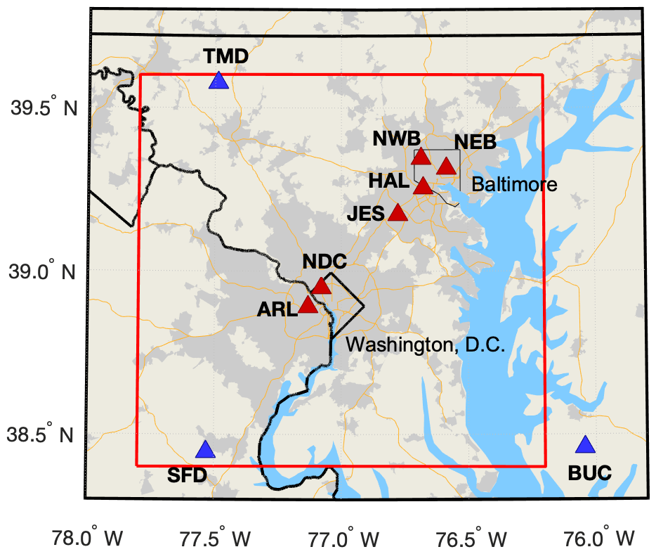
Figure 1Domain of interest for our study (red square), surrounding the metropolitan regions of Washington, DC, and Baltimore, MD. Gray shading indicates U.S. Census-designated urban areas (http://www.census.gov, last access: 23 March 2017). Red triangles indicate urban stations used in this study, and blue triangles indicate background stations. All map data layers obtained from either Natural Earth (naturalearthdata.com) or U.S. Government sources and in the public domain.
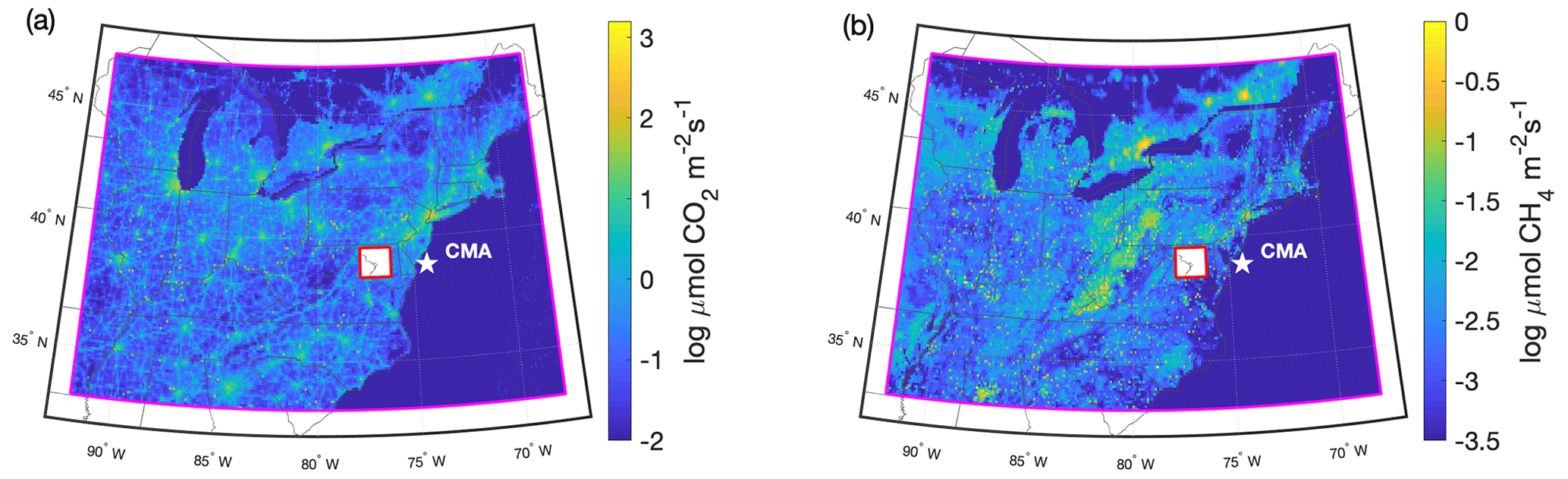
Figure 2Maps of nested domains used to calculate the two-component background. The outer domain (magenta) is used to determine the near-field background (yBGnear) using footprints from STILT and existing flux inventories. (a) January 2015 mean of fossil-fuel CO2 from Vulcan 3.0 with FFDAS in the Canada portion of the domain is shown in log scale. (b) January 2015 mean of the EPA CH4 inventory with EDGAR in the Canada portion of the domain is shown in log scale. A global model is sampled at the edge of the outer domain for the far-field background (yBGfar). The red square over Washington, DC, and Baltimore, MD, corresponds to the domain shown in Fig. 1. The white star indicates the location of the NOAA aircraft site CMA. All map data layers obtained from U.S. Government sources and in the public domain.
STILT generates influence functions, or footprints, that relate the enhancement measured at a given observation location to fluxes from an area at the surface. STILT also tracks mass-less particles backward in time, and here we use the particles from each observation to determine the location and time of exit from the domain (i.e., this is analogous to the location of entry of each air parcel into the domain before eventually reaching the observation point). For this work, we emit 960 particles for each hourly mean observation from both urban and background towers. Particles are released over the entire hour to simulate the hourly mean and tracked back in time for 5 d. Footprints are calculated for two nested domains: an inner domain with a footprint gridded at 0.01∘ (shown in Fig. 1) and an outer domain with a footprint gridded at 0.1∘ (Fig. 2); the exit points of the particles are determined for both domains. The choice of the two domains was made specifically for our region in order to capture large emissions sources and other urban areas outside Washington, DC, and Baltimore. The simulation time for STILT of 5 d was chosen so that most of the particles (over 90 %) had exited the larger of the two domains by that time. The analysis covers the 1-year time period from November 2016 through October 2017.
2.3 Sampling a global model at the urban domain boundary
In the next few sub-sections we describe several methods for estimating the background that we investigate in this work (Table 1), beginning with methods relying on global model output.
Table 1Summary of background methods compared and evaluated for CO2 and CH4. References for all the models can be found in the pertinent Methods section.
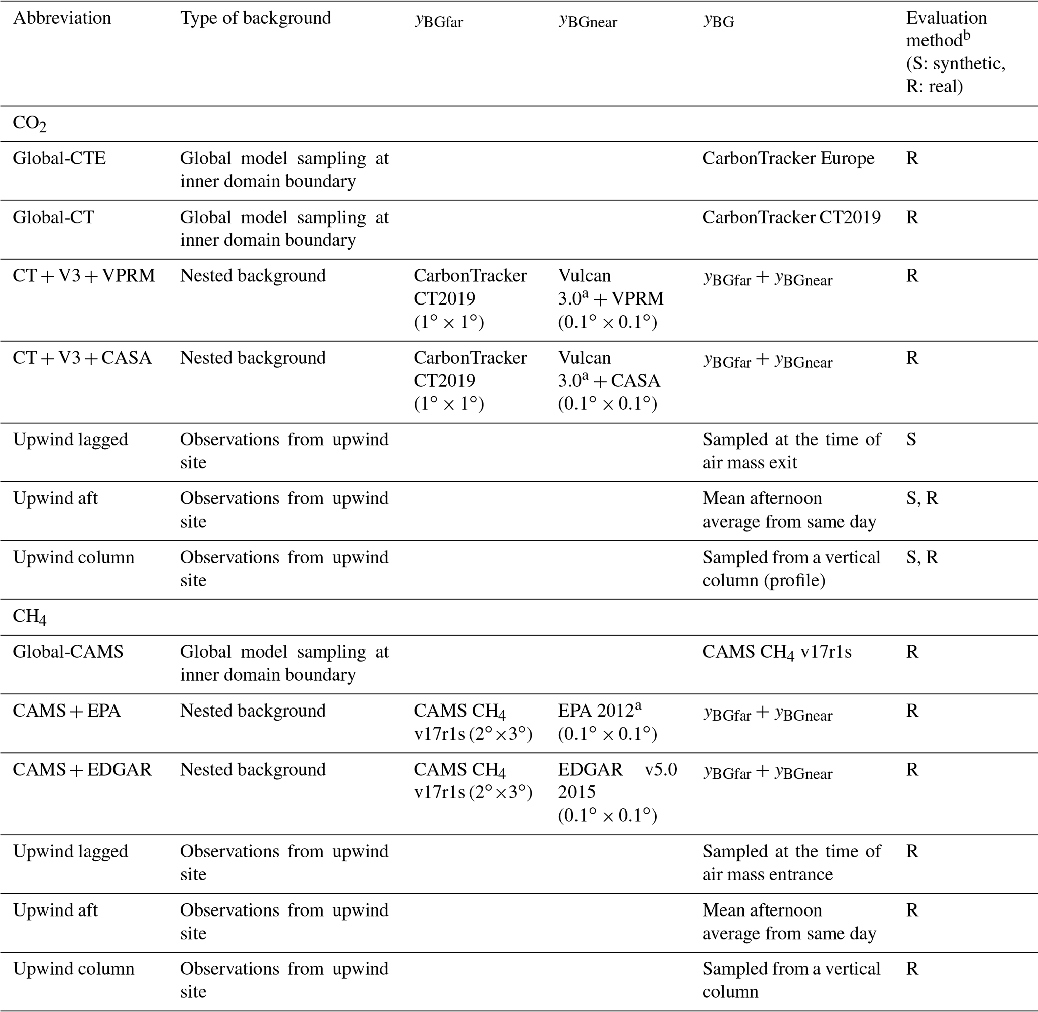
a Models using Vulcan 3.0 as the flux in the near-field background use FFDAS 2015 and models using EPA use EDGAR v4.2 for the small region in Canada within our outer domain (Fig. 2). b The rightmost column indicates whether this background was evaluated in the synthetic data study (S; Sect. 3) or against actual (real) observations (R; Sect. 4).
In the global model method, a 4D field of the GHG mole fractions from an existing global model is sampled by each STILT particle as it exits (enters) the urban domain (Fig. 1) at a given latitude, longitude, altitude, and time. Here, for CO2 we use publicly available mole fraction output from two different global CO2 inversion models: CarbonTracker (CT) version CT2019 (http://carbontracker.noaa.gov, last access: 6 January 2020; Peters et al., 2007; Jacobson et al., 2020) and Carbon Tracker Europe (CTE (obtained by request); Peters et al., 2010). These two are referred to as Global-CT and Global-CTE (Table 1). Both global models provide vertically resolved, 3-hourly, 1∘ resolution CO2 mole fraction fields. For CH4, we use the Copernicus Atmosphere Monitoring Service (CAMS) global inversion 4D fields at 4-hourly, ∘ resolution (v17rs1, available at https://apps.ecmwf.int/datasets/data/cams-ghg-inversions/, last access: 26 April 2019; Segers and Houweling, 2018) (Global-CAMS). The advantage of sampling a global model as a background is that the mole fraction field varies in space and time, and this field is generated from fluxes optimized using atmospheric observations. A disadvantage, however, is the global models' resolution is quite coarse relative to our small (∼140 km across) domain and may not provide sufficient spatial resolution for the background (i.e., the entire domain is only slightly larger than one CarbonTracker grid cell).
2.4 Using a nested domain to define a two-component background
A second method of estimating a background is to use a nested domain and separate the background yBG from Eq. (1) into two components (Eq. 2).
The first component, yBGfar, is obtained by sampling a global model as described above but at a boundary far from the domain of interest (magenta boundary in Fig. 2). The second component, yBGnear, is determined from convolutions of STILT footprints with a flux field in the outer domain. The fluxes within the inner domain of interest are set to zero, so that yBGnear does not include any enhancements from the inner domain. It only represents enhancements from fluxes between the outer domain and the inner domain (Fig. 2 shows examples of these fluxes).
One disadvantage of this two-component background is that, in our case, the fluxes used in the outer domain are not optimized using atmospheric observations; we rely on existing inventories and biospheric models. In addition, the existing anthropogenic inventories were developed for a different year than the study (for both CO2 and CH4), introducing additional uncertainty. However, the spatial resolution of the fluxes and meteorological model is better than for the global models (9 km for WRF and 0.1∘ for the fluxes vs. 1∘ or more for the global models) and thus may better capture variability in background concentrations. We also can use different flux fields to estimate a range of background options using this method. For CO2 we have used Vulcan 3.0 (Gurney et al., 2020b, a) for anthropogenic fluxes in the US and the Fossil Fuel Data Assimilation System (FFDAS) (Asefi-Najafabady et al., 2014) in Canada. Both products are for the year 2015 and are adjusted to match the day of the week in the study year (2016/17) (Fig. 2a). We also use output from two biosphere models: a custom Vegetation Photosynthesis and Respiration Model (VPRM) (Gourdji et al., 2021) and an ensemble mean of the Carnegie-Ames-Stanford Approach (CASA) model run (Zhou et al., 2020) for biosphere fluxes (both for the time period of our study). We refer to these two combinations as CT + V3 + VPRM and CT + V3 + CASA (Table 1). For CH4, we have used the EPA 2012 gridded inventory (Maasakkers et al., 2016) (Fig. 2b) and EDGAR v5.0 2015 (https://edgar.jrc.ec.europa.eu, last access: 11 February 2020; Crippa et al., 2019) (referred to as CAMS + EPA and CAMS + EDGAR, respectively). We do not expect large biases in the anthropogenic CO2 inventory fluxes at this regional scale, but the CH4 and biosphere CO2 fluxes are less well-known and may introduce error. Specifically, this method is problematic for CH4, where existing inventories have been shown to disagree significantly with measurements in the region upwind of our domain, likely due to underestimation of oil and gas emissions (Barkley et al., 2019). We also note that these inventories are for different years than our study. One future goal of our project is to use inverse modeling to optimize fluxes in the outer domain to improve the accuracy of the background for the inner domain.
2.5 Using observations upwind of the urban domain, three different ways
Observations upwind of the domain of interest have been the most commonly used choice for background for urban studies (Lauvaux et al., 2016; Sargent et al., 2018; Nickless et al., 2018). The advantage to using observations over model-based estimates is clear: there is no need to depend on a global model or assume upwind fluxes are known. A background station also captures the variability in time that is expected of the background but will not capture the variability in space, a consideration in this area with large spatial variability in upwind fluxes. In this study, we determine the upwind station as the location that minimizes the difference between the mean particle exit angle and the angle to the background site. First, each particle from our WRF-STILT model of an urban tower observation is tracked back to its exit location from the domain, and the nearest background station is determined by comparing the exit angle and the angle between the background site and the urban station. We choose between the stations in Thurmont, MD (TMD), Stafford, VA (SFD), and Bucktown, MD (BUC). If the nearest station does not have observations for the time that the particle exited, the next nearest is used. Until May 2017, only one background site was operational, BUC, meaning that backgrounds constructed using any of the upwind-observation-based methods always use BUC until May 2017, when TMD was established. SFD was established in July 2017, so after that period all three stations were options. Note that in the synthetic data study, we use all three sites for the entire year as the ideal case scenario and then investigate the effect of using only one site without filtering for particular wind directions, as other studies have done.
In this section, we describe three ways to use measurements from an upwind measurement station and then evaluate them for CO2 in Sect. 3 using a synthetic data study. We choose the best method among these to evaluate along with model-based methods for both CO2 and CH4 in the real data study (Sect. 4).
2.5.1 Upwind lagged method
We investigate using measurements from an upwind station in a truly Lagrangian fashion, i.e., to sample the upwind observations at the time an air parcel enters the domain of interest. This is typically not an effective method because at earlier times of the day, the mixing depth is often shallower than it is later in the day, and this method does not account for dilution of concentrations due to a growing planetary boundary layer (PBL). The background will be biased high and, thus, the enhancement determined at the urban tower would be negatively biased. In a synthetic data investigation of how to site background stations, Mueller et al. (2018) showed that although the upwind measurements sampled in this manner correlated well with the true background at the urban sites, they were biased high.
2.5.2 Upwind afternoon method
A common method for overcoming the problem of diurnally varying boundary layer depth is to approximate the dilution in concentration by using upwind observations at the same time as the observations at the urban site, when the PBL is similar between the two (e.g., Lauvaux et al., 2016). In our case, because we restrict our analysis to afternoon hours at the urban sites, this translates to sampling the upwind tower in the afternoon as well. This method must be considered carefully, and its effectiveness depends on the specific geography and location of the urban and rural measurement stations as well as the size of the domain. For example, on a summer day, a rural upwind tower at mid-day could be influenced by strong local photosynthetic uptake causing a bias relative to the air measured at the urban tower at the same time; even if the same air mass passed the upwind tower, it did so earlier in the day when there was less uptake. Another concern is that on days with more complex or shifting winds, the upwind tower may not represent air originating in the same area as the air mass sampled farther downwind in the city. In a smaller domain, transit times to the boundaries are shorter in general, and this effect may not cause much error. Otherwise, to alleviate the effect of these near-field fluxes when using a background observation at the same time as the urban observation, modeled enhancements (estimated using inventories inside the domain) from sources within the domain could be subtracted from the upwind concentration (Lauvaux et al., 2016). However, if near-field fluxes outside the model domain influence the upwind towers (as is the case in our domain, because our background towers are either very close to the edge or outside the domain entirely), this correction may not entirely eliminate the problem.
2.5.3 Upwind column method
This method accounts for dilution by free tropospheric air being entrained into the growing PBL by sampling the upwind location using an ensemble of particle trajectories from STILT, as was done to sample the global model (Sect. 2.3). This method has been used previously in regional studies to sample an upwind curtain that was constructed using smoothed long-term measurements (Jeong et al., 2016; Karion et al., 2016). In those studies, the STILT particles were used to sample a mole fraction field (curtain) at the edge of the domain with latitudinal, vertical, and temporal variability. Unfortunately, in our case, we do not have enough upwind measurements to construct a full boundary curtain. Instead, we combine the idea of sampling a background curtain using the particles' exit locations and times with the idea of sampling an upwind measurement station, similarly to Sargent et al. (2018). We construct vertical profile columns of CO2 and CH4 that do not vary laterally but allow the particles to sample a realistic vertical mole fraction gradient and average the mole fractions in the column across the particles to calculate at the background value (yBG). Below we describe the method for constructing vertical profile CO2 and CH4 columns at upwind sites for use with this method.
For every urban observation that we model using STILT, we construct a vertical profile, or column, background to sample with the particle trajectories. Once the background station is identified using the particle trajectories as described earlier, the modeled boundary layer height associated with the exiting particle's exit location and time is used to construct a vertical profile y(z) as shown in Eqs. (3) and (4) and described below, where y is the mole fraction in the column and z is the altitude above ground level (a.g.l.). We define two cases: one for afternoon hours (Eqs. 3a and 3b) and one for non-afternoon hours (Eqs. 3c through 3e); note that the time of day referred to here is the local time at which the particles exit the domain, not the time of the urban observation.
Afternoon hours:
Non-afternoon hours:
where the parameters A and B are constants calculated by imposing two boundary conditions on Eq. (3d):
If the particle exited during afternoon hours (defined as 5 h after sunrise and before sundown), then the profile represents a two-layer troposphere consisting of the background site observation (yobs) from the ground to the top of the PBL and the free troposphere value, yFT (discussed below), above the PBL (Eqs. 3a and 3b). If the particle exits during non-afternoon hours, the profile is constructed in three layers. The lowest layer, below the PBL, consists of the observation at the background tower at the exit time, yobs (Eq. 3c). From the PBL to 2000 , the profile is assumed to be a residual layer and is modeled as an exponential decay function beginning with the tower observation (yobs) at the PBL top to the concentration measured at that same site the previous day (mid-day afternoon average), yprevAFT (Eq. 3d). Above 2000 , the profile is based on the free-tropospheric value yFT (Eq. 3e). The height of the residual layer (2000 m) and the length scale of the exponential function (800 m) were determined using the synthetic experiment described in Sect. 3 by testing several values and choosing the best-performing combination (not shown). The choices for both of these values introduce error in the column background; for example, the height of the residual layer would change from day to day, and here it is assumed constant.
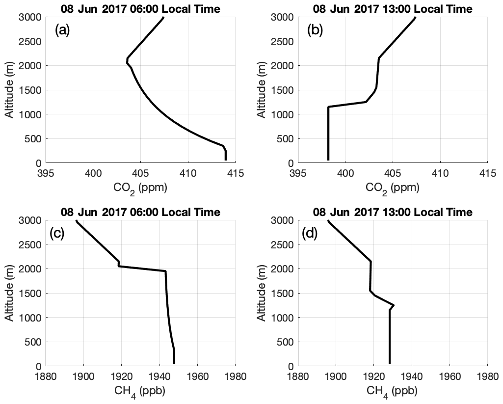
Figure 3Examples of CO2 (a, b) and CH4 (c, d) vertical column profiles above BUC for morning (a, c) and afternoon (b, d) on a summer day with winds from the east (i.e., when the site is upwind of the urban domain). Profiles are constructed as described in the text.
The free-tropospheric mole fractions for all profiles (yFT) are derived from binned and smoothed CO2 and CH4 observations from the National Oceanic and Atmospheric Administration's Global Monitoring Laboratory (NOAA/GML) regular aircraft sampling at site CMA (Sweeney et al., 2015), available from the CO2 GLOBALVIEWplus v5.0 ObsPack (Cooperative Global Atmospheric Data Integration Project, 2019) and the CH4 GLOBALVIEWplus v2.0 ObsPack (Cooperative Global Atmospheric Data Integration Project, 2020). These observations are made on flights conducted approximately every 2 weeks collecting whole-air samples in flasks at nine altitudes between 300 and 8000 , offshore and almost directly east of our domain (Fig. 2). We assume that the CMA observations above 2000 m are not influenced by fluxes in our inner domain and are representative of typical seasonally varying concentrations in the free troposphere above our domain. We bin the data into nine altitude bins between 0 and 9000 m designed to evenly distribute observations between bins and use the ccgcrv software from NOAA/ESRL (Thoning et al., 1989), available and documented at https://www.esrl.noaa.gov/gmd/ccgg/mbl/crvfit/crvfit.html (last access: 15 June 2018), to smooth the time series within each altitude bin with four annual harmonics and three polynomial terms. Example profiles over BUC are shown in Fig. 3.
To evaluate the three upwind-observation-based CO2 background conditions described in Sect. 2.5, a synthetic data experiment was devised similar to that described in Mueller et al. (2018). CO2 was chosen rather than CH4 because we believe we have a relatively realistic flux field to use for CO2, whereas for CH4, we find large differences between model estimates and observations. In particular, BUC is in an area with a large influence of local wetlands (Karion et al., 2020), so that the synthetic experiment would not yield necessarily realistic results without an accurate wetland model. The same-day afternoon sampling of CO2 is also more likely to be a problem due to strong biospheric fluxes in summer influencing observed concentrations at the background station; whether the column method alleviates this issue was a key question to answer with the synthetic experiment.
A set of synthetic CO2 observations y was constructed using the WRF-STILT footprints from our model for 5 November 2016 through 30 October 2017, for six urban sites (NWB, NEB, HAL, JES, NDC, and ARL) and all three background sites (BUC, SFD, TMD) for the entire time period; see Fig. 1 for locations). Note that in order to evaluate the effectiveness of the method, we simulated all three upwind sites for the entire year even though in reality two of them were established later in the year (May 2017 and July 2017 for TMD and SFD, respectively). The nested domain setup was used to construct observations for each afternoon hour at the urban sites (afternoon defined as the period between 5 h after sunrise until sundown):
For the synthetic observations, yBGfar is derived by sampling CarbonTracker CT2019 at the edge of the outer domain (Fig. 2). yBGnear is derived from convolving WRF-STILT footprints in the outer domain with 2015 Vulcan 3.0 (Gurney et al., 2020b) (with FFDAS for the small Canadian portion of the domain) anthropogenic fluxes and VPRM (Gourdji et al., 2021) with zero fluxes in the inner domain. In other words, we construct the “true” background as CT + V3 + VPRM as defined in Table 1. Although the anthropogenic flux data products are derived for the year 2015, they represent a plausible representation of sources in our domain for this synthetic experiment. The enhancement from fluxes in the inner domain, yenh, is the convolution of the footprints in the inner domain with Vulcan 3.0 and VPRM. Thus the true background, , is known for each synthetic observation y.
We also construct observations y for all 24 h at the background sites (BUC, TMD, SFD) in exactly the same manner and use them to construct the synthetic upwind column background described in Sect. 2.5.3. For the synthetic column, free-troposphere values are sampled from CarbonTracker CT2019 (Jacobson et al., 2020) at the CMA location. Thus, the experiment assumes perfectly known transport and perfectly consistent fluxes and allows for the determination of how well a column background sampled above an upwind site represents the true background observed by the urban towers at any given afternoon hour. We also determine a background based on sampling the synthetic observations at the upwind site at the same time as the urban site (i.e., upwind afternoon observations, as described in Sect. 2.5.2, with modeled in-domain enhancements removed) and sampling the upwind site at a lagged time based on particle exit (i.e., upwind lagged observations, Sect. 2.5.1) to quantify the biases in these three methods.
We evaluate the error (defined as the true background subtracted from the background constructed using upwind observations) by looking at the mean as a function of different factors: month of the year (Fig. 4a), mean distance from the background site (Fig. 4b), mean trajectory exit altitude (Fig. 4c), and mean trajectory exit time of day (Fig. 4d). The overall annual statistics (mean bias, standard deviation, and R2) (Fig. 4a) indicate that the column-based background (red) is the best performer. The results also indicate that sampling the upwind site at the time the air mass entered the domain (upwind lagged) yields a high bias in the background (as described in Sect. 2.5.2) due to PBL dynamics (blue). Using the upwind observations from the mid-afternoon (upwind aft) causes a summertime negative bias due to biospheric uptake (negative fluxes) near the upwind tower (green). Figure 4d indicates that the largest errors in the non-column backgrounds occur when the air mass enters the domain early in the morning, as is typical when using afternoon observations in this domain.
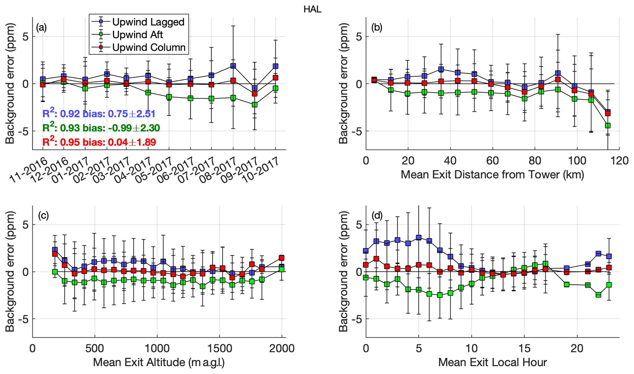
Figure 4Results of the synthetic data study. Error in background (constructed background–true background) at HAL (afternoon hours only) for each method of using upwind site observations described in the text. Results for the other urban towers are similar. Red points indicate the column-based background (upwind column); green from sampling upwind sites at the same time as urban sites (upwind aft); blue from sampling upwind sites at the time of the particle exit (air mass entrance) earlier in the day (upwind lagged). Text in (a) indicates the coefficient of determination (R2) and mean bias ± 1 standard deviation of the error over the entire year for each method in the corresponding colors. (a) Monthly mean, (b) binned by mean particle exit distance from the closest upwind tower, (c) binned by mean exit altitude, and (d) binned by mean exit time of day. Error bars are standard deviations.
These results support using the upwind site observations at the same time as the downwind observations (upwind aft) if diurnally varying fluxes near the upwind tower are not a concern (for example, for fossil-fuel CO2 only or wintertime only) or for instances where the domain is small enough that the transit time is short between the two stations. Otherwise, strong biosphere fluxes near the background sites that are unaccounted for can cause an overall summertime bias in the background at monthly scales. This conclusion may not be extensible to other network configurations (for example, depending on the location of background sites in relation to strong biological fluxes) but shows that for the network design here, sampling the background site at the same time as the urban site gives a biased background in summer. Figure 4c indicates that the biases in non-column methods occur when particles exit at higher altitudes, likely because these methods do not account for mixing of air from the free troposphere into the urban domain. However, they also show that the column-based background, as constructed here, does well at eliminating these biases. Figure 4 shows the results for one site (HAL) only, but the results do not vary much between sites (annual biases range from −0.02 to 0.16 ppm; root-mean-square error (RMSE) ranges from 1.81 to 1.91 ppm).

Figure 5Results from synthetic experiment. (a) Fraction of STILT particle trajectories exiting closest to each background tower by month (MM-YYYY). (b) Bias and (c) RMSE for column-based upwind backgrounds (relative to the true background) in the synthetic data experiment using only a single background site (shades of blue), compared with the ideal scenario of all three background towers having available observations (red). Average values over the six urban sites for each month are shown.
As noted earlier, synthetic observations from all three background towers were used in this analysis, even though SFD and TMD were not established for some of the time period. Somewhat surprisingly, we do not see a large bias as a function of the distance between the exit trajectory and the upwind station below 100 km (Fig. 4b) but a sharp increase in bias after that. Given that the distance between the trajectory exit and the designated upwind site should affect the error, we also investigated the bias and RMSE for configurations in which only a single background site was available (Fig. 5). Particle trajectory statistics from STILT indicate that most air masses enter the domain closest to TMD, the site in the northwest of the domain, with the fewest entering near BUC for most months of the year (Fig. 5a), confirming that the predominant wind direction for this region is west or northwest. Both monthly biases and RMSE are generally larger when only using a single background site (Fig. 5b and c); as one might expect, biases tend to be positive because the single site may be downwind of the urban area for some time periods, depending on wind directions (e.g., BUC would be downwind when winds are from the west, so observations there would be likely to be enhanced relative to the true background). The RMSE might be further reduced if additional background towers were available; for our domain, specifically, we plan to establish an additional background site in the northeastern corner of the domain. This site should better represent the background when winds are from that direction (14 % of the time), given the likelihood of elevated concentrations entering the domain from upwind urban areas (e.g., Wilmington, DE, or Philadelphia, PA), which are not captured by the current background stations.
The synthetic study described above is valuable in determining how to best use the upwind site observations to construct an unbiased background. From that analysis, we conclude that the upwind column method performs best among the upwind observation methods. However, there are several sources of error that are not accounted for in that setup. Specifically, errors in transport (for example in the modeled PBL depth) would cause errors in the upwind column background, as would errors stemming from the sparse sampling at CMA (which was binned and smoothed), which affect the free tropospheric value used in the upwind column, while in the synthetic study those were modeled using CarbonTracker fields that are fully simulated in space and time. Here we evaluate the upwind column method against the model-based methods described in Sect. 2 and Table 1 against real observations of CO2 and CH4 from the urban sites. Because it is commonly used in urban studies, we also evaluate the upwind afternoon method for comparison, even though we found it to be biased for CO2 in the summer in the synthetic study.
In this real-data comparison, we only use observations during times when we expect minimal contribution to the urban enhancements from the urban domain. The goal is to isolate errors that are most likely to be caused by background choice rather than the flux model inside the domain. To do this, we choose afternoon hours for which the magnitudes of the STILT influence functions (footprints) are in the 10th percentile of all afternoon hours over the entire year-long study period, resulting in 50 to 300 compared observations per month, with generally greater numbers in the summer months due to the longer afternoon time period.
We calculate backgrounds for each urban site observation meeting the footprint strength criteria using multiple methods described in Sect. 2 and summarized in Table 1, all utilizing the same WRF-STILT transport. We chose these as a set of reasonable backgrounds; we also evaluated additional combinations for the nested methods, but there was no significant difference from those shown (e.g., choosing a different product for anthropogenic emissions for yBGnear or a different global model for yBGfar). All combinations use the same fluxes inside the inner domain to calculate yenh: Vulcan 3.0 and VPRM for CO2 and EPA (Maasakkers et al., 2016) for CH4. Modeled inner domain enhancements for these observations range from 0 to 7 ppm of CO2 (2 to 16 ppb CH4) in any given month, with all months except November and January at or below 2 ppm (CO2) and 6 ppb (CH4). Error in the assumed fluxes inside the domain would affect these modeled enhancements and contribute to the errors calculated in this analysis.

Figure 6Average monthly bias (model–observation) (a, c) and RMSE (b, d) for different backgrounds over all six urban sites during periods of low influence from within the domain of interest. (a, b) are for CO2; (c, d) are for CH4. All models use the same fluxes inside the urban domain; only the background varies, as indicated in the legends above each set of panels, with abbreviations from Table 1.
The model bias (modeled–observed) indicates that the upwind column background (red) performs well for CO2 but is negatively biased in the summer months (Fig. 6a). Some positive bias in the upwind background is expected due to the lack of upwind observations available from November through April from TMD or SFD. The synthetic data study had indicated that using BUC alone leads to a high bias because it is not always upwind of the urban area (Fig. 5), but in this evaluation, only January has a positive bias using the upwind column background. There may be an offsetting negative bias; this and some of the negative summertime bias may be caused by inaccuracy in the fluxes inside the domain (Vulcan 3.0 + VPRM) rather than the backgrounds. This result suggests the possibility that the biosphere model is biased in the same direction (too much summertime uptake or too little respiration) or that the error is not from the biosphere model. The anthropogenic emissions in the domain could also be incorrect, affecting this result and possibly offsetting a wintertime positive bias in the background. The upwind aft background (green, Fig. 6a) has an even larger negative bias in summer, a result consistent with the synthetic data analysis. The RMSE indicates significant hourly variability (RMSE ranging from 1 to 8 ppm) in the background errors even when there is little bias (Fig. 6b).
Methane results indicate that the four backgrounds relying on inventory or modeled emissions outside the domain have a negative bias, while backgrounds based on upwind observations (both upwind column and upwind aft) are less biased throughout the year (Fig. 6c). RMSE analysis confirms that the upwind observation-based backgrounds perform better than the model-based backgrounds for CH4. Monthly variability of CH4 RMSE follows similar patterns to CO2 (Fig. 6b vs. d); for example, in April 2017 both show large RMSE values, indicating that some of the error is likely from transport. Figure 6 shows statistics averaged over the six urban sites; monthly patterns in both bias and RMSE for each site are very similar to the mean.
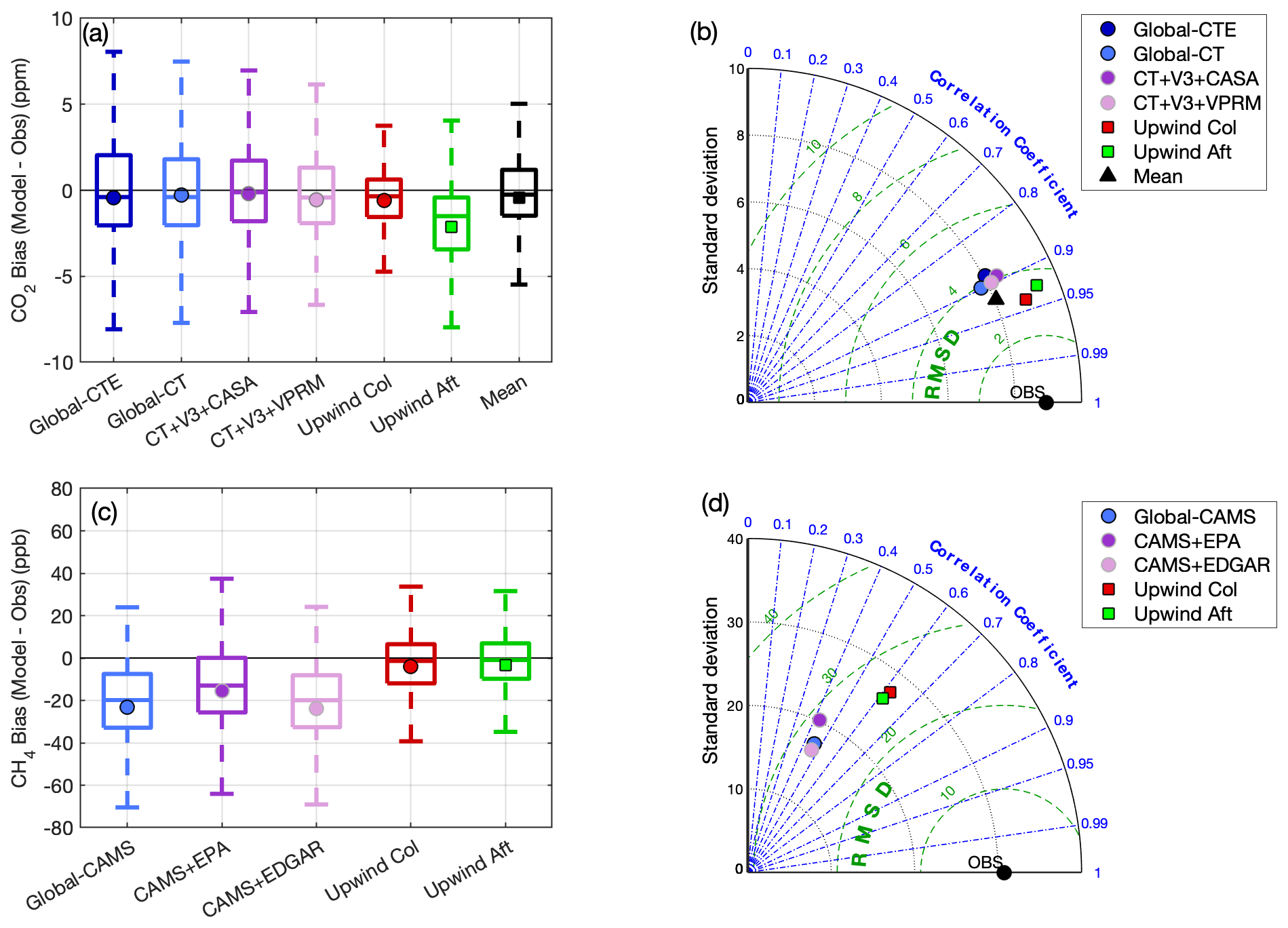
Figure 7Annual statistics for modeled vs. observed mole fractions over all six urban sites for CO2 (a, b) and CH4 (c, d) using identical fluxes in the inner domain with the different backgrounds from Table 1. For CO2, we also include the mean of the first five (excluding upwind aft). (a, c) Bias (model–observations, afternoon hours); center line is the median value of the bias over all low-footprint hours of the year; symbol is the mean; box edges indicate 25th and 75th percentiles (inter-quartile range); whiskers show range excluding outliers; outliers not shown. (b, d) Taylor diagram (Taylor, 2001) illustrating performance replicating the standard deviation of the afternoon observations (black axes at constant radius), correlation (blue angular axes), and root-mean-square deviation (RMSD, green arcs).
Analyzing the full year from all six urban sites together (all afternoon hours, Fig. 7), for CO2, the model-based backgrounds and the upwind column have close to zero net bias over the whole year, but the upwind column background performs best in terms of hourly scatter, as indicated by the smaller inter-quartile range in the box plot (Fig. 7a). The CO2 Taylor diagram (Taylor, 2001) in Fig. 7b indicates that the correlation coefficient is quite high, close to 0.9 for all backgrounds, because they all successfully diagnose the seasonal cycle. The two backgrounds based on upwind observations perform best in terms of correlation coefficient and have lower root-mean-square deviations and standard deviations closer to those of the observations (black circle on the x axis), with the column background (red) performing best. We also evaluate the performance of a background that is the hourly mean of the first five backgrounds, i.e., excluding the upwind aft background which has a distinct low bias. This mean background performs fairly well, although not as well as the upwind column.
We evaluate five similarly constructed backgrounds for CH4 (see Table 1 for specifics), and, just as in the monthly analysis (Fig. 6c and d), find that the two backgrounds based on upwind observations perform best (Fig. 7c and d). Unlike for CO2, using the upwind afternoon observations (green) performs just as well as (even slightly better than, in terms of bias) the upwind column (red), with near-zero bias through the year. Both the bias box plots and Taylor diagram indicate that using an upwind observation for CH4 is highly preferable to a background that relies on modeled emissions, because the models used here (EPA gridded inventory; Maasakkers et al., 2016, and EDGAR v5.0; Crippa et al., 2019, along with the global CAMS inversion; Segers and Houweling, 2018) are likely too low in their outer domain emissions. Correlation coefficients for CH4 are significantly lower overall than for CO2, even for the observation-based backgrounds, due to the lack of a strong seasonal cycle. Interestingly, the correlations are higher for the upwind backgrounds (coefficients close to 0.6) than for the model-based backgrounds (coefficients of 0.4 to 0.5), even though the model-based backgrounds might be assumed to better capture the spatial variability of incoming air, which does not seem to be the case, likely because the poor quality of the emissions products used here negates this advantage. We also note that in the EPA or EDGAR emissions do not include emissions from wetlands, which may explain some of the poor performance especially when winds are from the east. The small negative biases of the upwind aft and upwind col backgrounds over the year (3 and 4 ppb, respectively) are to be expected if emissions inside the domain are lower than the EPA 2012 inventory, which previous work suggests is the case (Lopez-Coto et al., 2020b).
The large hourly variability of error in the background (as indicated in the inter-quartile differences shown in Fig. 7) leads to the question of what the uncertainty is on enhancements from the urban network. This uncertainty is crucial to understanding the signal-to-noise ratio and is often required for any analysis, such as an atmospheric inversion. Unfortunately, the true uncertainty of the background is unknown. However, we can observe the differences between the various realistic and plausible representations of the true background that we have constructed for CO2. We limit this set of plausible backgrounds to the first five backgrounds listed in Table 1 (i.e., omitting the upwind aft background, which we found to be biased in summer). Although this set of five background time series does not represent a formal probabilistic ensemble, the spread of these members can still inform us as to the confidence we have in any one of them or their mean. Here for CO2 we investigate and compare two different proxies for background uncertainty. The first is to use the standard deviation of the first five backgrounds listed in Table 1. The second is to use the standard deviation of the difference between modeled and observed CO2 when using the best-performing background (in our case, upwind column as shown in Sect. 4) during times of low domain influence (i.e., the data shown in the box plot in Fig. 7a). These two quantities (shown as monthly means in Fig. 8) have similar magnitudes in winter months, but the uncertainty estimated using the modeled-to-observation difference during low footprints (red) is larger in the summer. As this second method also includes uncertainty from the fluxes inside the domain, it may be an overestimate of the uncertainty. Note that we cannot estimate the uncertainty for CH4 using the set of backgrounds in Table 1 as the four model-based backgrounds are clearly underperforming relative to the other two, so they cannot be considered realistic or plausible representations of the true background.
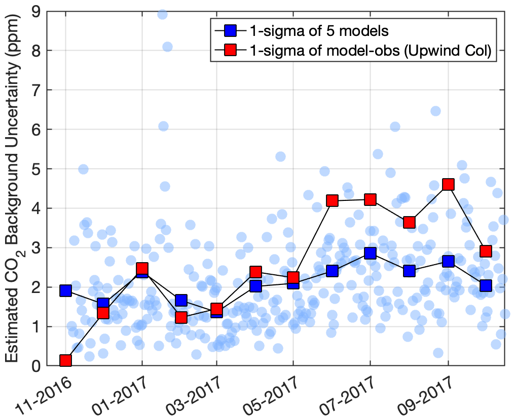
Figure 8Comparison of two methods for estimating uncertainty on CO2 background at HAL. The blue squares indicate monthly means of the standard deviation of five different backgrounds (light blue circles are daily). Red points indicate the monthly means of the standard deviation of the difference between modeled and observed mole fractions using the upwind column background during low-footprint periods. The other sites show identical patterns and very similar values.
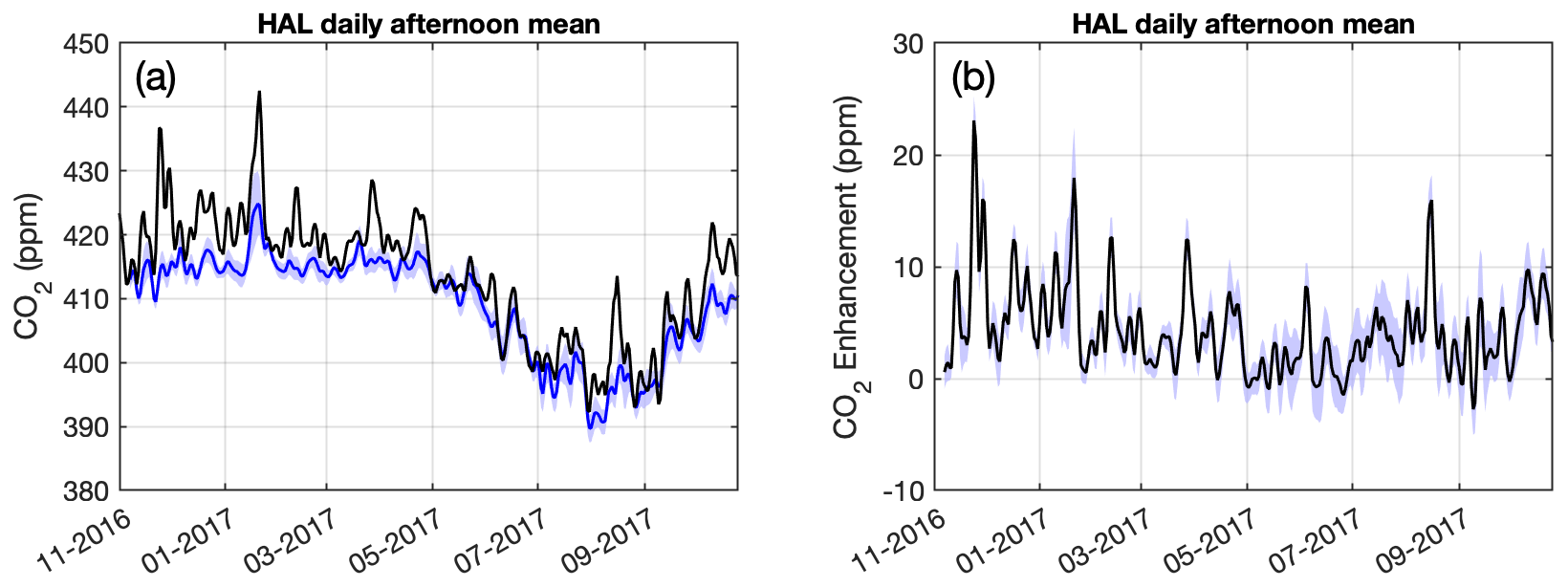
Figure 9(a) Observed CO2 time series at HAL for 1 year (black) with the background (blue) as the mean of five backgrounds from Table 1. (b) Corresponding CO2 enhancement time series. We note that in summer the enhancements can be small or even negative, because they represent the impact of both positive (anthropogenic and biogenic) and negative (biogenic) fluxes in the urban domain. In both panels, lines are the 7 d moving average of mid-afternoon daily means; blue shading indicates the standard deviation of the five backgrounds.

Figure 10(a) Monthly box plot of the hourly signal-to-noise ratio (SNR) at all sites (afternoon hours only), calculated as the CO2 enhancement (yenh) above the background divided by the standard deviation of the backgrounds (Fig. 8) for each hour. Red lines are medians; box edges indicate the 25th and 75th percentiles; whiskers indicate the extent excluding outliers, which are shown in red + marks. The y axis has been truncated for readability, so some outliers, up to 30, are not shown. (b) Average SNR by month for each site. Black solid line in both panels indicates SNR = 1.
We explore the impact of the background errors on the ability of an urban measurement station to detect a signal in CO2 enhancement. Figure 9a shows the background, chosen as the mean of the first five backgrounds we investigated in Table 1 (blue), along with observations (black), at HAL. We use the standard deviation of the five backgrounds, shown in blue circles and blue squares in Fig. 8, as a proxy for the noise, or possible error, on each hourly background mole fraction (blue shading, Fig. 9). Figure 9b shows the corresponding daily mean mid-afternoon enhancement (the background subtracted from the observed CO2 mole fraction). The signal-to-noise ratio (SNR) is calculated as the ratio between the absolute value of the enhancement and the daily mean mid-afternoon standard deviation from the five backgrounds. Figure 10a shows the SNR box plot for each month of the year for all sites together, while the mean SNR at each site is shown in Fig. 10b. The analysis indicates that through the year there are periods, mostly in late fall and winter, when the observations show a clear enhancement above the uncertainty range of the background and higher SNR. However, the median and mean SNR are low for much of the May to September time frame, because the enhancements over background are quite small during that time period, while background uncertainties are larger than in winter (Figs. 8 and 9b). Most of the loss of the SNR is driven by small summer enhancements caused by lower anthropogenic emissions that are diluted by deeper planetary boundary layers and taken up by the significant vegetation in the domain. A similar result was found in Boston (Sargent et al., 2018), where net summer enhancements were essentially zero in that similarly highly vegetated metropolitan area. We note that if the influence of urban biospheric fluxes on enhancements were removed (by using a biospheric flux model, for example), the SNR on the anthropogenic enhancements alone would be larger in summer, although that analysis would introduce errors associated with the biosphere flux modeling as well. Estimating CO2 fluxes in summer will thus be a challenge, requiring accurate modeling of both biospheric fluxes (within the domain and close to upwind sites) and meteorology to be able to overcome the uncertainty in the background conditions. The difficulty of background determination in summer is additional to the challenge of separating biospheric and anthropogenic fluxes inside the domain during the growing season.
Previous work has shown that the background conditions in the Washington/Baltimore area have significant variability in both space and time (Mueller et al., 2018), as strong upwind sources of both CO2 and CH4 influence concentrations observed at urban tower sites. Here we compare a series of model-based backgrounds as well as backgrounds derived using upwind observations. Our evaluation against observations over 1 calendar year indicates that a background concentration derived from sampling observations from an upwind tower at the same time as the urban measurement performs well in the case of CH4 and wintertime CO2 but is negatively biased in summer due to diurnally varying biogenic CO2 fluxes near upwind sites. However, we find that a similar upwind observation-based background that also accounts for vertical dispersion using a Lagrangian particle dispersion model performs best for summertime CO2 and equally well for CH4 and wintertime CO2, with little bias over the year. However, for CO2, we find that this upwind column method may not be able to entirely eliminate a summertime low bias.
In evaluating backgrounds based on sampling global or regional modeled concentrations at the edge of the domain, we found that they perform almost as well for CO2 as the best upwind observation-based background. For CH4, the conclusion is different: the less accurate regional and global modeled concentrations and the lack of strong diurnally varying biospheric fluxes near our background sites mean that using upwind observations (either using the vertical column or using same-time observations) as a background is a much better choice. Our analysis shows, however, that even when using the optimal choice of background, uncertainty in any individual hour or even month can be large, with summer mean monthly biases up to 2 ppm for CO2 with significant scatter of 1 to 3 ppm and estimated random CH4 uncertainties at 25 ppb (although this is likely an upper bound, as some of this scatter is from unknown fluxes inside the domain).
Our study allows us to give some guidance with regard to background for researchers establishing urban GHG tower networks. First, establishing stations upwind of the area of interest in a configuration that has been shown to capture incoming air from the predominant wind directions is crucial. For our network, a synthetic design study by Mueller et al. (2018) identified locations whose observations best correlated with the “true” background. Second, the best-performing background for summertime CO2 required integration of the upwind tower observations with knowledge of boundary layer height and observations in the free troposphere. We used existing free tropospheric observations from the NOAA/GML aircraft network, which provided measurements every 2 weeks at best. More frequent observations would have better captured synoptic-scale variability above the PBL and likely improved the upwind column background. Some capacity to conduct such airborne measurements should be considered in urban studies. Third, model-based backgrounds should still be considered, especially in cases where they can either be optimized in the urban inversion directly or informed by a nested inversion framework that allows upwind fluxes to be estimated rather than assumed. We did not extend our study to optimizing the modeled backgrounds using the tower observations, but it would be one way to adjust the modeled background and improve performance.
Our estimates of urban enhancement uncertainty stemming from background errors show that signal-to-noise ratios are small in the Washington/Baltimore domain, drawing attention to the fact that background errors must be accounted for in any analysis of enhancements. This finding may not apply to a different urban region, for example a city with larger anthropogenic enhancements and smaller biospheric influence both within and outside its bounds. However, we believe the methods used here to evaluate different background products and assess uncertainty are extensible and can be applied in other urban and regional studies. We specifically focus our evaluation metrics on bias, as biases will have the largest impact on posteriors from atmospheric flux inversions (as compared with random errors). We recommend evaluation of background methods for a given urban domain, as the same background methodology may not be the best-suited for a different network design, region, or trace gas of interest.
All observational data in this work are archived at https://doi.org/10.18434/M32126 (Karion et al., 2019). CMA data are available from the CO2 GLOBALVIEWplus v5.0 ObsPack (https://doi.org/10.25925/20190812) (Cooperative Global Atmospheric Data Integration Project, 2019) and the CH4 GLOBALVIEWplus v2.0 ObsPack (https://doi.org/10.25925/20200424) (Cooperative Global Atmospheric Data Integration Project, 2020).
The study was conceptualized by AK with input from KM, ILC, SMG, and SG. AK performed the investigation and analysis; data were provided by WC, EG, MS, and SP; model output was provided by ILC (transport) and SMG (VPRM). AK wrote the manuscript with review and editing by SMG, SG, ILC, KM, and JW.
The authors declare that they have no conflict of interest.
References are made to certain commercially available products in this paper to adequately specify the experimental procedures involved. Such identification does not imply recommendation or endorsement by NIST, nor does it imply that these products are the best for the purpose specified.
We are grateful for the assistance of the Earth Networks technical and engineering team, including Uran Veseshta, Clayton Fain, Bryan Biggs, Seth Baldelli, Joe Considine, and Charlie Draper, for maintaining and operating the observational tower network. We thank Jooil Kim, Peter Salameh, and Kris Verhulst for assisting with data quality and software management. This work was funded by the NIST Greenhouse Gas Measurements Program.
Support for Earth Networks provided by NIST grant numbers 70NANB15H344 and 70NANB14H322 and NIST commercial contract 1333ND19PNB600853.
This paper was edited by Ronald Cohen and reviewed by Zachary Barkley and Grant Allen.
Ammoura, L., Xueref-Remy, I., Vogel, F., Gros, V., Baudic, A., Bonsang, B., Delmotte, M., Té, Y., and Chevallier, F.: Exploiting stagnant conditions to derive robust emission ratio estimates for CO2, CO and volatile organic compounds in Paris, Atmos. Chem. Phys., 16, 15653–15664, https://doi.org/10.5194/acp-16-15653-2016, 2016.
Asefi-Najafabady, S., Rayner, P. J., Gurney, K. R., McRobert, A., Song, Y., Coltin, K., Huang, J., Elvidge, C., and Baugh, K.: A multiyear, global gridded fossil fuel CO2 emission data product: Evaluation and analysis of results, J. Geophys. Res.-Atmos., 119, 10213–210231, https://doi.org/10.1002/2013JD021296, 2014.
Balashov, N. V., Davis, K. J., Miles, N. L., Lauvaux, T., Richardson, S. J., Barkley, Z. R., and Bonin, T. A.: Background heterogeneity and other uncertainties in estimating urban methane flux: results from the Indianapolis Flux Experiment (INFLUX), Atmos. Chem. Phys., 20, 4545–4559, https://doi.org/10.5194/acp-20-4545-2020, 2020.
Barkley, Z. R., Lauvaux, T., Davis, K. J., Deng, A., Fried, A., Weibring, P., Richter, D., Walega, J. G., DiGangi, J., Ehrman, S. H., Ren, X., and Dickerson, R. R.: Estimating Methane Emissions From Underground Coal and Natural Gas Production in Southwestern Pennsylvania, Geophys. Res. Lett., 46, 4531–4540, https://doi.org/10.1029/2019gl082131, 2019.
Bréon, F. M., Broquet, G., Puygrenier, V., Chevallier, F., Xueref-Remy, I., Ramonet, M., Dieudonné, E., Lopez, M., Schmidt, M., Perrussel, O., and Ciais, P.: An attempt at estimating Paris area CO2 emissions from atmospheric concentration measurements, Atmos. Chem. Phys., 15, 1707–1724, https://doi.org/10.5194/acp-15-1707-2015, 2015.
Chen, F. and Dudhia, J.: Coupling an Advanced Land Surface–Hydrology Model with the Penn State–NCAR MM5 Modeling System. Part I: Model Implementation and Sensitivity, Mon. Weather Rev., 129, 569–585, https://doi.org/10.1175/1520-0493(2001)129<0569:Caalsh>2.0.Co;2, 2001.
Cooperative Global Atmospheric Data Integration Project: Multi-laboratory compilation of atmospheric carbon dioxide data for the period 1957–2018, obspack_co2_1_GLOBALVIEWplus_v5.0_2019_08_12, https://doi.org/10.25925/20190812, 2019.
Cooperative Global Atmospheric Data Integration Project: Multi-laboratory compilation of atmospheric methane data for the period 1957–2018; obspack_ch4_1_GLOBALVIEWplus_v2.0_2020-04-24, https://doi.org/10.25925/20200424, 2020.
Crippa, M., Guizzardi, D., Muntean, M., and Schaaf, E.: EDGAR v5.0 Global Air Pollutant Emissions, https://doi.org/10.2904/JRC_DATASET_EDGAR, 2019.
Gourdji, S., Karion, A., Lopez-Coto, I., Ghosh, S., Mueller, K. L., Zhou, Y., Williams, C. A., Baker, I. T., Haynes, K., and Whetstone, J.: A modified Vegetation Photosynthesis and Respiration Model (VPRM) for the eastern USA and Canada, evaluated with comparison to atmospheric observations and other biospheric models, J. Geophys. Res.-Biogeo., https://doi.org/10.1002/essoar.10506768.1, in review, 2021.
Gurney, K. R., Liang, J., Patarasuk, R., Song, Y., Huang, J., and Roest, G.: Vulcan: High-Resolution Annual Fossil Fuel CO2 Emissions in USA, 2010–2015, Version 3, ORNL DAAC, Oak Ridge, Tennessee, USA. https://doi.org/10.3334/ORNLDAAC/1741, 2020a.
Gurney, K. R., Liang, J., Patarasuk, R., Song, Y., Huang, J., and Roest, G.: The Vulcan Version 3.0 High-Resolution Fossil Fuel CO2 Emissions for the United States, J. Geophys. Res.-Atmos., 125, e2020JD032974, https://doi.org/10.1029/2020jd032974, 2020b.
Homer, C., Dewitz, J., Yang, L. M., Jin, S., Danielson, P., Xian, G., Coulston, J., Herold, N., Wickham, J., and Megown, K.: Completion of the 2011 National Land Cover Database for the Conterminous United States – Representing a Decade of Land Cover Change Information, Photogramm. Eng. Rem. S., 81, 345–354, 2015.
Jacobson, A. R., Schuldt, K. N., Miller, J. B., Oda, T., Tans, P., Arlyn, A., Mund, J., Ott, L., Collatz, G. J., Aalto, T., Afshar, S., Aikin, K., Aoki, S., Apadula, F., Baier, B., Bergamaschi, P., Beyersdorf, A., Biraud, S. C., Bollenbacher, A., Bowling, D., Brailsford, G., Abshire, J. B., Chen, G., Huilin, C., Lukasz, C., Sites, C., Colomb, A., Conil, S., Cox, A., Cristofanelli, P., Cuevas, E., Curcoll, R., Sloop, C. D., Davis, K., Wekker, S. D., Delmotte, M., DiGangi, J. P., Dlugokencky, E., Ehleringer, J., Elkins, J. W., Emmenegger, L., Fischer, M. L., Forster, G., Frumau, A., Galkowski, M., Gatti, L. V., Gloor, E., Griffis, T., Hammer, S., Haszpra, L., Hatakka, J., Heliasz, M., Hensen, A., Hermanssen, O., Hintsa, E., Holst, J., Jaffe, D., Karion, A., Kawa, S. R., Keeling, R., Keronen, P., Kolari, P., Kominkova, K., Kort, E., Krummel, P., Kubistin, D., Labuschagne, C., Langenfelds, R., Laurent, O., Laurila, T., Lauvaux, T., Law, B., Lee, J., Lehner, I., Leuenberger, M., Levin, I., Levula, J., Lin, J., Lindauer, M., Loh, Z., Lopez, M., Myhre, C. L., Machida, T., Mammarella, I., Manca, G., Manning, A., Manning, A., Marek, M. V., Marklund, P., Martin, M. Y., Matsueda, H., McKain, K., Meijer, H., Meinhardt, F., Miles, N., Miller, C. E., Mölder, M., Montzka, S., Moore, F., Josep-Anton, M., Morimoto, S., Munger, B., Jaroslaw, N., Newman, S., Nichol, S., Niwa, Y., O'Doherty, S., Mikaell, O.-L., Paplawsky, B., Peischl, J., Peltola, O., Jean-Marc, P., Piper, S., Plass-Dölmer, C., Ramonet, M., Reyes-Sanchez, E., Richardson, S., Riris, H., Ryerson, T., Saito, K., Sargent, M., Sasakawa, M., Sawa, Y., Say, D., Scheeren, B., Schmidt, M., Schmidt, A., Schumacher, M., Shepson, P., Shook, M., Stanley, K., Steinbacher, M., Stephens, B., Sweeney, C., Thoning, K., Torn, M., Turnbull, J., Tørseth, K., Bulk, P. V. D., Laan-Luijkx, I. T. V. D., Dinther, D. V., Vermeulen, A., Viner, B., Vitkova, G., Walker, S., Weyrauch, D., Wofsy, S., Worthy, D., Dickon, Y., and Miroslaw, Z.: CarbonTracker CT2019, https://doi.org/10.25925/39M3-6069, 2020.
Jeong, S., Newman, S., Zhang, J., Andrews, A. E., Bianco, L., Bagley, J., Cui, X., Graven, H., Kim, J., Salameh, P., LaFranchi, B. W., Priest, C., Campos-Pineda, M., Novakovskaia, E., Sloop, C. D., Michelsen, H. A., Bambha, R. P., Weiss, R. F., Keeling, R., and Fischer, M. L.: Estimating methane emissions in California's urban and rural regions using multitower observations, J. Geophys. Res.-Atmos., 121, 13031–13049, https://doi.org/10.1002/2016JD025404, 2016.
Kain, J. S.: The Kain–Fritsch Convective Parameterization: An Update, J Appl. Meteorol., 43, 170–181, https://doi.org/10.1175/1520-0450(2004)043<0170:Tkcpau>2.0.Co;2, 2004.
Karion, A., Sweeney, C., Miller, J. B., Andrews, A. E., Commane, R., Dinardo, S., Henderson, J. M., Lindaas, J., Lin, J. C., Luus, K. A., Newberger, T., Tans, P., Wofsy, S. C., Wolter, S., and Miller, C. E.: Investigating Alaskan methane and carbon dioxide fluxes using measurements from the CARVE tower, Atmos. Chem. Phys., 16, 5383–5398, https://doi.org/10.5194/acp-16-5383-2016, 2016.
Karion, A., Whetstone, J. R., Callahan, W., Prinzivalli, S., Stock, M., DiGangi, E., Fain, C., Biggs, B., Draper, C., Baldelli, S., and Considine, J.: Observations of CO2, CH4, and CO mole fractions from the NIST Northeast Corridor urban testbed, https://doi.org/10.18434/M32126, 2019.
Karion, A., Callahan, W., Stock, M., Prinzivalli, S., Verhulst, K. R., Kim, J., Salameh, P. K., Lopez-Coto, I., and Whetstone, J.: Greenhouse gas observations from the Northeast Corridor tower network, Earth Syst. Sci. Data, 12, 699–717, https://doi.org/10.5194/essd-12-699-2020, 2020.
Lauvaux, T., Miles, N. L., Deng, A. J., Richardson, S. J., Cambaliza, M. O., Davis, K. J., Gaudet, B., Gurney, K. R., Huang, J. H., O'Keefe, D., Song, Y., Karion, A., Oda, T., Patarasuk, R., Razlivanov, I., Sarmiento, D., Shepson, P., Sweeney, C., Turnbull, J., and Wu, K.: High-resolution atmospheric inversion of urban CO2 emissions during the dormant season of the Indianapolis Flux Experiment (INFLUX), J. Geophys. Res.-Atmos., 121, 5213–5236, https://doi.org/10.1002/2015jd024473, 2016.
Lauvaux, T., Gurney, K. R., Miles, N. L., Davis, K. J., Richardson, S. J., Deng, A., Nathan, B. J., Oda, T., Wang, J. A., Hutyra, L., and Turnbull, J.: Policy-Relevant Assessment of Urban CO2 Emissions, Environ. Sci. Technol., 54, 10237–10245, https://doi.org/10.1021/acs.est.0c00343, 2020.
Lin, J. C., Gerbig, C., Wofsy, S. C., Andrews, A. E., Daube, B. C., Davis, K. J., and Grainger, C. A.: A near-field tool for simulating the upstream influence of atmospheric observations: The Stochastic Time-Inverted Lagrangian Transport (STILT) model, J. Geophys. Res.-Atmos., 108, 4493, https://doi.org/10.1029/2002JD003161, 2003.
Lopez-Coto, I., Ghosh, S., Prasad, K., and Whetstone, J.: Tower-based greenhouse gas measurement network design – The National Institute of Standards and Technology North East Corridor Testbed, Adv. Atmos. Sci., 34, 1095–1105, https://doi.org/10.1007/s00376-017-6094-6, 2017.
Lopez-Coto, I., Hicks, M., Karion, A., Sakai, R. K., Demoz, B., Prasad, K., and Whetstone, J.: Assessment of Planetary Boundary Layer parametrizations and urban heat island comparison: Impacts and implications for tracer transport, J. Appl. Meteorol. Clim., 59, 1637–1653, https://doi.org/10.1175/jamc-d-19-0168.1, 2020a.
Lopez-Coto, I., Ren, X., Salmon, O. E., Karion, A., Shepson, P. B., Dickerson, R. R., Stein, A., Prasad, K., and Whetstone, J. R.: Wintertime CO2, CH4, and CO Emissions Estimation for the Washington, DC–Baltimore Metropolitan Area Using an Inverse Modeling Technique, Environ. Sci. Technol., 54, 2606–2614, https://doi.org/10.1021/acs.est.9b06619, 2020b.
Maasakkers, J. D., Jacob, D. J., Sulprizio, M. P., Turner, A. J., Weitz, M., Wirth, T., Hight, C., DeFigueiredo, M., Desai, M., Schmeltz, R., Hockstad, L., Bloom, A. A., Bowman, K. W., Jeong, S., and Fischer, M. L.: Gridded National Inventory of US Methane Emissions, Environ. Sci. Technol., 50, 13123–13133, https://doi.org/10.1021/acs.est.6b02878, 2016.
Mesinger, F., DiMego, G., Kalnay, E., Mitchell, K., Shafran, P. C., Ebisuzaki, W., Jović, D., Woollen, J., Rogers, E., Berbery, E. H., Ek, M. B., Fan, Y., Grumbine, R., Higgins, W., Li, H., Lin, Y., Manikin, G., Parrish, D., and Shi, W.: North American Regional Reanalysis, B. Am. Meteorol. Soc., 87, 343–360, https://doi.org/10.1175/bams-87-3-343, 2006.
Mitchell, L. E., Lin, J. C., Bowling, D. R., Pataki, D. E., Strong, C., Schauer, A. J., Bares, R., Bush, S. E., Stephens, B. B., Mendoza, D., Mallia, D., Holland, L., Gurney, K. R., and Ehleringer, J. R.: Long-term urban carbon dioxide observations reveal spatial and temporal dynamics related to urban characteristics and growth, P. Natl. Acad. Sci. USA, 115, 2912–2917, https://doi.org/10.1073/pnas.1702393115, 2018.
Mlawer, E. J., Taubman, S. J., Brown, P. D., Iacono, M. J., and Clough, S. A.: Radiative transfer for inhomogeneous atmospheres: RRTM, a validated correlated-k model for the longwave, J. Geophys. Res.-Atmos., 102, 16663–16682, https://doi.org/10.1029/97jd00237, 1997.
Mueller, K., Yadav, V., Lopez-Coto, I., Karion, A., Gourdji, S., Martin, C., and Whetstone, J.: Siting Background Towers to Characterize Incoming Air for Urban Greenhouse Gas Estimation: A Case Study in the Washington, DC/Baltimore Area, J. Geophys. Res.-Atmos., 123, 2910–2926, https://doi.org/10.1002/2017JD027364, 2018.
Nakanishi, M. and Niino, H.: An Improved Mellor–Yamada Level-3 Model with Condensation Physics: Its Design and Verification, Bound.-Lay. Meteorol., 112, 1–31, https://doi.org/10.1023/B:BOUN.0000020164.04146.98, 2004.
Nakanishi, M. and Niino, H.: An Improved Mellor–Yamada Level-3 Model: Its Numerical Stability and Application to a Regional Prediction of Advection Fog, Bound.-Lay. Meteorol., 119, 397–407, https://doi.org/10.1007/s10546-005-9030-8, 2006.
Nickless, A., Rayner, P. J., Engelbrecht, F., Brunke, E.-G., Erni, B., and Scholes, R. J.: Estimates of CO2 fluxes over the city of Cape Town, South Africa, through Bayesian inverse modelling, Atmos. Chem. Phys., 18, 4765–4801, https://doi.org/10.5194/acp-18-4765-2018, 2018.
Olson, J. B., Kenyon, J. S., Angevine, W. A., Brown, J. M., Pagowski, M., and Sušelj, K.: A Description of the MYNN-EDMF Scheme and the Coupling to Other Components in WRF–ARW, Technical Memorandum, Boulder, CO, https://doi.org/10.25923/n9wm-be49, 2019.
Peters, W., Jacobson, A. R., Sweeney, C., Andrews, A. E., Conway, T. J., Masarie, K., Miller, J. B., Bruhwiler, L. M. P., Petron, G., Hirsch, A. I., Worthy, D. E. J., van der Werf, G. R., Randerson, J. T., Wennberg, P. O., Krol, M. C., and Tans, P. P.: An atmospheric perspective on North American carbon dioxide exchange: CarbonTracker, P. Natl. Acad. Sci. USA, 104, 18925–18930, https://doi.org/10.1073/pnas.0708986104, 2007.
Peters, W., Krol, M. C., Van Der Werf, G. R., Houweling, S., Jones, C. D., Hughes, J., Schaefer, K., Masarie, K. A., Jacobson, A. R., Miller, J. B., Cho, C. H., Ramonet, M., Schmidt, M., Ciattaglia, L., Apadula, F., Heltai, D., Meinhardt, F., Di Sarra, A. G., Piacentino, S., Sferlazzo, D., Aalto, T., Hatakka, J., Strom, J., Haszpra, L., Meijer, H. A. J., Van Der Laan, S., Neubert, R. E. M., Jordan, A., Rodo, X., Morgui, J.-A., Vermeulen, A. T., Popa, E., Rozanski, K., Zimnoch, M., Manning, A. C., Leuenberger, M., Uglietti, C., Dolman, A. J., Ciais, P., Heimann, M., and Tans, P. P.: Seven years of recent European net terrestrial carbon dioxide exchange constrained by atmospheric observations, Glob. Change Biol., 16, 1317–1337, https://doi.org/10.1111/j.1365-2486.2009.02078.x, 2010.
Sargent, M., Barrera, Y., Nehrkorn, T., Hutyra, L. R., Gately, C. K., Jones, T., McKain, K., Sweeney, C., Hegarty, J., Hardiman, B., Wang, J. A., and Wofsy, S. C.: Anthropogenic and biogenic CO2 fluxes in the Boston urban region, P. Natl. Acad. Sci. USA, 115, 7491–7496, https://doi.org/10.1073/pnas.1803715115, 2018.
Segers, A. and Houweling, S.: Validation of the CH4 surface flux inversion – reanalysis 1990–2017, Copernicus Atmosphere Monitoring Service, Shinfield Park, Reading, UK, CAMS73_2015SC3_D73.2.4.4-2017_201811_validation_CH4_1990-2017_v1, 2018.
Shusterman, A. A., Teige, V. E., Turner, A. J., Newman, C., Kim, J., and Cohen, R. C.: The BErkeley Atmospheric CO2 Observation Network: initial evaluation, Atmos. Chem. Phys., 16, 13449–13463, https://doi.org/10.5194/acp-16-13449-2016, 2016.
Sweeney, C., Karion, A., Wolter, S., Newberger, T., Guenther, D., Higgs, J. A., Andrews, A. E., Lang, P. M., Neff, D., and Dlugokencky, E.: Seasonal climatology of CO2 across North America from aircraft measurements in the NOAA/ESRL Global Greenhouse Gas Reference Network, J. Geophys. Res.-Atmos., 120, 5155–5190, 2015.
Taylor, K. E.: Summarizing multiple aspects of model performance in a single diagram, J. Geophys. Res.-Atmos., 106, 7183–7192, https://doi.org/10.1029/2000jd900719, 2001.
Thompson, G., Rasmussen, R. M., and Manning, K.: Explicit Forecasts of Winter Precipitation Using an Improved Bulk Microphysics Scheme. Part I: Description and Sensitivity Analysis, Mon. Weather Rev., 132, 519–542, https://doi.org/10.1175/1520-0493(2004)132<0519:Efowpu>2.0.Co;2, 2004.
Thompson, G., Field, P. R., Rasmussen, R. M., and Hall, W. D.: Explicit Forecasts of Winter Precipitation Using an Improved Bulk Microphysics Scheme. Part II: Implementation of a New Snow Parameterization, Mon. Weather Rev., 136, 5095–5115, https://doi.org/10.1175/2008mwr2387.1, 2008.
Thoning, K. W., Tans, P. P., and Komhyr, W. D.: Atmospheric Carbon Dioxide at Mauna Loa Observatory 2. Analysis of the NOAA GMCC Data, 1974–1985, J. Geophys. Res.-Atmos., 94, 8549–8565, https://doi.org/10.1029/JD094iD06p08549, 1989.
Verhulst, K. R., Karion, A., Kim, J., Salameh, P. K., Keeling, R. F., Newman, S., Miller, J., Sloop, C., Pongetti, T., Rao, P., Wong, C., Hopkins, F. M., Yadav, V., Weiss, R. F., Duren, R. M., and Miller, C. E.: Carbon dioxide and methane measurements from the Los Angeles Megacity Carbon Project – Part 1: calibration, urban enhancements, and uncertainty estimates, Atmos. Chem. Phys., 17, 8313–8341, https://doi.org/10.5194/acp-17-8313-2017, 2017.
Xueref-Remy, I., Dieudonné, E., Vuillemin, C., Lopez, M., Lac, C., Schmidt, M., Delmotte, M., Chevallier, F., Ravetta, F., Perrussel, O., Ciais, P., Bréon, F.-M., Broquet, G., Ramonet, M., Spain, T. G., and Ampe, C.: Diurnal, synoptic and seasonal variability of atmospheric CO2 in the Paris megacity area, Atmos. Chem. Phys., 18, 3335–3362, https://doi.org/10.5194/acp-18-3335-2018, 2018.
Zhou, Y., Williams, C. A., Lauvaux, T., Davis, K. J., Feng, S., Baker, I., Denning, S., and Wei, Y. X.: A Multiyear Gridded Data Ensemble of Surface Biogenic Carbon Fluxes for North America: Evaluation and Analysis of Results, J. Geophys. Res.-Biogeo., 125, e2019JG005314, https://doi.org/10.1029/2019jg005314, 2020.
- Abstract
- Introduction
- Methods
- Synthetic experiment evaluation of upwind observation-based CO2 backgrounds
- Evaluation of CO2 and CH4 background performance using urban tower observations
- Discussion
- Conclusions
- Data availability
- Author contributions
- Competing interests
- Disclaimer
- Acknowledgements
- Financial support
- Review statement
- References