the Creative Commons Attribution 4.0 License.
the Creative Commons Attribution 4.0 License.
 | 19 Apr 2021
How Asian aerosols impact regional surface temperatures across the globe
Kalle Nordling
Petri Räisänen
Jouni Räisänen
Declan O'Donnell
Antti-Ilari Partanen
Hannele Korhonen
South and East Asian anthropogenic aerosols mostly reside in an air mass extending from the Indian Ocean to the North Pacific. Yet the surface temperature effects of Asian aerosols spread across the whole globe. Here, we remove Asian anthropogenic aerosols from two independent climate models (ECHAM6.1 and NorESM1) using the same representation of aerosols via MACv2-SP (a simple plume implementation of the second version of the Max Planck Institute Aerosol Climatology). We then robustly decompose the global distribution of surface temperature responses into contributions from atmospheric energy flux changes. We find that the horizontal atmospheric energy transport strongly moderates the surface temperature response over the regions where Asian aerosols reside. Atmospheric energy transport and changes in clear-sky longwave radiation redistribute the temperature effects efficiently across the Northern Hemisphere and to a lesser extent also over the Southern Hemisphere. The model-mean global surface temperature response to Asian anthropogenic aerosol removal is 0.26±0.04 ∘C (0.22±0.03 for ECHAM6.1 and 0.30±0.03 ∘C for NorESM1) of warming. Model-to-model differences in global surface temperature response mainly arise from differences in longwave cloud (0.01±0.01 for ECHAM6.1 and 0.05±0.01 ∘C for NorESM1) and shortwave cloud (0.03±0.03 for ECHAM6.1 and 0.07±0.02 ∘C for NorESM1) responses. The differences in cloud responses between the models also dominate the differences in regional temperature responses. In both models, the northern-hemispheric surface warming amplifies towards the Arctic, where the total temperature response is highly seasonal and weakest during the Arctic summer. We estimate that under a strong Asian aerosol mitigation policy tied with strong climate mitigation (Shared Socioeconomic Pathway 1-1.9) the Asian aerosol reductions can add around 8 years' worth of current-day global warming during the next few decades.
- Article
(18491 KB) - Full-text XML
- BibTeX
- EndNote


Understanding how regional climates respond to different climate forcers is crucial for assessing how climate change impacts societies. Samset et al. (2018) showed that anthropogenic aerosols cool the global-mean surface temperature in four latest-generation climate models by between 0.5–1.1 K. However, the regional impacts of anthropogenic aerosols on surface temperatures remain particularly complicated to unravel (Persad and Caldeira, 2018; Nordling et al., 2019).
Due to the short lifetime of aerosols, their distribution in the atmosphere is highly heterogeneous and dependent on the location of their emissions and on various dynamical and microphysical processes influencing also their properties and climate effects. Aerosols give rise to both local and remote temperature responses, so that the geographic distributions of aerosol radiative forcing and temperature effects are largely dislocated (Shindell et al., 2010; Nordling at al., 2019). Furthermore, the same aerosol emissions originating from different regions vary in their climate forcing efficacies, with their global surface temperature response per unit global radiative forcing differing by factors of between 2 and 14, depending on aerosols species and the models used (Kasoar et al., 2018; Westervelt, et al., 2020; Persad and Caldeira, 2018).
During the past decades air pollution levels in Europe and North America have decreased considerably, while they have grown in South and East Asia. These opposing changes in air pollution have kept the overall global anthropogenic aerosol radiative forcing close to constant since the mid-1970s (Murphy 2013; Fiedler et al., 2019). South and East Asia have become the dominant sources of anthropogenic aerosol emissions (Lamarque et al., 2010). Consequently, air pollution has become a major health problem in Asia. Ambient aerosol pollution reduces the life expectancy by 1.24 years in East Asia and by 1.56 years in South Asia (Apte et al., 2018) and is attributable to 0.67 million deaths per year in India alone (Balakrishnan et al., 2019). Shared Socioeconomic Pathways (SSPs) predict that strong air pollution mitigation policies (SSP1-1.9) could reduce the Asian anthropogenic aerosol emissions from their 2015 levels by 55 % already by 2030 and by 90 % by 2100 (Lund et al., 2019, see also their Fig. S2).
Large past changes and potentially at least equally significant future changes in Asian aerosols have prompted recent studies on their global and regional surface temperature effects. Kasoar et al. (2016) used three climate models (HadGEM3-GA4, CESM1, and GISS-E2) to study regional surface temperature responses to the removal of SO2 emissions from China. Two of the three models showed northern-hemispheric warming due to aerosol removal but of significantly different magnitude, while the third model showed no significant surface temperature responses. The authors pinpointed the mixed results from the models to their different treatments of aerosol microphysical processes and aerosol–cloud interactions. Westervelt et al. (2020) also used three climate models (GFDL, CESM1, and GISS-E2) to investigate the surface temperature responses to the removals (or significant reductions) of aerosol sources from several different regions, including China and India. Overall, the models varied in aerosol radiative forcings and regional temperature response patterns associated with Asian aerosol reductions but suggested that the reductions mostly result in a significant surface temperature increase across the Northern Hemisphere and particularly over the Arctic. Persad and Caldeira (2018) used the CAM5 model to place an equivalent to China's total annual year 2000 anthropogenic aerosol emissions at different locations around the globe. They found that emissions placed in China cooled the whole Northern Hemisphere, while the same emissions placed in India resulted in a mixed regional response of warming and cooling.
Recent studies have also investigated the combined impacts of Asian anthropogenic aerosols on precipitation and surface temperatures. Liu et al. (2018) showed that the temperature effects of idealized Asian aerosol perturbations spread across the Northern Hemisphere in a multi-model Precipitation Driver and Response Model Intercomparison Project (PDRMIP) study. They also showed that increases in Asian sulfate aerosols strongly suppressed Asian monsoon precipitation by enhancing horizontal atmospheric heat transport to the region and raising surface pressure. Wilcox et al. (2020) showed that future reductions in global aerosol emissions, dominated by changes in Asian aerosol emissions, lead to accelerated increases in Asian monsoon precipitation in CMIP6 experiments but had a limited impact on projected future changes in surface temperatures.
Here, we explore the global and regional surface temperature responses to a complete removal of South and East Asian anthropogenic aerosols using two different climate models, ECHAM6.1 and NorESM1. As in Nordling et al. (2019), we use an identical description of anthropogenic aerosols in both models. The use of identical aerosols across the models allows us to study the similarities and differences in model dynamical responses to aerosols and exclude the model response perturbations that result from differences in modeled aerosols. Further, we aim to understand the robustness of changes in the climate system that lead to the local and remote changes in surface temperatures.
It is complicated to resolve the pathway from a climate forcing to a regional surface temperature response in climate models even for globally homogeneous greenhouse gases, let alone for aerosols. A significant climate perturbation results in a complex set of responses in general circulation patterns, cloud properties, surface albedo, atmospheric water vapor concentrations, et cetera. Surface temperature responses result from a combination of all these different climate feedbacks. Therefore, even a seemingly robust regional surface temperature signal in different climate models may result from a different combination of feedbacks that sums up to a similar temperature response.
Räisänen (2017) presented a new method built around the concept of effective planetary emissivity for a robust decomposition of the energetic components that sum up to the geographic distribution of surface temperature responses. Here, we extend the method to better resolve the longwave cloud feedback using radiative kernels and apply it for the analysis of the model results. The method allows separating the contributions from atmospheric heat transport, changes in shortwave and longwave radiation related to clear sky and clouds, surface energy fluxes, and surface albedo to a local surface temperature response.
2.1 Model experiments and analysis
We use ECHAM6.1 (Stevens et al., 2013) and NorESM1 (Bentsen et al., 2013; Iversen et al., 2013; Kirkevåg et al., 2013) general circulation models to carry out 100-year slab ocean equilibrium runs for the present-day (year 2005) atmosphere without South and East Asian anthropogenic aerosols, but leaving all other aerosol sources intact. The last 60 years of equilibrated climate data from each simulation are used for the analysis. These runs are compared to otherwise identical baseline climate runs of same length but having all aerosol sources on. For the baseline, we use the same ECHAM6.1 and NorESM1 model runs as presented in Nordling et al. (2019).
The background pre-industrial aerosols (mainly consisting of natural organics and sulfate, sea salt, and dust) for ECHAM6.1 are prescribed using the climatology of Kinne et al. (2013), while for NorESM1, they are simulated by the model's bottom-up aerosol microphysics scheme (Kirkevåg et al., 2013) (see also Fig. 2 and Appendix A in Fiedler et al., 2019, describing the pre-industrial aerosols for both of the applied models and the related discussion within). In both cases, the impact of modern-day (year 2005) anthropogenic aerosols is represented via the MACv2-SP climatology (Stevens et al., 2017). MACv2-SP uses in situ observations of aerosol optical depth (AOD) for the top-to-bottom representation of aerosol-radiation effects and calculates the aerosol direct and first indirect effects through changes in fixed three-dimensional AOD fields with monthly time resolution. The anthropogenic impact on AOD is represented through nine different aerosol plumes, which together represent the sources and transport of anthropogenic aerosols, including biomass burning. In the runs without Asian anthropogenic aerosols we have turned off plume numbers 3 and 4. The direct and indirect instantaneous aerosol radiative forcings are calculated online in the models using double radiation calls. The global instantaneous forcing can be modeled nearly identically with MACv2-SP in ECHAM6.1 and NorESM1, albeit there are some model-to-model differences related to model-specific representations of clouds, surface albedo, and natural aerosol (Nordling et al., 2019). The effective radiative forcing (analyzed by Fiedler et al., 2019, for multi-decadal fixed-sea-surface-temperature runs for ECHAM6.3 and NorESM1 models using the same pre-industrial aerosol representations as here) shows somewhat larger model-to-model variations, but the geographic patterns of the effective radiative forcings with MACv2-SP are close to those of instantaneous radiative forcings. The differences in global anthropogenic aerosol radiative forcings between the ECHAM6.1 and NorESM1 models with MACv2-SP aerosols are small enough to be insignificant for the obtained temperature responses, as discussed in Nordling et al. (2019). However, different representations of natural background aerosol in the models can lead to differences in obtained indirect aerosol forcing (Carslaw et al., 2013; Fiedler et al., 2019), and this is the case also for Asian anthropogenic aerosols when using the model-intrinsic pre-industrial aerosol representations in NorESM1 and ECHAM6.1, as we will discuss later. Here, both models were coupled to their intrinsic mixed-layer (slab) ocean model representations (for ECHAM6.1 see Roeckner et al., 2003; for NorESM1 see Bitz et al., 2012), and hence changes in ocean currents are not accounted for in our analysis. The reported equilibrium climate sensitivity is 3.5 K for NorESM1 (Räisänen et al., 2017) and also 3.5 K for ECHAM6.1 (Mauritsen and Roeckner, 2020).
The analysis of results is based on monthly-mean values of data, calculated separately for each month in the 60-year time series. The response uncertainties in global-mean values are calculated as standard error of means using a 95 % confidence interval for individual models and as a pooled standard error of the mean with a 95 % confidence interval for responses averaged over the two models. The statistical significance of regional responses is evaluated using a Student's t test with an autocorrelation correction according to Zwiers and von Storch (1995).
2.2 Temperature response decomposition
We decompose the distribution of local surface temperature responses to local changes in atmospheric energetic components using a method presented in Räisänen (2017). The method only requires standardly archived climate model output for the decomposition.
The rate of change of total energy in an atmospheric column is
where is the net incoming shortwave radiation and is the outgoing longwave radiation at the top of the atmosphere, C→ is the net horizontal heat transport into the column, and the net downward heat flux into the surface is given by
where and are the net shortwave and longwave radiation fluxes into the surface, and SH↑ and LH↑ are the upwards sensible and latent heat fluxes, respectively. To relate Eq. (1) with the surface air temperature T one defines (Räisänen and Ylhäisi, 2015; Räisänen, 2017)
where the effective planetary emissivity εeff is essentially a measure of the local atmospheric greenhouse effect. Substituting Eq. (3) into Eq. (1) gives
Then, letting [] mark the mean state between baseline and perturbed climates, the change in Eq. (4) between the two climate states can be written as
Linearizing the left-hand side of Eq. (5) as
allows the decomposition of surface temperature response into changes in energy flux components in the atmospheric column,
where
We mark the surface temperature change due to horizontal heat transport and the change in the energy storage (Eq. 8d) collectively as CONV, as together they represent the convergence of energy. Annually, the change in the energy storage of an atmospheric column averages to zero in an equilibrium climate (Porter et al., 2010; Räisänen, 2017), and Eq. (8d) corresponds to the difference in horizontal heat transport between two equilibrium climates. However, on monthly and seasonal timescales the changes in atmospheric energy storage can be significant.
The terms on the right-hand side of Eq. (8a) and (8b) can be further expanded to separate the surface temperature responses due to clear-sky and cloud radiative effects. The standard climate model output contains radiative fluxes both for all-sky and clear-sky (CS) conditions, so that the temperature response to longwave cloud radiative effect can be obtained as
Räisänen (2017) calculated the surface temperature response due to changes in longwave cloud emissivity as but noted that it is a negatively biased approximation of the actual cloud longwave feedback, as also discussed by Soden et al. (2004). Here, we extend the calculation to allow for a more precise separation of thermal radiation to its clear-sky and cloud contributions with the help of radiative kernels. Radiative kernels are climate-model-derived radiative responses to small changes in climate state, such as to changes in atmospheric temperature, surface temperature, or water vapor under clear-sky and all-sky conditions. We use the radiative kernels of Block and Mauritsen (2013) and their Eq. (4) to calculate a corrected longwave cloud feedback , namely
where KT and Kw are different model level mass-weighted radiative kernels, q is the specific humidity, and the summations are carried over the model levels i. Block and Mauritsen (2013) generated their radiative kernels with the ECHAM6 climate model, and here we apply the kernels both to the ECHAM6.1 and NorESM1 models. This should bring no major bias for the NorESM1 calculations, as Myhre et al. (2018) showed that radiative kernels do not significantly depend on the specific model used for their construction. The calculated correction is used to redistribute the effect of Δεeff between the cloud and clear-sky terms as
where and are the corrected longwave cloud and clear-sky temperature responses.
As discussed in Räisänen (2017), the top-of-atmosphere shortwave radiative responses for clear-sky and all-sky conditions can also be further separated to physically more meaningful terms using the approximative partial radiative perturbation (APRP) method of Taylor et al. (2007).
where corresponds to changes in incoming solar radiation (zero in our model experiments), is the corrected clear-sky shortwave temperature response, is the shortwave cloud response, is the temperature response due to changes in surface albedo, and is a non-linear correction term, small enough to be insignificant for the analysis.
Hereafter, we use the subscripts in ΔT terms as shorthand notations when discussing the various temperature responses (so that is discussed as SWclr etc.).
3.1 Radiative forcing
Figure 1 shows the net change in instantaneous top-of-atmosphere aerosol radiative forcing, ΔIRF, due to removal of South and East Asian anthropogenic aerosols, calculated as an average over the full 60-year equilibrated climate data sets over both models as
Note that since we here remove the Asian anthropogenic aerosols from the models, ΔIRF is positive in sign, i.e., that of warming. ΔIRF further breaks into , where ΔIRFd describes the change in aerosol direct radiative forcing due to the net change in direct radiation attenuation of aerosols through their scattering and absorption of solar radiation. ΔIRFid is the change in indirect radiative forcing (the Twomey effect) between the runs without and with South and East Asian anthropogenic aerosols. The geographical pattern of ΔIRF is nearly identical for ECHAM6.1 and NorESM1, with the model-to-model correlation coefficient of 0.99. However, the modeled globally averaged ΔIRF differs slightly between the models, being 0.38±0.00 W m−2 for ECHAM6.1 and 0.41±0.00 W m−2 for NorESM1, with a model mean of 0.40±0.00 W m−2. Results for individual models are shown in the Appendix Fig. A1.
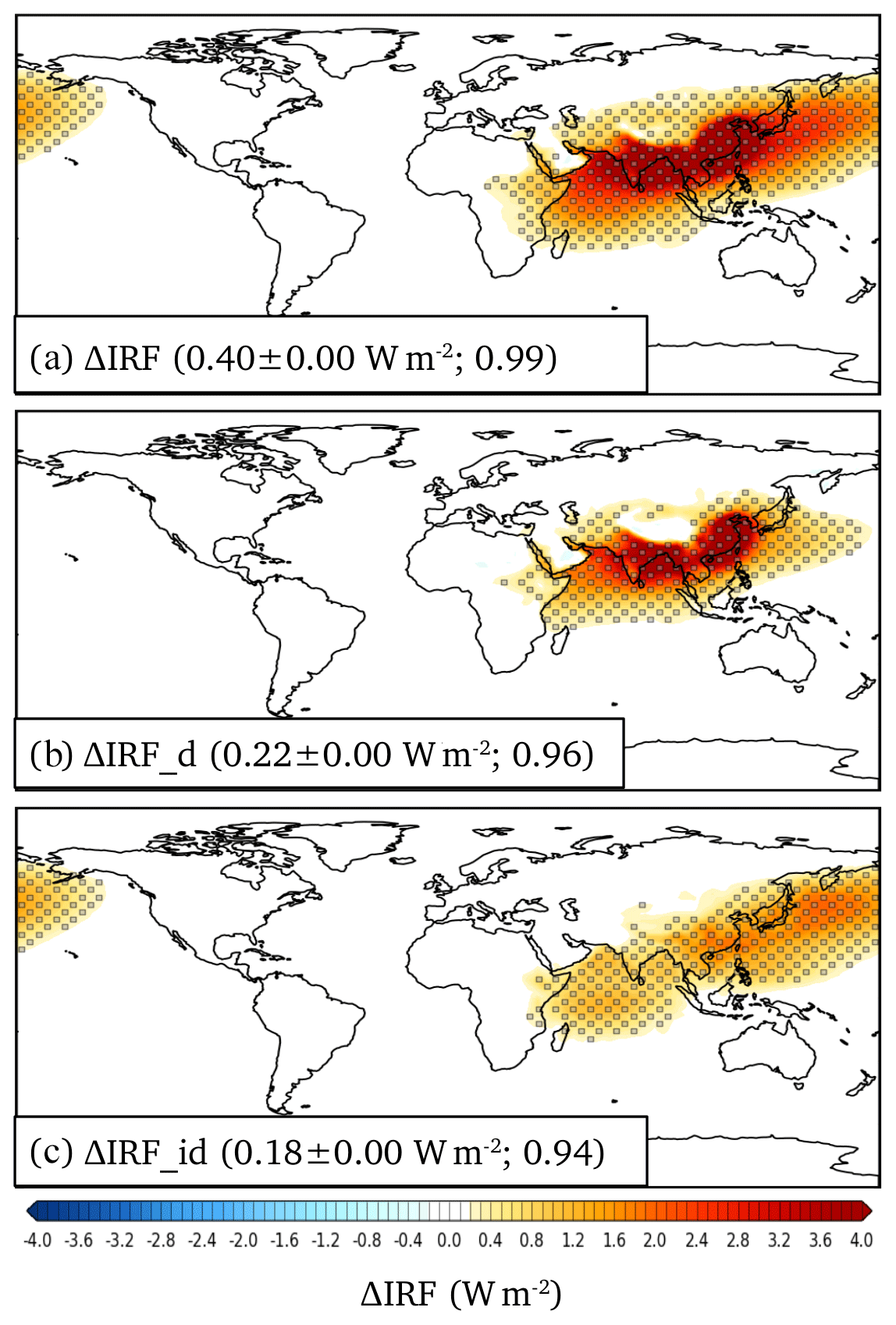
Figure 1The change in the mean instantaneous radiative forcing between runs without and with South and East Asian aerosols using the MACv2-SP aerosol scheme, averaged over the two climate models (individual models shown in Fig. A1). Parentheses show the average global-mean value and the model-to-model correlation coefficient, respectively. (a) Change in the total aerosol radiative forcing, (b) change in the direct aerosol radiative forcing, and (c) change in the indirect aerosol radiative forcing. Stippling shows regions where the results are statistically significant at the p<0.05 level for both models, and models also agree on the sign.
In the models, ΔIRF due to removal of Asian anthropogenic aerosols is concentrated on a distinctive patch over the region surrounding the aerosol sources. The change in local radiative forcing reaches up to 8.3 W m−2 over SE China. The change in direct radiative forcing ΔIRFd in the models is responsible for slightly over a half (0.22±0.00; 0.23±0.00 W m−2 for ECHAM6.1 and 0.20±0.00 W m−2 for NorESM1 with a model-to-model correlation coefficient 0.96) of the total globally averaged ΔIRF and more focused on the polluted regions than the change in indirect forcing ΔIRFid (0.18±0.00; 0.15±0.00 W m−2 for ECHAM6.1 and 0.21±0.00 W m−2 for NorESM1 with a model-to-model correlation coefficient 0.94), which spreads more evenly over a larger area. The higher model-to-model correlation coefficient for ΔIRF than for ΔIRFd and ΔIRFid separately indicates a cancellation of regional model-to-model differences when changes in direct and indirect radiative forcings are summed up. This cancellation of differences in ΔIRF suggests that differences in modeled cloud fields mainly distribute ΔIRF differently to its ΔIRFd and ΔIRFid components in the models. While the aerosols enhance the cloud albedo, clouds also diminish the direct reflection of sunlight by aerosols with compensating effects on the total radiative response. However, differences in modeled pre-industrial background aerosols likely also play a role in model-to-model difference in ΔIRFid.
3.2 Annually averaged temperature response decomposition
We first describe the commonalities in modeled surface temperature responses to the omission of South and East Asian aerosols in the two models, before discussing their differences. The average global equilibrium temperature response ΔT to the removal of aerosols across the two models is shown in Fig. 2A (individual models are shown in Figs. A2a and A3a, and global-level results are collected on Table A1). The regional distribution of surface temperature response is strikingly different from the distribution of South and East Asian anthropogenic aerosol forcing, with surface warming spreading over the entire Northern Hemisphere and to a lesser extent also to the Southern Hemisphere. Indeed, significant warming extends to regions where no change in aerosols is modeled, such as over to the North American continent (0.5 K), and to Arctic regions with warming exceeding 1 K. The warming over the region with the strongest change in local aerosol forcing (SE China) is 1.5 K with a local climate sensitivity of 0.18 K W−1 m2 (i.e., ), while the globally averaged warming is 0.26±0.04 K with a climate sensitivity of 0.65±0.11K W−1 m2). A similar global climate sensitivity of 0.58±0.23 K W−1 m2) for a 10-fold increase in Asian sulfate aerosols was found in models that participated to the multi-model intercomparison project PDRMIP (Liu et al., 2018).
As described in the Method section (Sect. 2), the total local temperature response can be represented as a sum of responses in clear and cloudy-sky shortwave (SWclr and SWcld) and longwave (LWclr and LWcld) radiation, surface albedo (ALBEDO), surface energy fluxes (SURF), and an energy convergence term (CONV) representing the horizontal transport of heat for annually averaged results. The annually averaged temperature responses for each of the energetic terms, averaged over the 60-year sets of equilibrated climate runs with both models, are shown in Fig. 2b–h. The sum of surface temperature responses to individual energetic terms (sum over Fig. 2b–h) reproduces the total surface temperature response in Fig. 2a with a spatial correlation coefficient cc=0.998 and an identical global mean.

Figure 2The geographical distributions of annually averaged surface air (2 m) temperature responses due to the removal of South and East Asian aerosols (mean over ECHAM6.1 and NorESM1 climate models). Brackets show global average responses in kelvins and the model-to-model correlation coefficient, respectively. (a) The total surface temperature response. (b–h) Contributions to the total surface temperature response from shortwave clear-sky response (b), horizontal atmospheric heat transport (c), shortwave cloud response (d), longwave cloud response (e), surface albedo change (f), longwave clear-sky response (g), and surface energy flux change (h). (b–h) Sum up to the response seen in panel (a). Panel (i) shows the combined shortwave and longwave cloud response. Stippling shows regions where the results are statistically significant at the p<0.05 level for both models, and models also agree on the sign.
First it can be noted that the geographical distribution of temperature responses due to changes in clear-sky shortwave radiation, SWclr (Fig. 2b), resembles closely the distribution of shortwave direct radiative forcing, ΔIRFd (Fig. 1b), with a correlation coefficient cc=0.96. SWclr is also one of the major energetic terms of the total globally averaged temperature response, responsible for 0.08±0.01 K of the total globally averaged temperature response of 0.26±0.04 K.
Over the whole region of positive radiative forcing (ΔIRF in Fig. 1a) the warming is moderated by the cooling caused by the transport of energy away from the region, CONV (Fig. 2c). CONV also efficiently redistributes the temperature effects across the globe. Since CONV only acts by horizontally redistributing atmospheric energy, its effect on the global surface temperature response is effectively zero ( K).
Unlike for the connection between SWclr and ΔIRFd, the geographical distribution of temperature responses due to changes in cloudy-sky shortwave radiation, SWcld (Fig. 2d) corresponds only weakly to the geographical distribution of the change in shortwave cloud radiative forcing ΔIRFid (Fig. 1c) (cc=0.23). Indeed, while there is a pronounced positive ΔIRFid in South Asia and the western subtropical North Pacific in Fig. 1c, much of the warming response in this region appears actually in the LWcld term (Fig. 2e). This is because of feedbacks that lead to changes in cloud cover and other cloud properties. Clouds both reflect SW radiation and reduce outgoing longwave radiation (e.g., Loeb et al., 2018), and changes in cloud amount tend to have opposing effects on SWcld and LWcld. The average total cloud cover change in the models is shown in Fig. 3a. The global distribution of cloud cover changes correlates strongly with LWcld (cc=0.77) and anti-correlates with SWcld (). Only by summing SWcld and LWcld (Fig. 2i) one can again recognize the warming response to ΔIRFid (Fig. 1c) (cc=0.70). There is a marked and statistically significant increase in cloud cover over India, Mainland Southeast Asia, and the western subtropical North Pacific, accompanied by a strong decrease in SWcld and increase in LWcld. The strong increase in cloud cover over India and Mainland Southeast Asia leads to a weaker overall surface temperature response (Fig. 2a) in these regions. In contrast, the decrease in cloud cover over East Asia amplifies the temperature response over the region. Further, the changes in clouds also contribute to remote temperature responses, such as to a weakening of the cloud cover over the Mediterranean and central Asia with compensating surface temperature effects from the SWcld and LWcld pathways. Overall, the combined effect of clouds (SWcld+LWcld) on the globally averaged temperature response is 0.08±0.04 K.
Together with the horizontal energy transport CONV, also the clear-sky longwave response LWclr acts as a strong redistributor of the surface temperature changes across the globe. Similarly to CO2 forcing (Räisänen, 2017), LWclr (0.08±0.03 K) is one of the major terms in the overall global temperature response also for aerosols. This is somewhat counterintuitive, as the modeled aerosols only impact the shortwave radiation in clear and cloudy skies. The geographical distribution of LWclr mainly results from a combination of atmospheric water vapor and lapse rate feedbacks (Pithan and Mauritsen, 2014; Räisänen, 2017), but the separation of these feedbacks is not pursued in this study.
Figure 2f shows the annual average change across both models in ALBEDO, that is, the surface temperature response to the change in surface albedo. The change in surface albedo is related to changes in snow and sea ice cover, but interestingly the surface albedo (ratio between reflected and incoming surface shortwave radiation) also changes over India in both models, likely due to changes in the ratio of direct vs. diffuse solar radiation. The surface albedo change further pushes the geographical distribution of warming towards northern latitudes. The globally averaged temperature effect of the surface albedo change is nevertheless small (0.02±0.01 K).
The annually averaged temperature response due to changes in surface energy flux, SURF (Fig. 2g), is zero over the continents as there is no net annual exchange of heat between continental surface and the atmosphere regardless of climate state and nonzero mainly over ocean regions where there are changes in sea ice cover. In climate runs with fully coupled ocean models, instead of slab ocean models used here, the annually averaged oceanic surface terms could be larger due to changes in oceanic circulation and heat transport. Since we have run the modeled climates to an equilibrium, the yearly averaged global SURF is zero (0.00±0.04 K); yet, it introduces a significant noise term in the results. However, the oceanic SURF term plays an important role in the seasonal cycle of regional temperature responses, as we will discuss further when describing the seasonality of modeled temperature responses.
3.3 Model-to-model differences in regional temperature responses
The parentheses in Figs. 1, 2, and 3 show the model-to-model correlation coefficients for the geographical distributions of changes in radiative forcings, temperature response terms, and cloud cover due to the removal of South and East Asian anthropogenic aerosols. The coefficients describe the geographical uniformity of responses for the ECHAM6.1 and NorESM1 climate models using the same representation of anthropogenic aerosols via the MACv2-SP aerosol scheme.
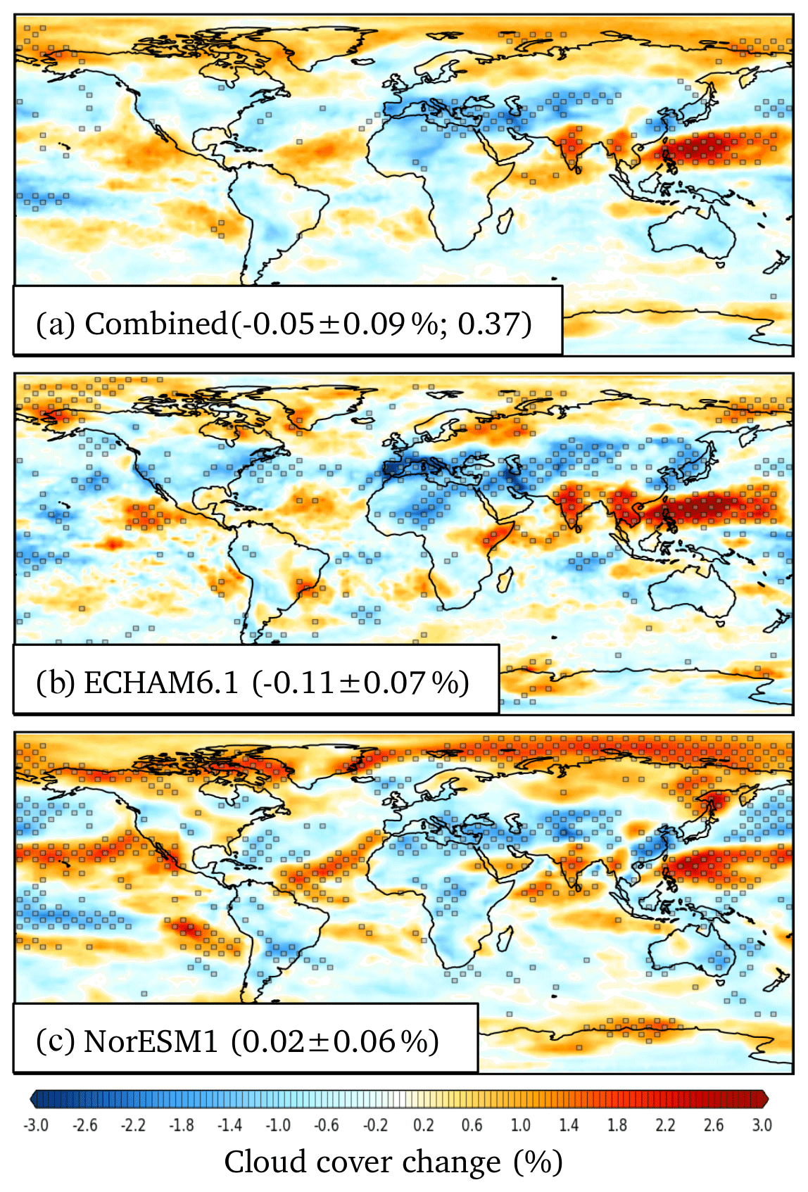
Figure 3The geographical distributions of annually averaged changes in total cloud cover due to the removal of South and East Asian aerosols. (a) Cloud cover change averaged over both ECHAM6.1 and NorESM1 climate models. Brackets show global average responses in percentages and the model-to-model correlation coefficient, respectively. Stippling shows regions where the results are statistically significant at the p<0.05 level for both models, and models also agree on the sign. (b, c) Cloud cover change in ECHAM6.1 and NorESM1, respectively. Brackets give global average responses in percentages. Stippling shows regions where the results are statistically significant at the p<0.05 level.
The strong correlation between modeled change in aerosol direct radiative forcing ΔIRFd (cc=0.96) translates into a strong correlation between the modeled surface temperature response due to SWclr (cc=0.91). However, the strong correlation for the change in aerosol indirect radiative forcing ΔIRFid(cc=0.96) does not result in a strong correlation between the modeled SWcld (cc=0.28). This is due to different changes in modeled cloud fields and the high sensitivity of SWcld to such changes. As discussed in the previous section, the changes in cloud fields also lead to changes in LWcld. In both models the change in LWcld (cc=0.46) is particularly pronounced over the Asian monsoon region, where the cloud cover increases due to the omission of South and East Asian anthropogenic aerosols. The total surface temperature response due to clouds in the two models, SWcld+LWcld (cc=0.37), has a similarly low correlation as the change in total cloud cover (cc=0.37) between the two models. The distribution of annual average surface temperature responses due to changes in atmospheric energy transport, CONV (cc=0.64), is modeled relatively robustly across the models, given that CONV extends over both hemispheres. The correlation between annual LWclr terms (cc=0.52) is modest, and differences in LWclr contribute to model differences in the total temperature response particularly over North Asia. The surface temperature responses to albedo changes in the models, ALBEDO (cc=0.23), have a rather weak correlation, but much of the deviation in ALBEDO responses results from sporadic differences in modeled Southern Ocean sea ice.
The total surface temperature response ΔT(cc=0.65) due to removal of South and East Asian anthropogenic aerosols using the MACv2-SP aerosol scheme has a weaker correlation than the temperature response due to removal of all anthropogenic MACv2-SP aerosols in the same models (cc=0.78) (Nordling et al., 2019). The total globally and annually averaged surface temperature responses in the models due to the removal of South and East Asian anthropogenic aerosols (0.22±0.03 K for ECHAM6.1 and 0.30±0.03 K for NorESM1) also differ more than the corresponding values for the complete removal of anthropogenic aerosols (0.48±0.04 K for ECHAM6.1 and 0.50±0.06 K for NorESM1, with error given here using a 95 % confidence interval). For the removal of South and East Asian anthropogenic aerosols modeled here, the largest contributors to the differences in modeled globally and annually averaged surface temperature responses between the two models are the cloud terms SWcld (0.03±0.03 K for ECHAM6.1 and 0.07±0.02 K for NorESM1) and LWcld (0.01±0.01 K for ECHAM6.1 and 0.05±0.01 K for NorESM1).
3.4 Seasonal cycle of temperature responses across Northern Hemisphere latitudes
The seasonal cycle of latitudinal temperature responses is shown in Fig. 4a for ECHAM6.1 and in Fig. 4b for NorESM1. The figures also highlight the latitudinal dislocation of the change in aerosol radiative forcing and the resulting temperature response. In both models the change in radiative forcing peaks between 20–30∘ N, but the temperature responses are strongest over the high north.

Figure 4Seasonal cycles of surface temperature responses averaged over the northern-hemispheric latitude bands for the ECHAM6.1 (a) and NorESM1 (b) models. Color bars show the different contributions to seasonal mean temperature responses shown with the star symbols. Different seasons are indicated with different hatchings over the color bars. The solid lines indicate the change in the annual average Asian aerosol instantaneous radiative forcing (ΔIRF) for each model. The modest seasonality in radiative forcing is not shown for the sake of clarity.
The seasonality of the latitudinal surface temperature responses (star symbols in Fig. 4) is modest in both models from low to mid-latitudes, with opposing changes in energetic terms contributing to balancing cooling and warming seasonal responses. Throughout the Northern Hemisphere both shortwave and longwave clear-sky terms (SWclr and LWclr shown with color bars) remain positive during all seasons. Surface temperature changes due to cloud shortwave responses (SWcld) are strongest during the summer, being positive in the mid-latitudes but mostly negative elsewhere. The cloud longwave term (LWcld) typically opposes the SWcld responses, and particularly strongly over the 10–20∘ N band due to opposing responses to changes in cloudiness in the region. The change in the net oceanic surface energy flux (SURF) amplifies the summer warming in 0–20∘ N during the Asian monsoon, and overall the changes in oceanic surface fluxes tend to regulate the modest seasonality of temperature responses from low to mid-latitudes and amplify the seasonality of the response in the Arctic. Atmospheric energy transport and storage (CONV) also regulates the modest seasonality of responses from low to mid-latitudes together with SURF, although these terms tend to oppose each other. The seasonal CONV terms grow from mostly negative at low northern latitudes towards mostly positive at high northern latitudes, reflecting the increase in atmospheric energy transport towards the high north.
The differences in modeled latitudinal temperature responses become larger from 50∘ N northwards, where the direct influence from the change in aerosol radiative forcing diminishes. Between 50–70∘ N warming from the longwave clear-sky term is stronger in NorESM1 than in ECHAM6.1, and the negative shortwave cloud term also contributes to lesser warming in ECHAM6.1.
In the Arctic, the surface temperature warming is large in both models in the northern-hemispheric autumn and winter and characterized by a near lack of negative energetic terms and strong LWclr terms in both models. The models produce mixed results for the Arctic spring, but both models show a steep summer minimum in the overall surface temperature response. The Arctic summer response is characterized by the positive surface albedo (ALBEDO) and energy transport effects (CONV) opposed by a strongly negative surface energy term (SURF) corresponding to oceanic heat uptake. In Arctic summer, the shortwave cloud effects SWcld are more negative in ECHAM6.1 than in NorESM1, with very modest effects for the rest of the year. During other seasons, the surface energy (SURF) term becomes positive as the ocean releases the energy stored. Thus, in the Arctic, SURF amplifies the seasonality of the temperature response.
In this work, we have represented the modern-day anthropogenic aerosols identically in two climate models with independent development histories and studied the equilibrium climate responses to the removal of East and South Asian anthropogenic aerosols. This forcing gives rise to a positive surface temperature response, the global mean of which is somewhat larger in NorESM1 (0.30±0.03 K) than in ECHAM6.1 (0.22±0.03 K). Both models robustly show that the warming response spreads across both hemispheres and is particularly strong in the Arctic.
The temperature decomposition method by Räisänen (2017) provides a valuable tool for analyzing how the surface temperature response to a regional forcing spreads to remote regions. Over the polluted regions in South and East Asia, the removal of anthropogenic aerosols leads to a strong surface warming contribution from additional solar radiation reaching the surface under clear-sky conditions. The local temperature effects due to changes in clouds are however more complex. While the removal of modeled aerosols in the applied MACv2-SP aerosol scheme (Stevens et al., 2017) only affects the cloud shortwave properties via the first indirect aerosol effect, the cloud responses manifest themselves both in shortwave and longwave channels, with changes in cloud amount having opposite shortwave and longwave effects on surface temperatures.
The driver of the wide geographical spreading of the temperature response appears to be the strong tendency of atmospheric heat transport to regulate surface warming over the region of diminished aerosol forcing while simultaneously enhancing the warming in remote locations. Also, changes in the clear-sky longwave responses associated at least in part with increased water vapor further amplify the surface temperature warming over the Northern Hemisphere. In both models the seasonality of the latitudinal surface temperature responses is modest in northern low and mid-latitudes but strong over the Arctic.
The mechanisms driving the strongly seasonal Arctic response resemble those for the CMIP5 ensemble for CO2 doubling (Räisänen, 2017) and historical transient simulations (Pithan and Mauritsen, 2014). They involve the ice–albedo feedback, where additional sea ice melt during spring and summer leads to increased absorption of solar radiation by the larger open water area in the Arctic Ocean during summer and autumn. During the summer the Arctic Ocean is thermalized close to the freezing temperature and the trapped solar radiation is stored as heat within the ocean (e.g., Holland and Bitz, 2003; Screen and Simmonds, 2010). This heat is then released during autumn and winter, elevating the atmospheric sub-zero temperatures. However, it is the longwave clear-sky response that contributes most to the seasonality and the overall Arctic warming, supporting the strong role of temperature feedbacks in the Arctic warming (Pithan and Mauritsen, 2014) also in cases of South and East Asian anthropogenic aerosol removal. Further, it is notable that in this study a strong Arctic surface temperature response takes place despite the lack of modeled changes in oceanic heat transport, which have been previously shown to dominate the increase in heat transport towards the Arctic due to reductions in European anthropogenic aerosol emissions (Acosta-Navarro et al., 2016).
The temperature decomposition method also allows an analysis of the similarities and differences between the response in ECHAM6.1 and NorESM1. It was found that the larger global annual mean warming in NorESM1 than in ECHAM6.1 (0.30±0.03 K vs. 0.22±0.03 K) is primarily associated with the shortwave cloud response (0.07±0.02 K for NorESM1 and 0.03±0.03 K for ECHAM6.1) and the longwave cloud response (0.05±0.01 K for NorESM1 and 0.01±0.01 K for ECHAM6.1). Furthermore, there are significant differences in the geographic patterns of cloud cover responses, which lead to equally significant local/regional differences in the combined shortwave and longwave cloud surface temperature responses. Overall, these differences notwithstanding, it is however encouraging that the geographical distribution of remote surface temperature response is robust in the two independent climate models, when run with identical anthropogenic aerosol descriptions. Not just the distribution of total surface temperature response is similar in the models but also the distributions of different energy flux drivers, which together constitute the obtained temperature responses, are mostly similar.
The effective radiative forcing (ERF) due to adding MACv2-SP aerosols was shown to be −0.50 W m−2 for ECHAM6.3 and −0.65 W m−2 for NorESM1 by Fiedler et al. (2019). As such, the total ERF for all anthropogenic aerosols computed using the MACv2-SP scheme is in the low-end range of typical ERFs (between −0.29 and −1.44 W m−2) obtained for CMIP5 models with model-intrinsic aerosol schemes (Shindell et al., 2015) and closely matches the recent estimate of −0.55 W m−2 for the 1750–2015 change in global aerosol ERF by Lund et al. (2019). The global annual temperature response for adding MACv2-SP aerosols was shown to be −0.48 K for ECHAM6.1 and −0.50 K for NorESM1, being in the low end of equilibrium temperature responses (−0.5 to −1.1 K) for adding model-intrinsic anthropogenic aerosols in four contemporary climate models (Samset et al., 2018). Therefore, the annual average temperature response of 0.26±0.04 K obtained here can be considered to be a conservative estimate for the removal of South and East Asian anthropogenic aerosols.
To contextualize the effects of strong Asian aerosol pollution mitigation scenarios on the changes in global surface temperatures, we note that global temperatures have increased by an average of 0.18 ∘C per decade during 1980–2019 (NOAA global climate report 2019). Lund et al. (2019) showed that under the Socioeconomic Shared Pathway 1-1.9, the strong air pollution mitigation scenarios tied with CO2 mitigation policies lead to a 55 % drop in combined anthropogenic aerosol emissions from South and East Asian regions already by 2030. Our models predict an annually averaged global warming of 0.26±0.04 ∘C if the South and East Asian anthropogenic aerosols are removed totally. Assuming a linear relationship between aerosol emission reductions and temperature effects and a relatively fast transient climate response for the aerosols, the Asian emissions reductions can add another 7.9 (6.7–9.2) years' worth of current-day global warming on top of greenhouse-gas-related warming during the next few decades, thus significantly pushing back the near-decadal effects of strong CO2 mitigation policies under Socioeconomic Shared Pathway 1-1.9.
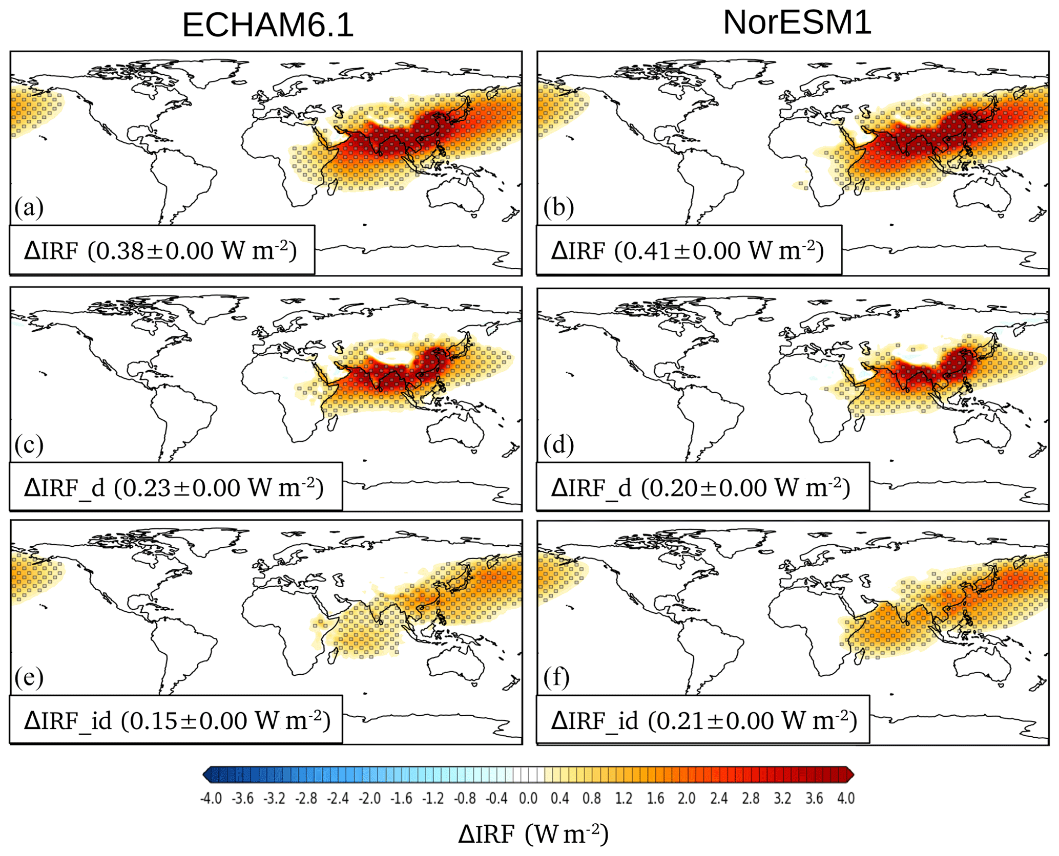
Figure A1The change in the mean instantaneous radiative forcings for runs without and with SE Asian aerosols shown for the individual models (a, c, e, ECHAM6.1; b, d, f, NorESM1).
Table A1Upper rows for each model and model mean: yearly global-mean values in kelvins, with errors on the means given with a 95 % confidence interval. Error on the model mean is given as a pooled sample standard error on the mean. Values in brackets show the standard deviations in yearly mean values (pooled standard deviations for model mean). The bottom row: spatial correlation between NorESM1 and ECHAM6.1.
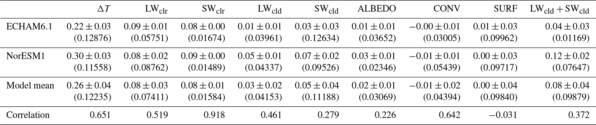
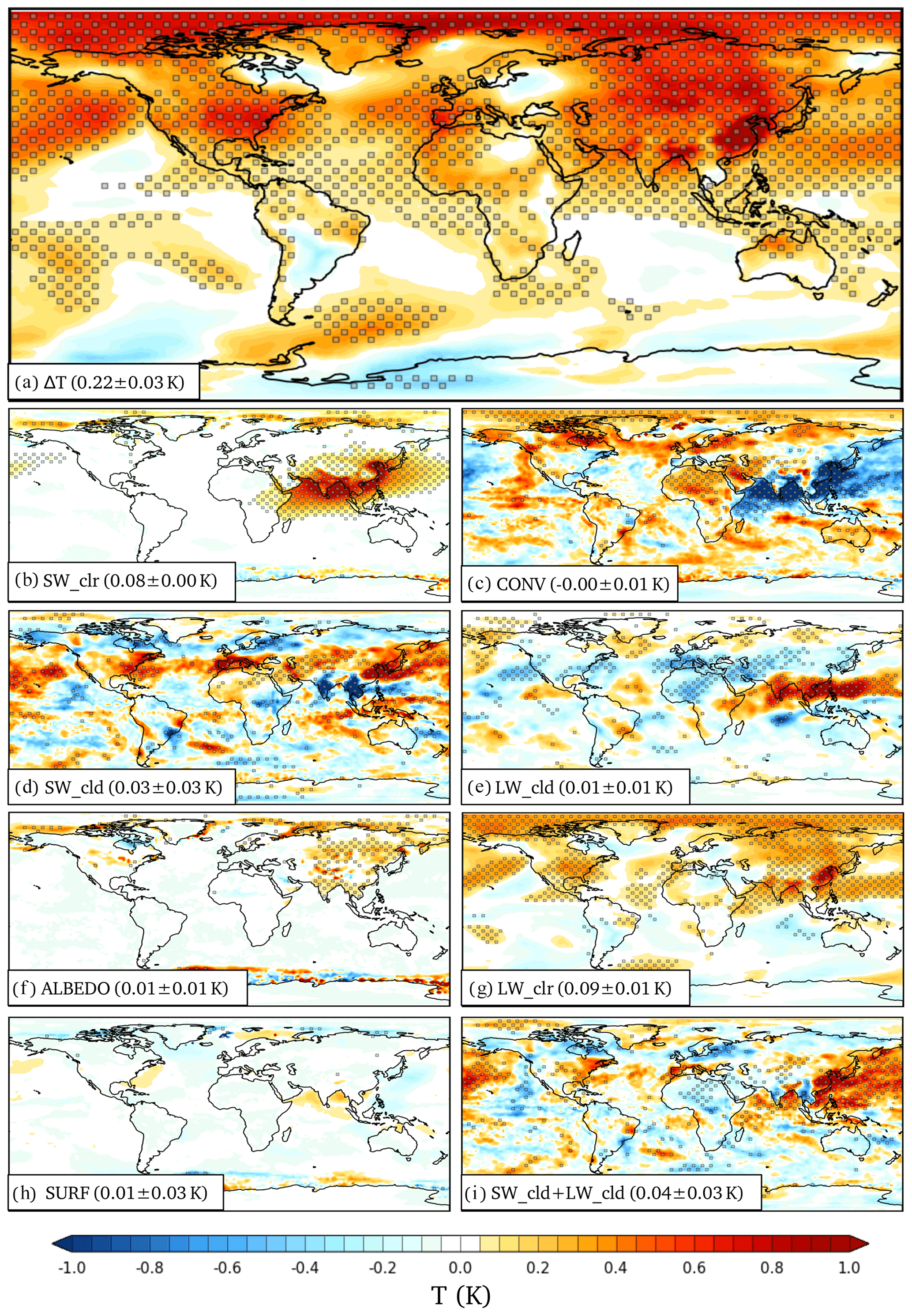
Figure A2The geographical distributions of annually averaged surface air (2 m) temperature responses due to the removal of South and East Asian aerosols for ECHAM6.1. Brackets show global averages. (a) The total surface response. (b–h) Contributions to the total surface temperature response from shortwave clear-sky response (b), horizontal atmospheric heat transport (c), shortwave cloud response (d), longwave cloud response (e), surface albedo change (f), longwave clear-sky response (g), and surface energy flux change (h). (b–h) Sum up to the response seen in panel (a). Panel (i) shows the combined shortwave and longwave cloud response.
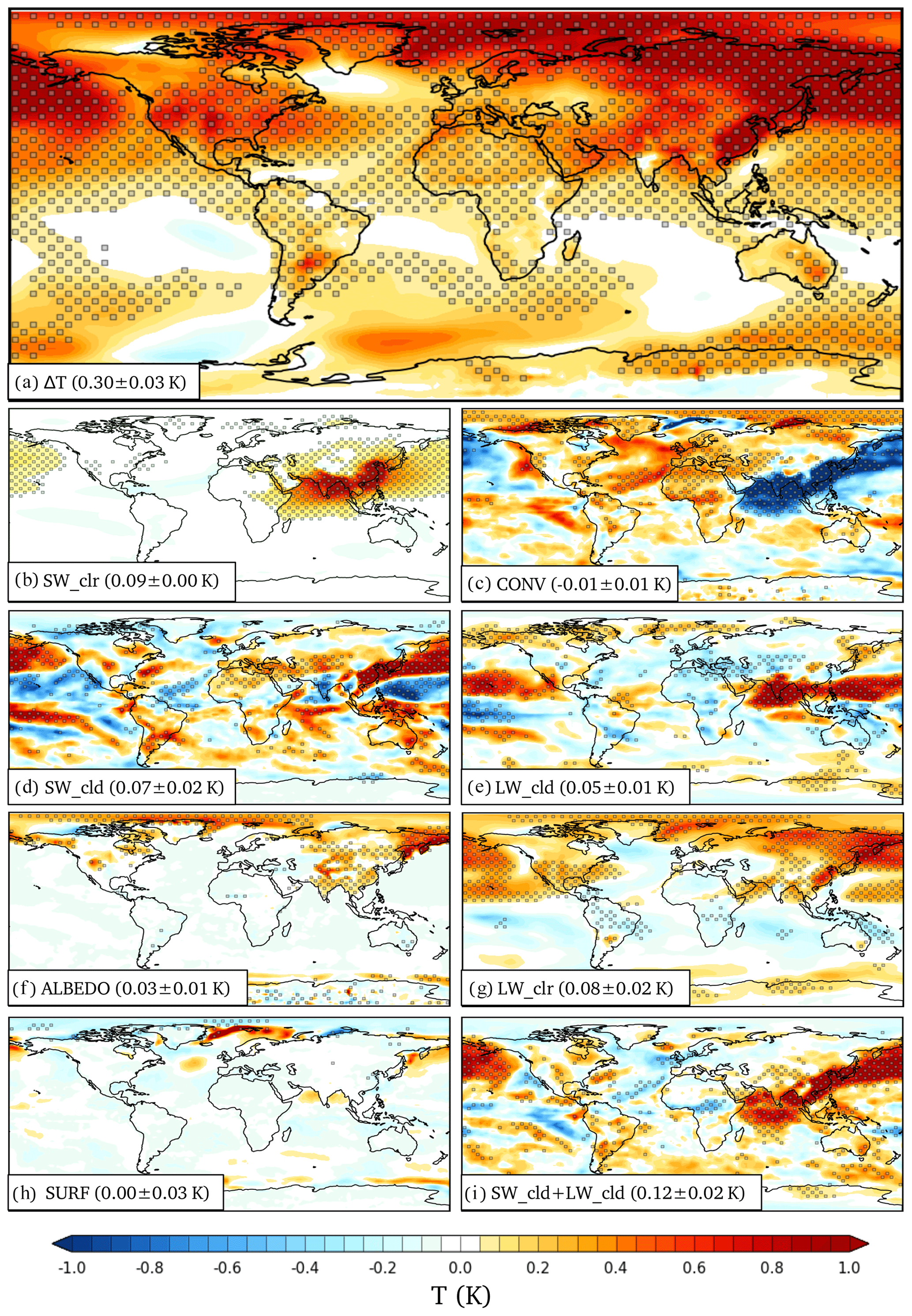
Figure A3As Fig. A2 but for the NorESM1 model.
Data and scripts are available at https://doi.org/10.23728/fmi-b2share.aa3085799bff4be798342e4c0d66caa3 (Merikanto et al., 2020).
The manuscript was written by JM with contributions from all authors. KN performed ECHAM6.1 simulations with help from JM, PR, and DO'D. PR performed all NorESM1 simulations. The data analysis was carried out by JM and KN and guided by JR. HK came up with the initial research idea, and AIP assisted with project coordination.
The authors declare that they have no conflict of interest.
We wish to thank the editor and the two anonymous reviewers for the constructive comments on the manuscript. The authors would also like to thank Stephanie Fiedler for providing the MACv2-SP code for ECHAM6.1.
This research has been supported by the European Research Council (ECLAIR, grant no. 646857) and the Academy of Finland (grant nos. 287440 and 308365).
This paper was edited by Kostas Tsigaridis and reviewed by two anonymous referees.
Acosta Navarro, J. C., Varma, V., Riipinen, I., Seland, Ø., Kirkevåg, A., Struthers, H., Iversen, T., Hansson, H. C., and Ekman, A. M. L.: Amplification of Arctic warming by past air pollution reductions in Europe, Nat. Geosci., 9, 277–281, https://doi.org/10.1038/ngeo2673, 2016.
Apte, J. S., Brauer, M., Cohen, A. J., Ezzati, M., and Pope, C. A.: Ambient PM2.5 reduces global and regional life expectancy, Environ. Sci. Technol. Lett., 5, 546–551, https://doi.org/10.1021/acs.estlett.8b00360, 2018.
Balakrishnan, K., Dey, S., Gupta, T., Dhaliwal, R. S., Brauer, M., Cohen, A. J., Stanaway, J. D., Beig, G., Joshi, T. K., Aggar-wal, A. N., Sabde, Y., Sadhu, H., Frostad, J., Causey, K., God-win, W., Shukla, D. K., Kumar, G. A., Varghese, C. M., Mu-raleedharan, P., Agrawal, A., Anjana, R. M., Bhansali, A., Bhard-waj, D., Burkart, K., Cercy, K., Chakma, J. K., Chowdhury, S., Christopher, D. J., Dutta, E., Furtado, M., Ghosh, S., Ghoshal, A. G., Glenn, S. D., Guleria, R., Gupta, R., Jeemon, P., Kant, R., Kant, S., Kaur, T., Koul, P. A., Krish, V., Krishna, B., Larson, S. L., Madhipatla, K., Mahesh, P. A., Mohan, V., Mukhopad-hyay, S., Mutreja, P., Naik, N., Nair, S., Nguyen, G., Odell, C. M., Pandian, J. D., Prabhakaran, D., Prabhakaran, P., Roy, A., Salvi, S., Sambandam, S., Saraf, D., Sharma, M., Shrivastava, A., Singh, V., Tandon, N., Thomas, N. J., Torre, A., Xavier, D., Yadav, G., Singh, S., Shekhar, C., Vos, T., Dandona, R., Reddy, K. S., Lim, S. S., Murray, C. J. L., Venkatesh, S., and Dan-dona, L.: The impact of air pollution on deaths, disease burden, and life expectancy across the states of India: the Global Bur-den of Disease Study 2017, Lancet Planetary Health, 3, e26–e39, https://doi.org/10.1016/S2542-5196(18)30261-4, 2019.
Bitz, C., Shell, K., Gent, P., Bailey, D., Danabasoglu, G., Armour, K., Holland, M., and Kiehl, J.: Climate Sensitivity of the Com-munity Climate System Model, Version 4, J. Clim., 25, 3053–3070, https://doi.org/10.1175/JCLI-D-11-00290.1, 2012.
Block, K. and Mauritsen, T.: Forcing and feedback in the MPI-ESM-LR coupled model under abruptly quadrupled CO2, J. Adv. Model. Earth Sy., 5, 676–691, 2013.
Carslaw, K., Lee, L., Reddington, C., Pringle, K., Rap, A., Forster, P., Mann, G., Spracklen, D., Woodhouse, M., Regayre, L., and Pierce, J. R.: Large contribution of natural aerosols to uncertainty in indirect forcing, Nature, 503, 67–71, 2013.
Fiedler, S., Kinne, S., Huang, W. T. K., Räisänen, P., O'Donnell, D., Bellouin, N., Stier, P., Merikanto, J., van Noije, T., Makkonen, R., and Lohmann, U.: Anthropogenic aerosol forcing – insights from multiple estimates from aerosol-climate models with reduced complexity, Atmos. Chem. Phys., 19, 6821–6841, https://doi.org/10.5194/acp-19-6821-2019, 2019.
Holland, M. and Bitz, C.: Polar amplification of climate change in coupled models, Clim. Dyn., 21, 221–232, https://doi.org/10.1007/s00382-003-0332-6, 2003.
Iversen, T., Bentsen, M., Bethke, I., Debernard, J. B., Kirkevåg, A., Seland, Ø., Drange, H., Kristjansson, J. E., Medhaug, I., Sand, M., and Seierstad, I. A.: The Norwegian Earth System Model, NorESM1-M – Part 2: Climate response and scenario projections, Geosci. Model Dev., 6, 389–415, https://doi.org/10.5194/gmd-6-389-2013, 2013.
Kasoar, M., Voulgarakis, A., Lamarque, J.-F., Shindell, D. T., Bellouin, N., Collins, W. J., Faluvegi, G., and Tsigaridis, K.: Regional and global temperature response to anthropogenic SO2 emissions from China in three climate models, Atmos. Chem. Phys., 16, 9785–9804, https://doi.org/10.5194/acp-16-9785-2016, 2016.
Kasoar, M., Shawki, D., and Voulgarakis, A.: Similar spatial patterns of global climate response to aerosols from different regions, Clim. Atmos. Sci., 1, 12, https://doi.org/10.1038/s41612-018-0022-z, 2018.
Kinne, S., O'Donnell, D., Stier, P., Kloster, S., Zhang, K., Schmidt, H., Rast, S., Giorgetta, M., Eck, T. F., and Stevens, B.: MAC-v1: A new global aerosol climatology for climate studies, J. Adv. Model. Earth Sy., 5, 704–740, https://doi.org/10.1002/jame.20035, 2013.
Kirkevåg, A., Iversen, T., Seland, Ø., Hoose, C., Kristjánsson, J. E., Struthers, H., Ekman, A. M. L., Ghan, S., Griesfeller, J., Nilsson, E. D., and Schulz, M.: Aerosol–climate interactions in the Norwegian Earth System Model – NorESM1-M, Geosci. Model Dev., 6, 207–244, https://doi.org/10.5194/gmd-6-207-2013, 2013.
Lamarque, J.-F., Bond, T. C., Eyring, V., Granier, C., Heil, A., Klimont, Z., Lee, D., Liousse, C., Mieville, A., Owen, B., Schultz, M. G., Shindell, D., Smith, S. J., Stehfest, E., Van Aardenne, J., Cooper, O. R., Kainuma, M., Mahowald, N., McConnell, J. R., Naik, V., Riahi, K., and van Vuuren, D. P.: Historical (1850–2000) gridded anthropogenic and biomass burning emissions of reactive gases and aerosols: methodology and application, Atmos. Chem. Phys., 10, 7017–7039, https://doi.org/10.5194/acp-10-7017-2010, 2010.
Liu, L., Shawki, D., Voulgarakis, A., Kasoar, M., Samset, B. H., Myhre, G., Forster, P. M., Hodnebrog, Ø., Sillmann, J., Aalbergsjø, S. G., Boucher, O., Faluvegi, G., Iversen, T., Kirkevåg, A., Lamarque, J.-F., Olivié, D., Richardson, T., Shindell, D., Takemura, T., Liu, L., Shawki, D., Voulgarakis, A., Kasoar, M., Samset, B. H., Myhre, G., Forster, P. M., Hodnebrog, Ø., Sillmann, J., Aalbergsjø, S. G., Boucher, O., Faluvegi, G., Iversen, T., Kirkevåg, A., Lamarque, J.-F., Olivié, D., Richardson, T., Shindell, D., and Takemura, T.: A PDRMIP Multimodel Study on the Impacts of Regional Aerosol Forcings on Global and Regional Precipitation, J. Clim., 31, 4429–4447, https://doi.org/10.1175/JCLI-D-17-0439.1, 2018.
Loeb, N. G., Doelling, D. R., Wang, H. L., Su, W. Y., Nguyen, C., Corbett, J. G., Liang, L. S., Mitrescu, C., Rose, F. G., and Kato, S.: Clouds and the Earth's Radiant Energy System (CERES)Energy Balanced and Filled (EBAF) Top-of-Atmosphere (TOA)Edition-4.0 Data Product, J. Clim., 31, 895–918, 2018.
Lund, M. T., Myhre, G., and Samset, B. H.: Anthropogenic aerosol forcing under the Shared Socioeconomic Pathways, Atmos. Chem. Phys., 19, 13827–13839, https://doi.org/10.5194/acp-19-13827-2019, 2019.
Mauritsen, T. and Roeckner, E.: Tuning the MPI-ESM1.2 global climate model to improve the match with instrumental record warming by lowering its climate sensitivity, J. Adv. Model. Earth Sy., 12, e2019MS002037, https://doi.org/10.1029/2019MS002037, 2020.
Merikanto, J., Nordling, K., and Räisänen, P.: How Asian aerosols impact regional surface temperatures across the globe; NorESM1 and ECHAM6.1 data, Finnish Meteorological Institute, https://doi.org/10.23728/fmi-b2share.aa3085799bff4be798342e4c0d66caa3, 2020.
Murphy, D. M.: Little net clear-sky radiative forcing from recent regional redistribution of aerosols, Nat. Geosci., 6, 258–262, 2013.
Myhre, G., Kramer, R. J., Smith, C. J., Hodnebrog, Ø., Forster, P., Soden, B. J., Samset, B. H., Stjern, C. W., Andrews, T., Boucher, O., Faluvegi, G., Fläschner, D., Kasoar, M., Kirkevåg, A., Lamarque, J. F., Olivié, D., Richardson, T., Shindell, D., Stier, P., Takemura, T., Voulgarakis, A., and Watson-Parris, D.: Quantifying the Importance of Rapid Adjustments for Global Precipitation Changes, Geophys. Res. Lett., 45, 11399–11405, https://doi.org/10.1029/2018GL079474, 2018.
NOAA National Centers for Environmental Information, State of the Climate: Global Climate Report for Annual 2019, https://www.ncdc.noaa.gov/sotc/global/201913 (last access: 24 June 2020), 2020.
Nordling, K., Korhonen, H., Räisänen, P., Alper, M. E., Uotila, P., O'Donnell, D., and Merikanto, J.: Role of climate model dynamics in estimated climate responses to anthropogenic aerosols, Atmos. Chem. Phys., 19, 9969–9987, https://doi.org/10.5194/acp-19-9969-2019, 2019.
Persad, G. G. and Caldeira, K.: Divergent global-scale temperature effects from identical aerosols emitted in different regions, Nat. Commun., 9, 3289, https://doi.org/10.1038/s41467-018-05838-6, 2018.
Pithan, F. and Mauritsen, T.: Arctic amplification dominated by temperature feedbacks in contemporary climate models, Nat. Geosci., 7, 181–184, https://doi.org/10.1038/ngeo2071, 2014.
Porter, D. F., Cassano, J. J., Serreze, M. C., and Kindig, D. N.: New estimates of the large-scale Arctic atmospheric energy budget, J. Geophys. Res., 115, D08108, https://doi.org/10.1029/2009JD012653, 2010.
Roeckner, E., Bäuml, G., Bonaventura, L., Brokopf, R., Esch, M., Giorgetta, M., Hagemann, S., Kirchner, I., Kornblueh, L., Manzini, E., Rhodin, A., Schlese, U., Schulzweida, U., and Tompkins, A.: The atmospheric general circulation model ECHAM5. PART I: Model description, Tech. Rep. 349, Max-Planck-Inst. fur Meteorol., Hamburg, Germany, 2003.
Räisänen, J.: An energy balance perspective on regional CO2-induced temperature changes in CMIP5 models, Clim. Dynam., 48, 3441-3454, 2017.
Räisänen, J. and Ylhäisi, J. S.: CO2-induced climate change in northern Europe: CMIP2 versus CMIP3 versus CMIP5, Clim. Dynam., 45, 1877–1897, 2015.
Räisänen, P., Makkonen, R., Kirkevåg, A., and Debernard, J. B.: Effects of snow grain shape on climate simulations: sensitivity tests with the Norwegian Earth System Model, The Cryosphere, 11, 2919–2942, https://doi.org/10.5194/tc-11-2919-2017, 2017.
Samset, B. H., Sand, M., Smith, C. J., Bauer, S. E., Forster, P. M., Fuglestvedt, J. S., Osprey, S., and Schleussner, C.-F.: Climate Impacts From a Removal of Anthropogenic Aerosol Emissions, Geophys. Res. Lett., 45, 1020–1029, https://doi.org/10.1002/2017GL076079, 2018.
Screen, J. A. and Simmonds, I.: The central role of diminishing sea ice in recent Arctic temperature amplification, Nature, 464, 1334–1337, 2010.
Shindell, D., Faluvegi, G., Rotstayn, L., and Milly, G.: Spatial patterns of radiative forcing and surface temperature change, J. Geophys. Res., 120, 5385–5403, https://doi.org/10.1002/2014JD022752, 2015.
Soden, B. J., Broccoli, A. J., and Hemler, R. S.: On the use of cloud forcing to estimate cloud feedback, J. Clim., 17, 3661–3665, 2004.
Stevens, B., Giorgetta, M., Esch, M., Mauritsen, T., Crueger, T., Rast, S., Salzmann, M., Schmidt, H., Bader, J., Block, K., Brokopf, R., Fast, I., Kinne, S., Kornblueh, L., Lohmann, U., Pin-cus, R., Reichler, T., and Roeckner, E.: Atmospheric component of the MPI-M Earth System Model: ECHAM6, J. Adv. Model. Earth Sy., 5, 146–172, 2013.
Stevens, B., Fiedler, S., Kinne, S., Peters, K., Rast, S., Müsse, J., Smith, S. J., and Mauritsen, T.: MACv2-SP: a parameterization of anthropogenic aerosol optical properties and an associated Twomey effect for use in CMIP6, Geosci. Model Dev., 10, 433–452, https://doi.org/10.5194/gmd-10-433-2017, 2017.
Shindell, D. T., Schulz, M., Ming, Y., Takemura, T., Faluvegi, G., and Ramaswamy, V.: Spatial scales of climate response to in-homogeneous radiative forcing, J. Geophys. Res., 115, D19110, https://doi.org/10.1029/2010JD014108, 2010.
Taylor, K. E., Crucifix, M., Braconnot, P., Hewitt, C. D., Doutriaux, C., Broccoli, A. J., Mitchell, J. F. B., and Webb, M. J.: Estimating Shortwave Radiative Forcing and Response in Climate Models, J. Clim., 20, 2530–2543, https://doi.org/10.1175/JCLI4143.1, 2007.
Westervelt, D. M., Mascioli, N. R., Fiore, A. M., Conley, A. J., Lamarque, J.-F., Shindell, D. T., Faluvegi, G., Previdi, M., Correa, G., and Horowitz, L. W.: Local and remote mean and extreme temperature response to regional aerosol emissions reductions, Atmos. Chem. Phys., 20, 3009–3027, https://doi.org/10.5194/acp-20-3009-2020, 2020.
Wilcox, L. J., Liu, Z., Samset, B. H., Hawkins, E., Lund, M. T., Nordling, K., Undorf, S., Bollasina, M., Ekman, A. M. L., Krishnan, S., Merikanto, J., and Turner, A. G.: Accelerated increases in global and Asian summer monsoon precipitation from future aerosol reductions, Atmos. Chem. Phys., 20, 11955–11977, https://doi.org/10.5194/acp-20-11955-2020, 2020
Zwiers, F. W. and von Storch, H.: Taking Serial Correlation into Account in Tests of the Mean, J. Clim., 8, 336–351, 1995.