The impact threshold of the aerosol radiative forcing on the boundary layer structure in the pollution region

Recently, there has been increasing interest in the relation between particulate matter (PM) pollution and atmospheric-boundary-layer (ABL) structure. This study aimed to qualitatively assess the interaction between PM and ABL structure in essence and further quantitatively estimate aerosol radiative forcing (ARF) effects on the ABL structure. Multi-period comparative analysis indicated that the key to determining whether haze outbreak or dissipation occurs is whether the ABL structure satisfies the relevant conditions. However, the ABL structure change was in turn highly related to the PM level and ARF. |SFC−ATM| (SFC and ATM are the ARFs at the surface and interior of the atmospheric column, respectively) is the absolute difference between ground and atmosphere layer ARFs, and the |SFC−ATM| change is linearly related to the PM concentrations. However, the influence of ARF on the boundary layer structure is nonlinear. With increasing |SFC−ATM|, the turbulence kinetic energy (TKE) level exponentially decreased, which was notable in the lower layers or ABL, but disappeared at high altitudes or above the ABL. Moreover, the ARF effects threshold on the ABL structure was determined for the first time, namely once |SFC−ATM| exceeded ∼55 W m⁻², the ABL structure tends to quickly stabilize and thereafter change little with increasing ARF. The threshold of the ARF effects on the boundary layer structure could provide useful information for relevant atmospheric-environment improvement measures and policies, such as formulating phased air pollution control objectives.

1 Introduction

Most urban agglomerations in China, such as the North China Plain (NCP), have suffered from poor air quality due to rapid increase in anthropogenic emissions. Beijing, as the capital city of China and the principal city in the NCP area, has frequently experienced severe and persistent haze events (Li et al., 2020; Wang et al., 2018; Xu et al., 2019; Zhong et al., 2018b). Previous studies have found that the occurrence of PM pollution events in Beijing is not only inseparable from the serious primary emissions and fast formation of secondary aerosols (An et al., 2019; Guo et al., 2014; Li et al., 2017; Wang et al., 2014; Zheng et al., 2015; Wang et al., 2012) but also largely affected by the atmospheric-boundary-layer (ABL) structure, which controls the diffusion, transmission and accumulation of pollutants (Han et al., 2009; Miao et al., 2018; Kotthaus and Grimmond, 2018; Zheng et al., 2017). For instance, the PM concentration has a strong relationship with the ABL height (ABLH), which determines the volume available for pollutant dispersion (Haman et al., 2014; Schaefer et al., 2009; Su et al., 2018; Tang et al., 2016). In most instances, heavy-air-pollution episodes occurred with persistent temperature inversions (Xu et al., 2019; Zhong et al., 2017). Weak or calm winds are essential in the long-term increase in air pollutants (Niu et al., 2010; Yang et al., 2016). Additionally, severe air pollution was reported to be positively related to high atmospheric humidity, one of the manifestations of stagnant ABL conditions (Tie et al., 2017; Petäjä et al., 2016). Moreover, the feedback mechanism between the boundary layer structure and aerosol loading during severe pollution events contributing to the outbreak of haze pollution has been presented in previous studies (Huang et al., 2018; Liu et al., 2018; Petäjä et al., 2016; Zhong et al., 2018b, 2019; Zhao et al., 2019).

However, this topic has yet to be fully understood. More work is needed to systematically study the interaction between ABL structure and PM pollution. Since the surface directly influences the ABL, it is the only atmosphere layer characterized by turbulent activities, while higher atmosphere layers are weakly turbulent because of the strongly stable stratification (Munro, 2005). The ABL acts as a notable turbulence buffer coupling the surface with the free atmosphere, and PM and gas pollutants mainly suspended in the ABL are convectively spread throughout it. The change in boundary layer structure determining the accumulation and diffusion of pollutants in it could be largely linked to the difference in turbulent activity (Garratt, 1992). Moreover, the change in solar radiation reaching the ground drives the diurnal ABL evolution (Andrews, 2000), while the diurnal evolution of the atmospheric thermodynamic status could be greatly affected considering a strong aerosol direct radiation effect, namely strongly scattering radiation and absorbing radiation (Dickerson et al., 1997; Liu et al., 2018; Huang et al., 2018; Stone et al., 2008; Zhong et al., 2018a). As previous studies have reported, aerosol absorption and scattering effects during severe air pollution notably enhance atmospheric stability and suppress the boundary layer development (Barbaro et al., 2014; Ding et al., 2016; Wilcox et al., 2016; Yu et al., 2002), considering that the aerosol radiative forcing (ARF) is a critical parameter to quantify the aerosol direct radiation effect (Gong et al., 2014; Li et al., 2010). The influence degree of ARF on the boundary layer structure is still unclear, and thus quantitatively determining the effects of ARF on the ABL structure is urgently needed.

In this study, we systematically analyzed the way the ABL interacts with PM pollution via contrastive analysis of multiple haze episodes based on not only specific meteorological factors but also turbulent activity profiles and atmospheric-stability indicators. Meanwhile, taking the turbulence kinetic energy (TKE) and ARF as important parameters, we further investigated the influence degree of the aerosol direct radiation effect on the boundary layer structure. Additionally, this paper analyzes the interaction between the ABL structure and air pollution using high-resolution and real-observation datasets, such as temperature and humidity profiles of microwave radiometers, horizontal- and vertical-wind-vector profiles of Doppler wind lidar, ABLH, and aerosol backscattering coefficient profiles of ceilometers. Wind profile lidar and microwave radiometers have the advantage of providing direct and continuous observations of the boundary layer over long periods and can characterize the ABL structure up to 2–3 km (Pichugina et al., 2019; Zhao et al., 2019), compensating for the deficiencies in previous research.

2 Data and methods

Figure S1 in the Supplement shows the observation site of the Tower Branch of the Institute of Atmospheric Physics (IAP), Chinese Academy of Sciences (39^∘58^′ N, 116^∘22^′ E; altitude: 58 m) in Beijing and the sampling instruments in this study. The IAP site is a typical urban Beijing site, and all the sampling instruments are placed at the same location, and simultaneous monitoring is conducted. We conducted a 2-month measurement campaign of the PM concentration and aerosol optical depth (AOD) and obtained vertical profiles of atmospheric parameters such as temperature, humidity, wind vectors, atmospheric stability and turbulent activity to better understand how the boundary layer structure responds to the aerosol direct radiation effect.

The algorithm of SBDART (Santa Barbara DISORT Atmospheric Radiative Transfer) (Levy et al., 2007) is the core model to calculate the aerosol radiative forcing parameters. More information on the input parameters of SBDART are presented in Table S2 in the Supplement. A standard mid-latitude atmosphere is used in SBDART in Beijing. AOD and Ångström exponent (AE) at 550 nm were obtained from a sun photometer. Multiple sets of single-scattering albedo (SSA) and backscattering coefficient were calculated based on Mie theory, and surface albedo and path radiation were read from MODIS (MOD04), which is used to calculate radiative forcing at the top of the atmosphere (TOA). The TOA results were combined with MODIS observations, and the results which have the lowest deviation are defined as the actual parameters of aerosols. This set of parameters would be used to calculate the radiative forcing at the surface, top and interior of the atmospheric column (Gong et al., 2014; Lee et al., 2018; Xin et al., 2016). Hourly radiative forcing parameters, including the ARF at the top, surface (SFC) and interior of the atmospheric column (ATM) at an observation site in Beijing, can be calculated based on this algorithm. More detailed descriptions are provided in our previous work (Gong et al., 2014; Lee et al., 2018; Xin et al., 2016).

Air temperature and relative- and absolute-humidity profiles were retrieved with a microwave radiometer (after this referred to as MWR) (RPG-HATPRO-G5 0030109, Germany). The MWR produces profiles with a resolution ranging from 10–30 m up to 0.5 km, profiles with a resolution ranging from 40–70 m between 0.5 and 2.5 km, and profiles with a resolution ranging from 100–200 m from 2 to 10 km at a temporal resolution of 1 s. More detailed information on the RPG-HATPRO-type instrument can be found at https://www.radiometer-physics.de/ (last access: 4 June 2020).

Vertical-wind-speed and horizontal-wind-vector profiles were obtained by a 3D Doppler wind lidar (Windcube 100s, Leosphere, France). The wind measurement results have a spatial resolution ranging from 1–20 m up to 0.3 km and a spatial resolution of 25 m from 0.3 to 3 km at a temporal resolution of 5 s. More instrument details can be found at https://www.vaisala.com/en/wind-lidars/wind-energy (last access: 21 March 2021).

A ceilometer (CL51, Vaisala, Finland) was adopted to acquire atmospheric-backscattering coefficient (BSC) profiles. The CL51 ceilometer digitally receives the return backscattering signal from 0 to 100 µs and provides BSC profiles with a spatial resolution of 10 m from the ground to a height of 15 km. The ABLH was further identified by the sharp change in the BSC profile's negative gradient (Münkel et al., 2007), and detailed information is reported in previous studies (Tang et al., 2015, 2016; Zhu et al., 2018).

A CIMEL sun photometer (CE318, France), a multichannel, automatic sun-and-sky-scanning radiometer (Gregory, 2011), was used to observe the AOD, and the AOD at 500 nm is adopted in this paper. The real-time hourly mean ground levels of PM_2.5 (particulate matter with aerodynamic diameter less than or equal to 2.5 µm) and PM₁₀ (particulate matter with aerodynamic diameter less than or equal to 10 µm) were downloaded from the China National Environmental Monitoring Center (CNEMC) (available at http://106.37.208.233:20035/, last access: 4 June 2020).

More atmospheric parameters regarding the boundary layer structure used in this study are introduced in Sect. S1 in the Supplement.

3 Results and discussion

3.1 General haze episodes over Beijing in winter

It is well known that severe air pollution episodes frequently occur in Beijing during winter (Li et al., 2007; Zhang et al., 2017). The 2-month PM concentration data from Beijing in the winter of 2018 were collected. As expected, during this time, Beijing experienced severe and frequent haze pollution episodes, with two heavy episodes in which the maximum hourly PM_2.5 concentration reached ∼200 µg m⁻³ and six moderate episodes in which the PM_2.5 mass concentration ranged from ∼100–150 µg m⁻³ (Fig. S2a).

Although the air pollution process is variable and complicated, it is worth stating that Beijing's haze pollution in winter can be generally classified as two kinds of patterns, as shown in Fig. S2b. For all haze episodes ①–⑦, the PM_2.5 mass concentration slowly increased in the afternoon (all times are in local time, or UTC+8) of the first day, followed by a secondary maximum in the early morning and a maximum at midnight of the second day. In comparison to the processes of ④–⑦, where the PM_2.5 mass concentration sharply decreased to <25 µg m⁻³ in the early morning of the third day, during periods ①–③, the highest PM_2.5 mass concentration (∼100–200 µg m⁻³) was observed on the whole third day, which disappeared on the fourth day. As previously reported, transport, chemical transformation and boundary layer structure (local meteorological conditions) are central to determining the amount and type of pollutant loading. Considering the equivalent emission and transport effects, the suspended particles in ④–⑦ subjected to diffuse would be controlled by the atmospheric motion (wind and turbulence) on the third day. The particles during periods ①–③ continuing to accumulate were therefore highly related to the specific ABL status. To investigate the possible reasons for the different variation trends of haze episodes ①–③ and ④–⑦, in the next section, we mainly focus on the ABL structure (local meteorological conditions) influences.

3.2 Qualitative analysis of the interaction between particulate matter and boundary layer structure

The haze episodes in winter in Beijing basically followed two different kinds of variation patterns as described in the previous section. The specific reason for this finding is systematically analyzed in this section. To better illustrate the two different haze patterns, a typical clean period is considered a control. The typical air pollution episodes I (E-I) (13–16 December 2018) and II (E-II) (5–8 January 2019) as well as the typical clean episode III (E-III) (27–30 December 2018) are chosen as examples for analysis.

3.2.1 Similar change trends in the first 2 d

Numerous studies have reported that PM's original explosive growth is caused by pollution transport under southerly winds (Ma et al., 2017; Zhao et al., 2019; Zhong et al., 2018a). In this study, the action of southerly winds on the air pollution in Beijing was presented more clearly as the Windcube 100s lidar obtained the distribution of the horizontal wind vectors extending to heights of 1–1.5 km (equivalent to the entire ABL) (Fig. 1c). On the first day of E-I and E-II, the atmosphere layer up to ∼1 km in height was controlled by strong and clean north winds, exactly like clean E-III. No pollution transport occurred, and the PM and ARF levels were equivalent to those on a clean day (Fig. 1a, b). The atmospheric-backscattering coefficients throughout the ABL during the three episodes only ranged from ∼0–1.5 M m⁻¹ sr⁻¹ (Fig. 3c). From the evening of the first day to the forenoon of the second day, strong southerly winds blew across Beijing during both E-I and E-II, with the wind speed reaching ∼5–15 m s⁻¹ at an atmosphere of about 0.5–1.5 km, while north winds still dominated the ABL during clean E-III. Sensitive to the change in wind direction from north to south, the PM concentration progressively increased from a fairly low level to ∼50 µg m⁻³. Moreover, the BSCs sharply increased to ∼3 Mm⁻¹ rd⁻¹ and were concentrated at altitudes from ∼0.5–1 km, which further stressed the effects of southerly transport on the PM concentration's original growth over Beijing. With prevailing winds originating from the wetter south compared to the low humidity during clean E-III, the air humidity in Beijing during this time also increased, with the vapor density ranging from ∼1.5–2 g m⁻³ for both E-I and E-II (Fig. 3b).

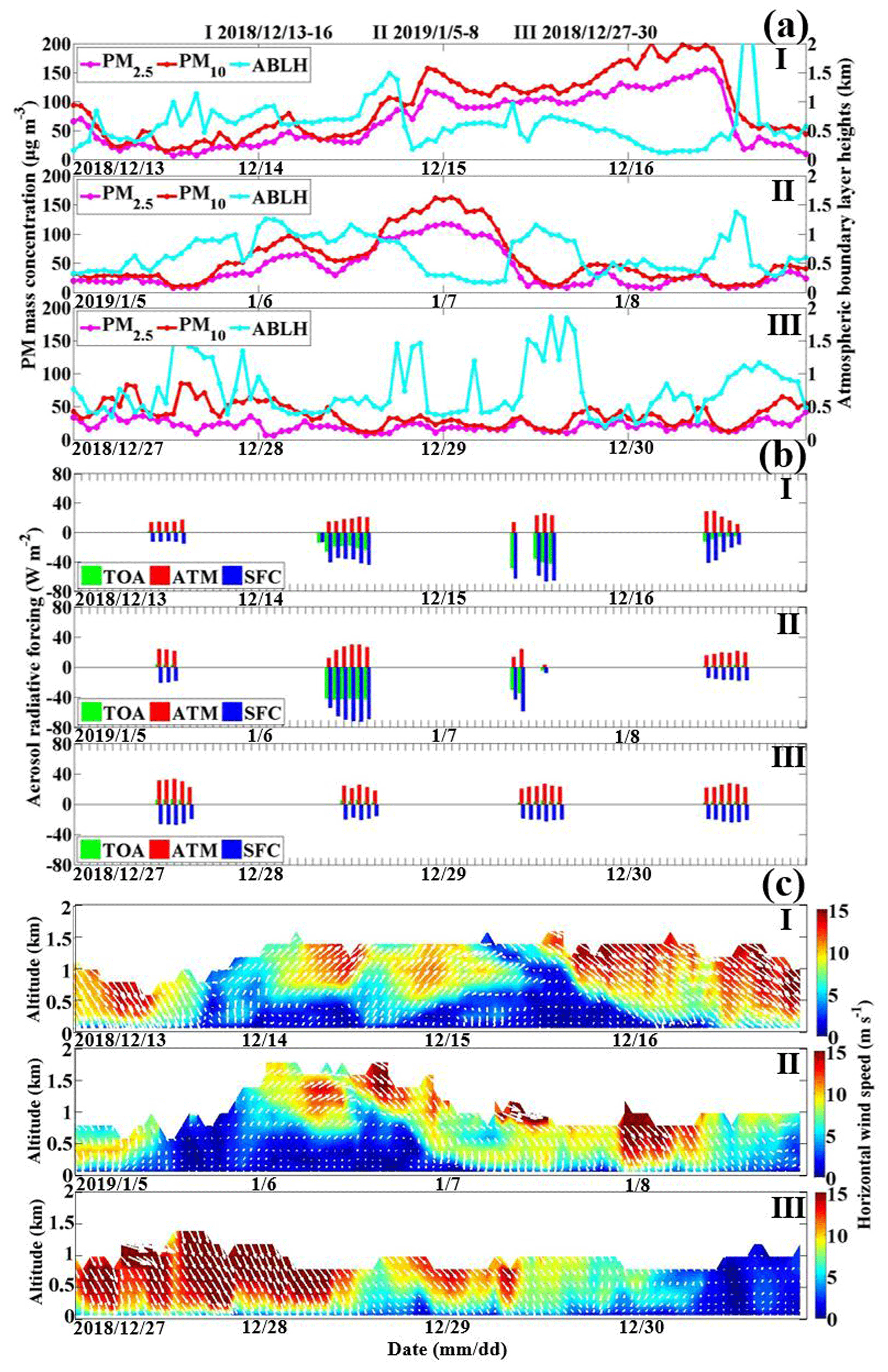
Figure 1 Temporal evolution of (a) the PM mass concentration and atmospheric-boundary-layer height (PM_2.5: solid pink lines; PM₁₀: solid red lines; ABLH: solid blue lines); (b) aerosol radiative forcing at the top (TOA; green bars), surface (SFC; blue bars) and interior of the atmospheric column (ATM; red bars); and (c) horizontal-wind-vector profiles (shaded colors: wind speeds; white arrows: wind vectors) during the typical haze pollution episodes of I (13–16 December 2018) and II (5–8 January 2019) as well as the typical clean period of III (27–30 December 2018).

At midnight of the second day, the PM concentration reached its highest level with a PM_2.5 (PM₁₀) concentration of ∼110 (150) µg m⁻³ during both E-I and E-II. Meanwhile, the highest BSC values mainly occurred from the ground to a height of 1 km at this time, implying that a portion of the suspended particles was pushed down to the near-surface. Before southerly wind transport occurred, the evolution of the stability indicator ($\partial {\mathit{\theta }}_{\mathrm{v}}/\partial z$, $\partial {\mathit{\theta }}_{\mathrm{se}}/\partial z$) profiles during E-I and E-II was analogous to that during clean E-III (Fig. 2a, b). The stratification states at the different heights (0–1 km) were either unstable or neutral, with negative or zero $\partial {\mathit{\theta }}_{\mathrm{v}}/\partial z$ values, respectively, whereby neither clear nor strong temperature inversion phenomena occurred in the boundary layer (Fig. 2c). And the corresponding ABLHs were the same (Fig. 1a). However, the atmospheric stratification from ∼0.5–1 km during E-I and from 0–1 km during E-II became quite stable at night of the second day, with positive values of $\partial {\mathit{\theta }}_{\mathrm{se}}/\partial z$ and weak turbulent activity (TKE: ∼0 m² s⁻²) (Fig. 3a). In contrast to an increased ABLH during clean E-III, the ABLHs during E-I and E-II sharply decreased. Considering strong aerosol scattering and absorbing radiation could affect the temperature stratification (Li et al., 2010; Zhong et al., 2018a). With the elevated PM level due to southerly transport during E-I and E-II, ARF increased as expected, with SFC (ATM) reaching $\sim -\mathrm{40}$ (∼20) and $\sim -\mathrm{75}$ (∼30) W m⁻², respectively. Besides, TOA has an analogous variation trend with SFC, increasing from relatively low values to $\sim -\mathrm{20}$ and $\sim -\mathrm{45}$ W m⁻², respectively. Therefore, less radiation reached the ground, and more heated the atmosphere above the ground during E-I and E-II, and in comparison with clean E-III, the atmospheric stratification was altered, and the stability was thus increased at night. The suspended particles brought by southerly transport originally occurring at high altitudes were restrained from vertically spreading and gradually sank due to gravity and accumulated near the surface.

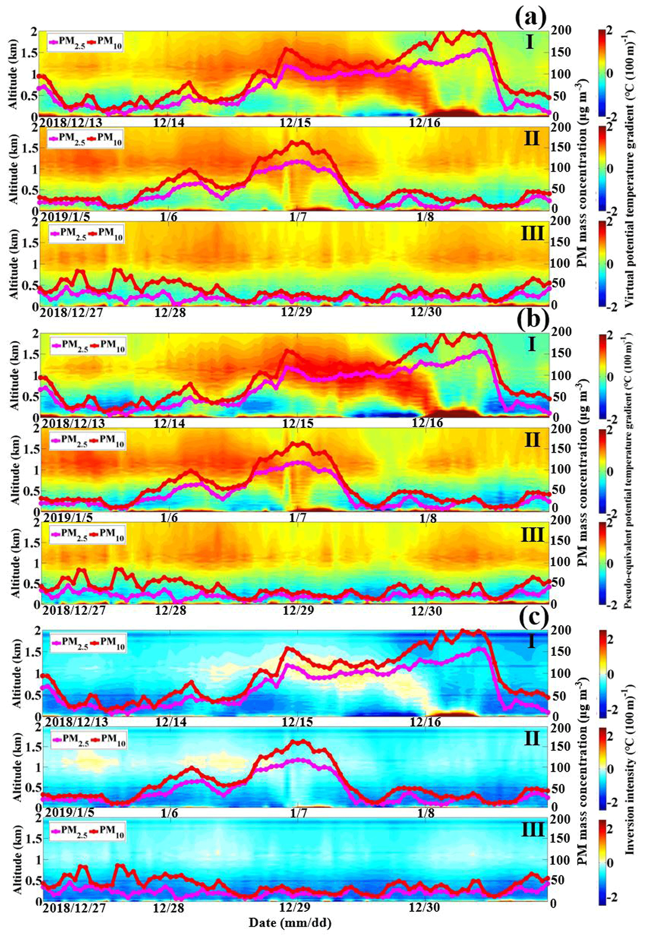
Figure 2 Temporal variation in the vertical profiles of (a) the virtual-potential-temperature gradient ($\partial {\mathit{\theta }}_{\mathrm{v}}/\partial z$), (b) pseudo-equivalent-potential-temperature gradient ($\partial {\mathit{\theta }}_{\mathrm{se}}/\partial z$) and (c) temperature inversion phenomenon (shaded colors: inversion intensity) during the typical haze pollution episodes of I (13–16 December 2018) and II (5–8 January 2019) as well as the typical clean period of III (27–30 December 2018).

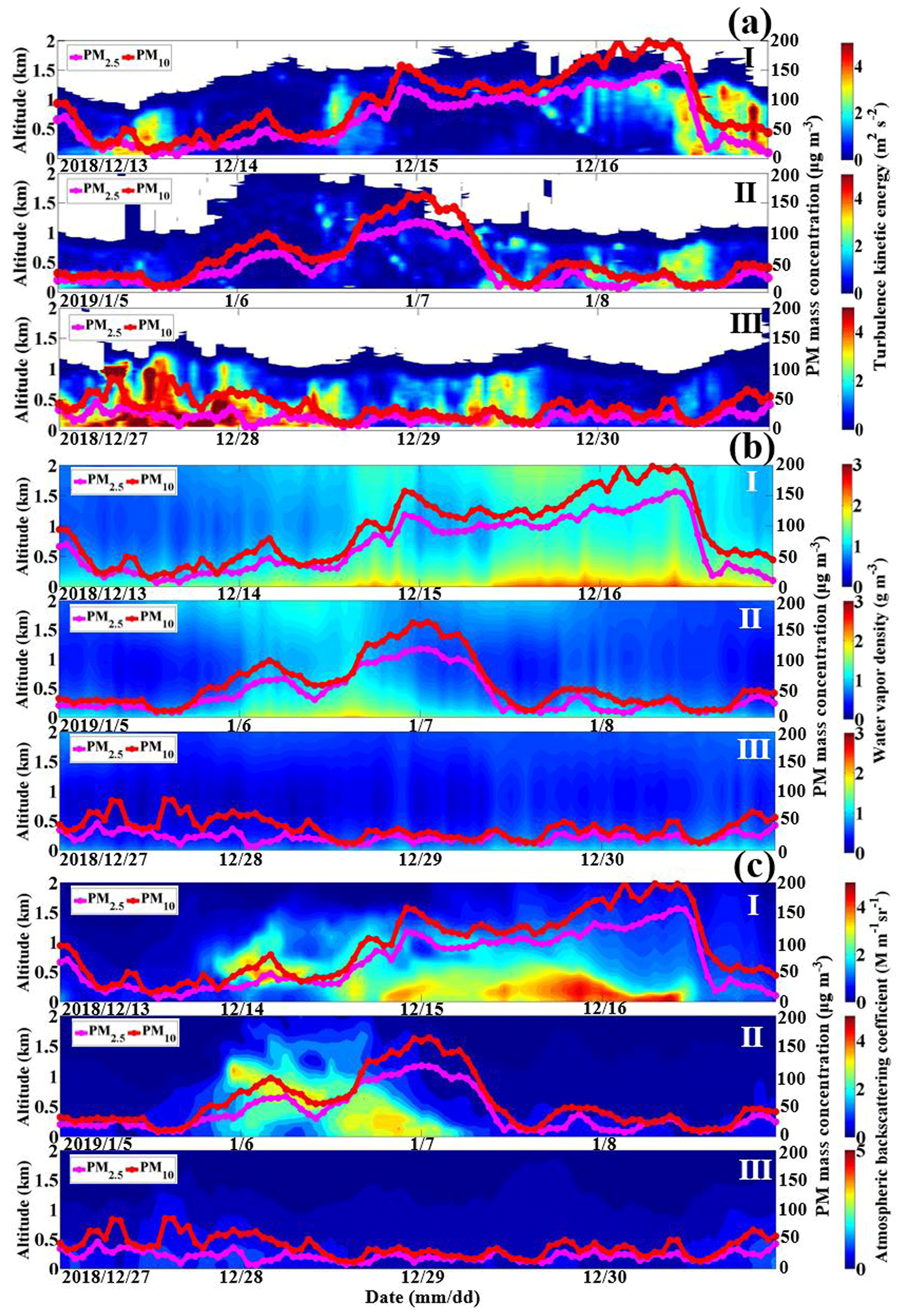
Figure 3 Temporal variation in the vertical profiles of (a) the turbulent activity (shaded colors: TKE), (b) atmospheric humidity (shaded colors: vapor density) and (c) vertical distribution of suspended particles (shaded colors: BSC) during the typical haze pollution episodes of I (13–16 December 2018) and II (5–8 January 2019) as well as the typical clean period of III (27–30 December 2018).

3.2.2 Different change trends in the next 2 d

It is salient to note that the haze evolution trends during E-I and E-II were consistent so far, corresponding to a similar ABL structure. Nevertheless, the north winds (∼10–15 m s⁻¹) during E-II, which only blew above the ABL (>1 km) at midnight of the second day, gradually spread downward and controlled the whole boundary layer on the third day. The wind field is critical concerning horizontal dispersion in the boundary layer; thus, the strong, clean and dry north winds during E-II greatly diffused the already accumulated particles first, where the PM_2.5 mass concentration decreased from ∼100 to ∼50 µg m⁻³. The ARF obtained at 09:00 sharply decreased compared to the previous day, and with solar radiation heating the ground in the morning on the third day, the development of daytime mixing layer eliminated the previous night's temperature structure. The temperature stratification became similar to that on clean E-III, with a similar increase in ABLH. An unstable or neutral atmospheric state with a TKE of ∼2 m² s⁻² was also conducive to the vertical spread of substances. In response, the PM concentration (BSC) and air humidity during E-II gradually decreased with the convective-boundary-layer development and reached the same level as those during clean E-III.

Differently from E-II, in which clean and strong north winds during the third daytime contributed to the diffusion of the previous night's stable stratification, there were still south winds in E-I, which once filled the boundary layer on the second day, gradually decelerating over time from the ground to high altitudes. The atmosphere layer with calm or light winds extended from the ground to a height of ∼1.0 km in the third daytime and gradually down to a height of ∼0.2 km at midnight and the forenoon of the fourth day. Due to the maintained high PM levels, SFC and TOA further increased, up to $\sim -\mathrm{40}$ and $\sim -\mathrm{75}$ W m⁻², respectively, with ATM remaining high (∼25 W m⁻²), which facilitated the temperature inversion that lasted from the whole third day to noon of the fourth day. As shown in Fig. 2a–c-I, there was continued temperature inversion structure from ∼0.5–1.0 km altitude, and the atmospheric stratification was quite stable during the third daytime and at midnight. Since the temperature inversion layer acted as a lid at altitudes of ∼0.5–1.0 km, downward momentum transport would be blocked. Original south winds near the ground were constantly consumed by friction, further explaining the lower atmosphere layer's calm or light winds. With quite strong north winds starting to blow at high altitude during the third night and surface cooling strengthening, the temperature inversion at ∼0.5–1.0 km was gradually broken and turned to ground-touching temperature inversion at 0–0.2 km altitude at midnight. This abnormal temperature structure lasted till noon of the fourth day, mainly due to the strong aerosol direct radiation effect of the pre-existing high PM level. As expected, we can see the strong north winds above ∼1.0 km during the third night gradually extended downward and eventually occurred above the ground-touching inversion in the forenoon of the fourth day. Therefore, with calm or light winds and weak turbulent activity below the temperature inversion on the third day, the PM concentrated exactly below the inversion lid (below ∼0.5 km) and maintained high concentrations, as the BSC distribution shows in Fig. 3c-I. With strong ground-touching inversion of 0–0.2 km altitude forming at midnight and the forenoon of the fourth day, the accumulated particles near the surface were further inhibited right in the stable atmosphere layer (below ∼0.2 km). The same effect was exerted on the water vapor, resulting in the high air humidity below the inversion lid at this time. Therefore, the pollutant layer was compressed downward and accompanied by intense heterogeneous-hydrolysis reactions at the moist particle surface (Zhang et al., 2008), thus resulting in the continued increase in near-surface PM_2.5 concentrations. At noon of the fourth day, the north winds further accelerated with wind speed higher than ∼15 m s⁻¹ and spread down to the whole ABL, which promoted the horizontal and convective dispersion of pollutants and water vapor, and the PM mass concentration, therefore, dropped to the same level as that on clean E-III. With PM_2.5 sharply dropping from ∼150 to ∼20 µg m⁻³ in 4 h, the aerosol direct radiation effect was sensitive to PM changes and gradually decreased from 10:00 to 14:00, finally reaching the same level as those on clean E-III.

In this section, through a detailed contrastive analysis, we examine the potential reasons for the occurrence of the two different patterns of haze pollution in winter in Beijing. We found that the crucial point in determining whether the PM mass concentration remained high or sharply decreased was related to whether the boundary layer remained stable. The boundary layer stability was, in turn, notably linked to the PM mass concentration and aerosol direct radiation effect.

3.3 Quantitative analysis of the effect of particulate matter on the boundary layer structure

Based on the contrastive analysis in the previous section, it was clear that the ABL structure played a critical role in the maintenance and dissipation of air pollution. It appeared that the increase in atmospheric stability suppressed pollution diffusion under a weak turbulence activity and low ABLH. Water vapor also significantly accumulated to a relatively high level near the surface, further facilitating secondary aerosols' formation. The evolution of ABL stability essentially occurred in response to the atmospheric temperature structure, as analyzed above, which was influenced by the strong aerosol direct radiation effect (Andrews, 2000; Li et al., 2010). The Archimedes buoyancy generated by the pulsating temperature field in the gravity field exerted negative work on the turbulent pulsating field, with a stable ABL occurring. The turbulence served as a carrier for the transport of substances like water vapor, heat and PM in the boundary layer (Garratt, 1992). Thus, in the following section, the ARF and TKE are chosen as the key parameters to examine how PM affects and modifies the boundary layer structure.

Figure 4 Scatterplots of the PM_2.5 mass concentration (x) versus aerosol radiative forcing at the top of the atmospheric column (TOA; y; a); the interior of the atmospheric column (ATM; y; b); and the surface (SFC; y; c) as well as the absolute difference in SFC and ATM (|SFC−ATM|; y; d), respectively (gray dots: daily data; other dots: mean data). (The daily data mean daily mean values of TOA, ATM, SFC and corresponding daily averaged PM_2.5 mass concentration from 27 November 2018 to 25 January 2019 in Beijing. The mean PM_2.5 concentrations were obtained by averaging daily PM_2.5 concentrations at intervals of 10 µg m⁻³. The mean TOA, ATM and SFC were obtained after the corresponding daily TOA, ATM and SFC average, respectively. For example, all daily PM_2.5 concentrations greater than 40 µg m⁻³ and less than 50 µg m⁻³ were averaged as a mean PM_2.5 concentration, and TOA values (ATM, SFC) corresponding to this daily PM_2.5 concentration range were also averaged as a mean TOA (ATM, SFC)).

Figure 5 Three-dimensional plot of the fitting relationship of the absolute difference in aerosol radiative forcing between the surface and interior of the atmospheric column (|SFC−ATM|; x) and turbulence kinetic energy (TKE; z) at the different altitudes (y) (a and b present different perspectives).

Figure 4 shows the relationship between the PM concentration and ARF. As shown in Fig. 4a and c, TOA and SFC were proportional to the PM_2.5 concentration, respectively. With the increase in PM_2.5 concentration, elevated aerosol loading near the surface would scatter more solar radiation back into outer space and result in less solar radiation reaching the ground, corresponding to a cooling of the surface and making negative SFC. TOA means the aerosol radiative forcing at the top of the atmosphere column and is the sum of ATM and SFC. Considering that anthropogenic aerosols are mostly scattering aerosols, the SFC forcing is generally stronger than ATM, corresponding to a cooling of the earth–atmosphere system. The TOA forcing was thus usually negative and had a similar trend to SFC. ATM, driven by the aerosol absorption effect and representing a warming effect of aerosols on the atmosphere layer, exhibited a positive correlation with the PM_2.5 concentration (see Fig. 4b). These results demonstrated that a higher PM_2.5 concentration would arouse a stronger ARF, further inhibiting solar radiation from reaching the ground and heating the atmosphere layer more. |SFC−ATM|, defined as the absolute value of the difference between SFC and ATM, represents aerosols' combined action on the solar radiation reaching the aerosol layer and the ground. Larger values of |SFC−ATM| indicate stronger aerosol scattering and/or absorption effects, further implying a more significant temperature difference between the ground and the atmosphere layer above. As expected, a positive linear correlation between |SFC−ATM| and PM_2.5 concentration was found, as shown in Fig. 4d.

As described in the above paragraph, there was a strong ARF under a high PM loading, which markedly altered the atmospheric temperature structure, further changing the ABL structure. It is necessary to determine the effect degree of ARF on the boundary layer structure. Figure 5 shows the 3D plots of the fitting relationship between the hourly values of |SFC−ATM| and TKE at the different altitudes. What stands out in Fig. 5a is the general decline in TKE concerning the growth of |SFC−ATM|. With increasing |SFC−ATM| value, the TKE value at the different altitudes always decreased exponentially and approached 0 below ∼0.8 km. The notable exponential function between TKE and |SFC−ATM| explained that a strong ARF would drastically change the boundary layer into highly stable conditions characterized by a rather low TKE. The results above highlight the aerosol direct radiation effect's non-negligible impact on the boundary layer structure, especially during the haze episode under a high aerosol loading with a strong ARF. It is well known that a larger net negative (positive) SFC (ATM) arouses a cooler (warmer) ground (atmosphere). An increase in |SFC−ATM| implies the gradual intensification of the ground cooling and/or atmosphere heating processes. Therefore, it changed the atmospheric stratification into a gradually enhanced stable state, which was characterized by increasingly weaker turbulence activities. Additionally, as shown in Fig. 5b, we can identify a critical point of the |SFC−ATM| effects on TKE in the low layers. In particular, TKE decreased with increasing |SFC−ATM| and hardly changed when |SFC−ATM| exceeded the critical point.

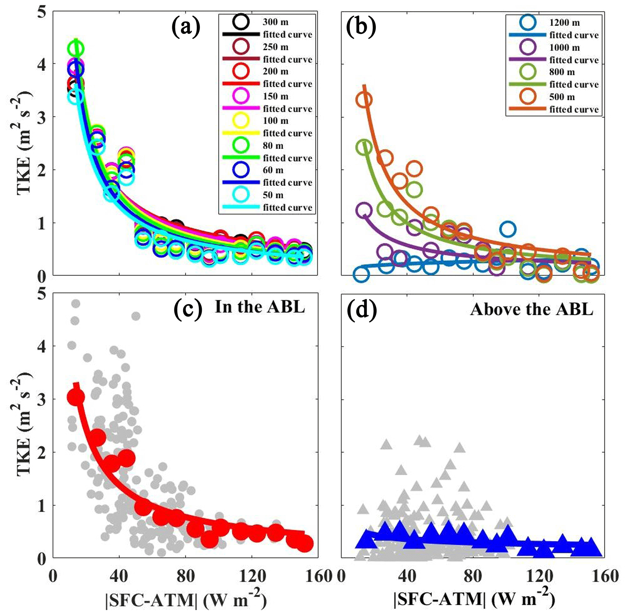
Figure 6 Scatterplots of the mean absolute difference in the aerosol radiative forcing at the surface and interior of the atmospheric column (|SFC−ATM|; x) versus the mean turbulence kinetic energy (TKE; y) at the different altitudes (a, b). Scatterplots of |SFC−ATM| (x) versus TKE (y) in the ABL (c) and above the ABL (d) (gray dots: hourly data; other dots: mean data). The hourly data were collected over a 2-month period in Beijing from 27 November 2018 to 25 January 2019. (The hourly data mean hourly mean values of |SFC−ATM| and corresponding hourly TKE. The mean |SFC−ATM| was obtained by averaging hourly |SFC−ATM| at intervals of 10 W m⁻², then the mean TKE was obtained after the average of the corresponding hourly TKE.)

To define the critical point, we generated scatterplots of the average |SFC−ATM| and TKE at different altitudes, as shown in Fig. 6a, b. The scatterplots of the unaveraged hourly data are shown in Fig. S3, and the fitting functions are listed in Table S1. Depending on the exponential curve's maximum curvature (Thompson and Gardner, 1998), a critical point should exist. With the mean TKE and |SFC−ATM| values on the exponential curve, we found that once the aerosol direct radiation effect defined by |SFC−ATM| exceeded 50–60 W m⁻² (average of ∼55 W m⁻²), the TKE sharply decreased from ∼2 m² s⁻² to lower than 1 m² s⁻². This means that a high aerosol loading, with a |SFC−ATM| value higher than ∼55 W m⁻², tends to change the boundary layer from an unstable state to an extremely stable state in a short time, and further increasing |SFC−ATM| would barely modify the ABL structure. The average |SFC−ATM| value of ∼55 W m⁻² can be defined as the threshold of the ARF effects on the ABL structure, which could provide useful information for relevant model simulations, atmospheric-environment improvement measures and relevant policies. Besides, as shown in Figs. 5 and 6, the exponential relationship between TKE and |SFC−ATM| was notable in the low layers and gradually deteriorated with increasing altitude. On average, the exponential relationship was notable in the ABL and almost disappeared above the ABL (Fig. 6c, d). Aerosols are mainly concentrated below the lower atmosphere, contributing the most to the SFC and ATM forcing, which further confirms that the considerable change in atmospheric stratification caused by aerosols existed and mainly occurred in the lower layers.

The previous discussion shows that a strong aerosol direct radiation effect markedly affected the turbulent activity and modified the boundary layer structure. As many studies have reported, the ABLH is an important meteorological factor that influences the vertical diffusion of atmospheric pollutants and water vapor (Stull, 1988; Aron, 1983). The following examines the relationship among the turbulent activity, ARF and ABLH to illustrate the change in ABLH in response to ARF. Figure 7 shows the ABLH as a function of the TKE and |SFC−ATM| at the different altitudes. It was apparent that a positive correlation exists between TKE and ABLH. As the turbulent activity became increasingly weaker, the corresponding boundary layer height gradually decreased, responding to the gradual increase in |SFC−ATM|. Similarly to the relationship between the turbulent activity and aerosol radiative effect, as shown in Fig. 6, the relationship among these aspects was much stronger below 300 m and almost disappeared above 800 m. This further addressed the fact that the change in boundary layer height was attributed to the turbulence activity variation stemming from the aerosol direct radiation effect.

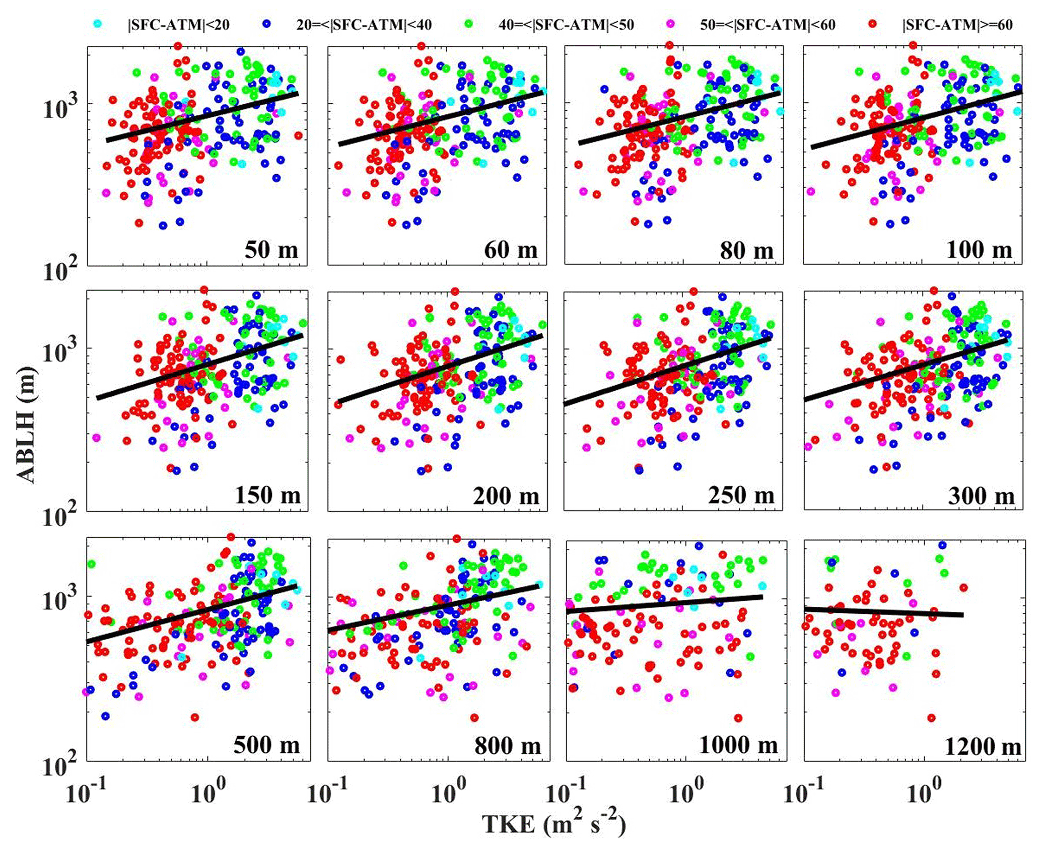
Figure 7 The atmospheric-boundary-layer height (ABLH; y) as a function of the turbulence kinetic energy (TKE; x) at the different altitudes and the aerosol direct radiation effect defined as |SFC−ATM| (color code). The calculated hourly data used above are collected over 2 months in Beijing from 27 November 2018 to 25 January 2019.

This section demonstrates that the aerosol loading with aerosol radiative effects impacted the turbulent activity, changed the boundary layer height and modified the boundary layer structure. On the other hand, it is now necessary to explain how the renewed boundary layer structure modifies the PM_2.5 concentration. As shown in Fig. S4a, b, the ABLH as an independent variable impacts the ambient water vapor in the ABL to some degree. There was a steady increase in the ambient humidity with decreasing ABLH, where absolute humidity (AH) and relative humidity (RH) were projected to decrease to ∼3 g m⁻³ and ∼60 %, respectively, with the ABLH decreasing below ∼500 m. With the increase in ambient humidity, a marked rise in PM_2.5 concentration occurred, as shown in Fig. S4c and d. Once AH and RH exceeded ∼3 g m⁻³ and ∼60 %, respectively, the PM_2.5 concentration reached ∼100 µg m⁻³. The results above indicate that with a fairly low boundary layer height, water vapor accumulated near the surface, and particles tended to hygroscopically grow, resulting in secondary-aerosol formation in a high-humidity environment, further increasing the PM_2.5 concentration. As shown in Fig. S4e, with the level off of the ABLH, the PM_2.5 mass concentration increased exponentially and reached a high value. The exponential relationship was similar to that between the ambient humidity and ABLH, which revealed that the explosive growth of the PM_2.5 concentration under a low ABLH was largely driven by intense secondary-aerosol formation and hygroscopic growth at high ambient humidity.

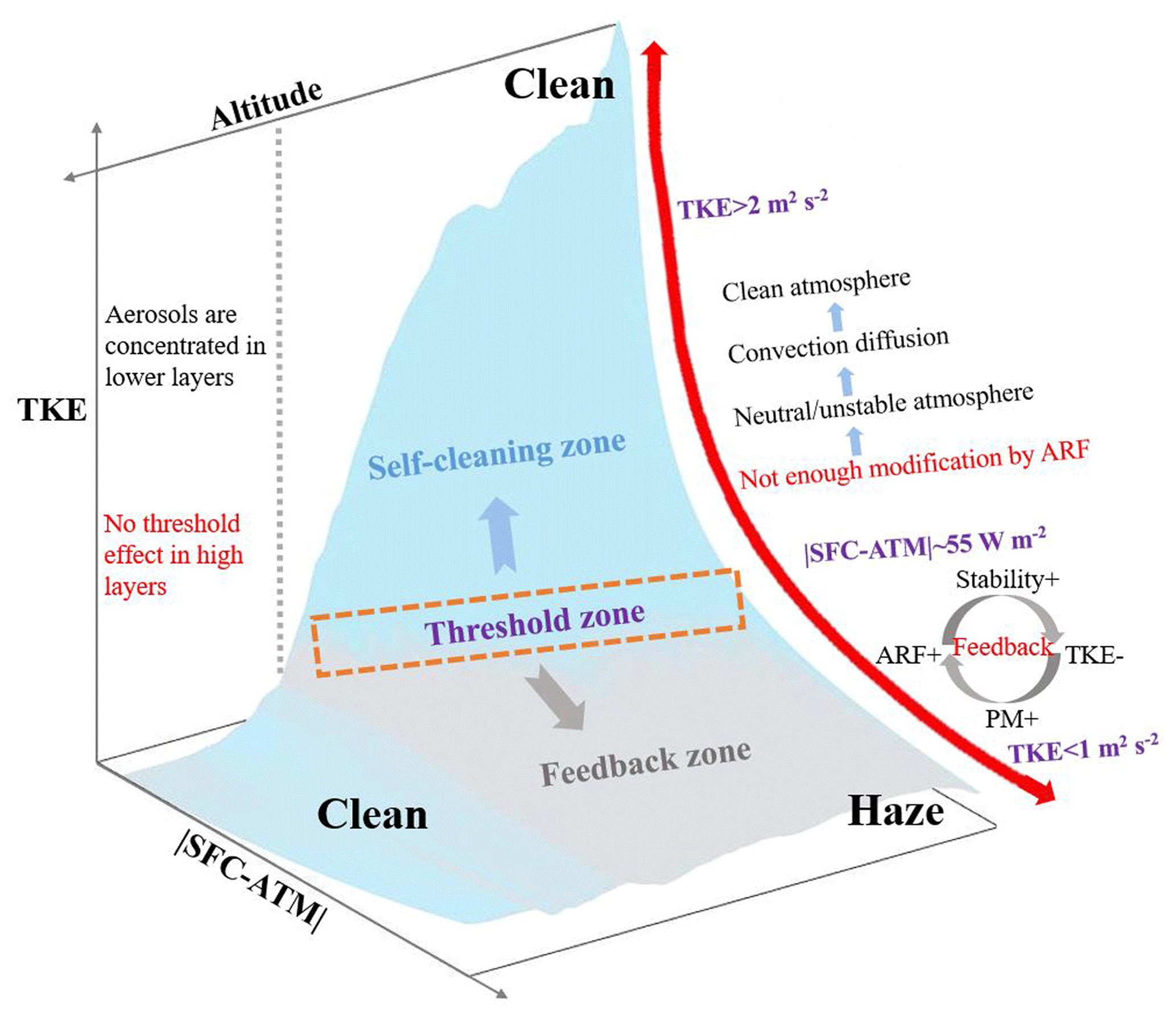
Figure 8 Schematic diagram of the interaction between the aerosol radiative forcing (ARF) and boundary layer structure (|SFC−ATM|: the mean absolute difference in the aerosol radiative forcing at the surface and interior of the atmospheric column; TKE: the mean turbulence kinetic energy).

4 Conclusion

By analyzing the 2-month haze conditions in winter in Beijing, we found that haze pollution basically underwent two different variation patterns, namely the same trends on the first 2 d, and on the next days, one haze pattern went through a continuing outbreak, while the other haze pattern exhibited notable diffusion. Considering equivalent emissions, this has raised important questions about whether and how the local boundary layer structure impacted or caused this difference. The results of a contrastive analysis qualitatively showed that the crucial point in determining whether the PM concentration remained very high or sharply decreased was largely related to whether the boundary layer structure (i.e., stability and TKE) satisfied relevant conditions. As previous studies reported (Liu et al., 2018; Zhong et al., 2018b, 2019) and is confirmed in this paper, the extremely stable stratification with positive $\partial {\mathit{\theta }}_{\mathrm{se}}/\partial z$ values and a low TKE, was the premise of the outbreak of haze pollution. However, the change or state of the boundary layer structure was, in turn, strongly linked to the PM mass concentration and ARF, and we further quantitatively evaluated the effect of ARF on the boundary layer structure. Figure 8, emerging from the previous observation analysis, is where ARF modifies the boundary layer structure and aggravates haze pollution. The ARF effects on the atmospheric stratification depend on the reduced radiation reaching the ground due to aerosol scattering and absorbing radiation in the atmosphere (Dickerson et al., 1997; Stone et al., 2008). Firstly, we found that a positive linear relationship between |SFC−ATM| and PM_2.5 concentration existed, which means the strong aerosol scattering and/or absorption effect occurs during the heavy haze episodes and could arouse significant temperature differences between the surface and the above atmosphere layer. Secondly, previous studies revealed that black carbon solar absorption suppresses turbulence near the surface (Wilcox et al., 2016), while we found that the TKE value at the different altitudes always decreased exponentially with increasing |SFC−ATM|, which was significant in the lower atmosphere layer. Moreover, the ARF effects on turbulent activity were found to be significant in the boundary layer and disappeared above the boundary layer, which also confirmed that the stronger ARF from the aerosol layer would indeed change the boundary layer into the considerably stable state characterized by a relatively low TKE. Thirdly, the ARF change is linear due to the PM concentration; however, the influence of ARF on the boundary layer structure is nonlinear. Based on the exponential relationship, the threshold of the ARF effects on the boundary layer structure has been determined for the first time, highlighting that once the ARF exceeds a specific value, the boundary layer structure tends to quickly stabilize, after that changing little with increasing ARF. This threshold could provide useful information for relevant atmospheric-environment improvement measures and policies in Beijing. When the PM_2.5 concentration is controlled with the ARF below the threshold, the unstable atmosphere's self-purification capacity could effectively dilute and diffuse pollutants. In contrast, when the PM_2.5 concentration increases with an ARF exceeding the threshold value, the boundary layer would stabilize sharply, especially in the lower layers, aggravating haze pollution.