the Creative Commons Attribution 4.0 License.
the Creative Commons Attribution 4.0 License.
 | 01 Apr 2021
Mixing at the extratropical tropopause as characterized by collocated airborne H2O and O3 lidar observations
Andreas Schäfler
Andreas Fix
Martin Wirth
The composition of the extratropical transition layer (ExTL), which is the transition zone between the stratosphere and the troposphere in the midlatitudes, largely depends on dynamical processes fostering the exchange of air masses. The Wave-driven ISentropic Exchange (WISE) field campaign in 2017 aimed for a better characterization of the ExTL in relation to the dynamic situation. This study investigates the potential of the first-ever collocated airborne lidar observations of ozone (O3) and water vapor (H2O) across the tropopause to depict the complex trace gas distributions and mixing in the ExTL. A case study of a perpendicular jet stream crossing with a coinciding strongly sloping tropopause is presented that was observed during a research flight over the North Atlantic on 1 October 2017.
The collocated and range-resolved lidar data that are applied to established tracer–tracer (T–T) space diagnostics prove to be suitable to identify the ExTL and to reveal distinct mixing regimes that enabled a subdivision of mixed and tropospheric air. A back projection of this information to geometrical space shows remarkably coherent structures of these air mass classes along the cross section. This represents the first almost complete observation-based two-dimensional (2D) illustration of the shape and composition of the ExTL and a confirmation of established conceptual models. The trace gas distributions that represent typical H2O and O3 values for the season reveal tropospheric transport pathways from the tropics and extratropics that have influenced the ExTL. Although the combined view of T–T and geometrical space does not inform about the process, location and time of the mixing event, it gives insight into the formation and interpretation of mixing lines. A mixing factor diagnostic and a consideration of data subsets show that recent quasi-instantaneous isentropic mixing processes impacted the ExTL above and below the jet stream which is a confirmation of the well-established concept of turbulence-induced mixing in strong wind shear regions. At the level of maximum winds reduced mixing is reflected in jumps in T–T space that occurred over small horizontal distances along the cross section. For a better understanding of the dynamical and chemical discontinuities at the tropopause, the lidar data are illustrated in isentropic coordinates. The strongest gradients of H2O and O3 are found to be better represented by a potential vorticity-gradient-based tropopause compared to traditional dynamical tropopause definitions using constant potential vorticity values. The presented 2D lidar data are considered to be of relevance for the investigation of further meteorological situations leading to mixing across the tropopause and for future validation of chemistry and numerical weather prediction models.
- Article
(7773 KB) - Full-text XML
- Companion paper
- BibTeX
- EndNote


The extratropical transition layer (ExTL) is a subregion of the extratropical upper troposphere and lower stratosphere (ExUTLS) which is relevant both for climate (Riese et al., 2012) and weather (Gray et al., 2014). Radiatively active trace gases, like ozone (O3) and water vapor (H2O), provide significant vertical gradients across the ExTL, and the tropopause therein, that impact the Earth's radiation budget. The transition from the troposphere to the stratosphere can be abrupt or more uniform in cases when the ExTL is strongly impacted by two-way stratosphere–troposphere exchange (STE) processes. Depending on their lifetime, trace gases reveal a footprint of the mixing processes in their Lagrangian history, typically as an intermediate chemical characteristic with both tropospheric and stratospheric influence, highlighting irreversible and bidirectional transport between the spheres (Gettelman et al., 2011). These mixing processes strongly depend on the dynamical situation. For a better understanding of the role of multiscale dynamical processes on the composition of the ExTL in the midlatitudes, the Wave-driven ISentropic Exchange (WISE) field campaign (Kunkel et al., 2019) was conducted over the North Atlantic Ocean in autumn 2017. The HALO (High Altitude LOng range) research aircraft performed in situ and remote sensing measurements of various trace gases in the ExTL from turbulence to synoptic scales in a variety of meteorological situations.
Mixing in the extratropics is often related to upper-level frontal zone–jet-stream systems (Keyser and Shapiro, 1986; Lang and Martin, 2012) that are characterized by isentropic surfaces that cross the sloped tropopause (Holton et al., 1995; Stohl et al., 2003). The highly variable midlatitude flow is largely affected by baroclinic cyclones that develop from disturbances in the jet stream and cause a strong distortion of the tropopause through the redistribution of tropospheric and stratospheric air masses. Intrusions of stratospheric air into the troposphere are connected to jet streams and cyclones and represent areas of irreversible mixing of tropospheric and stratospheric air due to filamentation (Danielsen, 1968; Danielsen et al., 1987) and roll-up of intrusions (Appenzeller et al., 1996). Strong wind shear above and below the jet stream maximum results in clear air turbulence fostering the exchange between stratosphere and troposphere (Shapiro, 1976, 1980). Recently, Spreitzer et al. (2019) have shown the importance of turbulence in upper-level frontal zone–jet-stream systems and tropopause folds for midlatitude dynamics. Beside turbulence, a variety of other non-conservative diabatic processes occur near jet streams and cyclones that foster cross-isentropic mixing, e.g., cloud diabatic processes in convective or large-scale clouds (Gray, 2003; Wernli and Bourqui, 2000) or radiative processes related to vertical H2O gradients or clouds (Zierl and Wirth, 1997). Additionally, thunderstorms were shown to impact the ExTL composition (e.g., Huntrieser et al., 2016; Pan et al., 2014a), often being triggered by large-scale weather systems. The spatiotemporal diversity of the flow and the complex life of cyclones result in a large variety of mixing and exchange processes that were found through case studies and climatologies (Sprenger and Wernli, 2003; Škerlak et al., 2014; Reutter et al., 2015; Boothe and Homeyer, 2017) and explain the complexity that ExTL observations have shown in terms of their chemical characteristics.
Mixed air masses can be identified by relationships between long-lived chemical trace gases (Hintsa et al., 1998, Fischer et al., 2000; Hoor et al., 2002; Zahn and Brenninkmeijer, 2003; Pan et al., 2004). This correlation of tropospheric and stratospheric tracers with opposing behavior (tracer–tracer or T–T correlation, explained in more detail in Sect. 2.2), e.g., of O3 and H2O, was used to separate mixed air masses of intermediate chemical characteristics from the undisturbed background to explore the average composition and extent of the ExTL (see summary in Gettelman et al., 2011). Many of these climatological studies made use of data from multiple research flights or multiple campaigns or used satellite data. In situ observations of chemical species on board commercial aircraft (e.g., Brenninkmeijer et al., 2007) are restricted to the flight routes and the altitude range of the aircraft and provide only a limited number of vertical profiles during start and landing (Zahn et al., 2014). The use of satellite observations guarantees a high temporal resolution and global coverage but, however, is limited in vertical resolution (about 1–3 km in the UTLS) and rather high measurement uncertainty in the tropopause region (Hegglin et al., 2008, 2009). Aircraft in situ data obtained during research campaigns are highly accurate and temporally resolved, however, with limited spatial and temporal coverage.
Several case studies, typically using repeated in situ flight legs at different altitudes to provide a certain altitude resolution, showed a strong influence of the synoptic situation on the interplay of dynamics and chemistry (e.g., Pan et al., 2007; Vogel et al., 2011; Konopka and Pan, 2012). Pan et al. (2007) contrast two different dynamical conditions, a strong jet stream with a complex tropopause fold structure and a flat tropopause situation, and found a correlation between the sharpness of the chemical and thermal transitions with minimal mixing in the flat tropopause situation. Mixed air masses dominated on the cyclonic jet stream side in an area where the dynamical and thermal tropopause altitudes were separated. Konopka and Pan (2012) used in situ observations in combination with a trajectory model to demonstrate that large parts of the ExTL near a jet stream are formed on timescales of a few days, especially in the lower part of the jet stream. A combined approach of in situ data in geometrical and T–T space was used to locate mixed, stratospheric and tropospheric air masses along selected flight legs crossing the ExTL horizontally and vertically (Pan et al., 2006, 2007; Vogel et al., 2011; Konopka and Pan, 2012). However, a detailed attribution of mixing lines to locations in geometrical space and an isentropic investigation was so far limited by the reduced information content of staggered in situ legs.
The interrelation of chemical and dynamical discontinuities at the tropopause is of central interest to understand trace gas distributions and their relation to transport and mixing processes. However, the analysis of the structure and location of the ExTL depends on the definition of the tropopause (e.g., Pan et al., 2004). In the vertical the ExTL is centered on the thermal tropopause, while the dynamical tropopause (using a 2 potential vorticity, PV, unit – 1 – definition) marks the bottom of the ExTL. Near the extratropical jet stream where the thermal tropopause typically features a large break in altitude, the dynamical tropopause runs almost vertical across isentropes. Kunz et al. (2011b) found better consistency of isentropic trace gas gradients with a PV-gradient tropopause (Kunz et al., 2011a) compared to fixed PV thresholds defining the dynamical tropopause. However, for an instantaneous latitudinal cross section, they could only show that this holds for simulated trace gas data.
Two-dimensional (2D) profiles from active and passive remote sensing instruments on board research aircraft can fill the observational gap between airborne in situ and satellite measurements. Passive airborne limb sounders enable retrieving vertical profiles of a multitude of trace gas species (Ungermann et al., 2013). Limb sounders provide a good along track (∼3 km) and vertical resolution (200 to 300 m depending on the observed altitude) to resolve tropopause-based gradients. However, the low resolution along their line-of-sight requires homogeneity in viewing direction as gradients can cause artifacts in the trace gas profiles. Woiwode et al. (2019) illustrate the applicability of the linear limb-imaging GLORIA (Gimballed Limb Observer for Radiance Imaging of the Atmosphere) to observe the fine structure of a tropopause fold. In contrast, active remote sensing with an airborne differential absorption lidar (DIAL) offers both a high horizontal and vertical resolution directly beneath the aircraft. Early pioneering studies demonstrated the significance of range-resolved profiles of O3 (Browell et al., 1987) and of H2O (Ehret et al., 1999) to characterize mesoscale tropopause folds. The benefit of using simultaneous lidar measurements of H2O and O3 was emphasized by Kooi et al. (2008) showing observations in the tropical troposphere. However, the DIAL they used was not capable of accurately measuring the low H2O mixing ratios occurring in the stratosphere (Browell et al., 1998). Pan et al. (2006) combined lidar O3 cross sections with in situ data to investigate mixing in the ExTL.
Recently, collocated profile observations of H2O and O3 across the extratropical tropopause from a single aircraft to investigate the structure of the ExTL became possible (Fix et al., 2019). This methodology thus provides new insights into the 2D structure of the ExTL and the chemical and dynamical discontinuity therein in order to verify past concepts and add new details to our current knowledge (see review article by Gettelman at al., 2011). This study therefore makes use of these unique observations to address the following questions.
-
Is the precision of O3 and H2O lidar observations sufficient to determine the ExTL using established T–T diagnostics? Can the 2D structure of the ExTL along an extratropical jet stream crossing be depicted by a back projection of diagnostics from T–T space to geometrical space?
-
Does this combined view reveal distinct mixing regimes along the cross section that provide information on the complex chemical structure and mixing state of the ExTL? How do they relate to the dynamical situation and what do they tell about the preceding transport of the observed air masses? How representative is the presented case study?
-
Can the O3 and H2O observations for a range of isentropic levels at the midlatitude tropopause be used for an improved localization of the chemical and dynamical discontinuity between stratosphere and troposphere?
-
How can mixing lines be interpreted correctly? What can we learn on the formation of mixing lines for different data subsets along the cross section?
This paper will describe the DIAL O3 and H2O lidar observations in Sect. 2.1 and their combined application to established T–T diagnostics in Sect. 2.2. The synoptic situation of a textbook-like transect of a zonal extratropical jet stream over the North Atlantic Ocean on 1 October 2017 is explained in Sect. 3.1. In Sect. 3.2 to 3.4 the lidar data are presented along cross sections, in T–T space and in combined view, respectively. The interrelation of chemical and dynamical discontinuities at the midlatitude tropopause is described in Sect. 3.5. A discussion of the results and conclusion is given in Sect. 4.
2.1 Lidar observations on board HALO
During the WISE campaign, the German research aircraft HALO (Krautstrunk and Giez, 2012) was equipped with the WAter vapor differential absorption Lidar Experiment in Space (WALES), which was originally designed as a four-wavelength H2O DIAL operating at 935 nm (Wirth et al., 2009). In the past, WALES was characterized by and applied in multiple campaigns focusing on various topics ranging from atmospheric dynamics (e.g., Schäfler and Harnisch, 2015; Schäfler et al., 2018), moisture transport (e.g., Schäfler et al., 2010; Kiemle et al., 2011) and cloud microphysics (Urbanek et al., 2017) to UTLS investigations (Trickl et al., 2016). In 2012, the system was extended by an optional O3 DIAL capability (Fix et al., 2019) to be able to measure collocated profiles of O3 and H2O. During the Polar Stratosphere in a Changing Climate (POLSTRACC; Oelhaf et al., 2019) campaign in 2016, this capability was used for the first time but in a zenith-pointing mode for stratospheric observations. However, during WISE the lidar was exclusively measuring nadir.
The measurement principle of the DIAL is based on the differential absorption of laser pulses at two or more wavelengths. The spectrally close wavelengths are selected such that absorption and scattering properties on their way through the atmosphere only differ with respect to absorption by the trace gas of interest, i.e., O3 and H2O. Accordingly, the system creates two wavelengths for H2O DIAL in the absorption band at 935 nm and two wavelengths for O3 DIAL at 305 and 315 nm. For both pairs of wavelengths, one wavelength provides a strong absorption depending on the trace gas concentration, while the other is absorbed only weakly, resulting in a stronger backscatter signal. From the ratio of both signals as a function of the time taken to pass through the atmosphere and the knowledge about the exact absorption characteristics, a range-dependent determination of O3 and H2O number densities in the illuminated volume becomes possible. To reduce statistical noise in the signals, these are temporally averaged over 24 s, which corresponds to a 5.6 km distance between neighboring profiles. In this study, O3 and H2O is determined every 15 m in the vertical although it has to be mentioned that the effective vertical resolution of the data is 500 m (full width at half maximum, FWHM, of the averaging kernel) and exactly the same for O3 and H2O. The observed number density from the DIAL is converted to volume mixing ratios (VMRs) using profiles of temperature and pressure typically taken from numerical weather prediction models (see Sect. 2.3). For a detailed characterization and validation of the instrument, the interested reader is referred to Wirth et al. (2009) and Fix et al. (2019). Note that throughout the present study H2O VMR is given as parts per million (ppm) which is equivalent to 10−6 mol mol−1 or µmol mol−1, and O3 VMR uses parts per billion (ppb) which is equivalent to 10−9 mol mol−1 or nmol mol−1.
2.2 Tracer–tracer correlation
One of the key methods that is applied here is the presentation of the lidar data in T–T space, which is a well-established method to investigate the chemical transition in the ExTL (Hintsa et al., 1998; Fischer et al., 2000; Zahn and Brenninkmeijer, 2003). When the concentration of a trace gas with its main sources in the stratosphere is displayed in relation to the concentration of another trace gas with its main sources in the troposphere, in the idealized situation of no mixing, this T–T correlation method shows an L-shaped distribution with two characteristic branches of nearly linear relationships for the tropospheric and the stratospheric branch (e.g., Hoor et al., 2002; Pan et al., 2004). Such L-shaped distributions, in the case of H2O and O3, typically occur in the tropics, where cross-tropopause mixing is weak and where slowly ascending tropospheric air masses are efficiently dehydrated at the cold tropical tropopause (Hegglin et al., 2009; Pan et al., 2014b, 2018). In the midlatitudes where many of the above-listed STE processes occur, observations show transition states aligned along so-called “mixing lines” between the two branches which represent a chemical signature from the stratosphere and the troposphere and connect both. The slope of the linear mixing lines critically depends on the concentration of the initial air masses in the troposphere and stratosphere that are involved in the mixing process (Hoor et al., 2002). Photochemistry may lead to curved mixing lines (Hoor et al., 2002).
Several studies using multi-flight in situ or satellite data in the ExTL showed compact regions of mixing lines in T–T space that allowed the mixing layer to be delineated (e.g., Pan et al., 2007). The compactness of the mixing lines may be explained by the rather weak variability in the tropospheric and stratospheric trace gas concentrations that are connected by the mixing lines on timescales of individual research campaigns or seasons (Hegglin et al., 2009). This allowed a statistical investigation of the ExTL depth and composition, although the individual flights may have covered various dynamical situations and air masses of different origins (e.g., Pan et al., 2004; Hoor et al., 2004; Hegglin et al., 2009).
A prerequisite for the T–T method is that the distributions are controlled by transport processes, i.e., that the lifetime of the trace gases used is longer than the timescale of transport and mixing at the tropopause, which is in the order of weeks. In this study O3–H2O correlations are applied. Pan et al. (2007) note that H2O is a suitable tropospheric tracer despite the fact that it is not perfectly long-lived as phase changes may cause non-conservation of the gas-phase H2O concentration. As discussed in Hegglin et al. (2009), the exponential decrease in H2O across the tropopause makes it a very useful source of information about transport into the stratosphere as even small amounts of H2O become visible as a signature of increased H2O. In the stratosphere, methane oxidation can produce H2O which is, however, rather small in the lower stratosphere (LS) and therefore often neglected (Pan et al., 2014b). Due to the large dynamic range of H2O of 4 orders of magnitude from the troposphere to the stratosphere, T–T depictions of the H2O data are displayed in logarithmic scaling to be able to distinguish the mixing lines (e.g., Hegglin et al., 2009; Tilmes et al., 2010), which are typically curved in log-linear T–T diagrams, more easily.
Stratospheric and tropospheric background distributions are usually selected in T–T space by defining case-dependent threshold concentrations. One method uses thresholds, e.g., H2O≤5 ppm to select the stratospheric branch and O3≤65 ppb for the tropospheric branch in combinations with linear fits to the selected data in the two branches (Pan et al., 2004, 2007). Data points outside the 2σ level of both branches are considered to be mixed air masses. In a less sophisticated approach, Pan et al. (2014b) used probability density functions of the observations to separate undisturbed background from mixed air masses. The choice of the thresholds for the background distributions and the combination of trace gases used may impact the ExTL determination and depend on the data set in terms of where and when during the year it was obtained (Hegglin et al., 2009; Tilmes et al., 2010). Woiwode et al. (2019) used 2D passive remote sensing data with fixed thresholds to determine mixed air masses from T–T correlations of H2O and O3, but they, however, did not give further details about the composition of the ExTL. In the present study the selection is done using a combined view of T–T and geometrical distributions to come as close as possible to a correct identification of mixed, stratospheric and tropospheric air masses.
2.3 Meteorological data
Unfortunately, no collocated profile observations of wind and temperature are available to provide a similar resolution and coverage as the DIAL data. In order to put the observational data in the context of the dynamical situation, we use 1-hourly meteorological reanalysis fields from the European Centre for Medium-Range Weather Forecasts (ECMWF) ERA5 data set (Hersbach et al., 2020) retrieved on a 0.5∘ × 0.5∘ grid with 137 vertical levels. The reanalysis fields were interpolated bilinearly in space and linearly in time towards the observation location (Schäfler et al., 2010). Note that the vertical separation of model levels in the tropopause region is about 300 m (e.g., Schäfler et al., 2020). The main parameters of interest are wind speed to identify the jet stream, pressure and potential temperature for the vertical context, and potential vorticity (PV). Please note that 2 PVU are used for locating the dynamical tropopause. Although analyses from numerical weather prediction models have significantly improved in the past, it is well known that dynamic and thermodynamic quantities show uncertainties especially in regions of strong vertical gradients, i.e., the tropopause (e.g., Schäfler et al., 2020). However, it is deemed sufficient to provide the large-scale dynamical context that is relevant to interpret the observations. Additionally, error sources resulting from temporal and spatial interpolation are neglected.
3.1 The synoptic setting
During the WISE campaign, a total of 17 flights were conducted over the eastern North Atlantic Ocean and western Europe with HALO out of Shannon, Ireland, between 13 September and 21 October 2017. Collocated O3 and H2O DIAL measurements were made in a number of meteorological situations including several crossings of extratropical jet streams and tropopause folds, multiple high-altitude observations of warm conveyor belt (WCB) outflows, i.e., strongly ascending tropospheric air streams reaching the tropopause (Browning et al., 1973; Wernli and Davies, 1997), and several crossings of filamentary structures in occluded frontal systems, i.e., typical phenomena related to breaking Rossby waves. A case study on in situ observations above a WCB outflow is discussed in Kunkel et al. (2019).
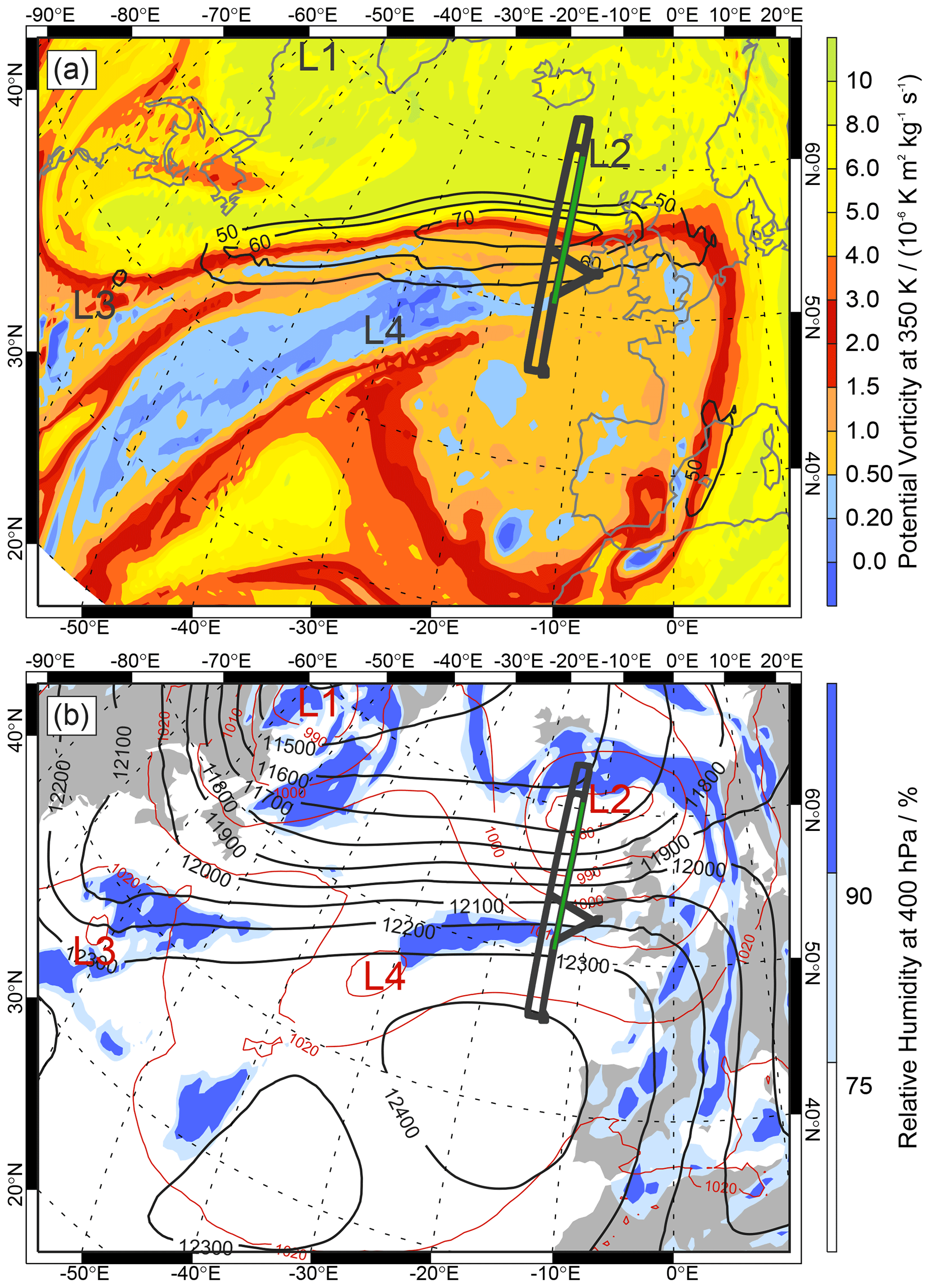
Figure 1(a) Potential vorticity (in colors; PVU) and horizontal wind speed (black contour lines; in m s−1 for >50 m s−1) at 350 K. (b) Relative humidity at 400 hPa (colors; in %), geopotential height at 150 hPa (black contour lines; in m) and surface pressure (red contour lines; in hPa) as represented in the ECMWF operational analysis on 1 October 2017, 18:00 UTC. L1–L4 mark the location of surface cyclones. Panels (a) and (b) are superimposed by the HALO flight track (12:05–21:57 UTC; thick black line) and the subsection from 18:40 to 20:00 UTC (green line) that is discussed in this paper.
Here, we focus on one particular case on 1 October 2017 that was characterized by a straight southwesterly jet stream over the North Atlantic Ocean (Fig. 1a) located between a large-scale longwave trough over the western Atlantic and a ridge extending over the North Sea into southern Scandinavia (Fig. 1b). Two surface cyclones evolved in the upstream trough (L1 and L3 in Fig. 1) that feature typical cyclonic cloud patterns at 400 hPa which are indicative of vertical transport of tropospheric air ahead of the trough. Further downstream, a surface cyclone was located between the UK and Iceland (L2) and another surface low (L4) is visible over the central North Atlantic south of the strong jet stream. The 350 K PV distribution intersects with the jet stream that follows the maximum gradient in PV (Martius et al., 2010) and separates stratospheric air (>2 PVU) north of the wind speed maximum from tropospheric air (<2 PVU) to its south. In this region of strong horizontal and vertical velocity gradients and neighboring air masses of different origin, isentropic mixing was expected to have influenced the ExTL. The synoptic pattern was found to be relatively persistent over the preceding hours. Stratospheric air was transported all around the subtropical anticyclone keeping its high levels of PV in contrast to the tropospheric low-PV air that was advected northeastward on the leading edge of the upstream longwave trough filling the center of the anticyclone (Fig. 1a).
HALO performed a flight between 12:04 and 21:57 UTC that aimed at observing predicted strong tracer gradients and mixing across the jet stream using both in situ and remote sensing instrumentation. Multiple, almost perpendicular crossings of the jet stream at 13 and 15∘ W were performed along a rectangular-shaped flight pattern at different altitudes for in situ (FL 280, FL 410, FL 430) and remote sensing measurements (FL 450, ∼14 km). In this study, we concentrate on the last jet stream transect at 13∘ W from 18:40 to 20:00 UTC (green line in Fig. 1) only, providing maximum data coverage beneath the aircraft at FL 450. As this study focuses on processes in the jet stream, the northern- and the southernmost parts of the meridional flight track were omitted. In those parts of the flight, either air mass transport in the occluded cyclone L2 or older stratospheric air that was advected around the upper-level anticyclone (Fig. 1a) were encountered which are not relevant for this study. On the considered transect between 50.5 and 60.5∘ N, HALO crossed a zonally extended cloud band related to cyclone L4 (see Figs. 1b and 2) which coincides with the jet axis on the northern side of the clouds.
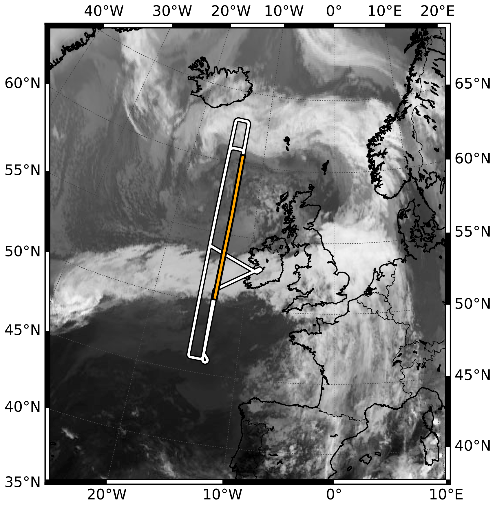
Figure 2Meteosat SEVIRI infrared satellite image (10.8 µm) for 1 October 2017 at 18:00 UTC superimposed by the HALO flight track (12:05–21:57 UTC; thick black line) and the subsection from 18:40 to 20:00 UTC (orange line). Copyright 2020 EUMETSAT.
3.2 O3 and H2O along the observed cross sections
Figure 3 shows the observed distributions of H2O and O3 along the above-described ∼1100 km long meridionally oriented cross section between 18:40 and 20:00 UTC, comprising a total of 200 lidar profiles that are shown for an altitude range between 2.5 and 14 km. In the first 400 km, the dynamical tropopause (2 PVU) is located at altitudes between 7.5 and 8.5 km before it slopes down to about 5 km altitude. At about half of the flight leg, a steep ascent of the dynamical tropopause is accompanied by tropospheric air masses reaching altitudes up to ∼14 km further south. The stratospheric air is characterized by increased static stability as is visible from the increased vertical potential temperature gradient. Westerly jet stream winds with maximum wind speeds up to 90 m s−1 at 9 km altitude and strong horizontal and vertical wind speed shear blow perpendicular to the flight track. Isentropes intersect the dynamical tropopause between 314 and 366 K of which the lowest ones extend downward in association with folding of the tropopause which is typically initiated by ageostrophic circulation around the jet stream causing an intrusion of stratospheric air (Keyser and Shapiro, 1986).
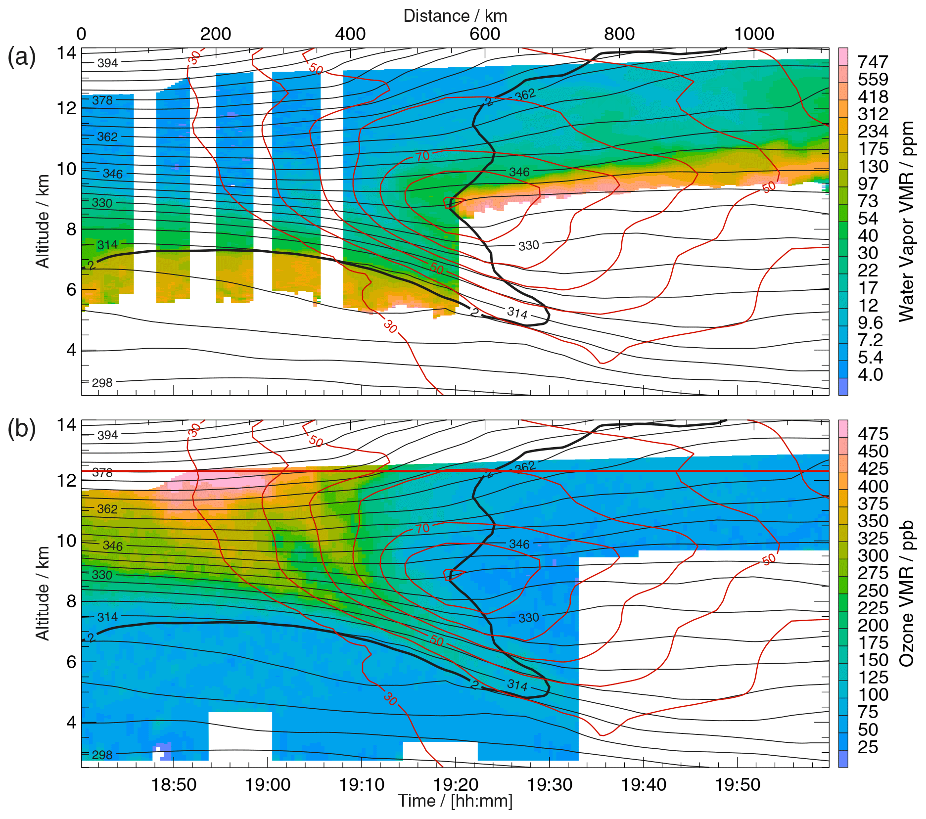
Figure 3DIAL observations (in colors) of (a) H2O volume mixing ratio (VMR; in and (b) O3 VMR (in ) on 1 October 2017 (see Fig. 1 for the flight track). Panels (a) and (b) are superimposed by horizontal wind speed (red contours; in m s−1 for wind speeds >30 m s−1), potential temperature (black contours; in K) and dynamical tropopause (2 PVU; thick black contour) interpolated from 1-hourly ECMWF ERA5 reanalyses.
H2O shows the lowest VMRs (3–7 ppm) at the highest potential temperature in the stratosphere which are typical values for autumn in the lowermost stratosphere (e.g., Zahn et al., 2014). In contrast, the highest H2O VMRs occur in the troposphere to the north and south of the jet stream ranging from ∼100 to 1000 ppm. The moist tropospheric air north of the jet stream is relatively well-mixed and provides typical autumnal values for the upper troposphere of 100–300 ppm. The high-reaching tropospheric air to the south of the jet stream is more stratified. H2O quickly decreases above a shallow (1–1.5 km) moist layer (100–1000 ppm) in the lowest part. The highest H2O VMRs are indicative of recent vertical transport (e.g., in WCBs) from the moist lower troposphere (Zahn et al., 2014). Furthermore, the stratification and some filamentary structures with enhanced H2O at upper levels suggest differential transport impacting the distribution of the upper-tropospheric air. The lowest H2O VMR (10–40 ppm) at the highest levels and the exceptionally high dynamical tropopause and potential temperatures are indicative of transport from the subtropical or tropical upper troposphere (UT). Missing data below the moist layer stem from midlevel clouds (see Figs. 1b and 2), while, in the first half of the flight, the data gap below ∼5.5 km results from attenuation of the laser signal in lower and moister air. Vertical stripes of missing H2O data are the result of cooling issues intermittently occurring at high flight altitudes with high potential temperatures.
In addition, observed O3 values represent typical concentrations for the season (cf. Krebsbach et al., 2006). In contrast to H2O, the highest O3 (O3 VMR of 300–500 ppb) was measured in the lowermost stratosphere (LMS) with a strong decrease towards lower altitudes and the south. Although the region of the highest O3 is relatively compact, it shows large inhomogeneity on smaller scales with two filamentary structures of increased VMR extending across isentropes towards the intrusion located below the jet stream where air is adiabatically transported towards the ground. In the troposphere, O3 is comparatively low (20–100 ppb) with the lowest values occurring in the mid-tropospheric moist air to the south of the jet stream being indicative of recent transport from the lower troposphere. The tropopause fold redistributes O3 and H2O with O3 decreasing and H2O increasing at its sides.
Note that only collocated data along the cross section are used in the following T–T diagnostics which covered the lower stratosphere north of the jet stream and a part of the upper troposphere on both sides. Therefore, it is well-suited to investigate the ExTL. Note that due to the presence of clouds no collocated observations are available in the lower part of the tropopause fold.
3.3 O3 and H2O as tracer–tracer correlations
In T–T space, the collocated O3 and H2O lidar measurements (Fig. 4a) form an L-shaped distribution with an arc-shaped transition in between which immediately highlights that the DIAL observations are suited to distinguish stratospheric, tropospheric and mixed air masses. In order to better characterize the partly superposed measurements, Fig. 4b shows the number of observations contributing to individual bins in the T–T diagram. O3 values of less than ∼100 ppb give a first rough depiction of the tropospheric branch that holds variable H2O with VMRs covering 4 orders of magnitude and featuring two maxima between 10 and 40 ppm and 100 and 300 ppm. The stratospheric branch is immediately identified by H2O observations with VMRs of less than ∼7 ppm. In between both branches, collections of mixing lines form compact traces with increased numbers of observations that will be called mixing regimes in the following. The arc-shaped mixing regime that is split in two traces at higher ozone concentrations connects stratospheric O3VMRs of 250–350 ppb with tropospheric H2O VMRs of 30–70 ppm. Interestingly, an area to the right of this arc-shaped mixing regime with a low number of observations suggests mixing between already mixed air and more humid (H2O VMR of 100–200 ppm) tropospheric air. The lower left area in T–T space, connecting very dry tropospheric air (H2O VMR of 8–15 ppm) and ozone-rich stratospheric air (O3VMR >250 ppb) is less obvious as it may be part of the dry and ozone-poor stratospheric branch typically originating from low-latitudes (e.g., Tilmes et al., 2010) or it may be related to the mixing of dry subtropical tropospheric air with ozone-rich stratospheric air. The former appears less likely as climatological midlatitude distributions show such pure stratospheric air masses at very low H2O only during northern hemispheric winter (Hegglin et al., 2009). Additionally, H2O is slightly increased compared to the stratospheric background with H2O VMR of 4–7 ppm (cf. Zahn et al., 2014) leading to a somewhat reduced slope compared to the stratospheric branch. Please note that the above-described tropospheric and stratospheric entry VMRs represent typical values with respect to climatology (Hegglin et al., 2009). Based on these findings, Fig. 4c introduces a classification of the observed air masses solely based on their location in T–T space for this quasi-instantaneous jet stream cross section. The light blue area covers the stratospheric branch (STRA) with VMR O3 >280 ppb and VMR H2O <7 ppm. The tropospheric branch is subdivided into three classes with slightly varying O3 thresholds depending on the measurement frequencies in Fig. 4b. TRO-1 represents the driest tropospheric air (VMR H2O <30 ppm), TRO-2 the intermediate air mass (30 ppm <VMR H2O >100 ppm) and TRO-3 the moistest air mass (VMR H2O >100 ppm). Table 1 summarizes the applied thresholds to detect tropospheric and stratospheric air. The three above-discussed mixing regimes are colored in dark green (MIX-1), green (MIX-2) and light green (MIX-3) and connect the stratospheric branch with different parts of the troposphere. The threshold between TRO-1 and TRO-2 was adapted to represent the tropospheric end of transitions within MIX-1 and MIX-2. The distribution of these air mass classes in geometrical space are further detailed in Sect. 3.4.
Table 1Thresholds used for the air mass classification of tropospheric and stratospheric air in T–T space (see also Fig. 4).
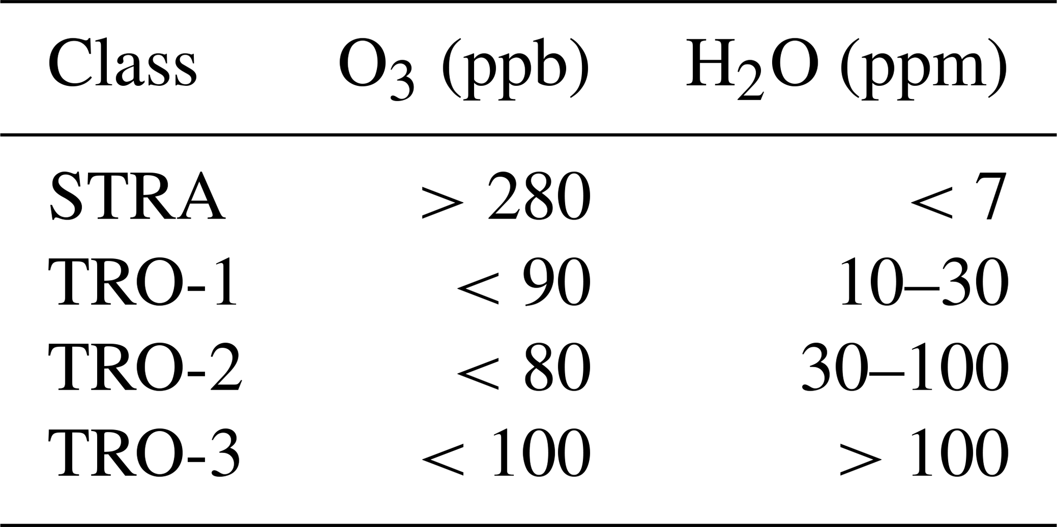
Figure 5 shows mean and variability in pressure, potential temperature and PV for each bin in the T–T diagram. STRA provides low pressures and high potential temperatures that decrease towards lower O3, which corresponds to vertically decreasing O3 values (Fig. 3b). The increased variability in pressure at lower O3 VMRs within STRA can be explained by the additional latitudinal decrease in O3 at the highest altitudes (low potential temperatures). The dry tropospheric air mass TRO-1 also provides low pressure and high potential temperature. Conversely, TRO-2 and TRO-3 possess higher pressure and lower potential temperature. The lowest tropospheric O3 corresponds to air at ∼8–10 km altitude on the southern side of the jet stream. Towards higher O3, pressure increases (potential temperature decreases) within TRO-2 and TRO-3 accompanied by increased variability which corresponds to tropospheric observations at different altitudes on the northern and southern side of the jet stream. MIX-1 features low pressures indicating that the transition occurred at high altitudes. High and relatively constant potential temperatures suggest an isentropic mixing regime within MIX-1. The lower the pressure (the higher the potential temperature) within MIX-1 was, the lower the H2O concentration was, which is expectable due to vertically decreasing tropopause temperatures that define the ExTL moisture when mixed across the jet stream (e.g., Zahn et al., 2014). Within MIX-2, pressure and its variability increase towards the tropospheric branch, while potential temperature decreases. The higher the altitude (higher potential temperature and lower pressure) was, the lower the H2O VMR and O3 VMR were observed in MIX-2. The area within MIX-2 that shows a separated and rather linear trace (Fig. 4b) features the highest potential temperature and lowest pressure. MIX-3 occurs at low potential temperatures and higher pressures.
Figure 5c shows the distribution of PV which is a tracer for stratospheric air comparable to O3 as it has comparable gradients across the tropopause with high values in the stably stratified stratosphere (e.g., Shapiro, 1980). As expected, PV is highest in STRA and strongly decreases along the mixing regimes with decreasing O3. The mixed air masses show PV values between 2 and 7 PVU. Furthermore, PV is found to be variable within the regimes in the ExTL. Therefore, it is assumed that the interrelation of the dynamical and chemical transition depends on altitude (potential temperature), a circumstance that will be discussed in more detail in Sect. 3.5. The lowest PV values are correlated with low O3 values in the troposphere indicating more recent transport from the lower troposphere.

Figure 4Tracer–tracer (T–T) correlations of O3 and H2O for the collocated DIAL data on 1 October 2017. (a) All collocated observations, (b) number of data points and (c) air mass classification for bins in T–T space (bin sizes of 10 ppb for VMR O3 and 0.05 ppm of log 10 (VMR H2O)).
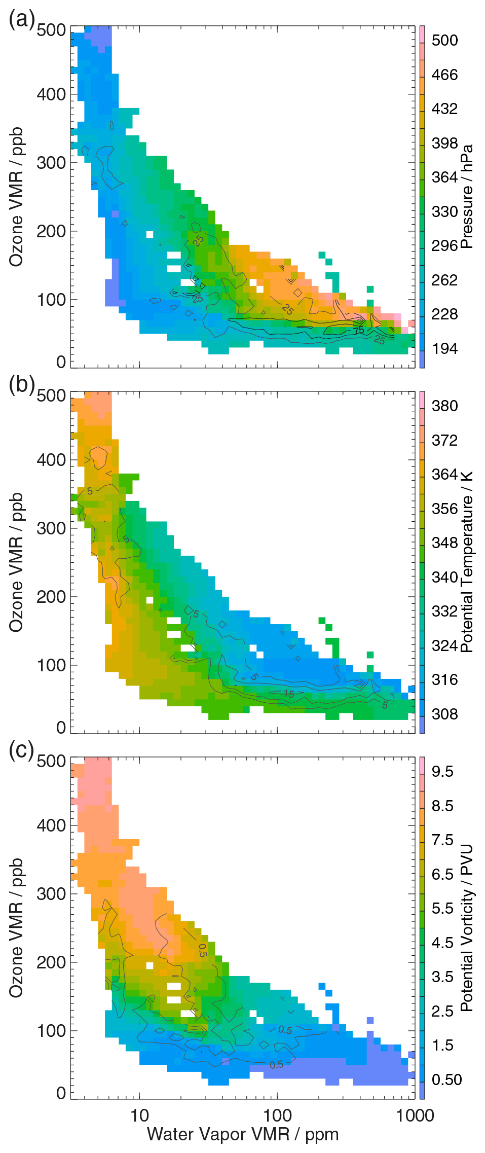
Figure 5T–T correlation as in Fig. 4b but for mean (in colors) and standard deviation (gray contours) of (a) pressure, (b) potential temperature and (c) potential vorticity.
3.4 A combined view of O3 and H2O in T–T and geometrical space
A back projection of the air mass classification from T–T space (Fig. 4c) into geometrical space along the cross section gives more detailed information on the shape and composition of the ExTL (Fig. 6). First, it is striking that the different air masses correspond to remarkably coherent areas along the cross section. The mixed air masses in the ExTL (MIX-1, MIX-2 and MIX-3) reach about ∼30 K above the dynamical tropopause in the northern part before they ascend with the rising tropopause further to the south. MIX-1 occurs at the highest altitudes in the upper part of the jet stream with its bottom being relatively well defined by the 348 K isentrope. MIX-1 connects STRA with TRO-1 (isentropic transition) which underlines the validity of considering MIX-1 as being mixed air instead of stratospheric background. The relatively constant potential temperature along the mixing regime (Fig. 5b) suggests the relevance of mixing processes in the upper-part of the jet stream.
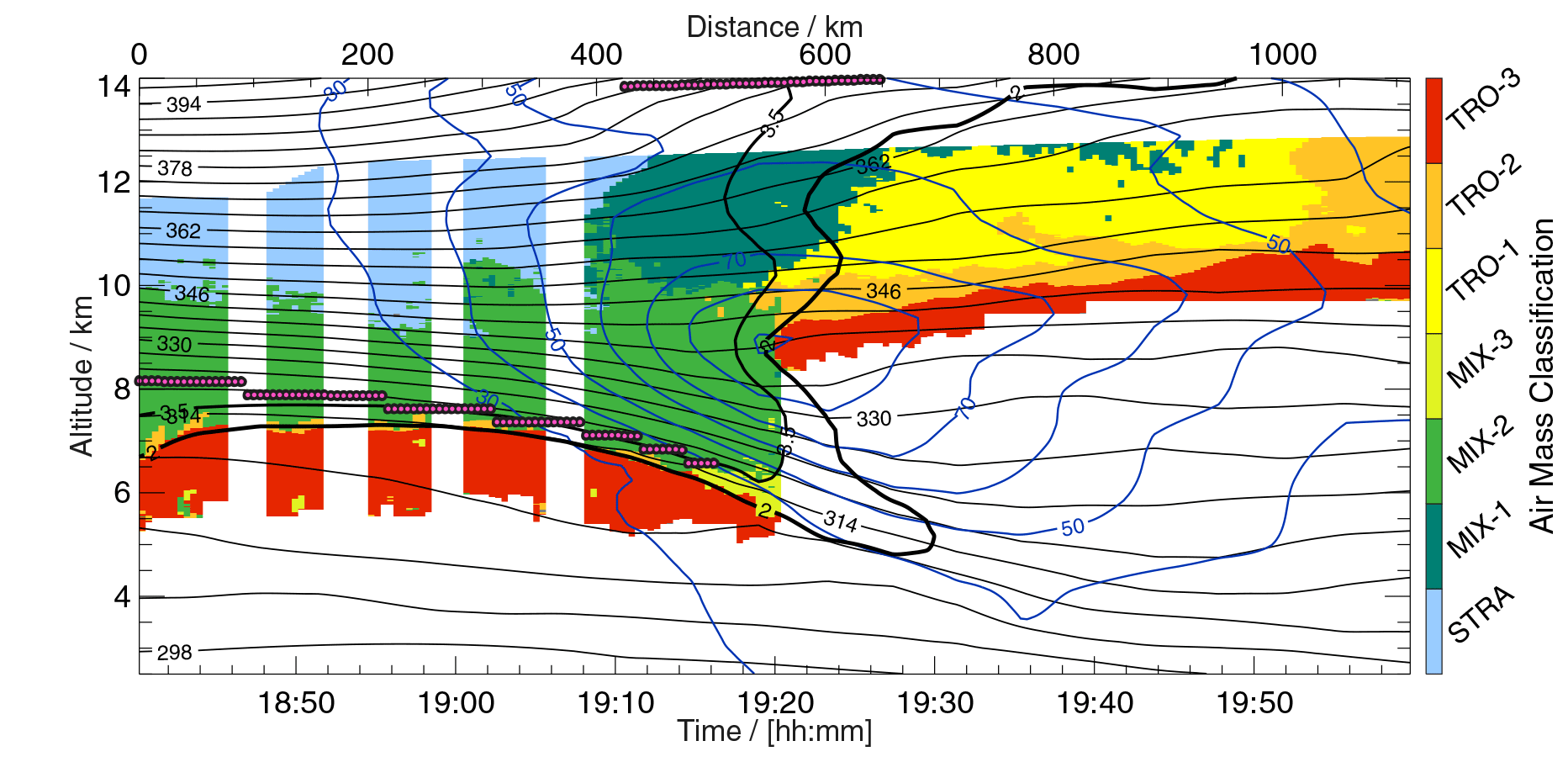
Figure 6Collocated observations colored by the air mass classification in Fig. 4c. Superimposed model information as in Fig. 3 with an additional PV contour for 3.5 PVU. Pink circles mark the thermal tropopause according to the temperature lapse rate criterion (WMO, 1957).
Below, MIX-2 comprises isentropic transitions of STRA with TRO-2 and TRO-3 above the clouds in the troposphere, as well as cross-isentropic vertical transitions in the northern part of the flight between STRA and TRO-3. In the northern part of the flight section, the bottom of the ExTL (MIX-2) agrees with the dynamical tropopause, while the thermal tropopause lies within the ExTL and approximately follows the 3.5 PVU contour. Please note that the thermal tropopause provides a typical split structure near the jet stream, while the dynamical tropopause proceeds vertically (e.g., Randel et al., 2007). The agreement of the almost vertical dynamical tropopause and the border to the tropospheric air (TRO-1–TRO-3) is less uniform, and TRO-1 and TRO-2 air masses reach into areas north of the dynamical tropopause. MIX-3 occurs in the lowest observed part of the intrusion that was observed before reaching the clouds. The geometrical location points to mixing processes between mixed ExTL air masses and the TRO-3 air mass below in the lower part of the jet stream. Note that the 348 K isentrope also separates TRO-1 from TRO-2 in the tropospheric air, which points to different source regions of humidity in the troposphere. STRA is located at the highest altitudes and in the most northern part.
To further investigate the structure and strength of stratosphere to troposphere transitions within the ExTL, the concept of the mixing degree metric firstly introduced by Kunz et al. (2009) is advantageous. It is a measure of how much an air mass deviates from the background due to mixing in its previous history and is solely based on the location of the observed air mass in T–T space. Here, we adapt this concept to the lidar data, but unlike Kunz et al. (2009), the presented mixing factor herein is only a function of distance from the undisturbed stratospheric and tropospheric background. It does not account for the distance to the intersection point of tropospheric and stratospheric branches as a mixing event is not considered to be stronger in the case of the tropospheric H2O VMR and stratospheric O3 VMR being increased. At first, dimensionless variables x and y are calculated from the VMR H2O and VMR O3 with
using the thresholds H2OMIN=6.5 ppm, H2OMAX=1000 ppm, ppb and ppb to select the mixed air mass. The observations with lower VMRs than this range are considered to be unmixed tropospheric and stratospheric air. In order to range from 0 (pure stratospheric air) to 1 (pure tropospheric air), the mixing factor f is calculated for x>y as and for x<y as .
Figure 7a shows the observations color-coded by the mixing factor. Please note that the selected ExTL air masses slightly differ from Fig. 4 due to the application of constant minimum thresholds. The back projection of the mixing factor in Fig. 7b picks up the major transition regions in MIX-1, MIX-2 and MIX-3. At the highest levels (above 350 K), i.e., directly above the jet stream maximum winds, the isentropic transition is rather uniform. In the layer beneath (340–350 K), rapid transitions result in a lack of observations with intermediate chemical characteristics. Below potential temperatures of 340 K, the transition is again more uniform. Within the tropopause fold air masses with intermediate chemical composition are transported towards the lower troposphere. The above-described stratospheric filaments of high O3 correspond to decreased mixing factors indicating the stratospheric character of the observed air compared to the surroundings. Figures 6 and 7b suggest that both vertical (MIX-2) and isentropic transitions (MIX-1 and MIX-2) formed the mixing lines.

Figure 7Mixing factor diagnostic for all collocated measurements in (a) T–T space using lower limits for H2O VMR of 6.5 ppm and for O3 VMR of 90 ppb for selecting mixed air masses (for details see text) and (b) projected back to geometrical space.
Figure 8 shows how observations in certain subregions along the lidar cross section become apparent in T–T distributions. Profiles before 19:00 UTC (Fig. 8a) represent vertical transitions in the first part of the flight that form transitions from high O3 in the stratosphere along the arc-shaped mixed region in T–T space into TRO-3 (Fig. 8b). Within the ExTL (MIX-2) the mixing lines connect comparably high stratospheric O3 (∼300 ppb) with high tropospheric H2O (∼50 ppm). The tropospheric air is rather rich in O3 and does not reach the highest levels of H2O within TRO-3. Figure 8c and d show the layer 335 to 340 K between 19:00 and 19:45 UTC, representing the above-discussed rapid transition between tropospheric and ExTL air at the level of the jet stream maximum winds connecting TRO-3 and MIX-2. Both air masses are clearly separated in T–T space with H2O VMRs jumping from ∼50 ppm at the tropospheric end of MIX-2 to ∼500 ppm in TRO-3 (Fig. 8d) over a very short spatial distance (Fig. 8c) indicating minor mixing between both air masses. The more stratospheric part of MIX-2 follows the arc-shaped distribution, while the tropospheric part that is facing the jet stream is slightly detached (Fig. 8d), which potentially indicates different mixing processes within this particular layer. Interestingly, the layer directly above (340–347 K; Fig. 8e) that represents the transition of MIX-2 air with medium moist air in TRO-2 is relatively abrupt but the discontinuity occurs within the ExTL (Fig. 8f), i.e., between the linear-shaped stratospheric part and the tropospheric end, suggesting some in-mixing of TRO-2 air into this layer. The location of these abrupt transitions in the two layers between 337 and 347 K occurs at the same spatial location (cf. Fig. 7b). Both layers do not reach far into the LMS. The situation appears different in the upper part between 349 and 358 K where the mixing factor diagnostic shows more uniform transitions (Fig. 7b). The layer that connects LMS air in STRA with low H2O VMRs in TRO-1 (Fig. 8g) shows more gradual transitions across MIX-1 in T–T space (Fig. 8h). Please note that the minimum number of observations within MIX-1 (O3 VMR 200–250 ppm) is a result of the data gap between 19:06 and 19:08 UTC. Figure 8i and j show the vertical transitions at the bottom of the tropopause fold that unlike the vertical transitions in Fig. 8a and b show a mixing of ExTL air (MIX-2) and tropospheric air (TRO-3) below.
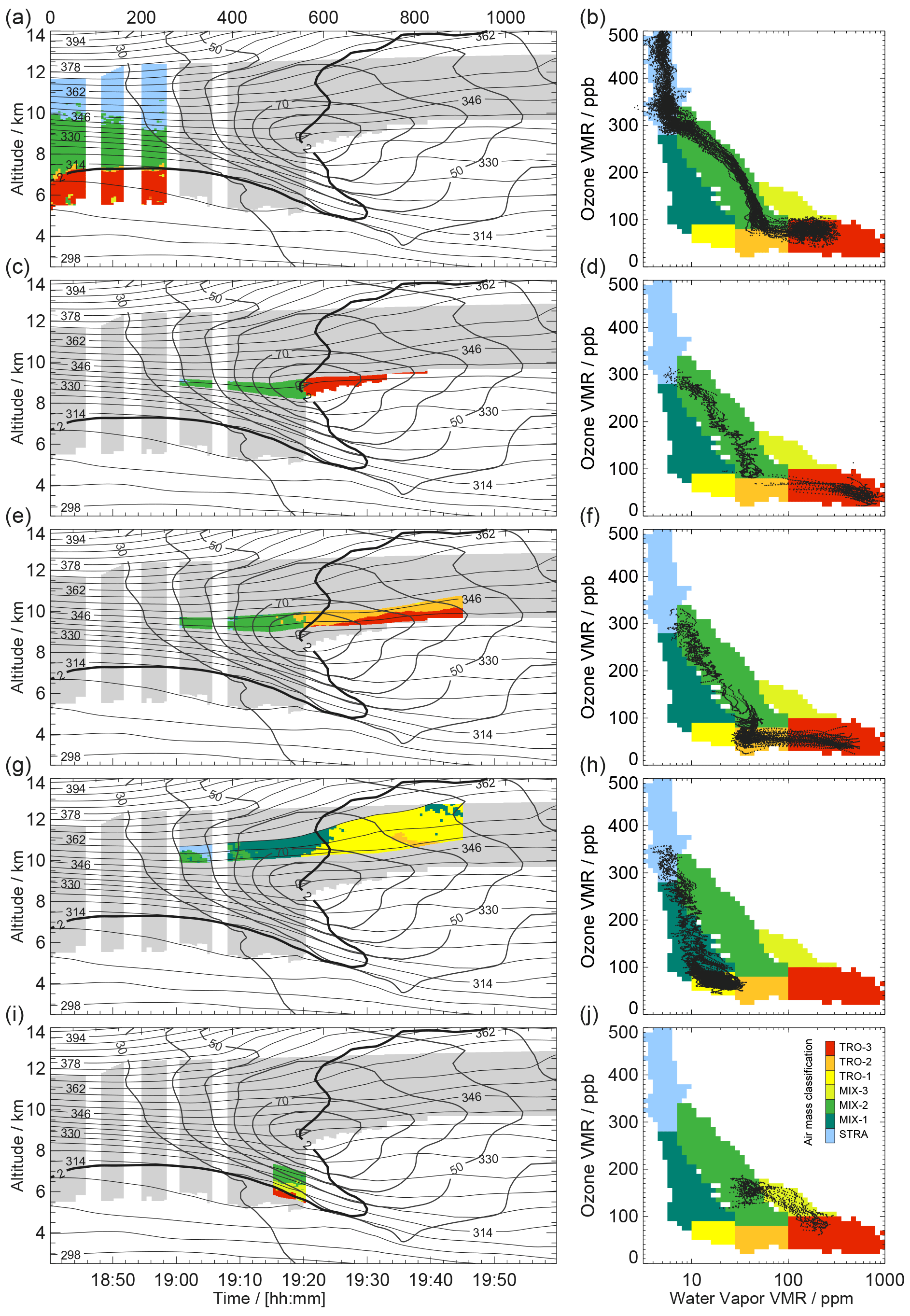
Figure 8Data subsets of the collocated lidar data. (a, b) Before 19:00 UTC with (a) showing the data as classified in Fig. 6 and in (b) as black dots superimposed on the classification of all data shown in Fig. 4c. (c, d) As (a) and (b) but for data in the time period from 19:00 to 19:45 UTC in the layer 335–340 K. (e, f) For 19:00 to 19:45 UTC and 340–347 K. (g, h) For 19:00 to 19:45 UTC and 349–358 K. (i, j) For 19:15 to 19:21 UTC and 311–324 K.
3.5 Chemical and dynamical discontinuities at the tropopause
Section 3.3 and 3.4 confirmed earlier findings that the 2 PVU dynamical tropopause marks the bottom of the ExTL north of the jet stream. However, where the dynamical tropopause is almost vertical, its location relative to the ExTL boundary is found to be variable (Fig. 6). Additionally, the mixing factor metric shown (Fig. 7b) indicates differing strengths in the ExTL transition at different layers within the jet stream. Figure 9a and b show regridded versions of the O3 and H2O cross sections using potential temperature as the vertical coordinate. As in Fig. 3a and b, all available O3 and H2O observations are used for maximum data coverage to determine isentropic gradients. Obviously, the stratospheric air with its strong vertical gradients in potential temperature gets stretched, while the tropospheric part shrinks in isentropic coordinates.
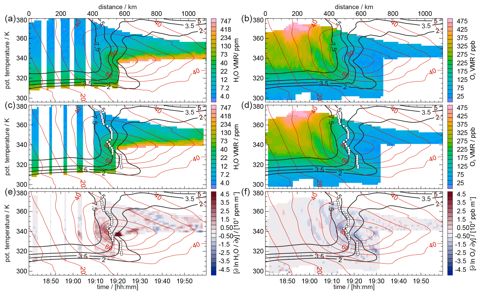
Figure 9Regridded DIAL observations of (a) H2O and (b) O3 (as shown in Fig. 3) using potential temperature as the vertical coordinate (same profile locations and for potential temperature bins of 2 K). (c, d) As (a) and (b) but using a moving average filter along isentropic levels (using 7 observations for H2O and O3 and 13 model values for PV and wind speed). Panels (e) and (f) show isentropic gradients of the natural logarithm of VMR H2O and VMR O3 based on the isentropically smoothed data. All panels are superimposed by PV contours (2, 3.5, 5 and 7.5 PVU; thick black contours) and wind speed (in m s−1 for >30 m s−1). White dots in (c)–(f) mark the PV-gradient tropopause based on maximum gradients of isentropic PV and winds following Kunz et al. (2011a) (for details see text).
The jet stream maximum is located at ∼340 K with the 2 PVU isoline crossing it. Higher PV isolines appear north of the jet. In addition to arbitrarily selected PV thresholds for the dynamical tropopause (Hoerling et al., 1991), Kunz et al. (2011a) introduced a dynamical tropopause which is defined as the maximum isentropic PV gradient which is maximized near jet streams (Martius et al., 2010). The PV-gradient tropopause is constrained by the wind speed to correctly identify high wind speed situations near polar and subtropical jet streams. Figure 9c and d depict the PV-gradient tropopause along the isentropes in the latitudinal cross section. Note that the quasi-linear interpolation between gridded model data along the 15∘ W meridian resulted in edged PV distributions on isentropes that required smoothing using a moving average. For this reason, PV contours in Fig. 9c and d appear slightly smoothed. Consistent with Kunz et al. (2011a), the PV-gradient tropopause is shifted to higher PV values with increasing potential temperature. It approximately follows the curvy shape of individual PV isolines.
To calculate isentropic trace gas gradients from the observational data, O3 and H2O are also smoothed (Fig. 9c and d) to account for instrument-generated noise causing strong local gradients. Note that smoothing of the H2O data increased the data gaps before 19:10 UTC. Trace gas gradients were then calculated for the natural logarithm of the trace gas concentration as suggested by Kunz et al. (2011b) with the purpose of scaling down increased gradients in the source regions at higher concentrations of the trace gas (stratosphere for O3 and troposphere for H2O). This shifts the focus towards the gradients across the tropopause. Strongest isentropic gradients of H2O are found at the level of maximum winds within the ExTL (MIX-2), while above H2O gradients are weaker where tropospheric H2O VMR (TRO-1) is lower and mixing within MIX-2 is more uniform (Fig. 9e and f). Please note that the highest local gradient at ∼ 19:20 UTC is related to a very high H2O VMR at the edge of the cloud layer. O3 with higher coverage in the lower part of the tropopause fold also indicates maximum gradients at the level of maximum winds. Additionally, an increased O3 gradient occurs at the bottom of the fold as compared to H2O. O3 gradients are smaller above 350 K. Some increased positive and negative gradients are found in the stratosphere related to the O3 filament. The PV-gradient tropopause better represents the regions of the highest isentropic trace gas gradients than the 2 PVU isoline, especially in the case of the O3 gradients. It follows the center of maximum O3 gradients at the level of highest wind speeds and above. Maximum H2O gradients are located north of the PV-gradient tropopause at even higher PV values at the jet stream level where pronounced gradients are visible. Kunz et al. (2011b) argue that the better agreement of the PV-gradient tropopause with the stratospheric tracer originates from their common stratospheric concept, in the sense that the chemical tracer O3 and the dynamical tracer PV are higher in the stratosphere. In contrast H2O exhibits stronger tropospheric gradients which are mostly related to transport processes into the UT.
In this study we analyze the mixing of air masses at the extratropical tropopause that shapes the structure and the chemical composition of the ExTL with the first-ever set of collocated O3 and H2O lidar observations obtained during the WISE field campaign over the North Atlantic Ocean in autumn 2017. We demonstrate the potential of quasi-instantaneous O3 and H2O cross-section observations in a dynamically rather simple synoptic situation with a perpendicular crossing of a straight southwesterly jet stream. The presented flight on 1 October 2017 captured a low tropopause on the northern cyclonic shear side of the jet stream and a high tropopause with high-reaching tropospheric air to its south. In between, a tropopause fold extended downward along tilted isentropes into the lower tropospheric frontal zone before the tropopause strongly ascended accompanied by an upper-level frontal zone above the jet stream. This flight provides exceptionally good data coverage due to low cloud coverage beneath the aircraft and a high flight altitude.
The collocated and range-resolved O3 and H2O lidar profile data along the cross section feature typical values for the season, latitude and altitude range when compared to climatological values. We show that the precision of the data at a horizontal resolution of 5.6 km is suitable to identify the ExTL and to depict its shape and composition in unprecedented detail by applying established T–T diagnostics. Through a back projection of T–T-derived information to geometrical space, i.e., along the cross section, physically meaningful thresholds were selected for the air mass classification that so far was barely possible (e.g., Pan et al., 2004). The lidar observations allow the ExTL to be determined for an individual but representative dynamic situation. The 2D depiction represents the first and almost complete observation-based illustration of the ExTL and confirmation of the conceptual model in Gettelman et al. (2011) that shows the ExTL following the tropopause. So far, this concept was based on studies using a limited number of in situ flight legs at different altitudes or model simulations (e.g., Pan et al., 2007; Vogel et al., 2011; Konopka and Pan, 2012).
We further demonstrate that probability densities in T–T space enable us to identify certain clusters of mixing lines (i.e., mixing regimes) and to classify subsets of mixed and tropospheric air. These classes show a remarkably coherent structure in geometrical space. In the upper part of the jet stream, ozone-rich stratospheric air and dry tropospheric air are connected via a distinct mixing regime. Below, a separated mixing regime links stratospheric air with moister tropospheric air. Although these mixed air masses are clearly separated in T–T space, we illustrate that they are stacked directly on top of each other in geometrical space. As the separation in the tropospheric and the mixed air occurs at the same potential temperature (∼348 K), we hypothesize that different transport pathways in this particular dynamic situation brought air with differing H2O VMRs to the upper-tropospheric end of these mixing regimes. Dry low latitude tropospheric air, being either dehydrated in the convective tropics or losing moisture through lifting to a colder and higher altitude in a tropical cyclone, arrived above moister extratropical air, typical for the warmer temperatures near the extratropical tropopause (e.g., Hegglin et al., 2009; Zahn et al., 2014). Potentially, Hurricane Maria, which was located in the tropical and subtropical western Atlantic in late September 2017 may have played a role (NOAA/NHC, 2018).
The simultaneous contribution of extra-tropical and tropical tropospheric air to mixing in the ExTL contrasts with the conceptual model of Gettelman et al. (2011) which shows distinct mixing processes at the subtropical and polar jet stream. However, our findings are in accordance with other case studies that documented large dynamical variability in transport pathways near the extratropical tropopause. A transport of low-latitude tropospheric air is also shown in the upper troposphere of a midlatitude jet stream by Vogel et al. (2011). Although our lidar observations are not covering the elevated tropopause on the anticyclonic shear side, we observed a southward extension of mixed air across the dynamical tropopause at the highest levels that agrees with their finding of enhanced upper-level mixing. In a likewise synoptic setting, Pan et al. (2007) observed a comparable separation in T–T space; however, the very low H2O with increasing O3 was of stratospheric origin in this case. The presented T–T distributions resemble the satellite-derived climatological distribution of the northern hemispheric midlatitudes (Hegglin et al., 2009). However, a clear separation of mixed air masses with low H2O beside the typical extratropical mixed air is not occurring in the more uniform climatological data that averages over a series of individual dynamic situations. Zahn et al. (2014) find an influence of tropical tropospheric air in summer that is attributed to subsiding subtropical and tropical air masses in the downward branch of the Hadley cell. Thus, this case is considered as a representative set of observations of the ExTL for the season.
We further address the question of how mixing lines in T–T space can be interpreted. Our analysis has shown compact regions in T–T space which, however, even show up in multi-week or multi-month data sets covering different meteorological situations (e.g., Pan et al., 2004; Hegglin et al., 2009). This characteristic makes the T–T method a valuable tool to determine the mean structure and composition of the ExTL. However, it raises the question of whether mixing lines for individual cross sections can be interpreted as causal physical links between the observed neighboring air masses or whether the relatively small variability in upper-tropospheric H2O and in lower-stratospheric O3 on such timescales is key to the compact distribution. It has to be mentioned that the individual location in T–T space is rather an effect of mixing events in the Lagrangian history of the observed air than an effect of instantaneous mixing that may be suggested by a snapshot taken from the lidar. Even when assuming stationarity of the flow over the past hours, as in this presented case, the observed air masses are separated over a short period of time due to the strong wind speed shear in the jet. Although the presented combination of methods does not inform about the process, the location and the time of the mixing event that formed the individual ExTL observation add some value considering the dynamical background.
We find that both vertical and horizontal transitions between tropospheric and stratospheric background air form mixing lines. Although the T–T diagram may imply direct mixing between observed air masses, it is difficult to imagine a process that physically links tropospheric and stratospheric background air with a difference in potential temperature of up to 40 K higher in the first part of the flight. This suggests that the ExTL observed in this region is influenced by advection of older mixed air. Further south, the mixing factor metric, adapted from Kunz et al. (2009), reveals uniform isentropic transitions in the upper part of the jet stream pointing to increased mixing, while the rapid transitions at the level of maximum winds indicate little mixing. This is confirmed by the consideration of data subsets which only becomes possible through the application of the novel collocated lidar data. Clearly, transitions at the level of the jet stream show jumps in T–T space over small distances along the cross section, confirming that recent mixing is expected to be rather weak. Above, the more homogeneous transitions in T–T space likely indicate more recent mixing. Although the mixing factor provides some indication of increased isentropic mixing below the jet stream, unfortunately no observations are available in the lowest part of the tropopause fold due to clouds. However, a separated mixing regime at the northern edge of the fold suggests recent mixing between ExTL and moist tropospheric air beneath. The determined regions of recent mixing above and below the jet stream fit best with the idea of quasi-instantaneous mixing which confirms and illustrates the well-established concept of turbulence-induced mixing in strong wind shear regions above and below the maximum winds in the jet stream (Danielsen, 1968; Shapiro, 1976; Esler et al., 2003; Cooper et al., 2004).
We have further investigated the relationship between chemical and dynamical discontinuities, which is important for the interpretation of transport and mixing processes between troposphere and stratosphere. In agreement with earlier findings by Pan et al. (2004), in the first part of the flight, the 2 PVU dynamical tropopause marks the lower boundary of the ExTL, while the thermal tropopause that coincides approximately with the 3.5 PVU contour is located within the ExTL. At the jet stream where the dynamical tropopause runs vertical, we provide a depiction of the lidar data and derived H2O and O3 gradients in isentropic coordinates. For the first time it is confirmed by observations that, for an individual synoptic situation, the chemical discontinuity marked by isentropic trace gas gradients is better represented by the PV-gradient tropopause (Kunz et al., 2011a) than by fixed PV thresholds used for the definition of the dynamical tropopause.
Konopka and Pan (2012) show that the ExTL formation is influenced by processes on synoptic timescales and highlight that near the jet stream processes in the last 3 d are particularly important. In a follow-up study we aim to address the question of how transport has affected the distribution of trace gases for this particular case and what timescales impact the different parts of the ExTL by adding a Lagrangian diagnostic. A combination of remote sensing data and in situ observations, e.g., of other trace gas species, as shown in Pan et al. (2006), is envisaged to help to further evaluate these results. In the future such DIAL observations of O3 and H2O may be applied to investigate various other meteorological situations and processes leading to mixing across the tropopause, e.g., above WCBs. Additionally, such 2D observations of O3 and H2O may be of high relevance for the validation of chemistry and numerical weather prediction models which suffer from a lack of operational data availability in the ExTL (Magnusson and Sandu, 2019) and rely on a realistic representation of midlatitude dynamics, accurate parametrization of sub-grid-scale mixing processes and realistic chemistry.
The lidar data used in this study are available through the HALO database (https://halo-db.pa.op.dlr.de/mission/96, WISE, 2021). We are grateful to ECMWF for granting access to the full-resolution ERA5 data. The ERA5 data have been downloaded and made available by Michael Sprenger from ETH Zurich. The ETH access to the ECMWF data is provided by the Swiss National Weather Service (MeteoSwiss). Meteosat-10 L1 data (HRIT) were provided by EUMETSAT via EUMETCast.
AS designed the study, performed the data analysis, produced the figures and wrote the text. MW performed the data analysis of the DIAL water vapor and ozone data. AF performed DIAL observations during WISE. MW and AF advised on the analysis, contributed with ideas, helped with the interpretation of the data and commented on the paper.
The authors declare that they have no conflict of interest.
This article is part of the special issue “WISE: Wave-driven isentropic exchange in the extratropical upper troposphere and lower stratosphere (ACP/AMT/WCD inter-journal SI)”. It is not associated with a conference.
The authors thank the WISE PIs and the flight planning team for supporting the remote sensing contribution to the campaign and for giving us insight into a new field of research. We are grateful to DLR for supporting this work in the framework of the DLR project “Klimarelevanz von atmosphärischen Spurengasen, Aerosolen und Wolken” (KliSAW). Additionally, we thank the German Science Foundation (DFG) for supporting the HALO contribution to the WISE campaign within the priority program SPP1294 HALO. We thank our colleagues Florian Ewald for creating the satellite image and Heidi Huntrieser for her valuable comments on the manuscript.
The article processing charges for this open-access publication were covered by a Research Centre of the Helmholtz Association.
This paper was edited by Mathias Palm and reviewed by Laura Pan and one anonymous referee.
Appenzeller, C., Davies, H. C., and Norton, W. A.: Fragmentation of stratospheric intrusions, J. Geophys. Res.-Atmos., 101, 1435–1456, https://doi.org/10.1029/95JD02674, 1996.
Boothe, A. C. and Homeyer, C. R.: Global large-scale stratosphere–troposphere exchange in modern reanalyses, Atmos. Chem. Phys., 17, 5537–5559, https://doi.org/10.5194/acp-17-5537-2017, 2017.
Brenninkmeijer, C. A. M., Crutzen, P., Boumard, F., Dauer, T., Dix, B., Ebinghaus, R., Filippi, D., Fischer, H., Franke, H., Frieß, U., Heintzenberg, J., Helleis, F., Hermann, M., Kock, H. H., Koeppel, C., Lelieveld, J., Leuenberger, M., Martinsson, B. G., Miemczyk, S., Moret, H. P., Nguyen, H. N., Nyfeler, P., Oram, D., O'Sullivan, D., Penkett, S., Platt, U., Pupek, M., Ramonet, M., Randa, B., Reichelt, M., Rhee, T. S., Rohwer, J., Rosenfeld, K., Scharffe, D., Schlager, H., Schumann, U., Slemr, F., Sprung, D., Stock, P., Thaler, R., Valentino, F., van Velthoven, P., Waibel, A., Wandel, A., Waschitschek, K., Wiedensohler, A., Xueref-Remy, I., Zahn, A., Zech, U., and Ziereis, H.: Civil Aircraft for the regular investigation of the atmosphere based on an instrumented container: The new CARIBIC system, Atmos. Chem. Phys., 7, 4953–4976, https://doi.org/10.5194/acp-7-4953-2007, 2007.
Browell, E. V., Danielsen, E. F., Ismail, S., Gregory, G. L., and Beck, S. M.: Tropopause fold structure determined from airborne lidar and in situ measurements, J. Geophys. Res., 92, 2112–2120, https://doi.org/10.1029/JD092iD02p02112, 1987.
Browell, E. V., Ismail, S., and Grant, W. B.: Differential absorption lidar (DIAL) measurements from air and space, Appl. Phys., 67B, 399–410, https://doi.org/10.1007/s003400050523, 1998.
Browning, K. A., Hardman, M. E., Harrold, T. W., and Pardoe, C. W.: Structure of rainbands within a mid-latitude depression, Q. J. Roy. Meteor. Soc., 99, 215–231, 1973.
Cooper, O., Forster, C., Parrish, D., Dunlea, E., Hübler, G., Fehsenfeld, F., Holloway, J., Oltmans, S., Johnson, B., Wimmers, A., and Horowitz, L.: On the life cycle of a stratospheric intrusion and its dispersion into polluted warm conveyor belts, J. Geophys. Res., 109, D23S09, https://doi.org/10.1029/2003JD004006, 2004.
Danielsen, E. F.: Stratospheric-tropospheric exchange based on radioactivity, ozone and potential vorticity, J. Atmos. Sci., 25, 502–518, 1968.
Danielsen, E. F., Hipskind, R. S., Gaines, S. E., Sachse, G. W., Gregory, G. L., and Hill, G. F.: Three-dimensional analysis of potential vorticity associated with tropopause folds and observed variations of ozone and carbon monoxide, J. Geophys. Res., 92, 2103–2111, https://doi.org/10.1029/JD092iD02p02103, 1987.
Ehret, G., Hoinka, K. P., Stein, J., Fix, A., Kiemle, C., and Poberaj, G.: Low stratospheric water vapour measured by an airborne DIAL, J. Geophys. Res.-Atmos., 104, 31351–31359, https://doi.org/10.1029/1999JD900959, 1999.
Esler, J. G., Haynes, P. H., Law, K. S., Barjat, H., Dewey, K., Kent, J., Schmitgen, S., and Brough, N.: Transport and mixing between airmasses in cold frontal regions during Dynamics and Chemistry of Frontal Zones (DCFZ), J. Geophys. Res., 108, 4142, https://doi.org/10.1029/2001JD001494, 2003.
Fischer, H., Wienhold, F. G., Hoor, P., Bujok, O., Schiller, C., Siegmund, P., Ambaum, M., Scheeren, H. A., and Lelieveld, J.: Tracer correlations in the northern high latitude lowermost stratosphere: Influence of cross-tropopause mass exchange, Geophys. Res. Lett., 27, 97–100, https://doi.org/10.1029/1999GL010879, 2000.
Fix, A., Steinebach, F., Wirth, M., Schäfler, A., and Ehret, G.: Development and application of an airborne differential absorption lidar for the simultaneous measurement of ozone and water vapor profiles in the tropopause region, Appl. Optics, 58, 5892–5900, 2019.
Gettelman, A., Hoor, P., Pan, L. L., Randel, W. J., Hegglin, M. I., and Birner, T.: The extratropical upper troposphere and lower stratosphere, Rev. Geophys., 49, RG3003, https://doi.org/10.1029/2011RG000355, 2011.
Gray, S. L.: A case study of stratosphere to troposphere transport: The role of convective transport and the sensitivity to model resolution, J. Geophys. Res.-Atmos., 108, 4590, https://doi.org/10.1029/2002JD003317, 2003.
Gray, S., Dunning, C., Methven, J., Masato, G., and Chagnon, J.: Systematic model forecast error in Rossby wave structure, Geophys. Res. Lett., 41, 2979–2987, https://doi.org/10.1002/2014GL059282, 2014.
Hegglin, M. I., Boone, C. D., Manney, G. L., Shepherd, T. G., Walker, K. A., Bernath, P. F., Daffer, W. H., Hoor, P., and Schiller, C.: Validation of ACE-FTS satellite data in the upper troposphere/lower stratosphere (UTLS) using non-coincident measurements, Atmos. Chem. Phys., 8, 1483–1499, https://doi.org/10.5194/acp-8-1483-2008, 2008.
Hegglin, M. I., Boone, C. D., Manney, G. L., and Walker, K. A.: A global view of the extratropical tropopause transition layer from Atmospheric Chemistry Experiment Fourier Transform Spectrometer O3, H2O, and CO, J. Geophys. Res.-Atmos., 114, D00B11, https://doi.org/10.1029/2008JD009984, 2009.
Hersbach, H., Bell, B., Berrisford, P., Hirahara, S., Horányi, A., Muñoz-Sabater, J., Nicolas, J., Peubey, C., Radu, R., Schepers, D., Simmons, A., Soci, C., Abdalla, S., Abellan, X., Balsamo, G., Bechtold, P., Biavati, G., Bidlot, J., Bonavita, M., De Chiara, G., Dahlgren, P., Dee, D., Diamantakis, M., Dragani, R., Flemming, J., Forbes, R., Fuentes, M., Geer, A., Haimberger, L., Healy, S., Hogan, R. J., Hólm, E., Janisková, M., Keeley, S., Laloyaux, P., Lopez, P., Lupu, C., Radnoti, G., de Rosnay, P., Rozum, I., Vamborg, F., Villaume, S., and Thépaut, J.-N.: The ERA5 global reanalysis, Q. J. Roy. Meteor. Soc., 146, 1999–2049, https://doi.org/10.1002/qj.3803, 2020.
Hintsa, E. J., Boerling, K. A., Weinstock, E. M., Anderson, J. G., Gary, B. L., Pfister, L., Daube, B. C., Wofsy, S. C., Loewenstein, M., Podolske, J. R., Margitan, J. J., and Bui, T. P.: Troposphere-to-stratosphere transport in the lowermost stratosphere from measurements of H2O, CO2, N2O and O3, Geophys. Res. Lett., 25, 2655–2658, https://doi.org/10.1029/98GL01797, 1998.
Hoerling, M. P., Schaack, T. K., and Lenzen, A. J.: Global Objective Tropopause Analysis, Mon. Weather Rev., 119, 1816–1831, https://doi.org/10.1175/1520-0493(1991)119<1816:GOTA>2.0.CO;2, 1991.
Holton, J. R., Haynes, P. H., McIntyre, M. E., Douglass, A. R., Rood, R. B., and Pfister L.: Stratosphere-troposphere exchange, Rev. Geophys., 33, 403–439, https://doi.org/10.1029/95RG02097, 1995.
Hoor, P., Fischer, H., Lange, L., Lelieveld, J., and Brunner, D.: Seasonal variations of a mixing layer in the lowermost stratosphere as identified by the CO−O3 correlation from in situ measurements, J. Geophys. Res.-Atmos., 107, 4044, https://doi.org/10.1029/2000JD000289, 2002.
Hoor, P., Gurk, C., Brunner, D., Hegglin, M. I., Wernli, H., and Fischer, H.: Seasonality and extent of extratropical TST derived from in-situ CO measurements during SPURT, Atmos. Chem. Phys., 4, 1427–1442, https://doi.org/10.5194/acp-4-1427-2004, 2004.
Huntrieser, H., Lichtenstern, M., Scheibe, M., Aufmhoff, H., Schlager, H., Pucik, T., Minikin, A., Weinzierl, B., Heimerl, K., Fütterer, D., Rappenglück, B., Ackermann, L., Pickering, K. E., Cummings, K. A., Biggerstaff, M. I., Betten, D. P., Honomichl, S., and Barth, M. C.: On the origin of pronounced O3 gradients in the thunderstorm outflow region during DC3, J. Geophys. Res.-Atmos., 121, 6600–6637, https://doi.org/10.1002/2015jd024279, 2016.
Keyser, D. and Shapiro, M.: A review of the structure and dynamics of upper-level frontal zones, Mon. Weather Rev., 114, 452–499, https://doi.org/10.1175/1520-0493(1986)114<0452:AROTSA>2.0.CO;2, 1986.
Kiemle, C., Wirth, M., Fix, A., Rahm, S., Corsmeier, U., and Di Girolamo, P.: Latent heat flux measurements over complex terrain by airborne water vapour and wind lidars, Q. J. Roy. Meteor. Soc., 137, 190–203, https://doi.org/10.1002/qj.757, 2011.
Konopka, P. and Pan, L. L.: On the mixing-driven formation of the Extratropical Transition Layer (ExTL), J. Geophys. Res.-Atmos., 117, D18301, https://doi.org/10.1029/2012JD017876, 2012.
Kooi, S., Fenn, M., Ismail, S., Ferrare, R., Hair, J., Browell, E., Notari, A., Butler, C., Burton, S., and Simpson, S.: Airborne LIDAR Measurements of Water Vapor, Ozone, Clouds, and Aerosols in the Tropics Near Central America During the TC4 Experiment, 24th International Laser Radar Conference, 23–27 June 2008, Boulder, Colorado, United States, available at: https://ntrs.nasa.gov/search.jsp?R=20080023791 (last access: 29 March 2021), 2008.
Krautstrunk, M. and Giez, A.: The transition from FALCON to HALO era airborne atmospheric research, in: Atmospheric Physics: Background – Methods – Trends, edited by: Schumann, U., Springer-Verlag, Berlin, 609–624, 2012.
Krebsbach, M., Schiller, C., Brunner, D., Günther, G., Hegglin, M. I., Mottaghy, D., Riese, M., Spelten, N., and Wernli, H.: Seasonal cycles and variability of O3 and H2O in the UT/LMS during SPURT, Atmos. Chem. Phys., 6, 109–125, https://doi.org/10.5194/acp-6-109-2006, 2006.
Kunkel, D., Hoor, P., Kaluza, T., Ungermann, J., Kluschat, B., Giez, A., Lachnitt, H.-C., Kaufmann, M., and Riese, M.: Evidence of small-scale quasi-isentropic mixing in ridges of extratropical baroclinic waves, Atmos. Chem. Phys., 19, 12607–12630, https://doi.org/10.5194/acp-19-12607-2019, 2019.
Kunz, A., Konopka, P., Müller, R., Pan, L. L., Schiller, C., and Rohrer, F.: High static stability in the mixing layer above the extratropical tropopause, J. Geophys. Res.-Atmos., 114, 1–9, https://doi.org/10.1029/2009JD011840, 2009.
Kunz, A., Konopka, P., Müller, R., and Pan, L. L.: Dynamical tropopause based on isentropic potential vorticity gradients, J. Geophys. Res., 116, D01110, https://doi.org/10.1029/2010JD014343, 2011a.
Kunz, A., Pan, L. L., Konopka, P., Kinnison, D. E., and Tilmes, S.: Chemical and dynamical discontinuity at the extratropical tropopause based on START08 and WACCM analyses, J. Geophys. Res., 116, D24302, https://doi.org/10.1029/2011JD016686, 2011b.
Lang, A. A. and Martin, J. E.: The structure and evolution of lower stratospheric frontal zones, Part 1: Examples in northwesterly and southwesterly flow, Q. J. Roy. Meteor. Soc., 138, 1350–1365, https://doi.org/10.1002/qj.843, 2012.
Magnusson, L. and Sandu, I.: Experts review synergies between observational campaigns and weather forecasting, ECMWF Newsletter, No. 161, ECMWF, Reading, United Kingdom, available at: https://www.ecmwf.int/sites/default/files/elibrary/2019/19263-newsletter-no-161-autumn-2019.pdf (last access: 29 March 2021), 2019.
Martius, O., Schwierz, C., and Davies, H. C.: Tropopause-Level Waveguides, J. Atmos. Sci., 67, 866–879, https://doi.org/10.1175/2009JAS2995.1, 2010.
NOAA/NHC: National Hurricane Center Tropical Cyclone Report – Hurricane Maria (AL152017), available at: https://www.nhc.noaa.gov/data/tcr/AL152017_Maria.pdf (last access: 29 March 2021), 2018.
Oelhaf, H., Sinnhuber, B., Woiwode, W., Bönisch, H., Bozem, H., Engel, A., Fix, A., Friedl-Vallon, F., Grooß, J., Hoor, P., Johansson, S., Jurkat-Witschas, T., Kaufmann, S., Krämer, M., Krause, J., Kretschmer, E., Lörks, D., Marsing, A., Orphal, J., Pfeilsticker, K., Pitts, M., Poole, L., Preusse, P., Rapp, M., Riese, M., Rolf, C., Ungermann, J., Voigt, C., Volk, C. M., Wirth, M., Zahn, A., and Ziereis, H.: POLSTRACC: Airborne Experiment for Studying the Polar Stratosphere in a Changing Climate with the High Altitude and Long Range Research Aircraft (HALO), B. Am. Meteorol. Soc., 100, 2634–2664, https://doi.org/10.1175/BAMS-D-18-0181.1, 2019.
Pan, L. L., Randel, W. J., Gary, B. L., Mahoney, M. J., and Hintsa, E. J.: Definitions and sharpness of the extratropical tropopause: A trace gas perspective, J. Geophys. Res.-Atmos., 109, D23103, https://doi.org/10.1029/2004JD004982, 2004.
Pan, L. L., Konopka, P., and Browell, E. V.: Observations and model simulations of mixing near the extratropical tropopause, J. Geophys. Res., 111, D05106, https://doi.org/10.1029/2005JD006480, 2006.
Pan, L. L., Bowman, K. P., Shapiro, M., Randel, W. J., Gao, R. S., Campos, T., Davis, C., Schauffler, S., Ridley, B. A., Wei, J. C., and Barnet, C.: Chemical behavior of the tropopause observed during the Stratosphere-Troposphere Analyses of Regional Transport experiment, J. Geophys. Res.-Atmos., 112, D18110, https://doi.org/10.1029/2007JD008645, 2007.
Pan, L. L., Homeyer, C. R., Honomochi, S., Ridley, B. A., Weisman, M., Barth, M. C., Hair, J. W., Fenn, M. A., Butler, C., Diskin, G. S., Crawford, J. H., Ryerson, T. B., Pollack, I., Peischl, J., and Huntrieser, H.: Thunderstorms enhance tropospheric ozone by wrapping and shedding stratospheric air, Geophys. Res. Lett., 41, 7785–7790, https://doi.org/10.1002/2014GL061921, 2014a.
Pan, L. L., Paulik L. C., Honomichl, S. B., Munchak, L. A., Bian, J., Selkirk, H. B., and Vömel, H.: Identification of the tropical tropopause transition layer using the ozone-water vapour relationship, J. Geophys. Res.-Atmos., 119, 3586–3599, https://doi.org/10.1002/2013JD020558, 2014b.
Pan, L. L., Honomichl, S. B., Bui, T. V., Thornberry, T., Rollins, A., Hintsa, E., and Jensen, E. J.: Lapse Rate or Cold Point: The Tropical Tropopause Identified by In Situ Trace Gas Measurements, Geophys. Res. Lett., 45, 10756–10763, https://doi.org/10.1029/2018GL079573, 2018.
Randel, W. J., Seidel, D. J., and Pan, L. L.: Observational characteristics of double tropopauses, J. Geophys. Res., 112, D07309, https://doi.org/10.1029/2006JD007904.0020, 2007.
Reutter, P., Škerlak, B., Sprenger, M., and Wernli, H.: Stratosphere–troposphere exchange (STE) in the vicinity of North Atlantic cyclones, Atmos. Chem. Phys., 15, 10939–10953, https://doi.org/10.5194/acp-15-10939-2015, 2015.
Riese, M., Ploeger, F., Rap, A., Vogel, B., Konopka, P., Dameris, M., and Forster, P.: Impact of uncertainties in atmospheric mixing on simulated UTLS composition and related radiative effects, J. Geophys. Res.-Atmos., 117, D16305, https://doi.org/10.1029/2012JD017751, 2012.
Schäfler A., Dörnbrack A., Kiemle C., Rahm S., and Wirth M.: Tropospheric water vapour transport as determined from airborne lidar measurements, J. Atmos. Ocean. Tech., 27, 2017–2030, 2010.
Schäfler, A. and Harnisch, F.: Impact of the inflow moisture on the evolution of a warm conveyor belt, Q. J. Roy. Meteor. Soc., 141, 299–310, https://doi.org/10.1002/qj.2360, 2015.
Schäfler, A., Craig, G., Wernli, H., Arbogast, P., Doyle, J. D., McTaggart-Cowan, R., Methven, J., Rivière, G., Ament, F., Boettcher, M., Bramberger, M., Cazenave, Q., Cotton, R., Crewell, S., Delanoë, J., Dörnbrack, A., Ehrlich, A., Ewald, F., Fix, A., Grams, C. M., Gray, S. L., Grob, H., Groß, S., Hagen, M., Harvey, B., Hirsch, L., Jacob, M., Kölling, T., Konow, H., Lemmerz, C., Lux, O., Magnusson, L., Mayer, B., Mech, M., Moore, R., Pelon, J., Quinting, J., Rahm, S., Rapp, M., Rautenhaus, M., Reitebuch, O., Reynolds, C. A., Sodemann, H., Spengler, T., Vaughan, G., Wendisch, M., Wirth, M., Witschas, B., Wolf, K., and Zinner, T.: The North Atlantic Waveguide and Downstream Impact Experiment, B. Am. Meteorol. Soc., 99, 1607–1637, https://doi.org/10.1175/BAMS-D-17-0003.1, 2018.
Schäfler, A., Harvey, B., Methven, J., Doyle, J. D., Rahm, S., Reitebuch, O., Weiler, F., and Witschas B.: Observation of jet stream winds during NAWDEX and characterization of systematic meteorological analysis error, Mon. Weather Rev., 148, 2889–2907, https://doi.org/10.1175/MWR-D-19-0229.1, 2020.
Shapiro, M. A.: The role of turbulent heat flux in the generation of potential vorticity of upper-level jet stream systems, Mon. Weather Rev., 104, 892–906, 1976.
Shapiro, M. A.: Turbulent Mixing within Tropopause Folds as a Mechanism for the Exchange of Chemical Constituents between the Stratosphere and Troposphere, J. Atmos. Sci., 37, 994–1004, https://doi.org/10.1175/1520-0469(1980)037h0994:TMWTFAi2.0.CO;2, 1980.
Škerlak, B., Sprenger, M., and Wernli, H.: A global climatology of stratosphere–troposphere exchange using the ERA-Interim data set from 1979 to 2011, Atmos. Chem. Phys., 14, 913–937, https://doi.org/10.5194/acp-14-913-2014, 2014.
Spreitzer, E., Attinger, R., Boettcher, M., Forbes, R., Wernli, H., and Joos, H.: Modification of Potential Vorticity near the Tropopause by Nonconservative Processes in the ECMWF Model, J. Atmos. Sci., 76, 1709–1726, https://doi.org/10.1175/JAS-D-18-0295.1, 2019.
Sprenger, M. and Wernli, H.: A northern hemispheric climatology of cross-tropopause exchange for the ERA15 time period (1979–1993), J. Geophys. Res.-Atmos., 108, 8521, https://doi.org/10.1029/2002JD002636, 2003.
Stohl, A., Bonasoni, P., Cristofanelli, P., Collins, W., Feichter, J., Frank, A., Forster, C., Gerasopoulos, E., Gaggeler, H., James, P., Kentarchos, T., Kromp-Kolb, H., Kruger, B., Land, C., Meloen, J., Papayannis, A., Priller, A., Seibert, P., Sprenger, M., Roelofs, G. J., Scheell, H., E. Schnabel, C., Siegmund, P., Tobler, L., Trickl, T., Wernli, H., Wirth, V., Zanis, P., and Zerefos, C.: Stratosphere-troposphere exchange: A review, and what we have learned from STACCATO, J. Geophys. Res.-Atmos., 108, 8516, https://doi.org/10.1029/2002JD002490, 2003.
Tilmes, S., Pan, L. L., Hoor, P., Atlas, E., Avery, M. A., Campos, T., Christensen, L. E., Diskin, G. S., Gao, R.-S., Herman, R. L., Hintsa, E. J., Loewenstein, M., Lopez, J., Paige, M. E., Pittman, J. V., Podolske, J. R., Proffitt, M. R., Sachse, G. W., Schiller, C., Schlager, H., Smith, J., Spelten, N., Webster, C., Weinheimer, A., and Zondlo, M. A.: An aircraft-based upper roposphere lower stratosphere O3, CO, and H2O climatology for the Northern Hemisphere, J. Geophys. Res.-Atmos., 115, https://doi.org/10.1029/2009JD012731, 2010.
Trickl, T., Vogelmann, H., Fix, A., Schäfler, A., Wirth, M., Calpini, B., Levrat, G., Romanens, G., Apituley, A., Wilson, K. M., Begbie, R., Reichardt, J., Vömel, H., and Sprenger, M.: How stratospheric are deep stratospheric intrusions? LUAMI 2008, Atmos. Chem. Phys., 16, 8791–8815, https://doi.org/10.5194/acp-16-8791-2016, 2016.
Ungermann, J., Pan, L. L., Kalicinsky, C., Olschewski, F., Knieling, P., Blank, J., Weigel, K., Guggenmoser, T., Stroh, F., Hoffmann, L., and Riese, M.: Filamentary structure in chemical tracer distributions near the subtropical jet following a wave breaking event, Atmos. Chem. Phys., 13, 10517–10534, https://doi.org/10.5194/acp-13-10517-2013, 2013.
Urbanek, B., Groß, S., Schäfler, A., and Wirth, M.: Determining stages of cirrus evolution: a cloud classification scheme, Atmos. Meas. Tech., 10, 1653–1664, https://doi.org/10.5194/amt-10-1653-2017, 2017.
Vogel, B., Pan, L. L., Konopka, P., Günther, G., Müller, R., Hall, W., Campos, T., Pollack, I., Weinheimer, A., Wei, J., Atlas, E. L., and Bowman, K. P.: Transport pathways and signatures of mixing in the extratropical tropopause region derived from Lagrangian model simulations, J. Geophys. Res., 116, D05306, https://doi.org/10.1029/2010JD014876, 2011.
Wernli, H. and Bourqui, M.: A Lagrangian 1 year climatology of (deep) cross-tropopause exchange in the extratropical Northern Hemisphere, J. Geophys. Res.-Atmos., 107, ACL 13–1–ACL13–16, https://doi.org/10.1029/2001JD000812, 2000.
Wernli, H. and Davies, H. C.: A lagrangian-based analysis of extratropical cyclones, I: The method and some applications, Q. J. Roy. Meteor. Soc., 123, 467–489, https://doi.org/10.1002/qj.49712353811, 1997.
Wirth, M., Fix, A., Mahnke, P., Schwarzer, H., Schrandt, F., and Ehret, G.: The airborne multi-wavelength water vapour differential absorption lidar WALES: system design and performance, Appl. Phys. B, 201–213, https://doi.org/10.1007/s00340-009-3365-7, 2009.
WISE: Wave-driven ISentropic Exchange, HALO database, available at: https://halo-db.pa.op.dlr.de/mission/96, last access: 29 March 2021.
Woiwode, W., Dörnbrack, A., Bramberger, M., Friedl-Vallon, F., Haenel, F., Höpfner, M., Johansson, S., Kretschmer, E., Krisch, I., Latzko, T., Oelhaf, H., Orphal, J., Preusse, P., Sinnhuber, B.-M., and Ungermann, J.: Mesoscale fine structure of a tropopause fold over mountains, Atmos. Chem. Phys., 18, 15643–15667, https://doi.org/10.5194/acp-18-15643-2018, 2018.
World Meteorological Organization (WMO), Meteorology – A three-dimensional science, WMO Bull., 6, 134–138, 1957.
Zahn, A. and Brenninkmeijer, C.: New directions: a chemical tropopause defined, Atmos. Environ., 37, 439–440, 2003.
Zahn, A., Christner, E., van Velthoven, P. F. J., Rauthe-Schoch, A., and Brenninkmeijer, C. A. M.: Processes controlling water vapor in the upper troposphere/lowermost stratosphere: An analysis of 8 years of monthly measurements by the IAGOS-CARIBIC observatory, J. Geophys. Res.-Atmos., 119, 11505–11525, https://doi.org/10.1002/2014JD021687, 2014.
Zierl, B. and Wirth, V.: The influence of radiation on tropopause behavior and stratosphere-troposphere exchange in an upper tropospheric anticyclone, J. Geophys. Res.-Atmos., 102, 23883–23894, https://doi.org/10.1029/97JD01667, 1997.