Aerosol dynamics and dispersion of radioactive particles

In the event of a failure of a nuclear power plant with release of radioactive material into the atmosphere, dispersion modelling is used to understand how the released radioactivity is spread. For the dispersion of particles, Lagrangian particle dispersion models (LPDMs) are commonly used, in which model particles, representing the released material, are transported through the atmosphere. These model particles are usually inert and undergo only first-order processes such as dry deposition and simplified wet deposition along the path through the atmosphere. Aerosol dynamic processes including coagulation, condensational growth, chemical interactions, formation of new particles and interaction with new aerosol sources are usually neglected in such models. The objective of this study is to analyse the impact of these advanced aerosol dynamic processes if they were to be included in LPDM simulations for use in radioactive preparedness. In this investigation, a fictitious failure of a nuclear power plant is studied for three geographically and atmospherically different sites. The incident was simulated with a Lagrangian single-trajectory box model with a new simulation for each hour throughout a year to capture seasonal variability of meteorology and variation in the ambient aerosol. (a) We conclude that modelling of wet deposition by incorporating an advanced cloud parameterization is advisable, since it significantly influence simulated levels of airborne and deposited activity including radioactive hotspots, and (b) we show that inclusion of detailed ambient-aerosol dynamics can play a large role in the model result in simulations that adopt a more detailed representation of aerosol–cloud interactions. The results highlight a potential necessity for implementation of more detailed representation of general aerosol dynamic processes into LPDMs in order to cover the full range of possible environmental characteristics that can apply during a release of radionuclides into the atmosphere.

1 Introduction

Atmospheric dispersion models are used to simulate how various kinds of pollutants disperse in the atmosphere. Dispersion models for emergency preparedness and more specifically Lagrangian particle dispersion models (LPDMs) currently have very simplified descriptions of the complex aerosol dynamic processes that transform both the particle number size distribution (PNSD) and the chemical composition. The purpose of this study is to investigate whether detailed aerosol microphysical processes are important when simulating the transport and deposition patterns following a release of radionuclides from a failure of a nuclear power plant. The aim of the study is to investigate the potential effects that could result from inclusion of detailed aerosol microphysics in dispersion models. Can these processes change simulated aerosol lifetimes and deposition fields, and are these effects of a high enough degree to encourage implementing these process descriptions into the framework of currently adopted dispersion modelling techniques?

Release of radiological species in the atmosphere can subsequently have a great impact on humans, the environment and its ecosystems (IAEA, 2006). In radioactive emergency preparedness, the dispersion modelling results are part of the decision support. In the early phase of an emergency, output from dispersion modelling may be the only source of information readily available to the decision maker. European directives are stated in Council of the European Union (2013), and many member states have additional regulations. Radioactive particles can cause harm through internal or external exposure (ICRP, 2007). An internal dose comes from inhaled particles or through digestion. The size and hygroscopicity of the particles are strong determinants of where in the respiratory system the particles deposit when inhaled, which in turn determines the internal dose and the severity of the potential injury. The current dose models used in radiological preparedness are described by the International Commission on Radiological Protection (ICRP, 1994). Thus, the size of the particle carrying the nuclides is a property of integral importance in estimating direct as well as delayed exposure. The uptake of radioactive isotopes in vegetation depends also on size and chemical composition of the aerosol particles carrying the isotopes (IAEA, 2009).

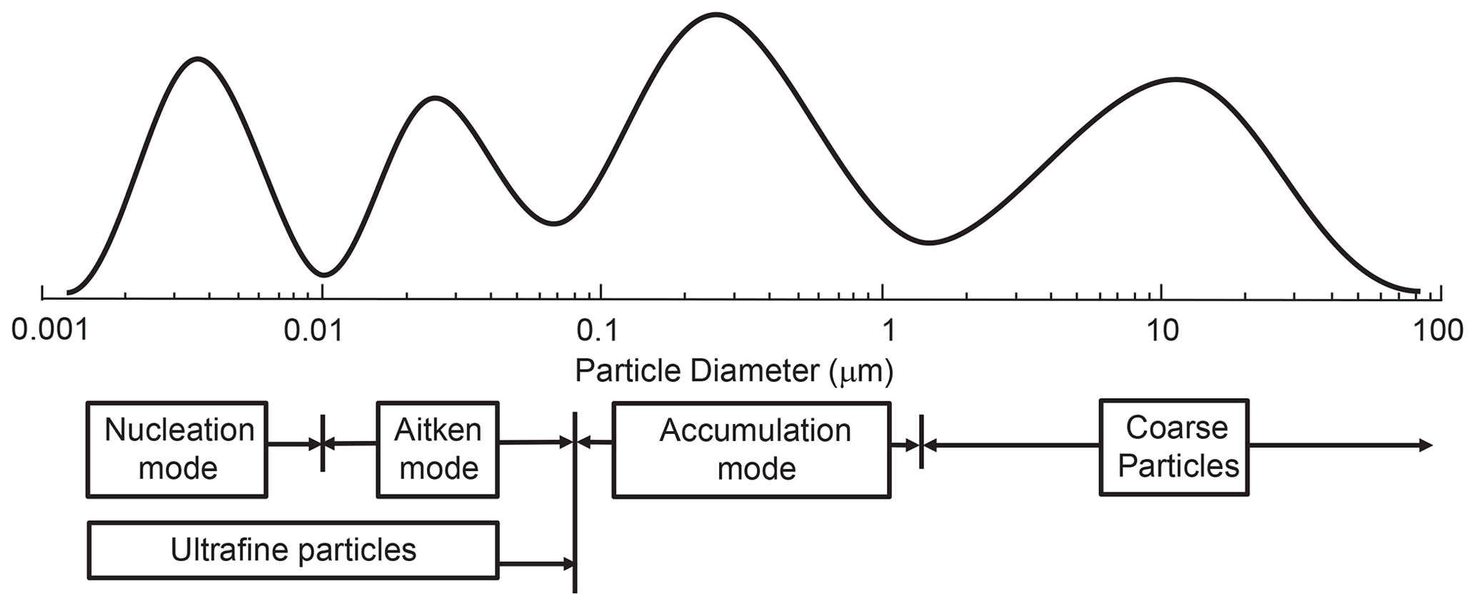
Figure 1 An example of a particle size distribution consisting of a number of different modes. The names of the different modes and sizes are shown.

By definition, an aerosol consists of particles or droplets suspended in a gas phase of varying complexity. Aerosol particles, both natural and anthropogenic, are either directly emitted or formed in situ in the atmosphere through gas-to-particle conversion (nucleation). Furthermore, aerosol particles are highly variable in size, from nanometres to micrometres in diameter. The majority of the particle number concentration appears in the ultrafine size range below 100 nm (often divided into the nucleation mode with diameters up to 10 nm and the Aitken mode for those about 10 to 100 nm in diameter). The surface area and the mass concentration are often highest in the size range of the accumulation mode, typically between 100 nm and 1 µm in diameter. However depending on location and season, a substantial part of the aerosol mass and surface can be found in the coarse mode. Coarse-mode particles typically have a short lifetime in the atmosphere due to their rapid settling velocity. Particles larger than the accumulation mode are denoted as the coarse mode (see naming conventions in Fig. 1). The PNSD, chemical composition and hygroscopicity are critical parameters determining the fate of the particles during transport in the atmosphere. These are closely linked to key processes such as condensation, coagulation, and dry and wet deposition including the potential to act as cloud condensation nuclei (CCN).

Condensation of low-volatile gas-phase species and evaporation from the surface of the particles are continuous mechanisms that affect the size of the aerosols and the chemical composition. Coagulation, when particles agglomerate to form larger particles, reduces the number concentration of the particles and transforms the size distribution while conserving the mass of the species within the aerosol.

Aerosol particles are removed from the atmosphere by dry and wet deposition. Dry-deposition efficiency is strongly size dependent, and ultrafine particles and supermicron particles have comparably short lifetimes compared to accumulation-mode aerosol.

The high deposition velocity due to Brownian motion is most effective on particles smaller than 50 nm, resulting in a comparably high deposition velocity. Supermicron particles in the coarse mode (Fig. 1) have a relatively short lifetime (high deposition velocity), due to gravitational settling and inertial impaction. The accumulation mode, representing the size range of aerosols with the longest lifetime in the atmosphere and thus how rapidly a trace substance enters the accumulation mode through either condensation or coagulation, is of crucial importance for the atmospheric lifetime of the trace substance in the atmosphere.

Coagulation, condensation, chemical interactions with surrounding gases and hygroscopic growth determine the composition of atmospheric aerosols. The size and chemistry of aerosol determines cloud-forming potential (acting as CCN) and thus efficiency of wet removal. Wet removal through in-cloud and below-cloud scavenging is the most important sink for atmospheric aerosols. There are many good sources for in-depth information concerning aerosol physiochemical processes and atmospheric aerosols (e.g. Seinfeld and Pandis, 2006).

The deposition field, defined as the amount and spatial distribution of particles deposited to the surface, determines the external dose to people and the environment. When particles deposit, they act as a sink for the air concentration as well as a “source” for the deposition field. In radiological emergency preparedness both the deposition field and the remaining air concentration are of importance for calculating the external dose and inhaled internal dose.

Ideally, all atmospheric aerosol processes should be considered in dispersion models. Due to computational limitations and the complexity of physical parameterizations, dispersion models for emergency preparedness have been developed based on simplified physics. When it comes to Lagrangian particle dispersion models (LPDMs) that rely on the transport of discrete model particles, only first-order processes can be applied with computational ease. The rate by which coagulation, condensation, dry deposition, cloud formation, precipitation and wet deposition affect the aerosol particle population depends on the dynamic process considered in the air parcel. Traditionally, the aerosol dynamic is not simulated in LPDMs to this extent. Examples of LPDMs are the open-source model FLEXPART (FLEXible PARTicle dispersion model; Stohl et al., 1998; Pisso et al., 2019), the UK Met Office dispersion model NAME (Numerical Atmospheric-dispersion Modelling Environment; Jones et al., 2007) or the NOAA HYSPLIT (Hybrid Single-Particle Lagrangian Integrated Trajectory) model (Stein et al., 2015). They all have different parametrizations for wet and dry deposition. The released model particles in an LPDM usually remain in the same size class as prescribed by the sources function for the full duration of the simulation or until they are lost through deposition processes. Treating the model particles as discrete entities without any interaction with the surrounding aerosol particle population introduces errors in the simulations of both dry- and wet-deposition processes, which are strongly dependent on the PNSD and abundance of both scavenged and surrounding aerosol particles. This treatment further neglects condensational growth and coagulation for a size where they can act as CCN and be available for in-cloud scavenging. Therefore, the total wet deposition could be underestimated substantially, as there are no dynamic feedbacks on the aerosol–cloud interaction.

This dynamic feedback can be viewed from two different angles, linking to competitive growth during cloud formation on the one hand and condensation growth on the other hand. As wet deposition to a substantial degree occurs through nucleation scavenging, parts of the available CCN are removed. If the PNSD remains static, a second cloud cycle will tend to result in activation starting at a lower size range; i.e. the activation and subsequent removal “eats” its way through the distribution, taking chunks away from right to left with an increasingly lower activation radius as a result. This will make smaller and smaller particles available for in-cloud scavenging and removal. Now, if the activation diameter instead would be fixed and for simplicity assuming it to be 100 nm, once all 100 nm particles are removed no more in-cloud scavenging can occur. This of course is unrealistic, as it is well established that activation is controlled by competitive growth and that the lower the number of large particles is, the smaller the activation radius resulting for a given set of conditions will be. Hence, the cloud activation radius and removal will be adjusted based on the previous removal events. The second link is when particles are grown due to condensation growth (and to lesser extent coagulation). These processes bring particles that otherwise would be too small to be activated into a size range where they in fact may become actual CCN. Studying this dynamical coupling (or feedback) between growth, removal and cloud droplet activation is one of the main targets of this study.

There are Eulerian methods of dispersion modelling which have a more advanced take on aerosol dynamics; for example WRF-Chem (Weather Research and Forecasting model coupled with Chemistry; Grell et al., 2005) has an optional aerosol module simulating aerosol nucleation, condensation and coagulation. WRF-Chem is an online model where aerosol microphysical processes are simulated within the meteorological model itself. Simulating aerosol dynamics on a regional to global scale is also done in general circulation models (e.g. Vignati et al., 2004), chemical transport models (e.g. Spracklen et al., 2005) and air quality models (e.g. Zhang et al., 1999). There are examples of Eulerian–Lagrangian hybrid models, for example in Danielache et al. (2019), where the Eulerian part calculated the chemical transformation and the Lagrangian was used for transport. For emergency preparedness fast models are essential. To our knowledge there has been no solution presented providing sufficiently fast and detailed aerosol dynamic representations within the strictly Lagrangian framework applied in LPDMs used for dispersion simulations of radionuclides in a Fukushima type of accident; dispersion of emitted ¹³⁷Cs is of major concern, since it is one of the isotopes giving long-term complications, and ¹³⁷Cs is therefore continuously monitored around the globe (IAEA, 2010). A release of vaporized ¹³⁷Cs condenses on the surface of the surrounding aerosol particles, giving it an activity size distribution largely following the surface area size distribution of that carrier aerosol. In an LPDM, the dispersion of the aerosol is simulated by transporting model particles that each represent a part of the source. Henceforth, the individual particles will only undergo first-order dynamics (i.e. highly parameterized wet removal, dry deposition and radioactive decay). Neither the PNSD nor the chemical composition of the advected particle will change in the classic way in which LPDM simulations are performed. This potentially poses a significant problem. As previously described, removal through wet deposition is highly dependent on both the PNSD and the chemical composition of the aerosol particles. Without altering processes of the particle population, the simulation is prone to the risk of either overestimating or underestimating the removal depending on the initial conditions prescribed at the release point.

In this study, a Lagrangian trajectory model, Chemical and Aerosol Lagrangian Model (CALM; Tunved et al., 2010), was used. CALM simulates the evolution of the physical and chemical properties of an aerosol following an air mass trajectory. The air mass trajectories are calculated using meteorology from a numerical weather prediction model to describe the path of the trajectory and its meteorological properties. CALM calculates the transformation of the PNSD and associated size-resolved chemical composition due to nucleation, coagulation, condensational growth, dry and wet deposition, chemical transformation, and new sources along the trajectory. In this study, CALM has been modified (from a coupled two-box model, simulating the mixing layer and the residual layer) into tracking one box forward in time that moves also in height above the ground in and out of the mixing layer (depending on the current trajectory). In this way, the used model setup does not simulate a single particle or a static number size distribution, i.e. the most commonly used designs in classical LPDM models. Instead we allow the simulated trajectories to carry a complete PNSD that will age and transform during transport. Simulations have been done for different sites and under different meteorological conditions to account for the variations that can occur due to different weather conditions, different air masses and new aerosol sources along the path. They have all been initialized with a measured PNSD unique for that time and location. One should bear in mind that the purpose of this study is not to calculate atmospheric dispersion (the single-trajectory approach is not suited for dispersion calculations) but rather to study the potential impact resulting from omission of a detailed aerosol dynamic treatment, including the activation into cloud droplets, in current LPDM frameworks.

In this experiment however, the wet-deposition scheme is more advanced than in many LPDMs using a scavenging coefficient. It includes below-cloud scavenging and in-cloud scavenging with CCN activation based on updraughts and atmospheric lifetime and deposition efficiency of radioactive material compared to the standard way currently adopted in LPDMs, i.e. treating deposition as a first-order process only.

The purpose of the study is to investigate the following:

• When is a more sophisticated aerosol dynamic treatment in LPDM simulations needed?

• Is the current treatment of aerosol removal processes in LPDMs sufficient for the simulation used in radiological emergency preparedness?

• Which aerosol dynamic and cloud processes are most crucial to include in LPDMs to improve their accuracy?

• How do geography-specific and seasonal characteristics of meteorology and source profiles influence the atmospheric lifetime of radionuclides emitted from an intermittent point source?

2 Method

To examine the impact of aerosol dynamics in an LPDM framework, the Lagrangian trajectory model CALM was used (Tunved et al., 2010). Using CALM, the evolution of an aerosol was simulated along a large set of air parcel trajectories originating from three different measurement stations in Europe.

A full year of PNSD measurements of the ambient aerosol at each of the three stations initiated the model for each individual simulation. Different modelling experiments were performed for all the trajectories to investigate the impact of simulating different processes.

2.1 Trajectory calculations

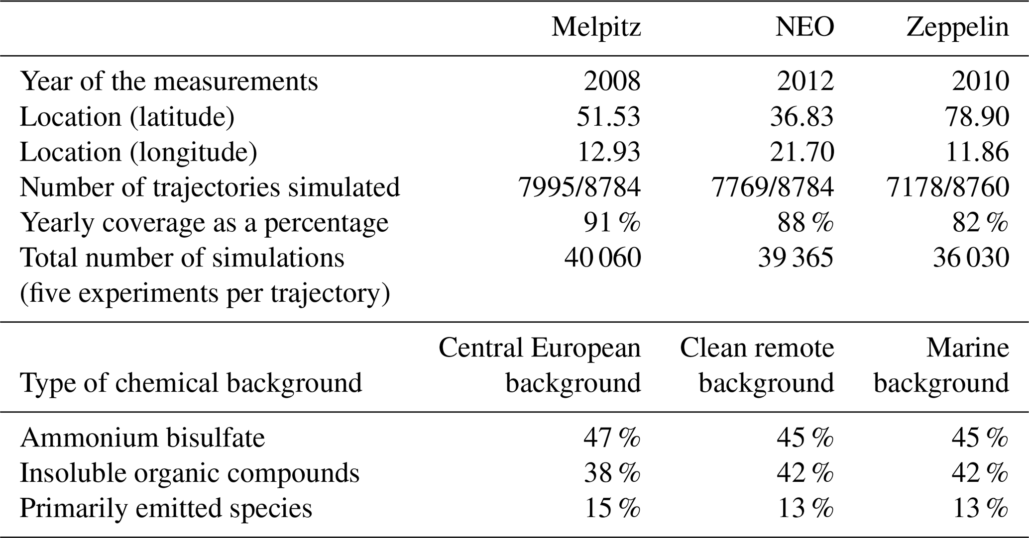
By simulating 24 different trajectories each day (one for each hour) the variability of the ambient PNSD, in the meteorology and in the transport paths could be analysed. An air mass forward trajectory by definition describes the advection of an infinitesimal particle and can be used to describe the transport of a released substance or an air parcel. The three-dimensional (latitude, longitude and height) trajectories used in this study were calculated with the HYSPLIT model in forward mode (Stein et al., 2015) using fields from the meteorological model GDAS (Global Data Assimilation System; NOAA, 2019) with a geographical resolution of 1^∘ in latitude and longitude and temporal resolution of 3 h. From these calculations, both the trajectory path (based on three-dimensional mean winds) and important meteorological parameters along the path were retrieved and used as input for CALM. In each individual simulation, CALM was run along the air mass trajectory for the duration of 10 d. In theory, there would be $\mathrm{365}\times \mathrm{24}=\mathrm{8760}$ trajectories to analyse for each station for a full year (that is not a leap year), but due to missing data in the measurement series the actual number of trajectories is somewhat lower (see statistics in Table 1).

Table 1 Stations for the simulations, data and initial chemical conditions.

2.2 Measurement stations and aerosol data

The three chosen stations represent climatologically different regions, and the trajectories from the stations travelled through different types of terrain. The ambient-aerosol measurements at the stations were then used to initiate the CALM model. As the trajectories are calculated using re-analysed data, simulated travelled paths and associated meteorology will vary following seasonality and climatological characteristics in different environments as well as exposure to different source patterns. Together with the seasonal variability of the ambient PNSD, the simulations will cover a wide range of characteristics, which will provide the basis for the evaluation of the impact of various processes affecting deposition fields and residence time of radionuclides attached to the aerosol phase.

The measurement station in Melpitz (TROPOS, 2020) in the centre of Europe was chosen as a representation of the central European background with transport patterns mainly from eastern and western Europe. NEO (Navarino Environmental Observatory) in Greece (APCG, 2020) represents a coastal area where the ambient aerosol is strongly influenced by local sources by the coast and long-range transport, in this case from northern Italy and the Balkans, occasionally with Saharan dust. The forward air mass trajectories starting at NEO often travel over the Mediterranean Sea. Zeppelin in the polar region (Norwegian Polar Institute, 2020) represents a remote background station with both natural sources and long-range transport from anthropogenic sources. At Zeppelin, the ambient background has a substantially lower particle number concentration than the other two stations. The location of the three stations can be seen in Fig. 2.

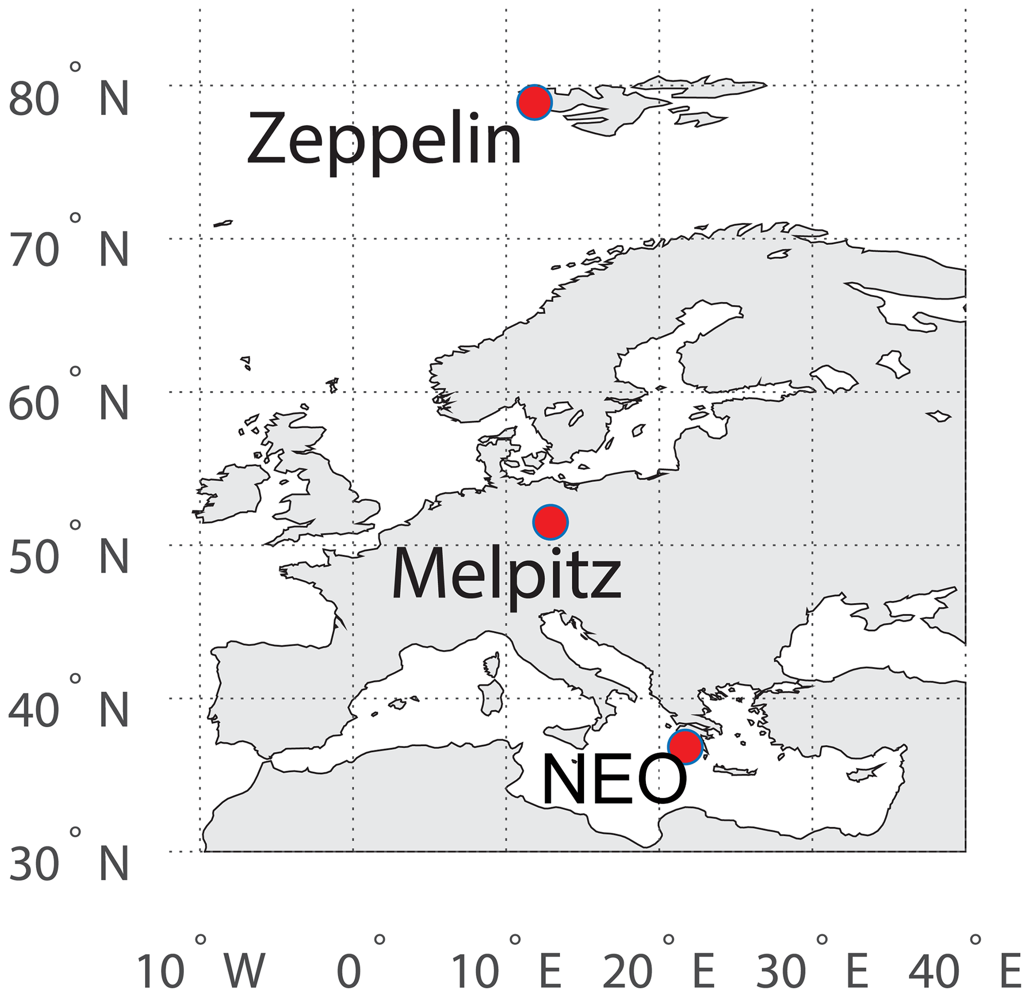
Figure 2 Measurement stations. The particle number size distribution (PNSD) measured at the stations are used to initiate the trajectory calculations.

The measurement time series should have as small gaps as possible for the chosen years (which should be near each other not to involve climatological differences). This made us chose different years for each station, still representing seasonal variability for the analysis. For Melpitz the year 2008 was chosen, where 7995 out of the year's 8784 h had measurements (91 % coverage) (Reddington et al., 2011); for NEO the year 2012 had 7769 out of 8784 h (88 % coverage); and for Zeppelin 2010 was chosen with 7178 out of 8760 h (82 % coverage) (Tunved et al., 2013). For Zeppelin we have omitted the month of December, since there were too few individual trajectories to analyse (based on the availability of measured size distribution).

All three stations observe the PNSD using similar setups of different kinds of mobility particle size spectrometers (MPSSs). Sizes covered by the instruments range from a couple of nanometres up to several hundred nanometres. The supermicron size range is however not included in this study. Doing so, we are aware that the omission of the coarse mode potentially could introduce significant deviation from current results. This is especially true for occasions where the surface area is completely dominated by supermicron particles. Being prone to rapid dry deposition through sedimentation, similar situations could result in comparably fast removal of attached radionuclides.

Information about the instrumental setup can be found in e.g. Tunved et al. (2013) for the Zeppelin site and Birmili et al. (1999) for the Melpitz site. PNSD observations at NEO are pending publication. The stations are part of the European Research Infrastructure ACTRIS (Aerosol, Clouds and Trace Gases Research Infrastructure), in which the measurements and the quality assurance and control are harmonized (Wiedensohler et al., 2012, 2018).

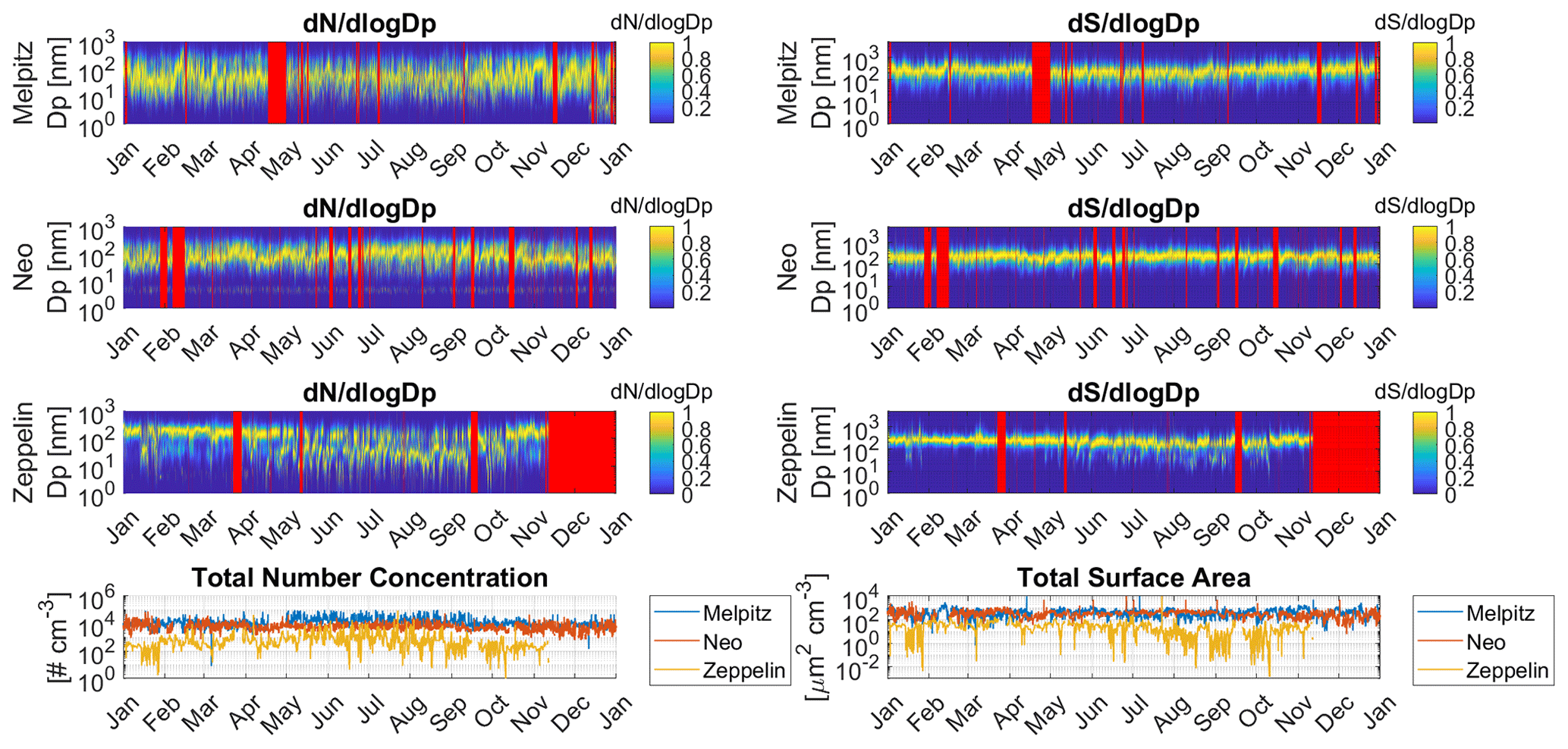
Figure 3 Seasonal development of the initial PNSD normalized to the maximum in the bin with the highest concentration (left column) and initial surface size distribution normalized to the maximum in the bin with the largest surface area (right column). Melpitz in 2008 (top row), NEO in 2010 (second row) and Zeppelin in 2012 (third row). Three modal fits calculated from measurements at each station. The bottom row contains the total number concentration (left) and total surface area (right).

In order to harmonize the data into a format that directly can be input to the model, each hourly PNSD was fitted under the assumption that each PNSD can be represented by three log-normally distributed modes. Each mode is defined by a number concentration (N), a geometrical mean modal diameter (Dg) and a geometric standard deviation (GSD) that defines the spread of N around Dg for each mode. See Fig. 3 for the PNSD (left) and surface size distribution (right) for the three stations. The total number concentration and total surface area are in the bottom row. The best fit was found through solving a constrained minimization problem that gives the optimal distribution into three distinct log-normal modes under the constraint of non-negative weights. In a few cases (0.6 %) the automatic fitting process did not work, and these occasions were not simulated. Seasonal variations in the PNSD can be noticed for all stations, where Zeppelin stands out (cf. Fig. 3). PNSD seasonality in the Arctic is driven by local sources, remote sources and transport patterns as well as differences in precipitation patterns (Tunved et al., 2013). The total concentration of particles is lower in the Arctic than for the other station, which makes it more sensitive for variations. The spring period, February to April, consists of an aged and elevated accumulation-mode aerosol strongly influenced by remote sources linked to meteorological transport patterns and inversions trapping the aerosol and reducing dilution. This is commonly referred to as Arctic haze. The number concentration during the summer period, May–September, is formed through mainly gas-to-particle conversion resulting in a pronounced Aitken mode towards as well as intermittent presence of a nucleation mode (cf. Fig. 2). Since particle formation is dependent of sunlight, there are also strong diurnal variations in this period.

The aerosol particles are assumed to be internally mixed; i.e. all aerosol particles of a certain size have the same chemical composition (as opposed to being externally mixed, where one size class can contain particles of various compositions). CALM divides the internal mix of the particles into three different chemical groups, ammonium bisulfate, condensable and partially water-soluble organic compounds, and primarily emitted species. The setup assumes irreversible condensation of ammonium bisulfate and organic material, and no chemical reactions take place in the dry particle phase (although wet-phase oxidation of sulfur dioxide in cloud droplets is considered when present). In the current setup we have added a third condensable species with saturation vapour pressure set to zero to replicate intermittent irreversible condensation of ¹³⁷Cs on the size distribution. The initial aerosol chemical composition comes from a general description in Putaud et al. (2004) where their definitions of a “Near-city & urban” composition has been used to represent the central European background for Melpitz and their definition of a “Natural & rural” composition has been used for representing the clean remote background for Zeppelin and the marine background for NEO, respectively (see composition in Table 1). Chemical transformation of the particles has not been studied, and this crude generalization was considered sufficient for this study.

2.3 Radioactive particles

Our topic of interest is the dispersion of radioactive particles from a failure of a nuclear power plant; ¹³⁷Cs is monitored all around the globe for radiological preparedness, since it is one of the isotopes causing most of the long-term damage. For this study, we assume that all released ¹³⁷Cs from a failure of a nuclear power plant is attached to the ambient aerosol in the vicinity of the power plant, as assumed in the study by Kristiansen et al. (2016). This assumption will serve the purpose for this study, even though particles containing ¹³⁷Cs internally (not only on the surface) have been found after the Fukushima accident (Adachi et al., 2013; Higaki et al., 2017). The caesium is present in small enough quantities not to affect the aerosol dynamics in the model but instead used as an inert tracer. In this context, the unit of Cs is arbitrary, but we will refer to it as Becquerel throughout the paper. Throughout the simulation, the distribution of ¹³⁷Cs and ambient aerosol, respectively, was traced, showing the effect of the aerosol dynamic processes.

In the experiments with CALM, the release of ¹³⁷Cs had a duration of 800 s and started 60 min into the simulation. The ¹³⁷Cs was released as a gas, and the concentration for saturation above a flat surface was set to zero to make it condense irreversibly on the surface of the particles present in the ambient aerosol. Throughout the simulation the distribution of ¹³⁷Cs and the number distribution of the whole aerosol could be traced, respectively, showing the effect of the aerosol dynamic processes.

2.4 Model setup

CALM describes the evolution of the PNSD as well as the ¹³⁷Cs activity distribution. The aerosol dynamic processes of condensational growth, coagulation, nucleation of new particles, new sources, wet deposition and dry deposition were turned on or off in different experiments to analyse their individual impact.

The dry deposition includes Brownian diffusion, most effective for particles smaller than 50 nm, and gravitational settling and inertial impaction, which is most effective for particles larger than a few micrometres in size. Dry deposition in the model setup is only active when the box is in the mixing layer and when particles can reach the ground. This neglects the effect of gravitational settling for particles above the mixing layer, and this effect can be large when aerosol surface is dominated by coarse-mode particles.

The model design utilizes a hybrid approach and considers two different compartments: one for ambient-aerosol dynamics and one for aerosol–cloud interactions and in-cloud scavenging. The dry “ambient-dynamic” box considers detailed descriptions of gas-to-particle conversion, dry deposition and coagulation. Decoupled from this box we run an adiabatic one-dimensional cloud module that calculates activation and growth of aerosol particles in an ascending air parcel. The cloud model is run separately from the ambient-dynamic box when clouds are prescribed. The cloud compartment results in a droplet distribution of the activated particles, which in turn allows us to calculate a liquid water content (LWC). The environmental parameters framing the cloud calculations are based on meteorological parameters provided by the meteorological model (GDAS) which are calculated every 3 h. Exactly how this is done is outlined below. Once formed, available SO₂ is equilibrated to the bulk water together with ozone and hydrogen peroxide. This allows for calculation of pH and concentration-dependent liquid-phase oxidation of sulfur dioxide. This means that if the cloud does not precipitate, the sulfate produced through this pathway is distributed over the activated particles. This means that the cloud does in fact have the potential to act as a source of aerosol mass.

Apparently, there is a discontinuity comparing on the one hand the cloud and on the other hand the ambient box. We have chosen this approach, since we want to retain the key processes of activation and its link to aerosol size distribution properties and chemistry. Once the cloud dissipates, the effect it has had on the aerosol in the ambient-dynamic box (in-cloud chemistry and in-cloud scavenging) is evaluated based on the fraction of the box that has been influenced by the cloud, which is determined from humidity profiles and fractional cloud cover.

Concerning wet deposition, the process when the aerosol particles act as cloud condensation nuclei and initiate a cloud droplet is called activation. CALM utilizes a zero-dimensional activation scheme, where the activation and growth are explicitly calculated in an ascending air parcel at prescribed but variable updraughts. This determines the smallest size of the activated particles at each instance of cloud formation. Clouds are considered every 3 h; the model calculates a vertical profile of pressure, temperature and humidity as well as the fraction of low, midlevel and high clouds. If clouds are present in the vertical column, the model checks if the humidity at the altitude coincides with that of the air parcel. The vertical resolution of the meteorological model used (GDAS, 1^∘) is, starting from the bottom going up, at 1000 hPa with 25 hPa resolution up to 900 hPa and 50 hPa resolution up to levels relevant for the current simulations. The vertical resolution is 1^∘. If the humidity is above 99 %, the vertical extent of cloud is estimated as the total number of adjacent levels with the RH (relative humidity) above the threshold. The cloud fraction from the meteorological model is then used to scale how big of a fraction of the air parcel is subjected to cloud activation, in-cloud chemistry and eventually removal. Thus, if the model suggests 50 % cloudiness and if the air parcel is at an altitude where the RH is above the threshold, 50 % of the aerosol is involved in the activation, and the rest remains as is. Likewise, if the model indicates precipitation (given as precipitation at ground level (mm h⁻¹) representing the all precipitation from the column above the ground), only 50 % is affected by wet removal. The fraction removed per millimetre of precipitation is scaled to the calculated liquid water path (LWP) (g m⁻²) and column precipitation intensity. If cloudiness is 100 %, 100 % of the aerosol is subjected to activation and removal processes. This does however not automatically mean that 100 % is removed. If the cloud is thick and of high LWP and the precipitation rate is low, this will result in low scavenging rates in the air parcel. The in-cloud scavenging scheme further assumes warm clouds (i.e. without an ice component). In-cloud scavenging is subsequently calculated from a modelled precipitation rate, assuming growth into precipitation-sized droplets occurs via collision coalescence between cloud droplets in the cloud. The effect of ice components in clouds is neglected, which may alter the scavenging efficiency and ultimately the wet-removal rate. Clouds are prescribed when relative humidity of the parcel is above 99 %, a condition that initiates calculation of the cloud with a randomly chosen constant updraught between 0.1 and 1 m s⁻¹, with a normal distribution around 0.5 m s⁻¹, representing a typical stratocumulus cloud. Admittedly, being of crucial importance for the lower size limit of activation, this approach has limitations, e.g. the crude assumption of the randomized updraughts, and it is not valid for convective precipitation or subgrid-scaled clouds. Nevertheless, we argue that the range of updraughts used reflects different cloud conditions ranging from typical low-level stratus up to shallow convective clouds. The box tracked along the trajectory is either below, in or above a cloud if there is a cloud in the column where the box is situated. If the box is in the cloud, it is subject to calculation of droplet activation in-cloud scavenging, if it is below sub-cloud scavenging. The in-cloud scavenging washes out only a fraction of the activated particles. This fraction is a function of the cloud water content (calculated from the liquid water path for the cloud) and ground level precipitation (which are parameters available in the meteorological fields used to calculate the trajectory). The below-cloud scavenging uses a parameterization by Laakso et al. (2003).

The difference between modelling wet deposition in CALM (a trajectory box model) and what is commonly used in an LPDM model is quite substantial. In CALM the removal dynamics are made to mimic what happens in a real cloud which traditionally has been too computationally heavy for inclusion in an LPDM. Traditionally in an LPDM, a scavenging coefficient that depends on meteorological parameters is used (Sportisse, 2007). The scavenging coefficients used for both in-cloud scavenging and below-cloud scavenging are often empirically determined. This inevitably creates a bias of the scavenging coefficients towards conditions typical for the chosen experiments and might thus not represent the variety of wet deposition that takes place in reality. For this reason alone it would be desirable to include more advanced wet-deposition modelling in dispersion models.

To simulate something that an LPDM dispersion model could afford computationally, a simplified version of the activation scheme was used with a fixed CCN activation size instead of one calculated from updraughts and humidity. This will henceforth be denoted fixed activation size (FAS) in the experiment description.

Table 2 The different experiments.

2.5 The different experiments

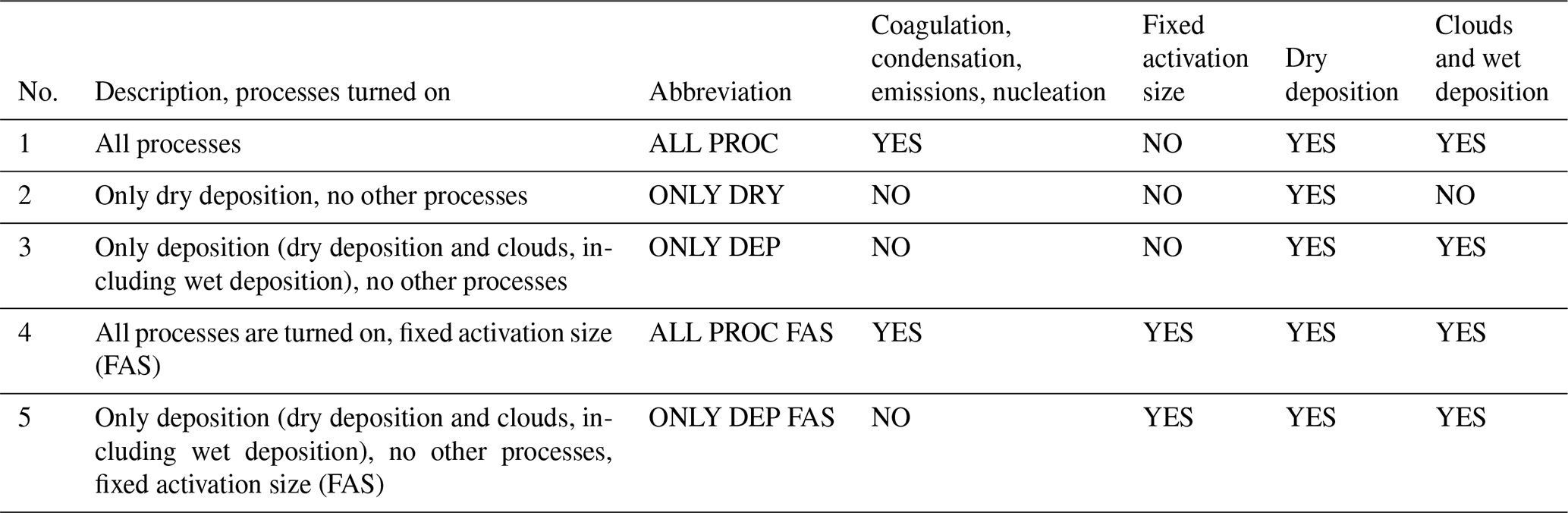
For each of the trajectories we made five different experiments simulating single trajectories to analyse the impact of aerosol dynamics, summarized in Table 2. The experiments were designed in a way to, as transparently as possible, evaluate to what degree simulating advanced aerosol dynamics in LPDMs could influence the overall result. Identifying where and when detailed treatment could be beneficial is important in the context of emergency preparedness after an accident at a nuclear power plant:

1. In the first experiment (abbreviated ALL PROC), we used the full setup with all aerosol dynamics including wet and dry deposition. This simulation represents the most detailed description of what a single trajectory of an LPDM dispersion model run would give as a result if it were to simulate all aerosol dynamic processes. Comparison with this experiment will show the effects of omitting certain processes.

2. In the second experiment (abbreviated ONLY DRY), only dry deposition was active (no wet deposition and no other processes). This simulation represents the behaviour in the dry atmosphere without other aerosol dynamics. This is the simplest single-trajectory setup representing a dispersion model mimicking either behaviour when there is no ongoing precipitation or a model omitting wet deposition totally. It will give us a sensitivity analysis of the behaviour in the dry atmosphere if we were to neglect simulating all other processes.

3. The third experiment (abbreviated ONLY DEP) simulated dry deposition and clouds (including in-cloud and below-cloud scavenging) but no other aerosol dynamics. This is an analogue to the common approach in dispersion modelling where only wet and dry deposition are simulated. In this experiment however, the wet-deposition scheme is more advanced than in many LPDMs using a scavenging coefficient. It includes below-cloud scavenging and in-cloud scavenging with CCN activation based on updraughts and available humidity (henceforth denoted advanced wet-deposition scheme or advanced cloud parameterization). This experiment represents the behaviour of an LPDM with an advanced wet-deposition scheme.

4. The fourth experiment (abbreviated ALL PROC FAS) is similar to the first experiment with all processes turned on but with a fixed CCN activation size (FAS) resulting in a simplified wet-deposition scheme. This experiment represents the behaviour of a dispersion model with a simplified wet-deposition scheme but where the coagulation, condensation, emissions, chemical transformations and nucleation (henceforth denoted advanced aerosol dynamics) are included.

5. The fifth experiment (abbreviated ONLY DEP FAS) included dry deposition and wet deposition with the fixed activation size but no other processes. This experiment mimics the traditional LPDM without advanced aerosol dynamics and with a simplified activation scheme (which still has a more advanced wet-deposition scheme than the traditional scavenging coefficient approach often used in dispersion models).

Note that including cloud interaction with a fixed activation size (FAS) as in experiments 4 and 5 is still a more advanced approach than the wet scavenging commonly used in LPDMs.

3 Results

The outcome of the trajectory simulations described above is presented in this section. We have calculated “average trajectories” by combining the output of each individual time step counting from the start of the simulations. This was calculated into annual and monthly “average trajectories” with particle and caesium concentration throughout the 10 d simulations for each of the sites. Normalized Becquerel values represent ¹³⁷Cs where 1 denotes all released ¹³⁷Cs and 0.1 denotes 10 % of the released amount.

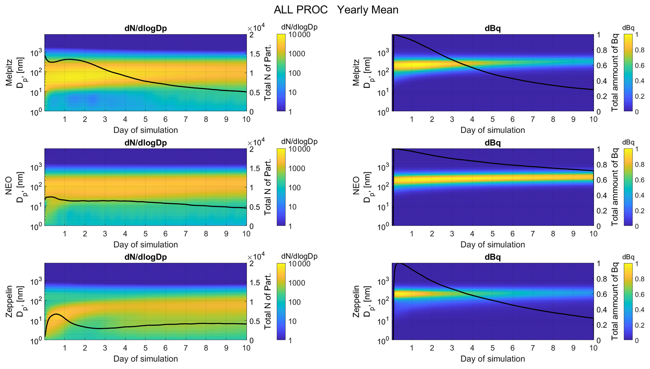
Figure 4 Evolution of the PNSD, $\text{d}N/\text{d}\log D_{\text{p}}$ (left column) and Becquerel size distribution (right column) for the experiment when all processes are turned on (ALL PROC, annual mean). Black lines are the total number of particles and the total amount of ¹³⁷Cs in the respective graph (right-hand axes). Calculations from Melpitz, NEO and Zeppelin in the top, middle and bottom row, respectively.

The evolution of the ambient PNSD of the aerosol and the size distribution of released ¹³⁷Cs (activity size distribution of the ¹³⁷Cs attached on the particles) is shown in Fig. 4. This plot shows the annual mean average of the first experiment where all processes are turned on, ALL PROC; ¹³⁷Cs is represented as a Becquerel value normalized to the maximum value. The total particle number concentration and the total amount of ¹³⁷Cs attached on the particles are plotted as black lines in respective graphs (right-hand axes). The rows show Melpitz, NEO and Zeppelin, respectively, with $\text{d}N/\text{d}\log D_{\text{p}}$ to the left and ¹³⁷Cs (Becquerel values) to the right. The development over the 10 d period is an effect of different routes of the individual trajectories, meteorological conditions, new sources and aerosol processes along the path. Even though each track has its individual characteristics and events, annual and monthly averages show features representative for each site and period. The radioactive caesium is released 1 h into each simulation and condensates on currently available particles to be mixed with “clean” particles from new sources along the path.

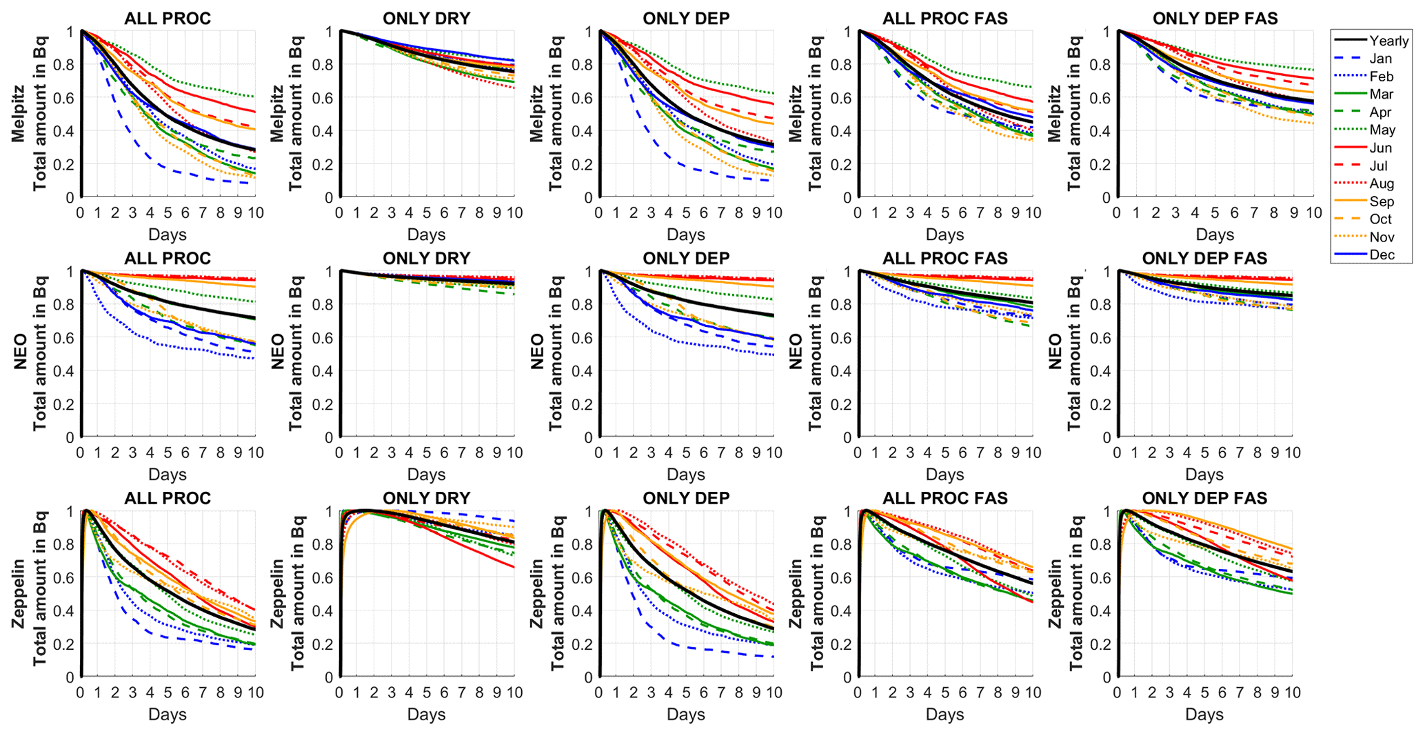
Figure 5 Annual (black) and monthly means (blue for winter, December–February; green for spring, March–May; red for summer, June–August; and orange for autumn, September–November). Development of caesium concentration as normalized Becquerel values for the five different experiments. Each row represents a different station (from the top, Melpitz, NEO and Zeppelin), and the columns are the different experiments, ALL PROC, ONLY DRY, ONLY DEP, ALL PROC FAS and ONLY DEP FAS.

For Melpitz, the average PNSD decreases after an initial peak 1 d into the simulation. The peak in the PNSD moves slightly towards larger particles throughout the 10 d period. There is a very small but continuous increase in small particles (< 10 nm) after the first day, throughout the simulation. The PNSD for NEO has a two-modal initial distribution with many small particles (smaller than 10 nm). The total particle number concentration decreases after a small peak half a day into the simulation. After 2 d of simulation, the change in $\text{d}N/\text{d}\log D_{\text{p}}$ is barely visible even though the total particle number concentration decreases slightly. The PNSD in Zeppelin shows that it starts with a peak for particles smaller than 10 nm that grows in both size and number during the first 12 h. After that the total particle number concentration decreases until late in day 2 where it starts growing slightly during the continuation of the simulations. The peak of the PNSD grows for Zeppelin throughout the whole simulation from around 10 nm to almost 100 nm.

The change in total ¹³⁷Cs activity can be seen in Fig. 5 for the five different experiments (see Table 2), represented by normalized Becquerel values (from 0 to 1). Each row represents one of the three stations, and the columns represent the different experiments. The black line in each plot is the evolution of the annual mean, while monthly means are the lines with different colours. The December monthly mean has been omitted for the Zeppelin cases, since it had only 6 out of 744 possible simulations (0.9 %), which was considered to be too few for statistical calculations.

The first column shows the experiment when all aerosol dynamic processes are turned on (ALL PROC). The different stations have different characteristics. The variability of monthly means at the end of the 10 d period is greatest for Melpitz (a spread of 52 percentage points) and smallest for Zeppelin (a spread of 24 percentage points) even though Zeppelin has a greater variability after 4 d (a spread of 50 percentage points). NEO has a difference of 48 % at the end of the simulations. The summer months for NEO have a small decrease in caesium concentration. NEO has the smallest decrease of all the stations, down to 70 % of the original amount compared to 28 % for Zeppelin and 27 % for Melpitz. Melpitz has for all months a faster decrease in the first half of the simulation than in the second half. This is also true for the winter months in Zeppelin but not for summer and autumn.

The ONLY DRY experiment, in the second column, has only dry deposition turned on, i.e. no wet deposition and no other aerosol dynamic processes. The differences between the stations is due to the difference in the initial aerosol size distribution spectra and its dry deposition along the trajectories. Dry deposition only occurs when the box is in the mixing layer, so the height variation of the box also plays a role. The variation in monthly means after 10 d is greatest for Zeppelin (a spread of 27 percentage points) and smaller for NEO (a spread of 10 percentage points) and Melpitz (a spread of 16 percentage points). The total decrease for the annual mean was for Zeppelin down to 80 % and 75 % for Melpitz; NEO had the smallest decrease to 92 % of the released amount.

ONLY DEP, the experiment in the middle column, includes both dry deposition and advanced cloud parameterization with wet deposition but no other aerosol processes. The difference between this experiment and the previous one comes from the effect of wet deposition. This result is similar to the first experiment, ALL PROC, where all processes are taken into account. Both share the same advanced cloud-processing scheme.

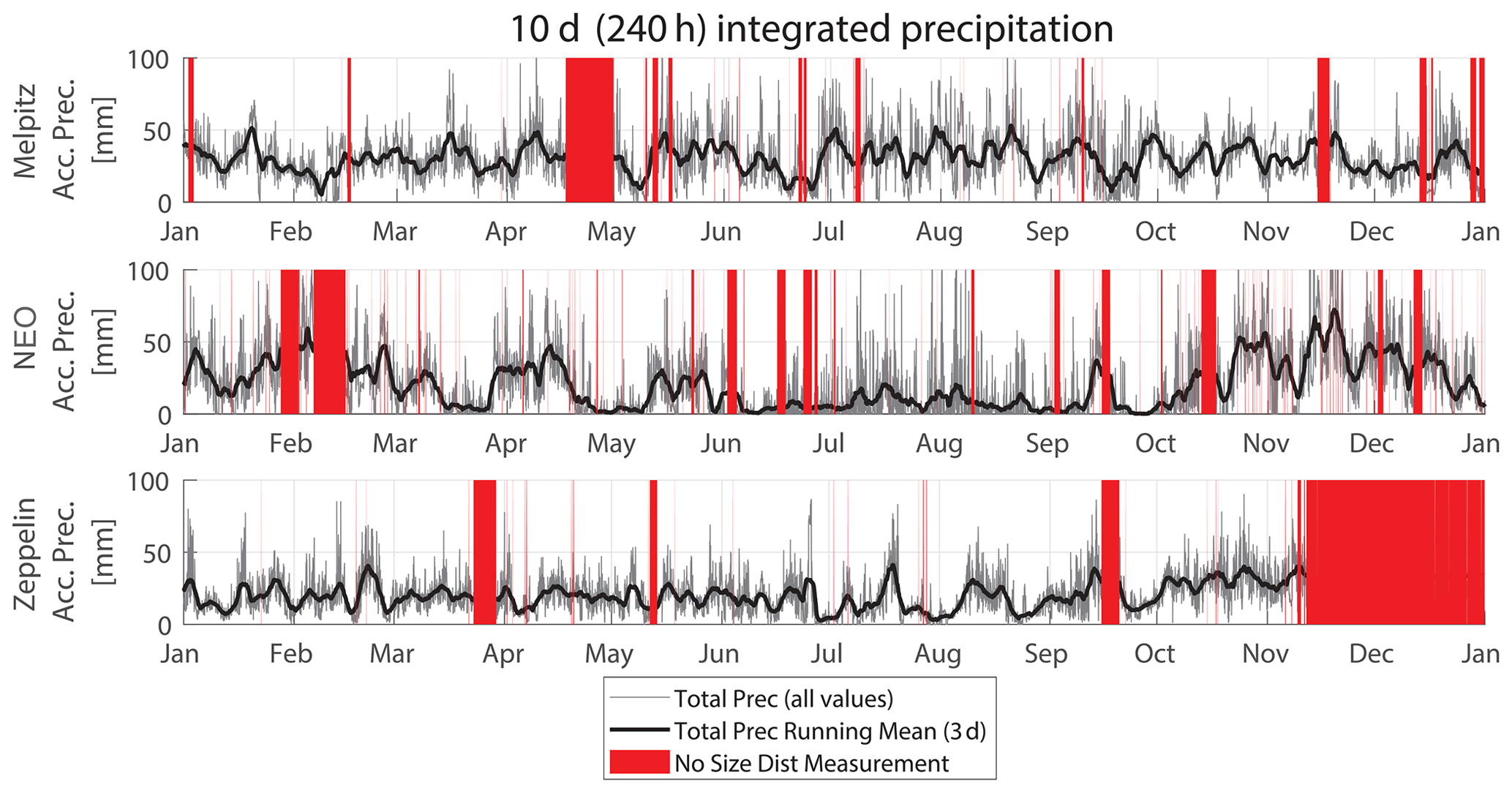
Figure 6 Total accumulated precipitation (Acc. Prec.) for each 10 d trajectory for the three stations (grey line). The black line is a moving 3 d mean, and red areas are periods with no input data (no size distribution (Dist) measurement and hence no simulations). The y axis is set to 0–100 mm even though there are a few peaks with higher values.

ALL PROC FAS, the fourth column, simulates the impact if we include all aerosol dynamic processes but have a fixed activation size for the cloud droplets. This experiment differs from ONLY DEP both in monthly spread and in total decrease of caesium. The spread is 32 percentage points for both Melpitz and Zeppelin and 29 percentage points for NEO. The total decrease is smaller than for previous experiments with air–cloud interaction and wet deposition (ALL PROC and ONLY DEP) and higher than the experiment with only dry deposition (ONLY DEP). The Melpitz ¹³⁷Cs concentration is down to 45 %, with NEO at only 80 % and Zeppelin at 56 % of the initial amount.

The last experiment (the right column) simulated only dry deposition and wet deposition through clouds with a fixed activation size, ONLY DEP FAS (no other aerosol dynamic processes). The output of this experiment has similarities to ALL PROC FAS, and they share the same simplified cloud activation scheme. For Melpitz the monthly spread in ¹³⁷Cs concentration was 33 percentage points after 10 d, close to ALL PROC FAS. For NEO the spread was slightly smaller than ALL PROC FAS at 17 percentage points and Zeppelin at 27 percentage points. The total decrease in ¹³⁷Cs concentration was for Melpitz down to 57 %; for NEO it was down to 85 %; and for Zeppelin it was down to 63 % of the released amount.

Wet deposition is the by far the most efficient removal process for accumulation-mode particles due to slow diffusion and terminal velocity. For reference, the total accumulated precipitation for each trajectory is shown in Fig. 6. The grey curve is the individual trajectories, and the black curve is a moving 3 d mean. The periods without size distribution measurements at the stations and therefore without simulations are visualized as red periods.

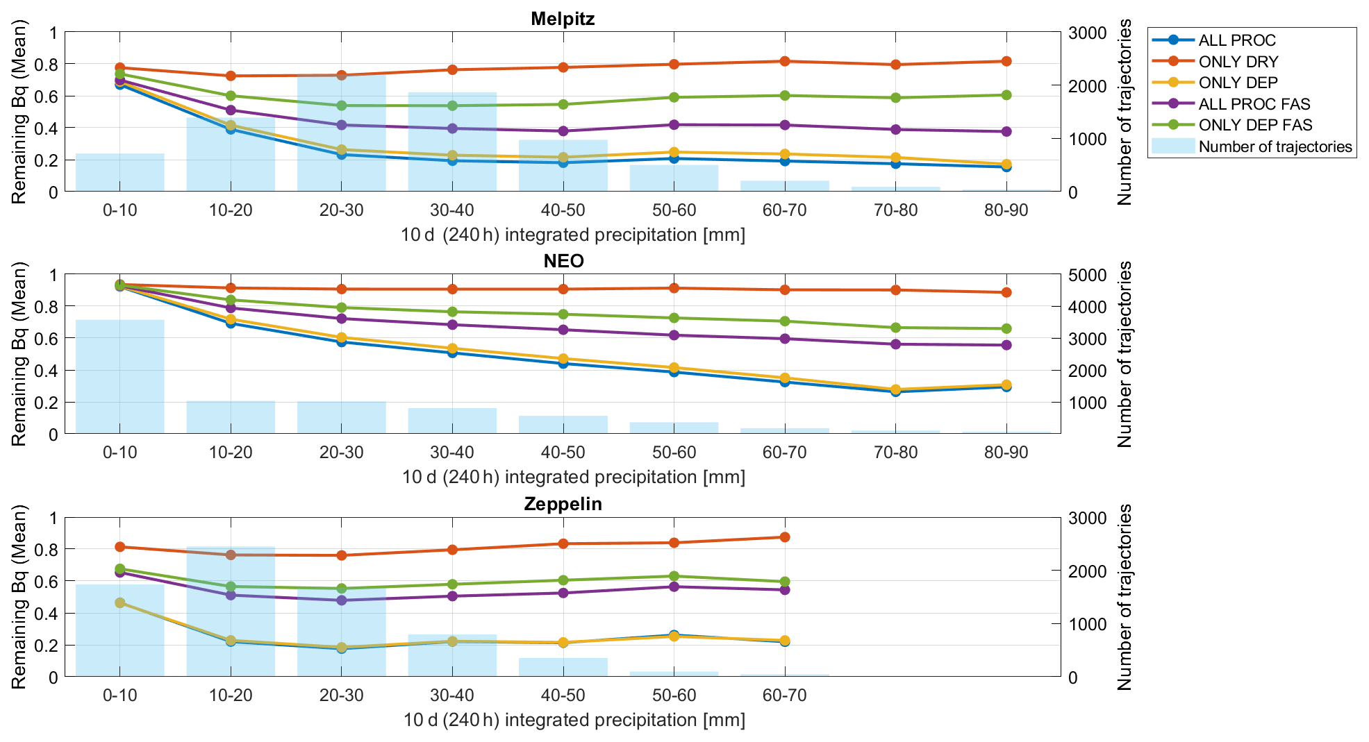
Figure 7 Total accumulated precipitation and caesium concentration at the end of the 10 d trajectories. The trajectories are binned with respect to its total accumulated precipitation (x axis). The mean final caesium concentration for all trajectories in each bin is plotted (left-hand y axis). The unit is normalized Becquerel values for each of the experiments. The number of trajectories in each bin is shown in blue bars (right-hand y axes).

The coupling between caesium concentration at the end of the 10 d simulations and the accumulated precipitation is illustrated in Fig. 7. The trajectories are binned with respect to the accumulated precipitation (i.e. all trajectories with 0–10 mm accumulated precipitation are in the first, trajectories with 10–20 mm accumulated precipitation are in the second and so forth). Mean values for all the trajectories in the respective bin are shown, with one line for each experiment. Blue bars are the number of trajectories in each bin (the right-hand y axes). Note that there were too few trajectories in bins with high amounts of precipitation for statistics, and bins with fewer than 30 trajectories have been filtered out. The maximum amount of accumulated 10 d precipitation is 100 mm for Melpitz, 150 mm for NEO and 99 mm for Zeppelin, and the lines end where there are no more cases. The ONLY DRY simulation (red line) is not affected by precipitation, and the variations due to the amount of precipitation is more coincidental but is visualized for reference.

For all stations, it is clear that the two experiments with advanced cloud simulations, ALL PROC (blue line) and ONLY DEP (yellow line), have the biggest reduction in caesium. They are also very similar to each other even though ONLY DEP has mostly slightly less remaining caesium. The two simulations with a fixed activation size, ALL PROC FAS and ONLY DEP FAS, have a substantially higher amount of caesium left compared to ALL PROC and ONLY DEP.

The experiments with advanced cloud parameterization (ALL PROC and ONLY DEP) have for Melpitz and Zeppelin an increasing caesium removal with more precipitation for the first bins (four bins for Melpitz at 0–40 mm and three bins for Zeppelin at 0–30 mm). Then the removal rate flattens out for higher precipitation amounts, and there is no clear change in the remaining caesium concentration. Note that there are very few trajectories in the bins with a high amount of precipitation, and changes here reflect more the behaviour of individual trajectories than a statistical average. The initial decrease of remaining caesium with higher precipitation amounts is also true for ALL PROC FAS and ONLY DEP FAS, but the decrease is not as strong as for ALL PROC and ONLY DEP. In NEO the final caesium concentration decreases between 0 and 80 mm of accumulated precipitation. For higher precipitation values, there is more irregular variations for NEO, which especially for the higher bins reflect individual trajectories more than a statistical average. This suggests that the fraction of aerosols available for wet removal decrease with time and that cloud formation mainly makes use of particles without ¹³⁷Cs formed during the simulations and thus does not affect the total ¹³⁷Cs concentration to a large extent. Thus, when the initial precipitation events have removed the bulk of Cs-containing particles, the remaining ¹³⁷Cs-containing particles are few, and cloud droplet activation takes place on newly formed particles without ¹³⁷Cs. The remaining caesium for Melpitz reaches 19 % of the released amount for ALL PROC, 23 % for ONLY DEP, 40 % for ALL PROC FAS and 54 % for ONLY DEP FAS. For Zeppelin the remaining caesium decreases until reaching 20–30 mm of precipitation. Higher levels of precipitation do not bring down the concentration much more (see comment about high precipitation levels above). Remaining caesium reaches 18 % for ALL PROC and ONLY DEP, 48 % for ALL PROC FAS and 55 % for ONLY DEP FAS. For NEO the decrease of the remaining Becquerel value does not flatten out as early; instead it continues to decrease with accumulated precipitation up to 70–80 mm. The air concentration after the 10 d period is then 27 % of the initial amount for both ALL PROC and ONLY DEP, 56 % for ALL PROC FAS and 66 % for ONLY DEP FAS.

Figure 7 shows the seasonal variation for the remaining caesium concentration after the 10 d simulations (monthly means in normalized Becquerel values). The largest reduction of caesium air concentration can be seen for all stations in the experiments ALL PROC and ONLY DEP, the experiments with advanced cloud parameterization. For these two experiments, there is a clear seasonal variation with higher remaining concentrations in the summer for Melpitz and NEO. Melpitz has the highest remaining concentration in May at 60 % and the lowest in January at 8 %. NEO has the highest values at 95 % in the 3 months of June–August and the lowest value of 47 % in February. The seasonal variability is not as strong for Zeppelin as it is for Melpitz and NEO.

The individual order between the different experiments are the same throughout the year for all three stations (except for the minor differences between ALL PROC and ONLY DEP in Zeppelin). ONLY DRY has the most remaining caesium (smallest reduction), followed by ONLY DEP FAS, ALL PROC FAS, and finally ONLY DEP and ALL PROC in the written order. The last two experiments are very similar in most cases.

Figure 8 Remaining caesium air concentration after the 10 d trajectories. Seasonal variation of monthly means for the different sites (Melpitz, a; NEO, b; and Zeppelin, c).

The previous figures have described the monthly and yearly mean averages. To better account for variability within the averaged time periods, we have analysed the behaviour of individual trajectories, thereby focusing on differences as percentile values for the different experiments. To analyse the impact of the full aerosol dynamic parameterization, these trajectory differences have been visualized in Fig. 9. The trajectory difference is defined as the difference of caesium air concentration at each time step in the 10 d simulation for two identical trajectories with different model physics (different experiments). It is shown as the difference in percentage points between the two experiments.

The trajectory difference between the experiments with the full model, ALL PROC, and the experiment with only dry deposition and cloud parameterization, ONLY DEP, is shown in the left column (ALL PROC minus ONLY DEP). This trajectory difference represents the impact that advanced aerosol dynamics have when added to a model using dry deposition and advanced cloud parameterization with wet deposition. The added processes include coagulation, condensational growth, nucleation and interaction with the background aerosol; involving new sources then creates the deviation from the 0 line in these plots. The trajectory difference between ALL PROC and ONLY DEP FAS is shown in the right column (ALL PROC minus ONLY DEP FAS). This shows the difference between a model with dry deposition and simplified cloud parameterization mimicking an LPDM simulation and a full-scale aerosol dynamic model (including advanced cloud parameterization and advanced aerosol dynamics). The percentiles in Fig. 9 show that there are outliers that does not follow the 0 line. Graphs on the 0 line indicate that there is no difference between the different experiments. The line for the Xth percentile shows the magnitude of the difference between the two experiments in X % of the trajectories (e.g. the 5th percentile represents the difference for 5 % of the simulations).

Figure 9 Difference in percentage points for the total caesium concentration for two different experiments. Percentile (Pctl) values over the 10 d period. ALL PROC minus ONLY DEP (a, c, e) and ALL PROC minus ONLY DEP FAS (b, d, f). Panels (a, b) are for Melpitz; (c, d) are for NEO; and (e, f) are for Zeppelin. Negative values represent when ALL PROC has lower concentration than the compared experiment (ONLY DEP on the left and ONLY DEP FAS on the right), i.e. when advanced aerosol dynamics yield lower air concentrations. Note that the scales of the y axes vary between the subplots.

After the 10 d period the 5th percentile is −11 % for Melpitz, −9 % for NEO and −7 % for Zeppelin for ALL PROC − ONLY DEP. The median (50th percentile) is slightly lower than the 0 line in Melpitz at −2 % after 10 d. In 75 % of the cases ALL PROC is smaller than ONLY DEP (the 75th percentile is slightly negative). It means that in 75 % of the cases including advanced aerosol dynamics makes the removal of caesium in the atmosphere more efficient. This is not true for NEO and Zeppelin, where the median (50th percentile) follows the 0 line. For all sites, there is a positive peak in the trajectory difference for the 75th, 90th and 95th percentiles in the beginning of the simulations, peaking just after the release. This originates from the release of the caesium gas and the condensation process that differs slightly between the experiments. This is most pronounced in the Zeppelin case, where the surface area of ambient particles available to condensate on is smaller due to fewer particles in Zeppelin. Since there are both negative and positive percentiles, including advanced aerosol dynamics can both increase and decrease the estimated air concentration of caesium. The magnitude of the trajectory difference is however larger when the ALL PROC simulations has lower concentrations than ONLY DEP.

The trajectory difference between a wet-deposition scheme mimicking an LPDM simulation, ONLY DEP FAS, and simulations with full aerosol dynamics, ALL PROC, can be seen in the right column of Fig. 9. The median for both Melpitz and Zeppelin is around −30 percentage points after the 10 d simulation (difference of 30 percentage points if using a simplified cloud interaction parameterization compared to full aerodynamic simulations). The median in NEO follows the 0 line. For 5 % of the simulations there is a difference of around −60 percentage points already after 5 d for all three stations. The 10th percentile after 5 d is −50 percentage points for Melpitz, −43 percentage points for NEO and −54 percentage points for Zeppelin. In this comparison of all cases (except for Zeppelin during the initial caesium condensation period) all percentile values are negative. The simulations mimicking an LPDM overpredict the air concentration of released caesium. This will in turn underpredict the deposition field.

4 Discussion

Considering the results in the previous section and keeping in mind the application for radiological emergency preparedness, we would like to highlight a few observations.

There are many different conditions and processes playing a role in the outcome of the simulated scenarios. The initial size distribution (Fig. 3) represents a key aspect in the setup of this study. The variability of the initial PNSD reflects both local and regional properties of the ambient aerosol and their relation to the sources, sinks and processes along the path it has taken to arrive at the site in question. During transport in the atmosphere, the interaction between condensation, coagulation and cloud processing (excluding precipitation) transforms an aerosol into the accumulation mode. Large particles in the coarse mode are rather rapidly removed due to gravitational settling, and particles on the smaller end of the size spectrum are rapidly grown into larger sizes through condensation or due to their small size removed either by dry deposition or by coagulation with larger-sized particles. Once in the accumulation mode, the only way of effectively removing the particles is through wet deposition in general and in-cloud scavenging in particular. As the lifetime for nucleation-mode particles and coarse-mode particles is short, long-range transport of ¹³⁷Cs is largely controlled by on the one hand how rapidly the released ¹³⁷Cs get partitioned into the accumulation mode, both directly via gas-to-particle conversion or indirectly by growth of smaller particles containing radioactive tracers. Once in the accumulation mode, the lifetime will largely be controlled by intensity and frequency of precipitation. The amount of time needed to partition the ¹³⁷Cs into the accumulation mode depends on how much of the aerosol is already there when the radioactive release starts. The characteristics of the initial aerosol PNSD also determine the effect that the different aerosol processes will have. Further, this will also connect to how the radionuclides initially are described. In our study we have assumed that the nuclides are emitted as a low-volatile vapour. Other assumptions could be emission of a pure combustion aerosol that dynamically will interact with the background aerosol. The nature of the emission scenario will of course therefore also affect the outcome of the study. The source fields that the trajectory box model travels through determine, together with the sinks, what new non-radioactive particles the radioactive aerosol will interact with in the simulated box. This occurs in this model setup when the box is within the mixing layer (depending on the trajectory path) which will make the PNSD differ from the ¹³⁷Cs activity size distribution. We have not studied the complexity near the source within the first day where aerosol dynamic processes might have a different impact, especially when it comes to releases in a highly polluted environment. To address the situation near the source other types of dispersion models are more suited than LPDMs, which is not within the scope of this study. The focus here has been on the result during and at the end of the 10 d simulation to understand the role of aerosol dynamics on this timescale. The meteorology clearly plays an important role for the outcome of each trajectory. It determines the path of the trajectory, horizontally as well as vertically. The meteorology also determines the conditions for clouds and therefore the air–cloud interactions and wet deposition, as well as the conditions for processes dependent on humidity, temperature and pressure. Since wet deposition is the most effective sink of the accumulation mode, the cases where there are clouds and precipitation have very different dynamics than the ones without clouds. The dynamical processes of condensational growth, coagulation, dry deposition, nucleation and chemical interactions take part in transforming the aerosol. They determine how the initial radioactive aerosol together with new sources are transformed into the accumulation mode. There is a difference in chemical composition for the particles in the different trajectories. This is important for droplet formation and wet deposition, which depend on the hygroscopicity of the particles. However, the focus in this study have been less on the dependence of chemical composition and more on the resulting PNSD and activity size distribution of caesium.

The change of the PNSD for the released radioactive caesium, attached on the surrounding particles, is visible in the annual averages in Fig. 4, and there are small but visible differences between the different sites. The decrease in total caesium concentration is much stronger in Melpitz and Zeppelin than in NEO. There are not-so-strong changes in the ¹³⁷Cs activity size distributions (relative change between small and large particles) in the annual averages. What can be seen is the just-mentioned decrease for Melpitz and Zeppelin and an ever-so-slight increase in the sizes of the caesium particles for NEO. Part of an explanation for this is that the initial surface area size distribution (Fig. 3) is often already located close to the accumulation mode around 0.1–1 µm, the size range that the aerosol processes strive to transform the aerosol towards. Wet deposition, the strongest sink for the aerosol in the accumulation mode is directly correlated with the precipitation. It explains the small change for the amount of caesium for NEO, since 46 % of the trajectories have very little precipitation, at 0–10 mm for the 10 d simulation (Fig. 6). Many of these cases are in the period June to mid-October (compare with total precipitation in Fig. 6), and it makes an impact on the annual average. It can also be seen in Fig. 8 that the reduction of caesium is small in the period June–September for NEO.

The impact of a good description of cloud interactions and wet deposition is visible in Fig. 7. The experiments with full cloud parameterization (ALL PROC and ONLY DEP) have a substantially more efficient removal of caesium than the experiments with a fixed activation size (ALL PROC FAS and ONLY DEP FAS). The findings suggest that the impact of aerosol dynamics is of lesser importance for the average dispersion and deposition patterns given that the wet deposition is handled sufficiently accurately. The results for ALL PROC and ONLY DEP are in this case very similar for all sites. If, for some reason, it is not possible to parameterize the cloud droplet activation well, then there is a benefit for including advanced aerosol dynamics (compare ONLY DEP FAS and ALL PROC FAS), since it decreases the air concentration further towards the experiment simulating all aerosol dynamic processes (ALL PROC) (Fig. 8). This is visible for all stations even though the effect is biggest for Melpitz (see the difference between ALL PROC FAS and ONLY DEP FAS).

The scavenging coefficient, a commonly used method both for in-cloud scavenging and below-cloud scavenging in an LPDM, is often derived from experiments. This inevitably creates a very close relationship between the model and the chosen experiments. This might not represent the variety of wet deposition that takes place in reality. The fixed activation size method, FAS, describes the creation of cloud droplets that might lead to wet scavenging of the aerosols which makes it more physically credible compared to a scavenging coefficient. The FAS method includes where in the column above and below the box cloud formation and precipitation occurs, whereas the scavenging coefficient only correlates ground level precipitation to the wet deposition with no height dependency. The coupling between activated particles and remaining particles for future activation is however neglected in the FAS parameterization. The activation size varies depending not only on the abundance of water vapour but also on the available particles. If there is still an environment for making new cloud droplets after a droplet-making event and all particles larger than the previous activation size are gone, then the activation size becomes smaller, leading to even smaller particles being activated. It makes this scheme sensitive for the choice of fixed activation size, and calculating this from current meteorological conditions and the current PNSD would be preferable. In the future, it would be interesting to have access to more cloud parameters from the numerical weather prediction models for better simulations of the air–cloud interaction and wet deposition.

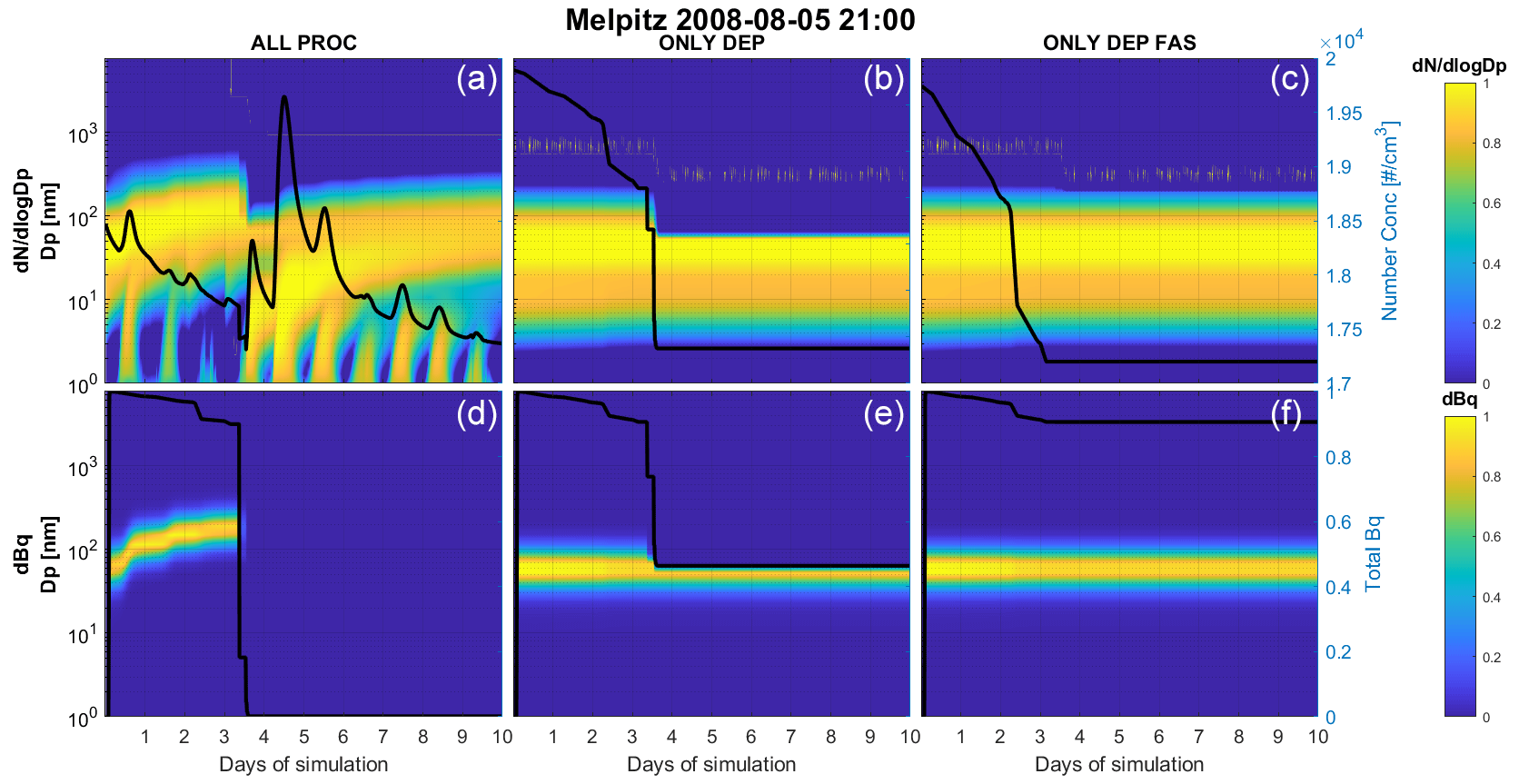
Figure 10 Result from one trajectory: Melpitz on 5 August 2008 at 21:00. Evolution of size distribution spectra for number concentration ($\text{d}N/\text{d}\log D_{\text{p}}$, normalized, a–c) and caesium concentration (dBq, normalized, d–f). Three different experiments: ALL PROC (a, d), ONLY DEP (b, e) and ONLY DEP FAS (c, f). The black lines represent total number concentration and total Becquerel concentration, respectively (axes to the right). Please note that the date in this figure is given in the format of year month day (yyyy-mm-dd).

The result of all the simulations when it comes to the mean values shows that including advanced aerosol dynamics does not always make a huge impact on the resulting caesium concentrations. It can be seen in Fig. 9 that the median (50th percentile) difference in the case with an advanced cloud parameterization scheme (left column) with and without aerosol dynamics is either close to zero for NEO and Zeppelin or 2 percentage points for Melpitz (at the end of the 10 d simulation). It implies that for statistical simulations, LPDMs can perform well without advanced aerosol dynamics as long as they model cloud physics closely. However, for decision support in emergency preparedness, the mean values are irrelevant; instead, the single realization at hand has to be simulated (for the current location and weather situation in question). In the 5th percentile there is a difference of 60 percentage points if aerosol processes together with an advanced cloud scheme are modelled (compared to using the simplified cloud interaction scheme, FAS, right column of Fig. 9). Also in the 25th percentile, there is a large difference of approx. 45 percentage points in the end of the simulation for Melpitz and Zeppelin and 20 percentage points for NEO. In a situation of radioactive hazard management, this difference could change a decision of whether to evacuate or not evacuate a certain area or how to deal with aspects of the food industry, such as crops and cattle. Taking severe actions brings also higher costs and complications for society and industry. The focus in this study is airborne concentration of the radioactive material, since that is the outcome of this model setup, while use of a dispersion model also calculates ground contamination (deposition fields). The conclusions made from airborne radioactivity concentration can be transferred to ground contamination, since they are directly linked. When the airborne concentration of radioactive material is reduced by wet deposition, it will create hotspots of deposited material on the ground. The location of these hotspots is very sensitive to each precipitation event, which may not be obvious when only analysing the air concentrations. Identifying these hotspots is still very important regarding mitigating actions. This could be a topic for a future study, since ground contamination is not a part of this study.

It can also be worth noting that including advanced aerosol dynamics, ALL PROC, compared to ONLY DEP (both using advanced air–cloud parameterization), can lead to both higher and lower air concentration (cf. Fig. 9, left). The percentiles are distributed on both sides of the 0 line. For Melpitz the 90th and 95th percentile is positive (higher concentration in ALL PROC than in ONLY DEP), and the rest are negative. For NEO the 50th percentile and higher are positive but quite close to zero, and the rest are negative with the 5th percentile on −9 percentage points after 10 d. The percentiles for Zeppelin on the other hand have a quite equal distribution on both sides of the 0 line with a maximum of 6 percentage points for the 95th percentile and −7 percentage points for the 5th percentile. It shows that advanced aerosol dynamics can either increase or reduce the air concentration depending on the site location and current weather parameters (while using advanced air–cloud parameterization).

As an illustration, we consider one realization (belonging to the 5th percentile) in Fig. 10. The top row shows the PNSD, and the bottom row shows the caesium distribution over time for the three different experiments, ALL PROC, ONLY DEP and ONLY DEP FAS, the same experiments used in the trajectory differences in Fig. 9. The black line represents the total number concentration and caesium concentration in respective plots. The trajectory enters a precipitation region after 3.5 d which can be seen in the ALL PROC simulation (left) as big particles are reduced (> 100 nm) and all the caesium located on those particles disappears quite instantly. In the ONLY DEP simulation (middle) the big particles also disappear, but all caesium does not. The caesium distribution in this case is the same as directly after the release, and the appearance remains throughout the simulation (no advanced aerosol dynamic processes are simulated). Therefore, a part of the caesium still remains in the air throughout the 10 d even though the bigger particles have deposited.

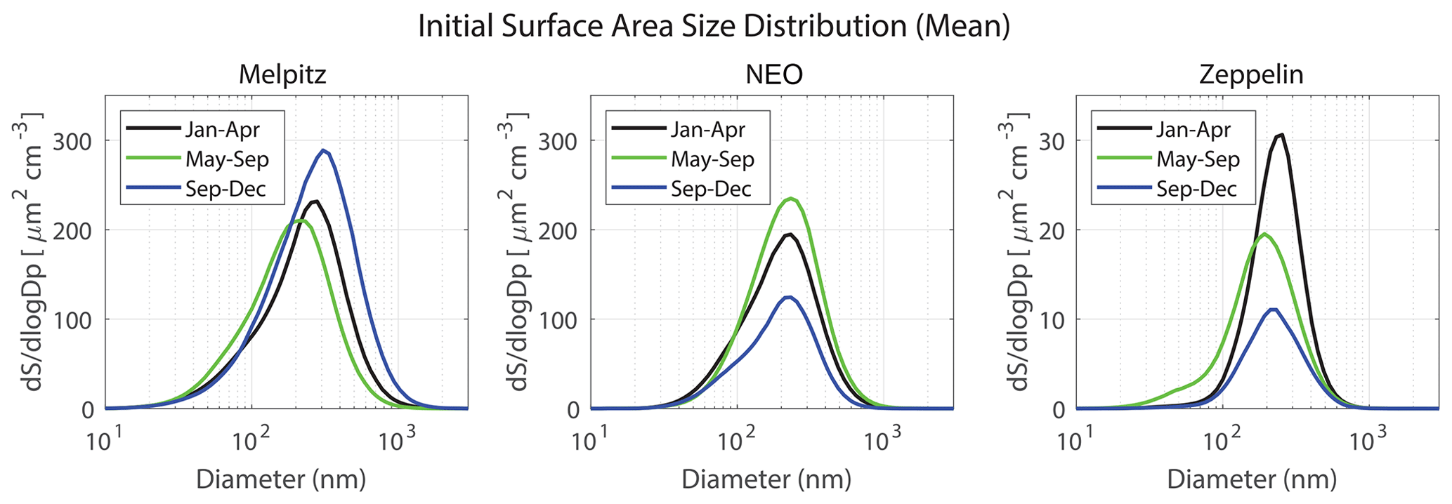
Figure 11 Surface area size distribution for measured ambient aerosol used to initiate each trajectory. Mean distributions for spring (January–April), summer (May–September) and autumn (September–December) for Melpitz, NEO and Zeppelin. The division into these time periods is taken from to emphasize differences between different periods. Note that the y axes have different scales for the different sites.

The activation size for ALL PROC and ONLY DEP is calculated from updraughts and humidity, and this size is clearly visible in the caesium concentration plot in Fig. 10 (middle column), since all particles above 60 nm are removed after about 3 d. In the ONLY DEP FAS simulation (right column of Fig. 10) almost all caesium is located on particles smaller than the fixed activation size, which makes the washout of caesium much less effective. After the precipitation event the remaining caesium is 0 % in the ALL PROC simulation, 46 % for ONLY DEP and 90 % of the initial amount for ONLY DEP FAS. These levels are reached directly after the precipitation period after about 3.5 d and stay throughout the rest of the simulations. This shows that advanced aerosol dynamics in ALL PROC transform the particles, with the aid of coagulation and condensational growth, bearing caesium into a size range where wet deposition via activation is predominant. Without this growth, the size of the Cs-bearing particles will not reach the size required for activation into cloud droplets. The result will be less efficient removal.

Comparing seasonal variations NEO stands out (Fig. 8). NEO has very low loss of Becquerel concentration in the air during the summer. This is due to the low amount of precipitation and clouds during the summer months for the NEO trajectories (see Fig. 6). Seasonal variations can also be seen in the Melpitz simulation especially in the experiment when all processes are turned on (cf. Fig. 8). This originates most likely from the initial caesium size distribution. The surface area size distribution of the measured ambient particles for the different stations can be seen in Fig. 11. Mean distributions are shown for the periods January–April, May–September and September–December. The periods are chosen from Fig. 8 to emphasize the differences of the characteristic seasons. The summer period for Melpitz, May–September, has the smallest surface area size distribution. This leads to less washout with the advanced air–cloud parameterization schemes, since the number of particles that are activated into cloud droplets are fewer and hence the seasonal variation in Fig. 8.

The effect of turning on and off processes is stronger (larger spread between the different experiments) for Melpitz and Zeppelin than for NEO in Fig. 8, especially in the beginning and the end of the year. For Zeppelin the seasonal variation is stronger after 5 d of simulations than after 10 d (see Fig. 4). In ALL PROC for Zeppelin the spread of monthly curves is much bigger around 5 d than at the end of the 10 d simulations, where they converge. It is clear in Fig. 11 that the seasonal variation in peak size of the particles is almost none in NEO but vary for both Melpitz and Zeppelin with the smallest diameters in summer. Melpitz has the most accumulated precipitation of all stations, and Zeppelin has the least. However, the effect of the simple cloud interaction scheme (fixed activation size) is strong for both Melpitz and Zeppelin even though the stations differ in total accumulated precipitation. The total number of particles in the air at Zeppelin varies over the year (Fig. 3), but compared to the other stations the total number concentration is generally low. When there are circumstances for droplet activation though, even smaller particles get activated, since the water vapour uses available particles for condensation. This leads to the biggest washout after the 10 d if all months are considered (Fig. 4), even though Zeppelin has the lowest amount of total precipitation of the three stations.

It can be argued that once a particle enters the accumulation-mode size range, its fate is largely controlled by the frequency and intensity of precipitation. Once this size has been reached, the particle will be comparably inert towards changes induced by condensation and coagulation and will retain its characteristics over long timescales. When the accumulation-mode size range is reached more simplified physical parameterization might be sufficient for the continuation of the simulation allowing for first-order treatment by either in-cloud or below-cloud scavenging. This would substantially limit computational costs compared to the concept of including all physiochemical aerosol dynamic modelling throughout the whole simulation.

5 Conclusions

To analyse the impact of including more advanced aerosol dynamics in LPDM simulations for radioactive releases, we have simulated single trajectories with a Lagrangian moving box model. For three different sites, a year of hourly measurements of the ambient PNSD initiated the model. To emulate the failure of a nuclear power plant, we released ¹³⁷Cs into the atmosphere, which then condensated on the ambient aerosol. The change of the PNSD and the radioactive activity size distribution were tracked all through a simulation time of 10 d. Five different experiments were made for each of the over 22 000 trajectories. The experiments represented different setups of the simulated processes. The simulated processes included coagulation, condensational growth, nucleation, additional sources of non-radioactive particles along the path, chemical interactions, and dry and wet deposition including aerosol–cloud interactions.

Comparing the mean values for the experiments simulating only dry and wet deposition including advanced cloud interactions and the full aerosol dynamic simulations shows small differences. For single events however the differences can be larger. For long-term statistical dispersion modelling having a good particle–cloud interaction scheme can therefore be sufficient. In a radioactive emergency situation, which is the topic of this study, single events can deviate from the statistical result, and more advanced parameterization might be necessary to adequately capture air concentration and deposition of radioactive material.

Precipitation brings the accumulation-mode particles to the ground, which emphasizes the importance of a good aerosol–cloud interaction parameterization scheme with wet deposition. We conclude that a good aerosol–cloud interaction scheme is the most important of the aerosol dynamic processes. If this is used together with dry deposition, the impact of including remaining aerosol processes can be described by the values of the concentration at the end of the 10 d simulations. We studied the magnitude of the difference between including or excluding the remaining aerosol processes for each trajectory in a statistical sense by considering percentiles. For 5 % of the simulations (5th percentile) there is a higher air concentration of 10 percentage points for all stations when only using the advanced aerosol–cloud interaction scheme as well as wet and dry deposition. In these cases, the processes of ambient dry aerosol increase the wet deposition. The 95th percentiles for Zeppelin and Melpitz are positive, which means that when all aerosol processes are included the radioactive particles are less prone to be activated for wet removal.

An aerosol–cloud interaction scheme with a fixed activation size is even more sensitive and generates a difference of 60 percentage points for the 5th percentile of the air concentration of ¹³⁷Cs after 10 d. That is, the air concentration is higher by 60 percentage points for the run with a fixed activation size compared to using the full aerosol dynamics. The deposition (not studied in detail in the current study) is directly linked to the air concentrations via wet and dry deposition, and development of possible hotspots is directly linked to the spatial and temporal timing of and the intensity of precipitation events. In this comparison there are no positive percentile values; i.e. including advanced aerosol dynamics always increases wet deposition. With a fixed activation diameter, in combination with omission of growth processes influencing the carried aerosol number size distribution, there is no way for the model to replenish the CCN. Thus, any process providing a mechanism growing the particles below the activation diameter to a size above it will enhance the overall deposition.

When simulating dispersion of radioactive material from a nuclear accident with an LPDM this study suggests that the following aspects should be considered:

• It is advisable to know and use best available information regarding the current ambient-aerosol PNSD onto which the emitted nuclides are condensated. Aspects of the chemical composition might also be important for hygroscopicity and reactivity with other species, but that has not been the focus of this study. How the initial size distribution surface properties will impact the deposition field and lifetime can be, to some degree, generalized as described in the following paragraphs:

  1. In general ambient conditions, the surface area is often already dominated by the accumulation mode. Cases where this applies require an adaptive activation scheme reflecting the competition between cloud droplet nucleation and/or growth and generation of supersaturation within the cloud. As this is true for a majority of the cases in this study, schemes with a fixed activation diameter will always underestimate the wet deposition if all other processes remain constant.

  2. If the initial carrier aerosol surface size distribution is to a large degree dominated by particles in the coarse mode (1 µm and above) the deposition field and lifetime of attached radionuclides attached will largely be controlled by dry deposition via sedimentation and impaction.

  3. In general ambient conditions, the surface area is often already dominated by the accumulation mode. Cases where this applies require an adaptive activation scheme reflecting the competition between cloud droplet nucleation and/or growth and generation of supersaturation within the cloud. As this is true for a majority of the cases in this study, schemes with a fixed activation diameter will always underestimate the wet deposition if all other processes remain constant.

• A good air–cloud interaction scheme in LPDMs is of greater importance than the other aerosol dynamic processes when air concentration is the result of the simulations that are of interest. If the sizes of the particles are important (for dose calculations, etc.), description of the evolution of the PNSD is important, and then all processes are needed.

• The seasonal variation of the remaining air concentration of released caesium (less in the summer) comes from variations in both initial surface area size distribution and in the amount of precipitation. The interaction between those two effects explains the similarities between the Melpitz and the Zeppelin result even though Melpitz has a higher particle number concentration and Zeppelin has much less precipitation.

• The range of simulated ¹³⁷Cs air concentrations for Melpitz and NEO grows with increasing time over the whole 10 d period, whereas for Zeppelin the spread grows the first 5 d and decreases after that (cf. Fig. 4). In Zeppelin eventually most of the particles are washed out at the end of the 10 d period. As long as there is precipitation that implies wet deposition, all ¹³⁷Cs particles will eventually be washed out. The time to wash out depends on the conditions for the individual trajectory and hence the meteorology, the season and the geographical location of the release event.

• It is also worth noting that while this study has focused on improving the description of the aerosol dynamical processes (model physics) to be included in an LPDM, the accuracy and the resolution of the numerical weather prediction model is of great importance for dispersion modelling. The numerical weather prediction model governs the simulation of the trajectories themselves (clouds, precipitation, meteorological parameters, and the path involving the distribution of the released material and the interaction with new sources along the way).

To conclude, the PNSD of the ambient aerosol and more advanced aerosol dynamic simulations are important in the case of simulating individual events, for example a release from a nuclear power plant. It would be interesting to expand this study with other geographical sites to broaden the knowledge of the impact of aerosol diversity.

The best way to include advanced aerosol dynamics in LPDMs to balance computational cost and the benefits of more detailed results needs to be dealt with in future studies, even though our results put an emphasis on advanced cloud interaction schemes. The data in this study can also be used for comparisons between different types of trajectories, e.g. over sea or over land, close to the surface, or high up in the atmosphere. This would be an interesting topic for future studies. In this paper we have shown the impact of including more advanced aerosol dynamic parameterizations in dispersion modelling for emergency preparedness. We hope that our results will spur a discussion between decision makers, scientists and modellers in devising the next generation of modelling tools for radiological preparedness.