the Creative Commons Attribution 4.0 License.
the Creative Commons Attribution 4.0 License.
 | 29 Mar 2021
The impact of cloudiness and cloud type on the atmospheric heating rate of black and brown carbon in the Po Valley
Asta Gregorič
Griša Močnik
Martin Rigler
Sergio Cogliati
Francesca Barnaba
Luca Di Liberto
Gian Paolo Gobbi
Niccolò Losi
Ezio Bolzacchini
We experimentally quantified the impact of cloud fraction and cloud type on the heating rate (HR) of black and brown carbon (HRBC and HRBrC). In particular, we examined in more detail the cloud effect on the HR detected in a previous study (Ferrero et al., 2018). High-time-resolution measurements of the aerosol absorption coefficient at multiple wavelengths were coupled with spectral measurements of the direct, diffuse and surface reflected irradiance and with lidar–ceilometer data during a field campaign in Milan, Po Valley (Italy). The experimental set-up allowed for a direct determination of the total HR (and its speciation: HRBC and HRBrC) in all-sky conditions (from clear-sky conditions to cloudy). The highest total HR values were found in the middle of winter (1.43 ± 0.05 K d−1), and the lowest were in spring (0.54 ± 0.02 K d−1). Overall, the HRBrC accounted for 13.7 ± 0.2 % of the total HR, with the BrC being characterized by an absorption Ångström exponent (AAE) of 3.49 ± 0.01. To investigate the role of clouds, sky conditions were classified in terms of cloudiness (fraction of the sky covered by clouds: oktas) and cloud type (stratus, St; cumulus, Cu; stratocumulus, Sc; altostratus, As; altocumulus, Ac; cirrus, Ci; and cirrocumulus–cirrostratus, Cc–Cs). During the campaign, clear-sky conditions were present 23 % of the time, with the remaining time (77 %) being characterized by cloudy conditions. The average cloudiness was 3.58 ± 0.04 oktas (highest in February at 4.56 ± 0.07 oktas and lowest in November at 2.91 ± 0.06 oktas). St clouds were mostly responsible for overcast conditions (7–8 oktas, frequency of 87 % and 96 %); Sc clouds dominated the intermediate cloudiness conditions (5–6 oktas, frequency of 47 % and 66 %); and the transition from Cc–Cs to Sc determined moderate cloudiness (3–4 oktas); finally, low cloudiness (1–2 oktas) was mostly dominated by Ci and Cu (frequency of 59 % and 40 %, respectively).
HR measurements showed a constant decrease with increasing cloudiness of the atmosphere, enabling us to quantify for the first time the bias (in %) of the aerosol HR introduced by the simplified assumption of clear-sky conditions in radiative-transfer model calculations. Our results showed that the HR of light-absorbing aerosol was ∼ 20 %–30 % lower in low cloudiness (1–2 oktas) and up to 80 % lower in completely overcast conditions (i.e. 7–8 oktas) compared to clear-sky ones. This means that, in the simplified assumption of clear-sky conditions, the HR of light-absorbing aerosol can be largely overestimated (by 50 % in low cloudiness, 1–2 oktas, and up to 500 % in completely overcast conditions, 7–8 oktas).
The impact of different cloud types on the HR was also investigated. Cirrus clouds were found to have a modest impact, decreasing the HRBC and HRBrC by −5 % at most. Cumulus clouds decreased the HRBC and HRBrC by −31 ± 12 % and −26 ± 7 %, respectively; cirrocumulus–cirrostratus clouds decreased the HRBC and HRBrC by −60 ± 8 % and −54 ± 4 %, which was comparable to the impact of altocumulus (−60 ± 6 % and −46 ± 4 %). A higher impact on the HRBC and HRBrC suppression was found for stratocumulus (−63 ± 6 % and −58 ± 4 %, respectively) and altostratus (−78 ± 5 % and −73 ± 4 %, respectively). The highest impact was associated with stratus, suppressing the HRBC and HRBrC by −85 ± 5 % and −83 ± 3 %, respectively. The presence of clouds caused a decrease of both the HRBC and HRBrC (normalized to the absorption coefficient of the respective species) of −11.8 ± 1.2 % and −12.6 ± 1.4 % per okta. This study highlights the need to take into account the role of both cloudiness and different cloud types when estimating the HR caused by both BC and BrC and in turn decrease the uncertainties associated with the quantification of their impact on the climate.
- Article
(8815 KB) - Full-text XML
-
Supplement
(29291 KB) - BibTeX
- EndNote


The impact of aerosols on the climate is traditionally investigated with a focus on their direct, indirect and semi-direct effects (Bond et al., 2013; IPCC, 2013; Ferrero et al., 2018, 2014; Ramanathan and Feng, 2009; Koren et al., 2008, 2004; Kaufman et al., 2002). Direct effects are related to the sunlight interaction with aerosols through absorption and scattering; indirect effects are related to the ability of aerosol to act as cloud condensation nuclei affecting the cloud formation and properties; and semi-direct effects are those related to a feedback on cloud evolution affecting other atmospheric parameters (e.g. the thermal structure of the atmosphere) (IPCC, 2013; Ramanathan and Feng, 2009; Koren et al., 2008, 2004; Kaufman et al., 2002). Both direct and indirect radiative effects of anthropogenic and natural aerosols are still the major sources of uncertainties on climate (IPCC, 2013). Recent studies show, for example, that the aerosol direct radiative effect (on a global scale) may switch from positive to negative forcing on short (e.g. daily) timescales (Lolli et al., 2018; Tosca et al., 2017; Campbell et al., 2016). This is due to the fact that aerosol is a heterogeneous complex mixture of particles characterized by different size, chemistry and shape (e.g. Costabile et al., 2013), greatly varying in time and space both in the horizontal and vertical dimension (e.g. Ferrero et al., 2012). On a global scale, most of the values reported for the aerosol direct radiative effect were derived from models (Bond et al., 2013; Koch and Del Genio, 2010). This has the advantage of providing fields of continuous direct radiative effect in space and time. However, inaccuracies related to simplified model assumptions on chemistry, shape and the mixing state of particles can affect the results (Nordmann et al., 2014; Koch et al., 2009); this amplifies the uncertainties on the related global and regional aerosol effects on the climate (Andreae and Ramanathan, 2013). The aerosol direct radiative effect has been usually determined in clear-sky conditions both in model simulations and measurements. The clear-sky approximation is useful when comparing measurements to radiative-transfer modelling outcomes during experimental campaigns performed in fair-weather conditions (e.g. Ferrero et al., 2014; Ramana et al., 2007); however, in general this simplification cannot capture the complexity of the phenomenon in the majority of weather conditions (Myhre et al., 2013). In fact, clouds are one of the most important factors influencing the solar radiation reaching the ground. By scattering and absorbing the radiation, clouds can affect the radiation magnitude and modify its spectrum, especially in the ultraviolet (UV) region (López et al., 2009; Thiel et al., 2008; Calbó et al., 2005). During cloudy conditions the global irradiance is usually reduced; however, the presence of clouds sometimes results in short-term enhancement of global irradiance (Duchon and O'Malley, 1999). In some specific cases, the scattering of radiation from the sides of the cloud may enhance global irradiance in the UV to the levels higher than those in clear-sky conditions (Mims and Frederick, 1994; Feister et al., 2015). Mims and Frederick (1994) determined that the scattering from the sides of cumulus clouds can enhance the total (global) UV-B solar irradiance by 20 % or more over the maximum solar-noon value when cumulus clouds were close to (but not when blocking) the solar disk. In a similar way, Feister et al. (2015) concluded that the scattering of solar radiation by clouds can enhance UV irradiance at the surface – for example, cumulonimbus clouds, with top heights close to the tropical tropopause layer, have the potential to significantly enhance diffuse UV-B radiance over its clear-sky value. UV radiation also interacts with aerosols and particularly with those featuring significant absorption values in this spectral region. UV represents an important region for brown carbon (BrC) absorption with respect to other light-absorbing aerosol (LAA) components (e.g. black carbon, BC). Thus, the presence of clouds could influence the impact of different LAA species on the climate in a different way.
Up to now, the role of cloudiness and cloud type on the aerosol direct radiative effect was poorly investigated. Matus et al. (2015) recently used a complex combination of the CloudSat's satellite multi-sensor radiative flux and heating-rate (HR) products to infer both the direct radiative effect at the top of the atmosphere and HR profiles of aerosols that lie above the clouds. The study showed how results were affected by the cloudiness (e.g. cloud fraction) and, for the southeastern Atlantic, reported a direct radiative effect ranging from −3.1 to −0.6 W m−2, going from clear-sky to cloudy conditions.
A further investigation by Myhre et al. (2013) reported results of modelling simulations during the AeroCom (Phase II) project: in all-sky conditions (thus including the effect of clouds) they estimated an all-sky direct radiative effect of −0.27 W m−2 (range of −0.58 to −0.02 W m−2) for total anthropogenic aerosols, with this being about half of the clear-sky one. The most important factors responsible for the observed difference were the amount of aerosol absorption and the location of aerosol layers in relation to clouds (above or below). In fact, the presence of LAA (mainly BC, BrC and mineral dust) might have important effects on the radiative balance. It is estimated that, due to its absorption of sunlight, BC is the second most important positive anthropogenic climate forcer after CO2 (Bond et al., 2013; Ramanathan and Carmichael, 2008); BrC contributes ∼ 10 %–30 % to the total absorption on a global scale (Ferrero et al., 2018; Kumar et al., 2018; Shamjad et al., 2015; Chung et al., 2012). As a main difference compared to CO2, LAA species are short-lived climate forcers, thus representing a potential global warming mitigation target. However, the real potential benefit of any mitigation strategy should also be based on observational measurements, possibly carried out in all-sky conditions.
It also noteworthy that the HR induced by LAA can trigger different atmospheric feedbacks. BC and mineral dust can alter the atmospheric thermal structure, thus affecting the atmospheric stability, the cloud distribution and even the synoptic winds such as the monsoons (IPCC, 2013; Bond et al., 2013; Ramanathan and Feng, 2009; Koch et al., 2009; Ramanathan and Carmichael, 2008; Koren et al., 2008, 2004; Kaufman et al., 2002). These feedbacks should be quantified on the basis of HR measurements in all-sky conditions. In agreement with this, both Andreae and Ramanathan (2013) and Chung et al. (2012) called for model-independent, observation-based determination of the absorptive direct radiative effect of aerosols. Since cloudiness and cloud type change on short timescales similarly to aerosols, long-term, highly time-resolved measurements (covering different sky conditions) are necessary to unravel the impact of LAA on the HR.
Satellite-based studies investigated the role of cloudiness and cloud type on the HR of aerosol layers above clouds (Matus et al., 2015). To our knowledge, there has been no experimental investigation of cloudiness and cloud type impact on the HR of aerosol layers below clouds, where most of the aerosol pollution typically resides. Cloud–aerosol feedbacks can strongly depend on the HR magnitude in cloudy conditions. As a matter of fact, the atmospheric heating induced by absorbing aerosol is traditionally related to a decrease of atmospheric relative humidity and less cloud cover (semi-direct effect). This effect can further increase the amount of the incoming solar radiation that reaches Earth's surface (and any close-to-surface LAA layers), leading to a positive feedback characterized by additional warming and a further decrease in the cloud amount (e.g. Koren et al., 2004). However, Perlwitz and Miller (2010) reported a counterintuitive feedback: the atmospheric heating induced by tropospheric absorbing aerosol could lead to a cloud cover increase (especially low-level clouds) due to a delicate interplay between relative humidity and temperature. The study concluded that high absorption by aerosols was responsible for two counteracting processes: a large diabatic heating of the atmospheric column (thus decreasing relative humidity) and a corresponding increase in the specific humidity able to exceed the temperature effect on relative humidity, with the net result of increasing low cloud cover with increasing aerosol absorption. This is an important result that underlines the importance of measuring the atmospheric HR in cloudy conditions as a constraint and/or input for more comprehensive climate models to shed light on the sign and magnitude of the related feedbacks on cloud dynamics.
This study attempts to experimentally measure for the first time the impact of different cloudiness levels and cloud types on the HR exerted by near-surface LAA species. The study was performed in Milan (Italy), located in the middle of the Po Valley (Sect. 2), which is an air pollution hotspot in Europe; its meteorological conditions are similar to those of a multitude of basin valleys (surrounded by hills or mountains) in which low wind speeds and stable atmospheric conditions promote the accumulation of aerosol (Zotter et al., 2017; Moroni et al., 2013, 2012; Ferrero et al., 2013, 2011a; Barnaba et al., 2010; Carbone et al., 2010; Rodriguez et al., 2007). Cloud presence cannot be neglected over the investigated area considering that, in the last 50 years, the annual average cloudiness, expressed in oktas, was estimated to be ∼ 5.5 over Europe (Stjern et al., 2009) and ∼ 4 over Italy (Maugeri et al., 2001). This feature is similar to 80 years of data of cloud cover in the United States (Crocke et al., 1999). To determine the LAA HR, we used a methodology previously developed in Ferrero et al. (2018) and further extended here to explore the effects of cloudiness and different cloud types on the HR of BC and BrC. More specifically, this work introduces the following novelties: (1) it describes the interaction between cloudiness and light-absorbing aerosol, presenting the aerosol HR as a function of cloudiness, and in turn estimates the systematic bias introduced by incorrectly assuming clear-sky conditions in radiative-transfer models; (2) it introduces a cloud type classification and investigates the impact of both cloudiness and cloud types on the total HR; and (3) it separates BC and BrC contributions and investigates their relative impact on the total HR as a function of sky conditions. The results presented in this study add an important piece of information in the general context of cloud–aerosol interactions and their influence on the HR.
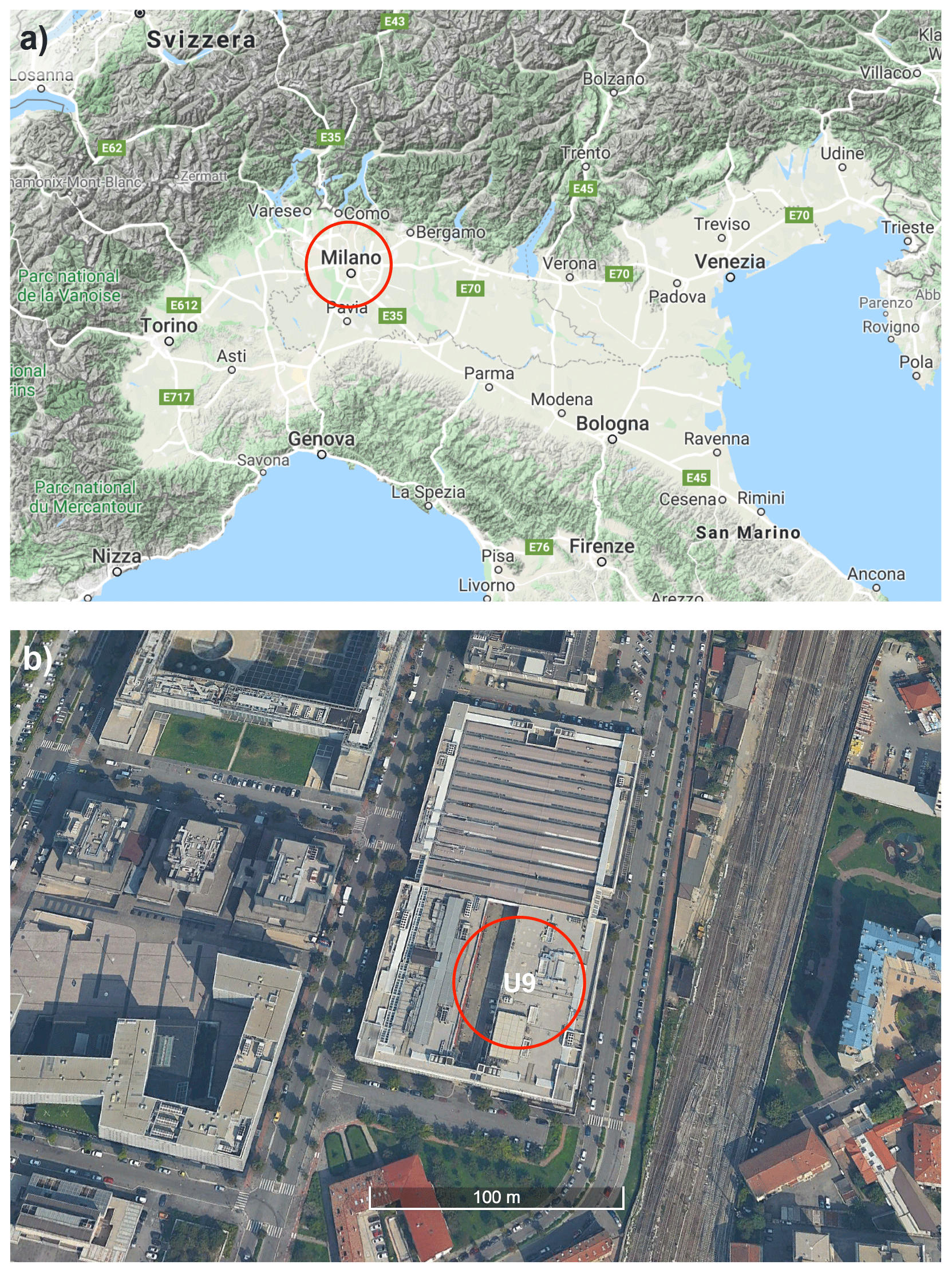
Figure 1(a) Location of the Milan sampling site in the Po Valley, Italy; (b) the U9 sampling site on the rooftop (10 ) of the University of Milano-Bicocca. The copyright holder of Fig. 1 is Google Maps (© Google Maps).
Aerosol, cloud and spectral irradiance were measured in Milan (Italy) on the rooftop (10 ) of the U9 building of the University of Milano-Bicocca (45∘ 30′38′′ N, 9∘12′42′′ E; Italy; Fig. 1). The site is located in the midst of the Po Valley, one of the most industrialized and heavily populated areas in Europe. In the Po Valley, stable atmospheric conditions often occur, causing a marked seasonal variation of aerosol concentrations within the mixing layer (Barnaba et al., 2010), well visible even from satellites (Ferrero et al., 2019; Di Nicolantonio et al., 2007, 2009; Barnaba and Gobbi 2004). A full description of the aerosol behaviour in Milan, at the University of Milano-Bicocca, and of the related properties (vertical profiles, chemistry, hygroscopicity, sources and toxicity) is reported in previous studies (Diemoz et al., 2019a; Lorelei et al., 2019; D'Angelo et al., 2016; Curci et al., 2015; Ferrero et al., 2015, 2010; Sangiorgi et al., 2011, 2014; Sandrini et al., 2014). In the framework of the present work it is important to underline that the U9 experimental site is particularly well suited for atmospheric radiation measurements: it is characterized by a full hemispherical sky view and equipped with the instruments described in Sect. 2.1. The measurement set-up allowed for the experimental determination of the instantaneous aerosol HR (K d−1) induced by absorbing aerosol as detailed in Sect. 2.2. The methodological approach used to quantify the cloud fraction and to classify the cloud type is reported in Sect. 2.3. Finally, Appendix A resumes the nomenclature used in the present work.
2.1 Instruments
The aerosol, cloud and radiation instrumentations have been installed at the U9 sampling site in Milan since 2015. The site location is shown in Fig. 1. The complete instrumental set-up (Fig. S1 in the Supplement) is described hereafter.
2.1.1 Light-absorbing aerosol measurements and apportionment
Measurements of the wavelength-dependent aerosol absorption coefficient babs(λ) were obtained using a Magee Scientific AE-31 aethalometer. This allowed for multi-spectral measurements (7-λ: 370, 470, 520, 590, 660, 880 and 950 nm) in the wide UV–VIS–NIR (ultraviolet–visible–near-infrared) region, not available from other instruments (e.g. multi-angle absorption photometer, MAAP; particle soot absorption photometer, PSAP; and photoacoustic) (Virkkula et al., 2010; Petzold et al., 2005). This spectral range is needed for the HR determination (Sect. 2.2). The use of aethalometers also presents the advantage of global long-term data series (Ferrero et al., 2016; Eleftheriadis et al., 2009; Collaud Coen et al., 2010; Junker et al., 2006) that could allow for deriving historical data of the HR in the future.
To account for both the multiple-scattering enhancement (the elongation of the optical path induced by the filter fibres) and the loading effects (the non-linear optical path reduction induced by absorbing particles accumulating in the filter), the AE-31 data were corrected by applying the Weingartner et al. (2003) procedure (Ferrero et al., 2018, 2014, 2011b; Collaud Coen et al. 2010). As detailed by Collaud Coen et al. (2010), the Weingartner et al. (2003) procedure compensates for all the aethalometer artefacts (the backscattering is indirectly included within the multiple-scattering correction), showing a good robustness (negative values are not generated, and the results are in good agreement with other filter photometers), and, most importantly, it does not affect the derived aerosol absorption Ångström exponent (AAE) (fundamental for HR determination, Sect. 2.2). Overall, the multiple-scattering parameter C was 3.24 ± 0.03, as obtained by comparing the AE-31 data at 660 nm with an MAAP at a very similar wavelength (637 nm, Müller et al., 2011) (regression between AE-31 and MAAP in Fig. S2 in the Supplement). This value lies very close to that suggested by the Global Atmosphere Watch (GAW) programme (WMO/GAW, 2016), i.e. C = 3.5. The physical meaning of the similarity between the obtained C value (3.24 ± 0.03) and the GAW one implies that Milan (in the middle of the Po Valley) is characterized by continental-type aerosols (e.g. Carbone et al., 2010) and consistent with the global average. To verify the reliability of the obtained C value, it was also computed following the Collaud Coen et al. (2010) procedure. They defined the reference value of C (Cref = 2.81 ± 0.11) for the AE-31 tape based on data from pristine environments (Jungfraujoch and Hohenpeissenberg sites, where aerosol has a single-scattering albedo of ∼ 1); at the same time, Collaud Coen et al. (2010) defined C for any type of aerosol as follows:
where α is the parameter for the Arnott et al. (2005) scattering correction (0.0713 at 660 nm) and ω0 the single-scattering albedo. In wintertime in Milan, within the mixing layer, the single-scattering albedo was found to be 0.846 ± 0.011 at 675 nm by Ferrero et al. (2014). From Eq. (1), it follows that the computed C in Milan is 3.20 ± 0.35, in keeping with the experimental one (3.24 ± 0.03). Details concerning wavelength differences are discussed in the Supplement (“Measured and computed C factor”). The loading effects were dynamically determined following the Sandradewi et al. (2008b) approach, while the final equivalent BC (eBC) concentrations were obtained applying the AE-31 apparent mass attenuation cross section (16.6 m2 g−1 at 880 nm).
The abovementioned compensation procedures introduce an uncertainty in the absorption coefficient measurements. Collaud Coen et al. (2010) tested these procedures in different locations and estimated the global accuracy of the Weingartner et al. (2003) correction (applied in the present work) to be ∼ 23 %. Moreover, Drinovec et al. (2015) showed a good agreement between AE-31 aethalometer data (corrected using Weingartner et al., 2003) and those of the new version, AE-33, with a slope close to unity and R2 > 0.90. Thus, the Collaud Coen et al. (2010) accuracy estimation is considered as the worst scenario.
As the spectral signature of the aerosol absorption coefficient babs(λ) reflects the different nature of absorbing aerosol (BC and BrC), once babs(λ) is obtained, it can be apportioned to determine the contributions of BC and BrC, respectively. This result can be achieved considering that BC aerosol absorption is characterized by an absorption Ångström exponent, AAE ≈ 1 (Massabò et al., 2015; Sandradewi et al., 2008a; Bond and Bengstrom, 2006). Conversely, BrC absorption is spectrally more variable, with an AAE from 3 to 10 (Ferrero et al., 2018; Shamjad et al., 2015; Massabò et al., 2015; Srinivas and Sarin, 2013; Yang et al., 2009; Kirchstetter et al., 2004). The wavelength dependence of the absorption coefficient of BrC can be described by the simple harmonic oscillator reported in Moosmüller et al. (2011): the much lower absorption in the IR (infrared) region (compared to UV) is a consequence of the resonances in the UV from which the IR region is far removed. This calculation also yields to decreasing AAE values with increasing wavelengths. This is equivalent to the band-gap model with the Urbach tail as detailed in Sun et al. (2007) and references in Moosmüller et al. (2011), where the key factor is the difference between the highest occupied and lowest unoccupied energy state of the molecules included in the BrC ensemble. In this study we determined AAEBrC following the innovative apportionment method proposed by Massabò et al. (2015). This allows for apportioning babs(λ) to BC and BrC and for determining, at the same time, the AAEBrC assuming that all BrC results from biomass burning. The method by Massabò et al. (2015) was previously applied to the Milan U9 measurements leading to an annual average of AAEBrC = 3.66 ± 0.03 (Ferrero et al., 2018).
2.1.2 Radiative, meteorological and lidar measurements
Spectral irradiance measurements were collected using a multiplexer–radiometer–irradiometer (MRI; Fig. S1; details in Cogliati et al., 2015) which resolves the UV–VIS–NIR spectrum (350–1000 nm) in 3648 spectral bands (3648-element linear CCD array detector; charge-coupled device; Toshiba TCD1304AP, Japan) for both the downwelling and the upwelling radiation fluxes. The instrument was developed at the University of Milano-Bicocca using an optical switch (MPM-2000-2x8-VIS, Ocean Optics Inc., USA) to sequentially select between different input fibres fixed to up- and down-facing entrance fore-optics. The configuration used in the present work connects each spectrometer to three input ports: (1) the CC-3 cosine-corrected irradiance probes to collect the downwelling irradiance, (2) the bare fibre optics with a 25∘ field of view to measure the upwelling radiance from the terrestrial surface and (3) the blind port that is used to record the instrument dark current. A 5 m long optical fibre with a bundle core with a diameter of 1 mm is used to connect the entrance fore-optics to the multiplexer input, while the connection between the multiplexer output ports and the spectrometers is obtained with 0.3 m long optical fibres. The set-up allows for sequentially measuring dark current and both up- and downwelling spectra simultaneously with the two spectrometers. The two spectrometers used are high-resolution HR4000 holographic grating spectrometers (Ocean Optics Inc., USA). Finally, the multiplexer–radiometer–irradiometer was equipped with a rotating shadow band to measure separately the spectra of the direct, diffuse and reflected irradiance (Fdir(λ), Fdif(λ), Fref(λ)). The reflected irradiance originated from a Lambertian concrete surface (due to its flat and homogeneous characteristics which represents the average spectral reflectance of the Milan urban area well; Ferrero et al, 2018).
Broadband (300–3000 nm) downwelling (global and diffuse) and upwelling (reflected) irradiance measurements were also collected using LSI Lastem radiometers (DPA154 and C201R, class 1, ISO 9060, 3 % accuracy). Diffuse broadband irradiance was measured using the DPA154 global radiometer equipped with a shadow band whose effect was corrected (Ferrero et al., 2018) to determine the true amount of both diffuse and direct (obtained after subtraction from the global) irradiance. Next, MRI spectra were normalized and completed with normalized literature spectra (Ferrero et al., 2018) to cover the broadband range (300–3000 nm) and irradiance intensity measured by standard LSI Lastem pyranometers, allowing for the HR to be evaluated over the whole short-wave range (babs(λ) was estimated outside the AE-31 range using its AAE). The approach was previously validated (Ferrero et al., 2018): the HR in the strict UV–VIS–NIR range (350–950 nm of the AE31 and the MRI) accounted on average for 86.4 ± 0.4 % of the total broadband values.
In addition to radiation measurements, temperature, relative humidity, pressure and wind parameters were measured using the following LSI Lastem sensors: DMA580 and DMA570 for thermo-hygrometric measurements (for T and RH: range of −30– +70 ∘C and 10 %–98 %, accuracy of ± 0.1 ∘C, and ± 2.5 % sensibility of 0.025 ∘C and 0.2 %), the CX110P barometer model for pressure (range of 800–1100 hPa and accuracy of 1 hPa) and the CombiSD anemometer (range of 0–60 m s−1 and 0–360∘) for wind measurements.
The experimental station U9 is also equipped with an automatic lidar–ceilometer operated by ISAC-CNR in the framework of the Italian Automated LIdar-CEilometer network (ALICEnet, http://www.alice-net.eu, last access: 22 March 2021) and contributes to the EUMETNET (European meteorology network) E-Profile network (https://www.eumetnet.eu/, last access: 22 March 2021). This is a Jenoptik Nimbus 15k biaxial lidar–ceilometer operating 24 h d−1, 7 d per week. It is equipped with an Nd:YAG (neodymium-doped yttrium aluminium garnet) laser that emits light pulses at 1064 nm with an energy of 8 µJ per pulse and a repetition rate of 5 kHz. The backscattered light is detected by an avalanche photodiode in the photon-counting mode (Wiegner and Geiß, 2012; Madonna et al., 2015). The vertical and temporal resolution of the raw signals are 15 m and 30 s, respectively. In order to improve the signal-to-noise ratio of the backscatter signal, the signal is processed with temporal averages of 2 min. The full overlap is obtained at an altitude of some hundred metres above the observation site, and overlap correction functions are applied in the first layers. The Nimbus 15k lidar–ceilometer is able to determine cloud base height (CBH), penetration depth, and with specific processing mixing layer height and vertical profiles of aerosol optical and physical properties (e.g. Diemoz et al., 2019a, b; Dionisi et al., 2018). We used the U9 ceilometer data for cloud layering and relevant cloud base height, as the system can reliably detect multiple cloud layers and cirrus clouds (Wiegner et al., 2014; Boers et al., 2010; Martucci et al., 2010) within its operating vertical range (up to 15 km). Given the vertical resolution of the instrument, expected uncertainty of the cloud base height derived by the lidar–ceilometer is less than ± 30 m.
Global and diffuse irradiance measurements, coupled with the ceilometer data, were used to determine the sky cloud fraction and to classify the cloud types by following the methodology presented in the Sect. 2.3.
2.2 Heating-rate measurements
The instantaneous aerosol HR (K d−1) induced by LAA is experimentally obtained using the methodology reported and validated in Ferrero et al. (2018), where the reader is referred to for the details of the approach. Here we briefly summarize the method.
The heating rate is determined from the air density (ρ, kg m−3); the isobaric specific heat of dry air (Cp, 1005 ); and the radiative power absorbed by aerosol per unit volume of air (W m−3), which describes the interaction between the radiation (either direct from the sun, diffused by atmosphere and clouds, and reflected from the ground) and the LAA (BC and BrC in Milan). The HR is determined as follows (Ferrero et al., 2018):
where the subscripts dir, dif and ref refer to the direct, diffuse and reflected components of the spectral irradiance F of wavelength λ impinging on LAA with a zenith angle θ (from any azimuth).
Under the isotropic and Lambertian assumptions (as used in Ferrero et al., 2018), Eq. (2) can be solved, becoming
where θz refers to the solar zenith angle, while Fdir(λ), Fdif(λ) and Fref(λ) are the spectral direct, diffuse and reflected irradiances. Equations (2) and (3) are related to the concept of actinic flux (Tian et al., 2020; Gao et al., 2008; Liou, 2007); an extended description, as well as its demonstration, is detailed in the Supplement.
As the intensity of the irradiance components is a function of cloudiness and cloud type (Sect. 2.3), Eq. (3) enables assessing the impact of the latter components on the aerosol absorption of short-wave radiation and thus on the corresponding HR (Sects. 3.2 and 3.3).
The most important advantages and limitations of this measurement-based approach to derive the LAA HR are as follows. The advantages are as follows:
-
no radiative-transfer assumptions needed (i.e. no assumption of clear-sky conditions), as the parameters input to Eq. (3) are all measured quantities;
-
possibility to follow the rapid HR dynamic to investigate the HR temporal evolution, as measurements of spectral irradiance and absorption coefficient are carried out with high temporal resolution; and
-
possibility to derive the HR in all-sky conditions, as measurements of spectral irradiance and the absorption coefficient are independent from atmospheric conditions enabling us to investigate the impact induced by the clouds.
The limitation is as follows:
-
The HR is independent of the thickness of the investigated atmospheric layer and refers to the vertical location of the atmospheric layer in which it is experimentally determined. In the present work the HR was determined into the near-surface atmospheric layer.
With respect to this limitation, it should be mentioned that BC and HR vertical profile data previously collected at the same site and in other valley basins revealed that the HR was constant inside the mixing layer (Ferrero et al., 2014). In fact, above our observational site, vertical profile measurements with a tethered balloon and a lidar–ceilometer have been performed since 2005, mostly showing homogeneous concentrations of aerosol (and related extinction coefficient) within the mixing layer, particularly in daytime (Ferrero et al., 2019). The same condition was verified by the lidar–ceilometer data collected during the present campaign (Fig. S3 in the Supplement). The methodology is therefore believed to be also representative for the whole mixing layer if the aerosol vertical dispersion is homogeneous within this layer. This might not be the case for other regions, where the upper troposphere is impacted by high levels of BrC from biomass burning (Zhang et al., 2020), but Ferrero et al. (2019) showed that in Milan 87.0 % of aerosol optical depth signal was built up within the mixing layer, with 8.2 % being in the residual layer and 4.9 % being in the free troposphere.
2.3 Cloudiness and cloud classification
2.3.1 Cloudiness
The cloudiness was determined following the approach reported in Ehnberg and Bollen (2005) that enables calculating the fraction of the sky covered by cloud in terms of oktas (N), overall leading to nine classes, corresponding to the values of N ranging from 0 (clear-sky conditions) to 8 (completely overcast situation). As reported by Ehnberg and Bollen (2005), the amount of global irradiance (Fglo) is related to the solar elevation angle () and to the cloudiness following the Nielsen et al. (1981) equation:
where N represents one of the nine possible classes of sky conditions expressed in oktas (from 0 for clear-sky conditions to 8 for completely overcast) and a, a0, a1, a3 and L are empirical coefficients that enable computing the expected global irradiance for each okta class (Fglo(N)), at a fixed solar elevation angle (). Their values, extracted from the original work of Ehnberg and Bollen (2005), are summarized in Table S1 in the Supplement. Overall, Eq. (4) allows for determining the unique okta value N by comparing the measured global irradiance (Fglo) with Fglo(N) at any given time.
With this approach, the cloudiness can be used to evaluate the interaction between incoming radiation and LAA in cloudy conditions but does not provide the opportunity to discriminate between cloud type. The following section describes the methods applied to overcome this limitation by implementing a cloud classification scheme.
2.3.2 Cloud classification
The identification of clouds classes is by common practice still largely performed by human observations based on the reference standard defined by the World Meteorological Organization (WMO; https://cloudatlas.wmo.int/en/home.html, last access: 22 March 2021). However, these observations lack the required time resolution which was needed in the present work to couple highly time-resolved HR data with cloud type. Cloud classification literature reports a huge quantity of papers and reviews aimed at classifying clouds by means of different techniques and their integration to avoid the limits of a simple human inspection. Most of these rely on different ensemble of instruments: (1) ground-based, (2) remote-sensing- or satellite-based, or (3) installed on meteorological balloons (Tapakis and Charalambides, 2013). Some examples are reported in Singh and Glennen (2005), Ricciardelli et al. (2008), Calbó and Sabburg (2008), and Tapakis and Charalambides (2013).
To exploit the full potential of our measurements, we needed a cloud type classification method able to follow the high temporal resolution of the observations including the high spatial and temporal variability of clouds.
Among the abovementioned instrumental ensembles, ground-based instruments provide measurement of the incident solar irradiance for detecting the effect of clouds (Calbò et al., 2001). The concept of using irradiance measurements to estimate cloud types was first introduced in the work of Duchon and O'Malley (1999), which is based on the fact that clouds with different velocities and optical depths cross the slowly changing path of the solar beam over different time durations. Given the available irradiance data (Sect. 2.1), in the present work, the cloud classification starts from the Duchon and O'Malley (1999) method which was successfully applied in the geographical context of the Po Valley (Galli et al., 2004). In particular, we used irradiance measurements (Fglo) to compute two parameters, Rt and SDt, as follows:
where Rt is the 20 min moving average ratio between the observed global irradiance (Fglo) and the modelled clear-sky irradiance (Robledo and Soler, 2000) expected at the same place (Fglo_CS) at time t. Rt describes the time-dependent cloud efficiency in reducing the incoming solar radiation (Rt = 1 in perfect clear-sky conditions, while Rt ∼ 0 in completely overcast conditions). SDt represents the 20 min SD (standard deviation) of the scaled global irradiance (Fglo⋅Sf) centred at the time t and describes the temporal stability of clouds in the atmosphere (e.g. persistent stratus clouds are characterized by SDt ∼ 0, while cumulus clouds in good weather are characterized by higher values of SDt).
The scaling factor Sft (Duchon and O'Malley, 1999) is given by
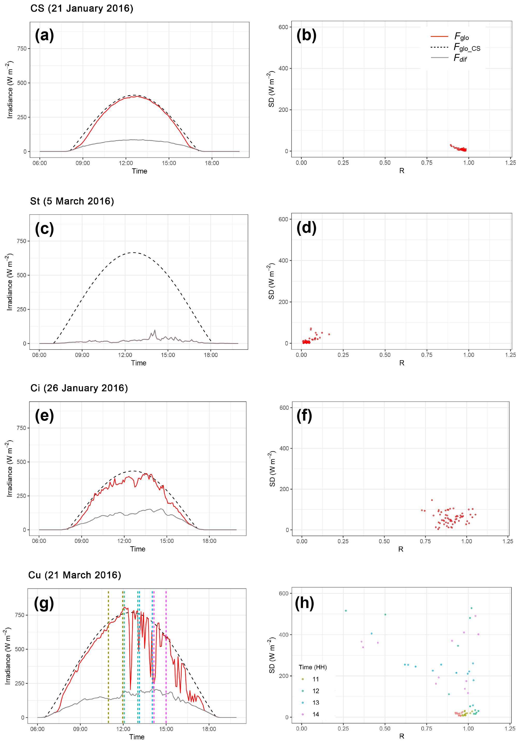
Figure 2Cloud classification based on broadband solar radiation following Duchon and O'Malley (1999). Each row represents a different cloud type on a specific day as a case study. The left column represents the time series of global and diffuse measured solar irradiance (Fglo and Fdif) and modelled clear-sky irradiance (Fglo_CS), while the right column contains the scatter SD–R plot of the observed SD of irradiance (SD) vs. the fraction of modelled clear-sky irradiance (R). In panel (h) different colours are related to different times (hours) of the day as reported in the legend.
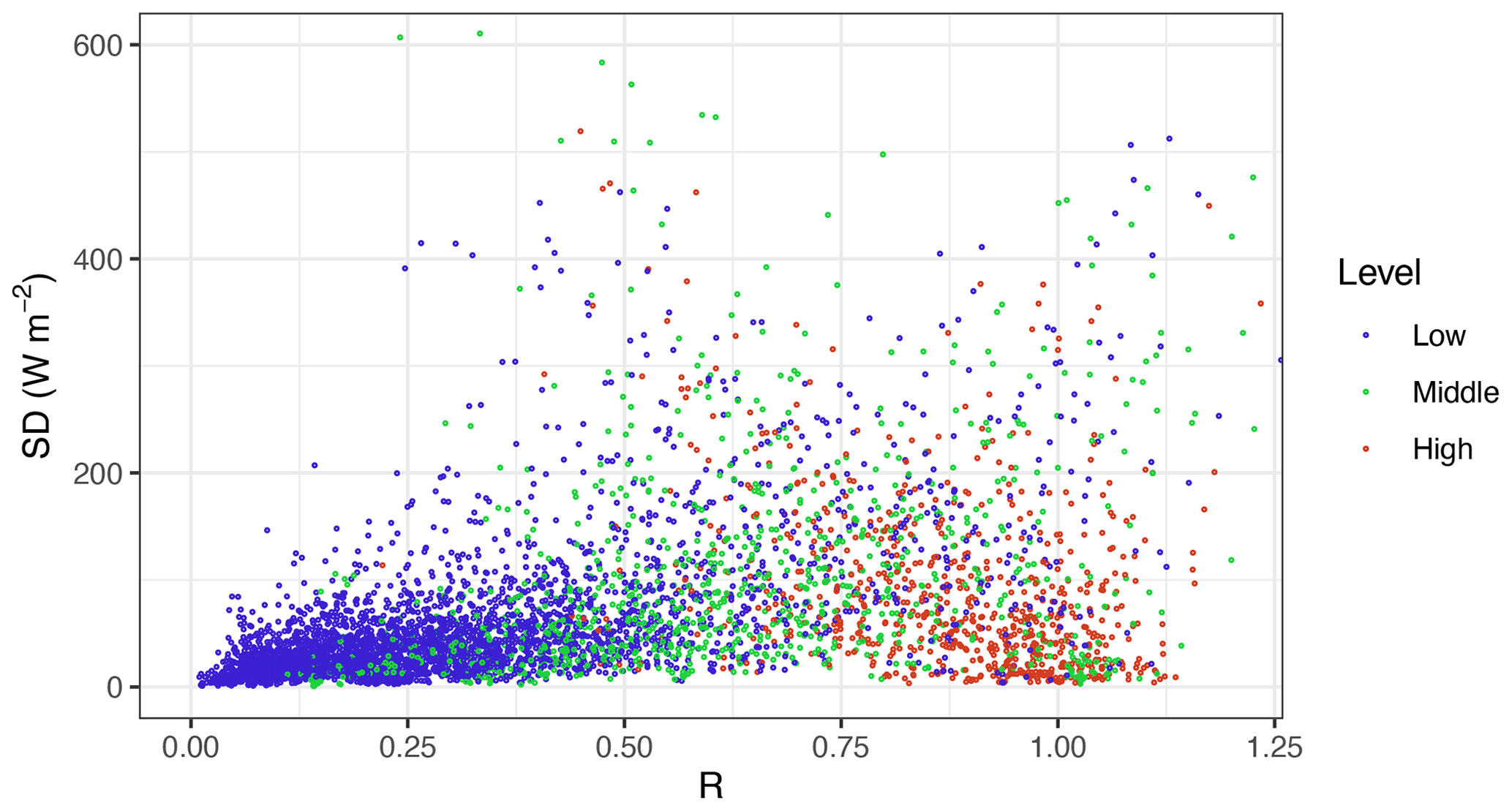
Figure 3SD–R plot of the whole dataset concerning the cloud base altitude grouped into three levels, namely low-level clouds (< 2 km), mid-altitude clouds (2–7 km) and high-altitude clouds (> 7 km).
Visualization of the SD vs. R (SD–R plot) results thus represents a first tool in distinguishing different cloud categories as a function of their efficiency in reducing the incoming solar radiation (R) and their persistency (SD). The potential of the SD–R plot is presented in Fig. 2a–h; it shows four examples of the temporal evolution of the observed Fglo, Fglo_CS andFdif (left column) and the corresponding SD–R diagrams (right column). Explored more in detail are the following:
-
The first case (Fig. 2a) shows Fglo following Fglo_CS without any significant temporal deviation, thus leading to a cluster of data in the SD–R diagram (Fig. 2b) characterized by R ∼ 1 and SD ∼ 0 W m−2. These conditions are those associated with clear-sky (CS) conditions by Duchon and O'Malley (1999).
-
The second case (Fig. 2c) shows Fglo completely dominated by the diffuse irradiance (Fdif) throughout the day (note that in Fig. 2c Fdif is superimposed on Fglo); this condition differs completely from the CS case, as both R and SD approach 0 (Fig. 2d). Duchon and O'Malley (1999) associate these conditions with the presence of persistent stratiform clouds.
-
The third case (Fig. 2e) reports Fglo approaching Fglo_CS and being at the same time characterized by small amplitude oscillations. In this case R ranges between 0.75 and 1, and SD ranges from 0 to ∼ 100 W m−2 (Fig. 2f). The cluster of data is thus more dispersed than that of the CS case featuring a larger variation in R and SD. Duchon and O'Malley (1999) attributed this situation to the presence of cirrus (Ci), underlining that in some borderline cases a misclassification between CS and Ci (just based on SD–R plot) could be possible.
-
The last case (Fig. 2g) represents a transition from a CS situation (before noon) to cloudy conditions (after midday) characterized by a significant scatter of Fglo. Figure 2h clearly shows that the sky condition evolves from the CS toward cloudy sky, shifting the R data from ∼ 1 down to ∼ 0.25 and increasing SD from ∼ 100 to ∼ 500 W m−2. According to Duchon and O'Malley (1999), the arrival of cumulus during a “good-weather” day could be the reason for such behaviour (Cu cloud movement in the sky results in fast sun–shadow transitions). Also, in this case, the SD–R plot alone cannot exclude the presence of other cloud types responsible for a similar behaviour (e.g. altocumulus, Ac; cirrocumulus, Cc; and cirrostratus, Cs). Note that in order to show the variation of data in the SD–R diagram (Fig. 2h) as a function of time, an hourly resolved colour code was assigned to the data points; the corresponding regions in Fig. 2g were delimited by dashed lines with the same colour code.
Overall, Fig. 2a–h shows the potential (and limits) of the SD–R plots for a preliminary broad sky–cloud classification. As mentioned, the SD–R diagram alone leaves margins of misclassification, especially because it is impossible to retrieve the required information when different cloud types at different levels are present simultaneously.
In the present work, we attempted a further refinement of cloud classification, including the information of the cloud base height (CBH) and the number of cloud layers obtained from the automated lidar–ceilometer measurements. The cloud base height is a key parameter in the characterization of clouds (Hirsch et al., 2011), since its estimation limits the number of potential cloud classes (that the SD–R classifier has to discriminate between), thus maximizing the efficiency of the Duchon and O'Malley (1999) classification algorithm. In fact, ceilometer instruments were developed and are commonly used in airports to operationally detect cloud layers, and their use for aerosol-related studies is more recent. Furthermore, the use of ceilometer data for cloud classification and cloud study purposes does not represent an absolute novelty in the scientific literature as demonstrated by recent works by Huertas-Tato et al. (2017) and Costa-Surós et al. (2013). The availability of CBH information allows for dividing cloud types in three fundamental categories (Tapakis and Charalambides, 2013): low-level clouds ( < 2 km), mid-altitude clouds (2–7 km) and high-altitude clouds ( > 7 km). From a general perspective the high-altitude cloud category includes cirrus (Ci), cirrocumulus (Cc) and cirrostratus (Cs); mid-altitude clouds include altocumulus (Ac), altostratus (As) and nimbostratus (Ns); low-level clouds include cumulus (Cu), stratocumulus (Sc), stratus (St) and cumulonimbus (Cb) (Tapakis and Charalambides, 2013; Ahrens, 2009; Cotton et al., 2011).
We colour-coded the SD–R diagram in Fig. 3 using the ceilometer-based information on cloud altitude. The plot shows that, on average, low-level clouds are located on the left side of the SD–R diagram (stratiform clouds), while high-altitude clouds are conversely on the opposite side (Ci and Cu clouds); finally, mid-altitude clouds mostly cover the central part, describing all the possible transitions and combinations from St to Cu and Ci, e.g. altostratus (As) and altocumulus (Ac).
Overall, adding the CBH information to the SD–R plot enabled us to identify eight cloud types: St (stratus), Cu (cumulus) and Sc (stratocumulus) as low-level clouds; As (altostratus) and Ac (altocumulus) as mid-altitude clouds; Ci (cirrus) and Cc–Cs (cirrocumulus and cirrostratus merged in one single class) as high-altitude clouds.
Table 1Final criteria adopted for cloud classification. SD represents the SD of the measured global irradiance with respect to the theoretical behaviour in clear-sky conditions; R represents the ratio between observed global irradiance (Fglo) and the modelled irradiance (Fglo_CS) in clear-sky conditions; and finally the cloud layer is the number of cloud layers detected by the lidar.

A summary of the threshold values of R, SD and cloud level used here to the final cloud classification is given in Table 1, with the R and SD limits being based on the works of Duchon and O'Malley (1999) and Harrison et al. (2008) and those of the CBH being derived considering the cloud properties at midlatitudes.

Figure 4Cloud classification based on the improved broadband solar radiation following Duchon and O'Malley (1999) and Harrison et al. (2008) coupled with lidar data of cloud base height. From left to right: stratus (St), altostratus (As), stratocumulus (Sc), altocumulus (Ac), cirrocumulus and cirrostratus (Cc–Cs), cumulus (Cu), cirrus (Ci), and finally clear-sky (CS) conditions. The SD–R plot reports in grey the single data of the whole dataset, while centroids and the 99 % confidence interval of each cloud type are plotted in a colour scale related to the cloud base level.
Finally, to avoid misclassification due to the presence of multiple cloud layers, the analysis was limited to those cases where only one cloud layer was detected by the ceilometer (8405 single layer cases, representing 61 % of all measurements). Another reason for limiting the analyses to one cloud layer is due to the main aim of this work: to quantify the effects of different cloudiness and cloud types on the LAA HR. We wanted to avoid conditions with multiple-layer clouds, as this would result in confounding information for the purpose of the present study.
Figure 4 shows the SD–R diagram of all data (grey) with superimposed R and SD mean values and a 99 % confidence interval for each of the eight identified cloud classes, plus clear-sky (CS) conditions. The final cloud classification was obtained for the period from November 2015 to March 2016, during which all necessary parameters were available (Sect. 3).
Since this methodology is applied for the first time in the Po Valley, a complete validation of the aforementioned approach is reported in Appendix B (“Cloud type validation”). It includes two validation exercises: the first was carried out comparing the present automatized cloud classification with a visual cloud classification based on sky images collected during 1 month of the wintertime field campaign; the second was carried out comparing the present automatized cloud classification with the one discussed by Ylivinkka et al. (2020). In fact, simultaneously to the submission of our work, Ylivinkka et al. (2020) proposed a classification based on the coupling of irradiance and CBH measurements. Overall, based on these comparisons, agreement with our classification is 80 % with the visual approach and 90 % with the Ylivinkka et al. (2020) methodology, with these results further demonstrating the reliability of the cloud classification algorithm used in our study.
Data measured over Milan from November 2015 to March 2016 are presented in Sect. 3.1, with this period covering the simultaneous presence of radiation, lidar–ceilometer and absorption information necessary for the analysis. The role of cloudiness and cloud type on the total HR is discussed in Sect. 3.2; the impact of clouds on the HR is discussed with respect to the light-absorbing aerosol species, BC and BrC, in Sect. 3.3. All data are reported as the mean ± 95 % confidence interval.
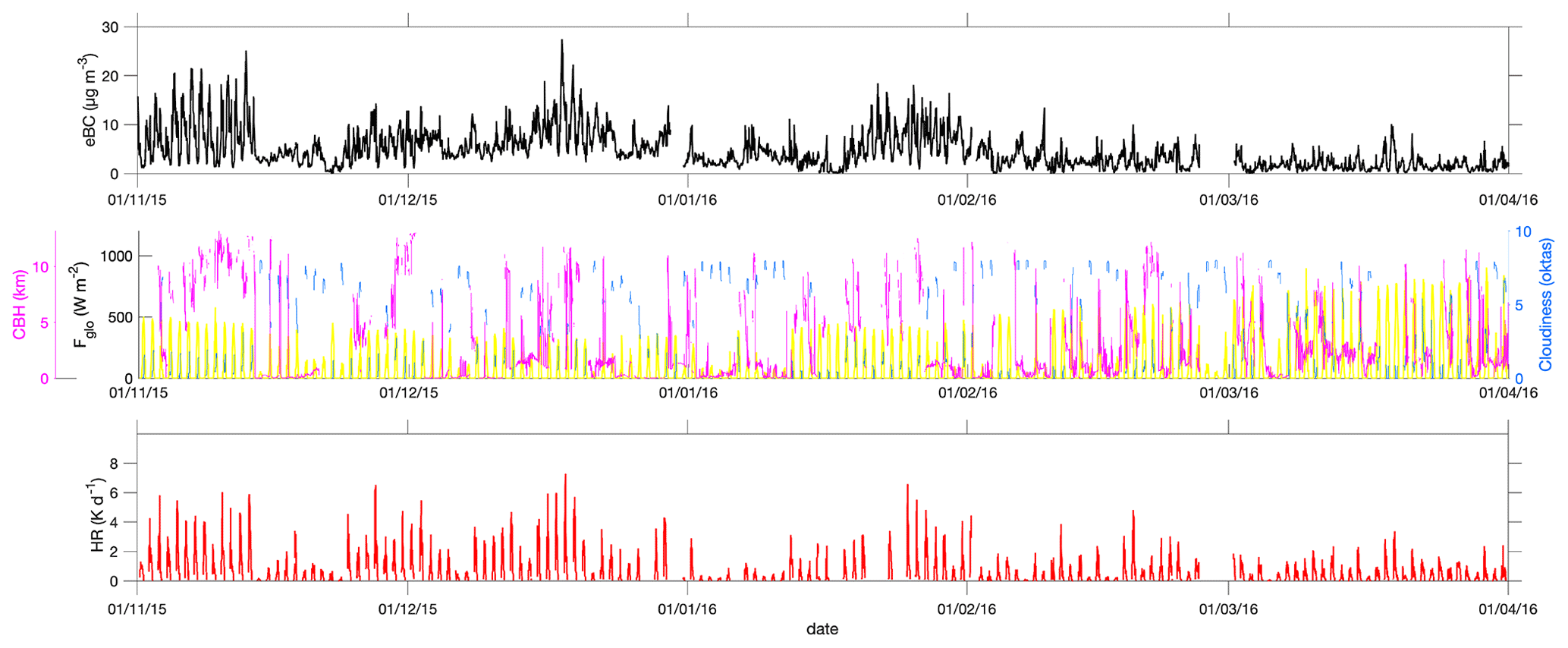
Figure 5High-time-resolution data (5 min) for eBC, global irradiance (Fglo, yellow line) cloud base height (CBH), cloudiness (oktas) and the related heating rate (HR) from 1 November 2015 to 1 April 2016.
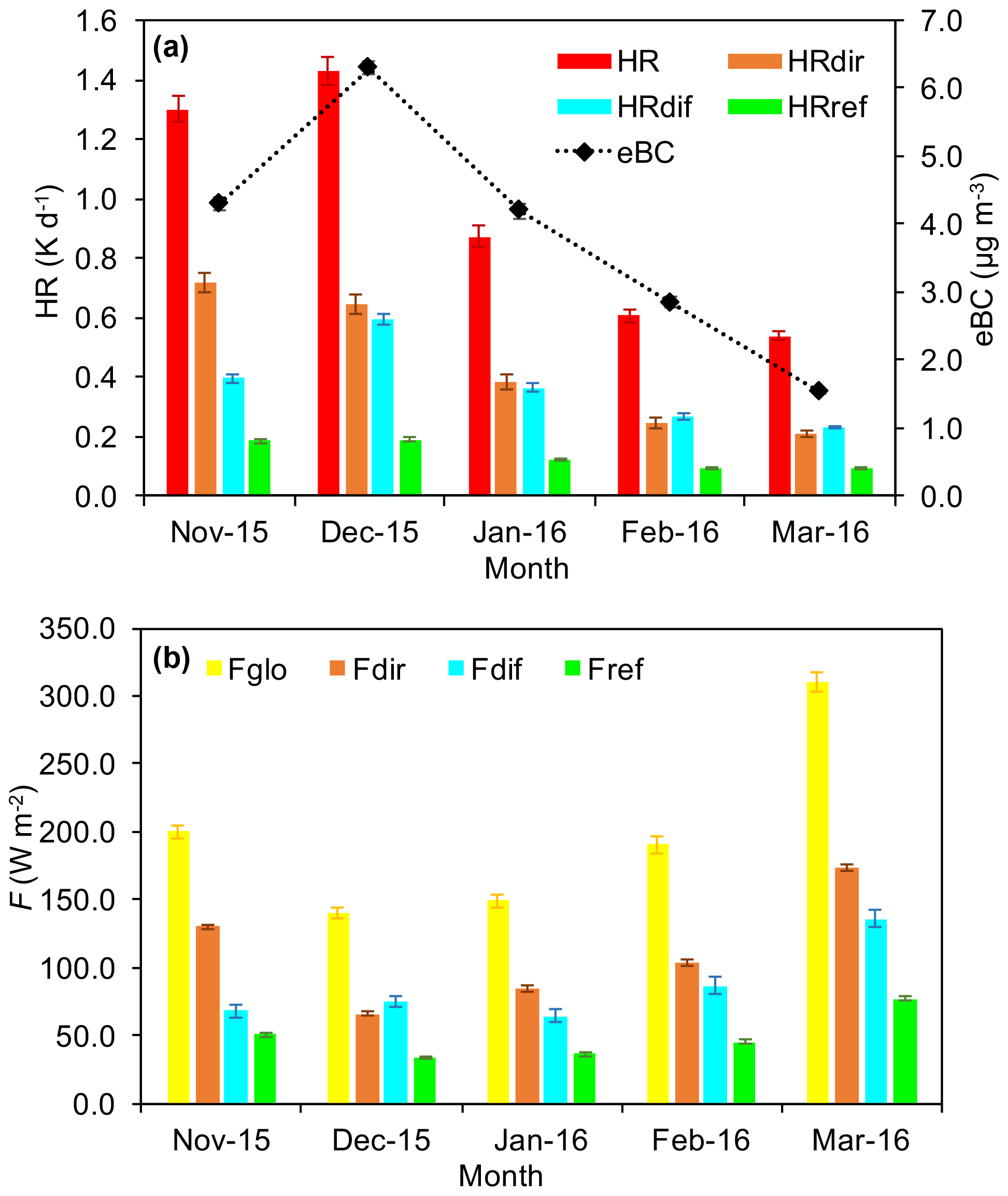
Figure 6Monthly averaged values of (a) eBC and HR values and their direct, diffuse and reflected components (HRdir, HRdif and HRref); (b) global radiation values (Fglo) and their direct, diffuse and reflected components (Fdir,Fdif and Fref).
Table 2Monthly averaged data and the confidence interval at 95 % of temperature (T), pressure (P), equivalent black carbon (eBC), absorption coefficient (babs) and heating rate (HR) divided into their direct (dir), diffuse (dif) and reflected (ref) components and, finally, global (Fglo), direct (Fdir), diffuse (Fdif) and reflected (Fref) irradiances.
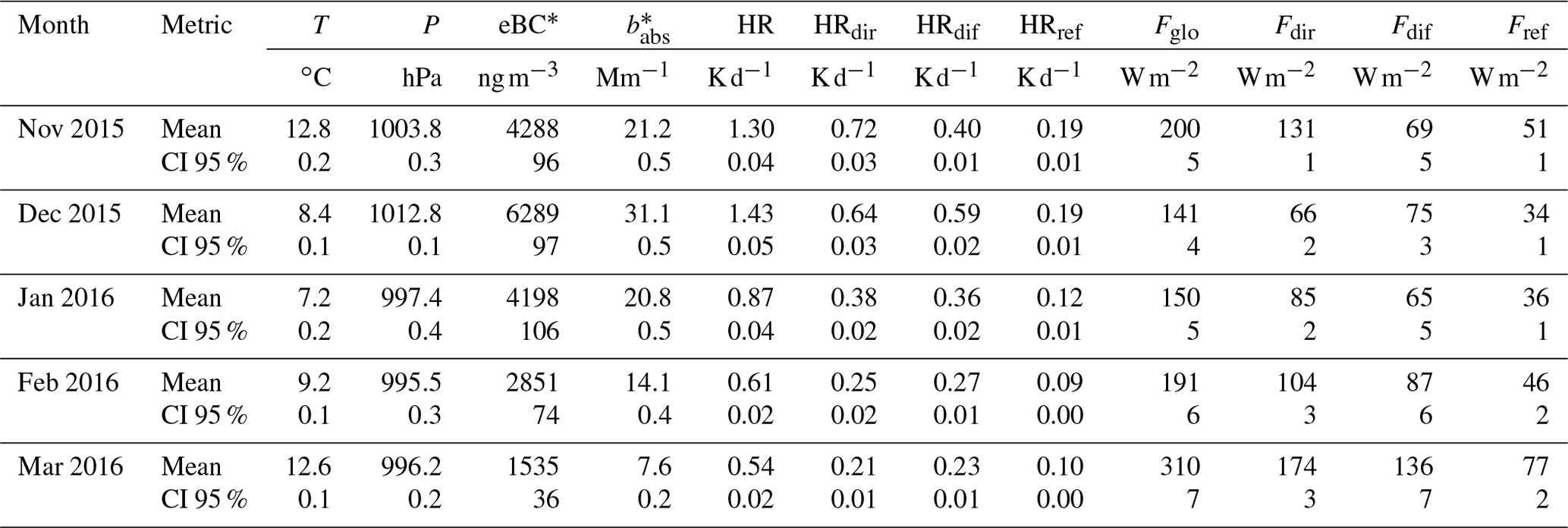
* denotes aethalometer data referring to λ = 880 nm.
3.1 eBC, irradiance, HR and cloud data presentation
Highly time-resolved data (5 min) of eBC, Fglo, CBH, cloudiness (oktas) and the resulting HR are shown in Fig. 5; their monthly average values are presented in Fig. 6a and summarized in Table 2.
The lower eBC and babs (880 nm) values (monthly averages of 1.54 ± 0.04 µg m−3 and 7.6 ± 0.2 Mm−1) were recorded in March, while their higher values were found in December (6.29 ± 0.09 µg m−3 and 31.1 ± 0.5 Mm−1, respectively) with a maximum value of 27.44 µg m−3 (135.7 Mm−1). In December, the average PM10 and PM2.5 were also at their maximum, with 73.1 ± 0.6 and 69.3 ± 0.6 µg m−3, respectively (source: Milan Environmental Protection Agency, ARPA Lombardia, https://www.arpalombardia.it/Pages/Aria/Richiesta-Dati.aspx, last access: 25 March 2021), and the eBC accounted for ∼ 10 % of PM mass concentration. These high values of eBC and PM10 and PM2.5 agree with those observed previously in wintertime in the Po Valley, when strong emissions in the Po Valley are released into a stable boundary layer (Sandrini et al., 2014; Ferrero et al., 2011b, 2014, 2018; Barnaba et al., 2010). During the investigated period, the lower monthly irradiance value was observed in December (Fglo of 141 ± 4 W m−2; Table 2), while the higher value was in March (Fglo of 310 ± 7 W m−2). The higher monthly average HR was recorded in December (1.43 ± 0.05 K d−1), while the lower one was in March (0.54 ± 0.02 K d−1; see Fig. 6a and Table 2). Even though the HR monthly behaviour is correlated with eBC (Table 2; R2 = 0.82, not shown), it is also useful to compare the maximum-to-minimum ratio of the eBC monthly mean (December to March, eBC ratio of 4.10 ± 0.12) to the same for the HR (2.65 ± 0.16). This ratio is higher for eBC because the incoming irradiance was lower in December (Fglo of 141 ± 4 W m−2; Fig. 6b) with respect to March (Fglo of 310 ± 7 W m−2, ratio of 0.45 ± 0.02), partially compensating the marked wintertime increase of eBC. This is due to the interaction of LAA with Fdir. In fact, once Fdir is scaled by cos (θz) (Eq. 3, Sect. 2.2, Fig. S4 in the Supplement) it is quite constant throughout the year (and perfectly constant only in clear-sky conditions). Conversely, the diffuse and reflected irradiance, under the isotropic and Lambertian assumptions (Eq. 3), remain seasonally modulated (Fig. S4).
These observations illustrate the importance of both the amount and the type (direct, diffuse and reflected) of radiation that interacts with LAA. In brief, any process able to influence the total amount and the type of impinging irradiance (e.g. presence or absence of clouds, cloudiness, and cloud type) will result in a different HR, even at constant LAA concentrations (and their absorption). The investigation of this aspect is the main focus and added value of this study. High-resolution data (Figs. 5 and S4) provided a first hint to the importance of cloud presence on the HR; a sharp global irradiance decrease was observed in cloudy conditions, especially in the presence of low-level clouds (low CBH) and high cloud cover (7–8 oktas).
Thus, both cloudiness and cloud type were carefully determined as detailed in Sect. 2.3.1 and 2.3.2. Overall, during the whole campaign, the average cloudiness was 3.58 ± 0.04 oktas with the higher monthly value in February (4.56 ± 0.07 oktas) and the lower one in November (2.91 ± 0.06 oktas). These data are in line with the mean cloudiness over Europe (∼ 5.5 oktas; Stjern et al., 2009) and over Italy (∼ 4 oktas; Maugeri et al., 2001). Moreover, during the campaign, clear-sky (CS) conditions were only present 23 % of the time, with the remaining time (77 %) being characterized by partially cloudy (35 %, 1–6 oktas) to totally cloudy (42 %, 7–8 oktas) conditions.
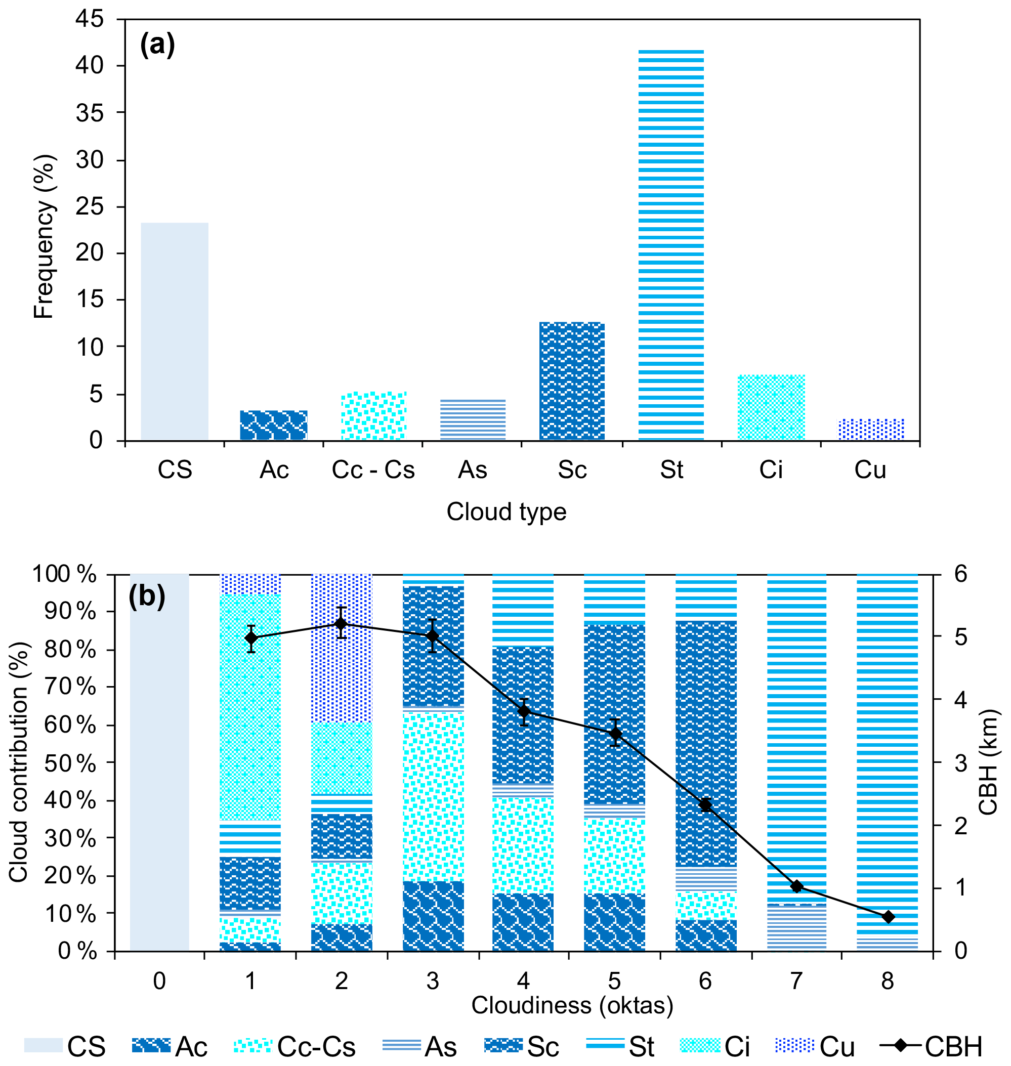
Figure 7(a) Time frequency (%) of the cloud type classified over the U9 site (CS means clear-sky conditions); (b) contribution (%) of each cloud type to the okta values measured over the U9 site.
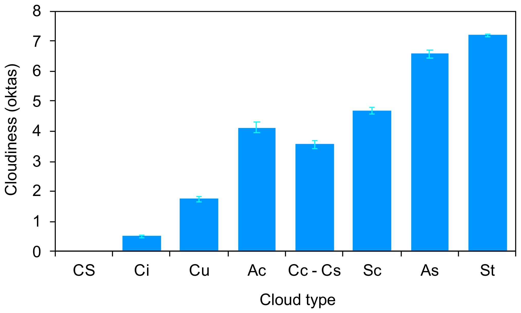
Cloudy conditions are therefore frequent. The frequency of specific cloud type occurrence is given in Fig. 7a. The dominating cloud type was St (42 %), followed by Sc (13 %), Ci and Cc–Cs (7 % and 5 %, respectively). The contribution of each cloud type to the cloudiness is reported in Fig. 7b. While St clouds were mostly responsible for overcast situations (7–8 oktas, frequency of 87 % and 96 %), Sc clouds dominated the intermediate cloudiness conditions (5–6 oktas, frequency of 47 % and 66 %), and the transition from Cc–Cs to Sc determined moderate cloudiness (3–4 oktas). Finally, low cloudiness values (1–2 oktas) were mostly dominated by Ci and Cu (frequency of 59 % and 40 %, respectively). As mentioned (Sect. 2.3.2 and Fig. 4), low-level clouds ( < 2 km) include stratus (St), cumulus (Cu) and stratocumulus (Sc); mid-altitude clouds (2–7 km) include altostratus (As) and altocumulus (Ac); and high-altitude clouds ( > 7 km) include cirrus (Ci), cirrocumulus and cirrostratus (Cc–Cs). Thus, it is clear that the higher cloud cover (higher okta value) is due to a higher frequency of low–mid-altitude clouds. This is evident in Fig. 7b, which reports the average CBH for each okta. The CBH was related to oktas (Fig. S5a in the Supplement), underling the linkage (together with Fig. 7b) between the fraction of the sky covered by clouds and the cloud type responsible for it, at least at the measuring site. Indeed, the cloudiness is a non-linear function of the cloud type, as cloud types are related to the meteorological patterns; e.g. highly persistent stratiform clouds generate cloudy weather in conditions with lower wind (see the Supplement for further details). Figure 8 summarizes the average cloudiness associated with different cloud types showing an okta rise from conditions dominated by cirrus clouds (0.51 ± 0.05 oktas) to stratus clouds (7.20 ± 0.04 oktas). This is in agreement with the recent work of Bartoszek et al. (2020), who associated a higher cloudiness level with the presence of stratiform clouds. The possible role of wind on cloud type is explored in Fig. S6 in the Supplement (“Wind speed, cloudiness and clouds”).
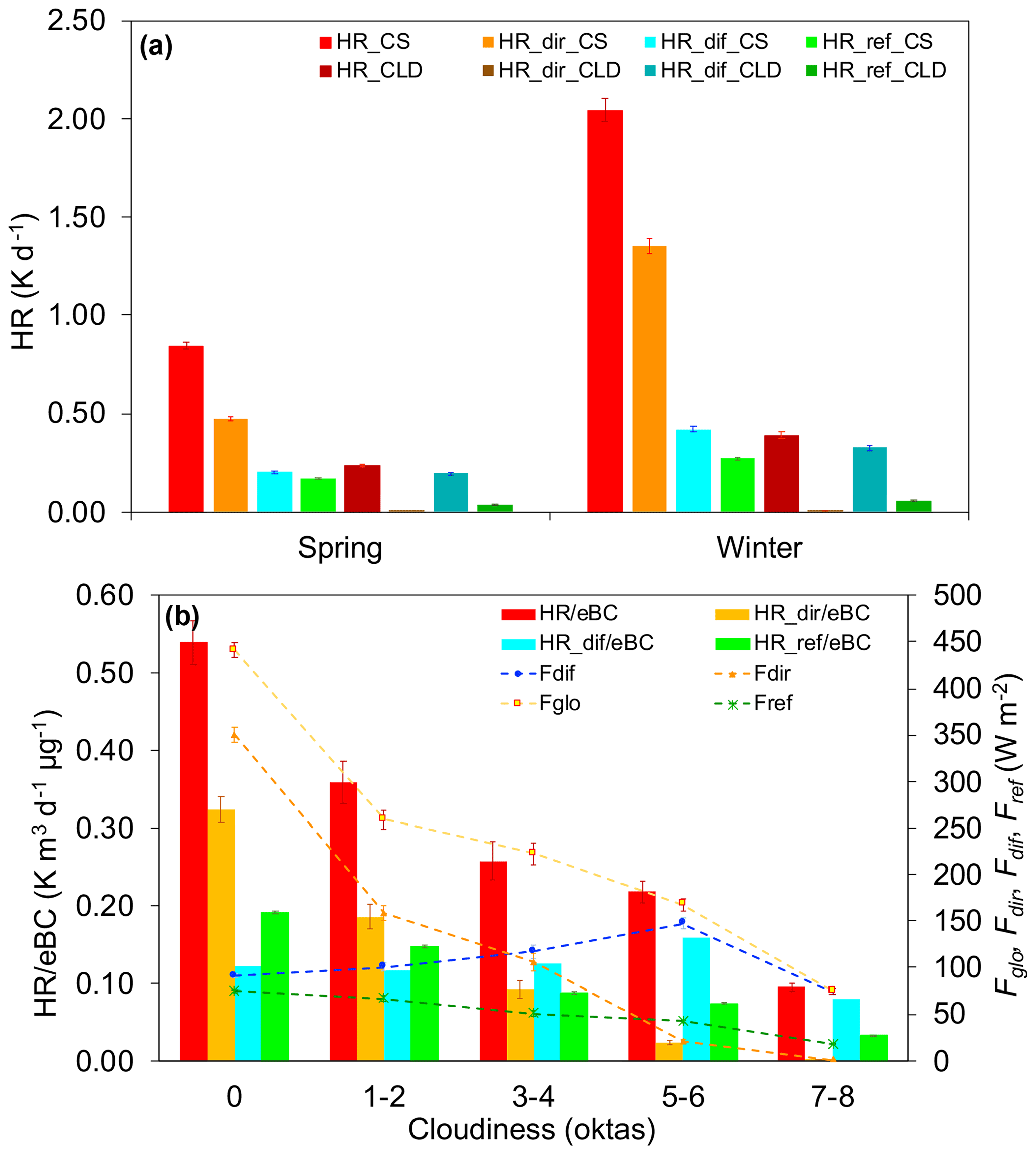
Figure 9Monthly averaged values of (a) HR values and their direct, diffuse and reflected components (HRdir, HRdif and HRref) during winter and spring both in clear-sky (CS; 0 oktas) and cloudy (CLD; 7–8 oktas) conditions. (b) values together with their direct, diffuse and reflected components (, and ); the direct, diffuse and reflected irradiance (Fdir, Fdir and Fdif); and the global irradiance (Fglo).
3.2 Cloud impact on the heating rate
3.2.1 The role of cloudiness
Figure 6a already provided the first indication of the important influence of clouds on the total HR. In fact, it shows the magnitude of the absolute (and relative) contribution of the diffuse component (HRdif) with respect to the total HR revealing that, on a monthly basis, the diffuse contribution accounted on average for 40 ± 1 % (of the total HR). In most cases this was comparable or even higher than the HRdir. The only exception was in November 2015 when the lower HRdif (Fig. 6a) and Fdif (Fig. 6b) fractions in the total HR and Fglo were measured (30.4 ± 1.4 % and 34.3 ± 2.6 % of the total, respectively), with this also being the month with the lowest average cloudiness (2.91 ± 0.06 oktas). The aforementioned data demonstrate the importance of the diffuse component of radiation. Therefore, the absolute values of the HR and its components were firstly investigated as a function of cloudiness (clear-sky and completely overcast situations, seasonal averages, Fig. 9a). In the wintertime clear sky, the direct component of the HR (HRdir) was higher than the HRdif and HRref, accounting for 1.35 ± 0.04 K d−1 and explaining on average 60 ± 5 % of the total HR. Similarly, in the springtime clear sky, HRdir was 0.47 ± 0.01 K d−1, again higher than the HRdif and HRref. Conversely, in a completely overcast condition (7–8 oktas), the HRdif dominated (84 ± 1 % of the total HR) and accounted for 0.33 ± 0.01 and for 0.19 ± 0.01 K d−1 during winter and spring, respectively.
In order to further investigate the role of cloudiness, we decoupled the variability of the HR induced by radiation from that due to LAA concentrations. Thus, the HR values and those of its components (HRdir, HRdif and HRref) were normalized to the unit mass of eBC () and reported as a function of cloudiness in Fig. 9b together with the measured irradiance (Fglo, Fdir, Fdif and Fref): this parameter () reports the efficiency of warming per mass concentration of eBC at different cloudiness levels. Overall, Fig. 9b shows the general decease of for increasing cloud cover, a pattern also observed for both and , which follow the respective decrease of direct and reflected irradiance. Note that at okta values of 7–8, reached values close to 0 (due to the suppression of Fdir by clouds), while was 0.03 ± 3 × 10⁻⁴ due to the presence of surficial albedo effect on the diffuse irradiance (Fdif). increased with increasing cloudiness up to intermediate cloudiness conditions (5–6 oktas), reaching a maximum (0.16 ± 0.01 ). This is in line with the behaviour of the diffuse irradiance: maximum of 147 ± 6 W m−2 (at 5–6 oktas), doubling the value in overcast conditions (74 ± 3 W m−2; 7–8 oktas) and exceeding 150 % of that for clear-sky conditions (91 ± 2 W m−2). In the overcast condition (7–8 oktas) both and the diffuse irradiance reached their minimum due to the capability of clouds to effectively attenuate the incoming radiation. However, in these conditions, was still not null (0.08 ± 0.01 ), dominating the total atmospheric HR, with a contribution of 84 ± 1 %.
and cloudiness data were linearly related, showing a high level of correlation (R2 = 0.935, Fig. S5b). Cloudiness could thus be used as good predictor (in modelling activity) for .
As from Fig. S5a (Sect. 3.1), the CBH appeared related to the cloudiness, and an additional linear correlation was tested between and the CBH (Fig. S5c; R2 = 0.857); this relationship is weaker than that between and cloudiness. Cloudiness, describing the fraction of sky covered by clouds, is a better predictor of the capability to suppress the incoming radiation (and thus the HR promoted by LAA). The relationship between the CBH and cloudiness should be also investigated in other monitoring sites around the world to explore the possibility of using the CBH (together with cloudiness) as a promising prognostic variable for the HR of LAA in future studies.

Figure 10Diurnal pattern of eBC (a), wind speed (b), global irradiance (Fglo) (c) and HR (d). Data are averaged for clear-sky conditions (CS; 0 oktas) and cloudy conditions (CLD; 7–8 oktas).
Overall, our experimental HR data enabled us to estimate the degree of error introduced by improperly assuming clear-sky conditions in radiative-transfer calculations. Particularly, we found that the simplified assumption of clear-sky conditions leads to an overestimation of the LAA-induced HR by a factor ranging from 50 % to 470 % (50 % in low cloudiness: 1–2 oktas; 109 % in moderate cloudiness: 3–4 oktas; 148 % in intermediate cloudiness: 5–6 oktas; and 470 % in cloudy conditions: 7–8 oktas). These results clearly highlight that clouds are responsible for an important feedback on the aerosol HR that needs to be carefully quantified, pointing to the need to correctly include and model cloudy conditions in radiative-transfer calculations aimed at evaluating the real contribution of aerosol forcing on the atmospheric HR on a global scale.
3.2.2 Cloudiness and diurnal pattern of the HR
The presence of clouds can also alter the HR diurnal pattern. Figure 10a–d show the mean diurnal pattern of eBC, wind speed, Fglo and the HR in both clear-sky (0 oktas) and cloudy conditions (7–8 oktas). In clear-sky conditions, the eBC peaked at 08:00 LST (6.41 ± 0.31 µg m−3) during the rush hour (Fig. 10a); then eBC decreased until its minimum in the early afternoon (1.07 ± 0.10 µg m−3) when the wind speed reached its maximum (1.5 ± 0.1 m s−1, Fig. 10b). The incoming Fglo in clear-sky conditions peaked as expected at midday with 497 ± 10 W m−2 (Fig. 10c). This caused an asymmetric HR diurnal pattern, being characterized by a fast increase to the maximum at 10:00 LST (3.60 ± 0.18 K d−1) and a subsequent slower decrease by sunset (Fig. 10d). This pattern was not present in cloudy conditions (Fig. 10d). First, eBC showed a moderate peak at 10:00 LST (4.09 ± 0.20 µg m−3) being quite stable during the afternoon – remaining above 3 µg m−3 until 16:00 LST (Fig. 10a). The eBC behaviour was consistent with that of wind speed, which only slightly rose during the day but was however always below 1 m s−1 (on average 0.64 ± 0.03 m s−1, Fig. 10b). The incoming Fglo in cloudy conditions peaked again as expected at midday with 103 ± 4 W m−2 with a much slower increase during the day (Fig. 10c). The Supplement (“Wind speed, cloudiness and clouds”) and Fig. 7b show that cloudy conditions were mostly associated with stratus and very low windy conditions (0.64 ± 0.02 m s−1), explaining the flat diurnal behaviour of eBC differing from the clear-sky case. Moreover, the absence of any direct irradiance in cloudy conditions (Fig. 9b; Sect. 3.1) determines that Fglo was essentially due to the diffuse irradiance whose symmetrical bell-shaped curve drove the HR behaviour (Fig. 10d), peaking at midday with a value of 0.74 ± 0.01 K d−1 (much lower than in CS).

Figure 11Impact of each cloud type on the heating rate normalized to black carbon concentration: (a) and Fglo, (b) and Fdir, (c) and Fdif, and (d) and Fref.
As a conclusion, in different cloudiness conditions, not only the absolute magnitude of the HR but also its diurnal pattern are different. This also changes the related atmospheric feedbacks, such as the influence on the liquid water content (Jacobson, 2002), planetary boundary layer dynamics (Wang et al., 2018; Ferrero et al., 2014), regional circulation systems (Ramanathan and Feng, 2009; Ramanathan and Carmichael, 2008), and finally the cloud dynamic and evolution itself (Koren et al., 2008; Bond et al., 2013). Thus, an inappropriate use of the clear-sky assumption in models will also reflect on the modelled HR-triggered feedbacks. These results also acquire relevance in the context of the counterintuitive semi-direct effect proposed by Perlwitz and Miller (2010) and referred to in Sect. 1: the atmospheric heating induced by tropospheric absorbing aerosol could lead to a cloud cover increase (especially low-level clouds). Such a feedback stresses the need for a proper inclusion of sky conditions into radiative-transfer calculations.
3.2.3 The role of cloud type
The previous sections showed the effect of cloudiness on the total LAA HR. The impact of each cloud type on the HR is addressed here, as not all clouds have the same effect on irradiance (Tapakis and Charalambides, 2013). As previously done, we refer to HR values normalized to eBC unit mass () to decouple radiation and aerosol effects. Figure 11a–d show the total and Fglo together with the corresponding components ( and Fdir, and Fdif, and and Fref; Fig. 11b–d). The figure shows a prefect agreement between cloud type, irradiance and the corresponding component (R2 > 0.93; not shown). It also highlights how critical it is, for radiative-transfer calculations and HR determination, to take into account the role of each cloud type. Only the cloud influence on the is markedly different from the other components.

Figure 12Average values of the total HR, HRdir, HRdif and HRref as a function of the cloud type.
In terms of absolute values (not normalized for eBC), Fig. 12 reveals that the HRdir was only dominant during periods of CS and Ci clouds (HRdir of 1.11 ± 0.04 and 0.92 ± 0.05 K d−1, respectively), explaining 66 ± 3 % and 57 ± 4 % of the total atmospheric HR. In the cases of other clouds (St, As and Sc) HRdif dominates, reaching the highest absolute contribution of 84.4 ± 3.8 %, 83.0 ± 10.7 % and 76 ± 4 % (HRdif of 0.25 ± 0.01, 0.34 ± 0.03 and 0.66 ± 0.02 K d−1), respectively.

Figure 13Percentage decrease of the HR with respect to clear-sky conditions as a function of the cloudiness (oktas) averaged for each cloud type.
Given this impact of cloud type, the ability of cloudiness to be a good predictor for the HR (as detailed in Sect. 3.2.1), and the relationship (over the investigated site) between cloudiness and cloud type (Sect. 3.1, Fig. 7b), the synergic impact of cloudiness and cloud type on the HR was investigated and presented in Fig. 13. In the figure, we summarize the HR results in terms of percent difference from the clear-sky (CS) case by averaging the cloudiness (in oktas) for each cloud type (as detected in Sect. 3.3). Overall, the derived linear regression indicates an HR decrease of −11.9 ± 1.2 % per okta. The regression R2 (0.963) was slightly higher than that reported in Fig. S5b (R2 = 0.935; relationship with the cloudiness only) suggesting the need (for precise calculations) to account for the cloud types responsible for any sky coverage in agreement with a recent work of Bartoszek et al. (2020). Figure 13 also allowed us to associate the HR decrease with each specific cloud type over Milan. Particularly, Ci clouds produced a modest impact on cloudiness (0.50 ± 0.05 oktas), decreasing the HR by ∼ 3 %, while Cu clouds (1.76 ± 0.09 oktas) decreased the HR by −26 ± 8 %. Cc–Cs clouds (3.56 ± 0.14 oktas) were responsible for a −49 ± 6 % decrease of the HR. Their impact was comparable to that of Sc clouds (4.68 ± 0.10 oktas, −48 ± 4 % of the HR). Ac clouds (4.11 ± 0.18 oktas) had a higher impact, decreasing the HR by −59 ± 6 %. The highest impact was due to As (6.57 ± 0.15 oktas; −76 ± 4 % of the HR) and by St (7.19 ± 0.04 oktas) that suppressed the HR by a factor of −83 ± 4 %.
3.3 The impact of clouds on the BC and BrC heating rates
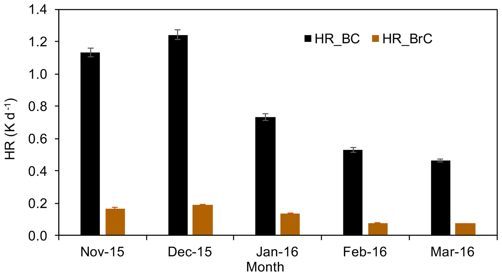
In this last part of the work we focus on the HR of the two main absorbing aerosol species: BC and BrC (obtained as detailed in Sect. 2.1.1). The monthly averaged values of the HR of BC and BrC (HRBC and HRBrC) are reported in Fig. 14. The highest HRBC and HRBrC values were recorded in December (1.24 ± 0.03 K d−1 and 0.19 ± 0.01 K d−1), while the lowest were recorded in March (0.46 ± 0.01 K d−1 and 0.07 ± 0.01 K d−1). Overall, the HRBrC accounted for 13.7 ± 0.2 % of the total HR.
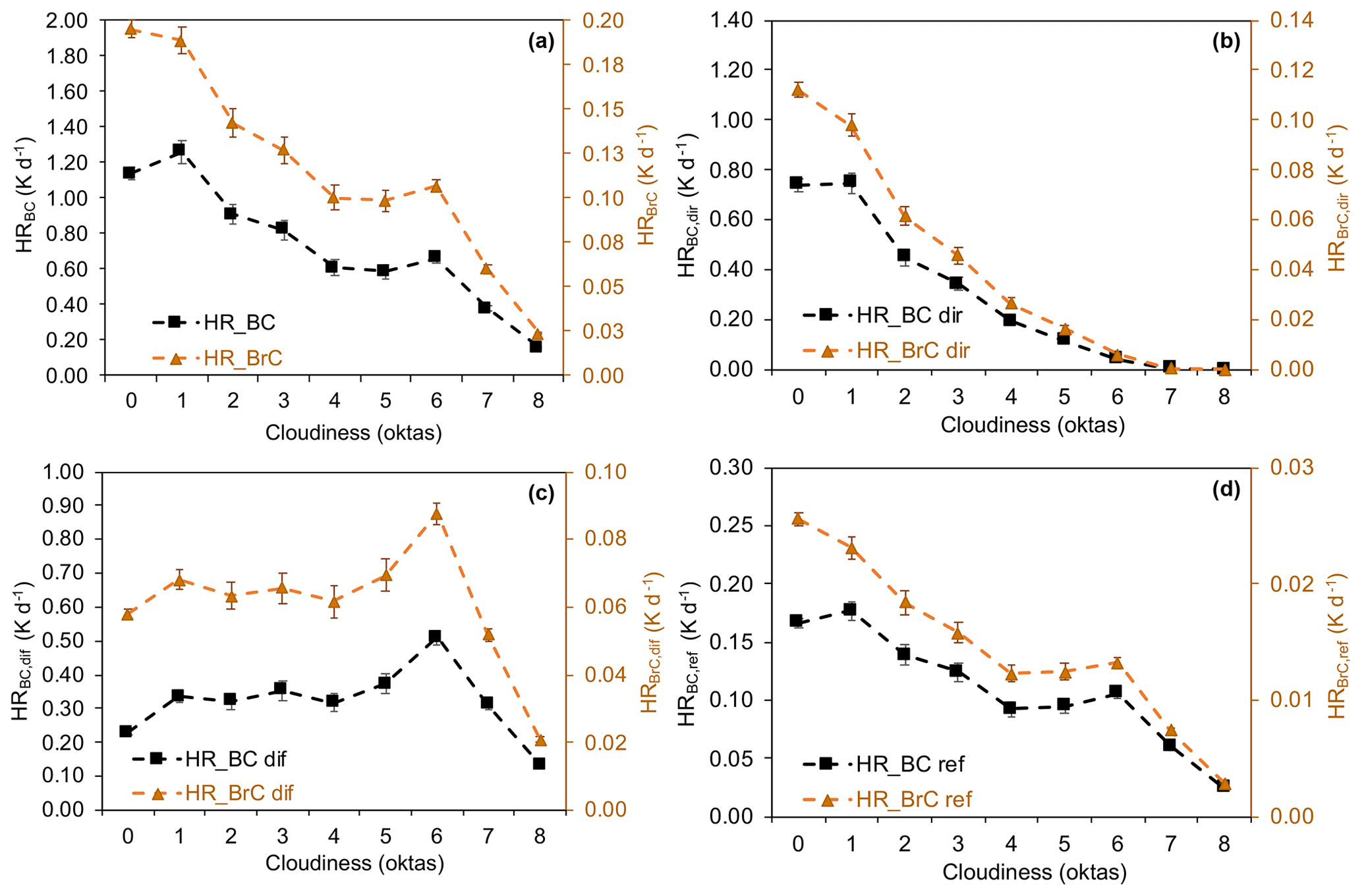
Figure 15The HR of BC and BrC as a function of the cloudiness (oktas): (a) total HRBC and HRBrC, (b) direct component of both the HRBC and HRBrC (HRBC,dir and HRBrC,dir), (c) diffuse component of both the HRBC and HRBrC (HRBC,dif and HRBrC,dif), and (d) reflected component of both the HRBC and HRBrC (HRBC,ref and HRBrC,ref). Note that, due to the different magnitude of the HRBC and HRBrC, the y axis of the HRBrC in the four panels was chosen as of that of the HRBC.
The variability of the total HRBC and HRBrC as a function of cloudiness is reported in Fig. 15a, with panels b–d showing their direct (HRBC,dir and HRBrC,dir), diffuse (HRBC,dif and HRBrC,dif) and reflected (HRBC,ref and HRBrC,ref) components. Figure 15a shows that both the HRBC and HRBrC decreased with increasing cloudiness, going from the CS maxima (HRBC and HRBrC of 1.14 ± 0.03 and 0.20 ± 0.01 K d−1) to the completely overcast condition minima of 0.16 ± 0.01 and 0.02 ± 10−3 K d−1 (8 oktas; mainly due to St and As clouds; see Fig. 7b). As shown in Fig. 9b, the change of irradiance magnitude with cloudiness was different for direct, diffuse and reflected components affecting the corresponding direct, diffuse and reflected components of the HRBC and HRBrC (Fig. 15b–d). The HRBC,dir and HRBrC,dir (Fig. 15b) decreased as a function of cloudiness from 0.74 ± 0.03 and 0.11 ± 0.01 K d−1 (0 oktas) to negligible levels (HR < 10−4 K d−1) in completely overcast conditions. The HRBC,dif and HRBrC,dif (Fig. 15c) increased with cloudiness, reaching their maximum in partially cloudy conditions (at 6 oktas: 0.51 ± 0.01 and 0.09 ± 0.01 K d−1). Further increasing cloudiness reduced their values to minimum values (0.13 ± 0.01 and 0.02 ± 0.01 K d−1). The HRBC,ref and HRBrC,ref (Fig. 15d) behave similarly to the total HRBC and HRBrC, since the reflected irradiance is dominated by the global irradiance impinging on the ground (see Fig. 9b for a comparison); the HRBC,ref and HRBrC,ref decreased with increasing okta values from maximum values in clear-sky conditions (HRBC,ref and HRBrC,ref of 0.17 ± 4 × 10⁻³ and 0.03 ± 1 × 10⁻³ K d−1) down to the overcast minimum (HRBC,ref and HRBrC,ref of 0.02 ± 10−3 and 3 × 10⁻³ ± 10−3 K d−1). Figure 15a–d also show that the HRBC was always greater (in absolute values) than the HRBrC, as expected. The relative decrease of the HRBrC from CS to completely overcast conditions was 12 ± 6 % larger with respect to that of the HRBC. At a first glance, Fig. 15a–d could give the impression that BrC is more efficient in heating the surrounding atmosphere (with respect to BC) in CS conditions. However, any change of both BC and BrC babs(λ) in different sky conditions has to be taken into account to avoid any misinterpretation of the results. While the variability of BC babs(λ) with cloudiness was limited (with the exception of 1 okta, Fig. S7a in the Supplement), this was not the case for BrC. In fact, babs(λ) BrC values in high cloudiness were statistically lower than the ones in CS conditions (at 8 oktas, babs(λ) of BrC was −23 ± 3 % lower than in CS conditions, Fig. S7b). The relative decrease of the HRBrC with cloudiness was therefore higher compared to that of the HRBC. Understanding of the reason behind the observation of higher babs(λ) values for BrC in CS conditions is beyond the aim of the present paper (we can speculate that it could be related to the formation of secondary BrC at high radiation levels; e.g. Kumar et al., 2018).
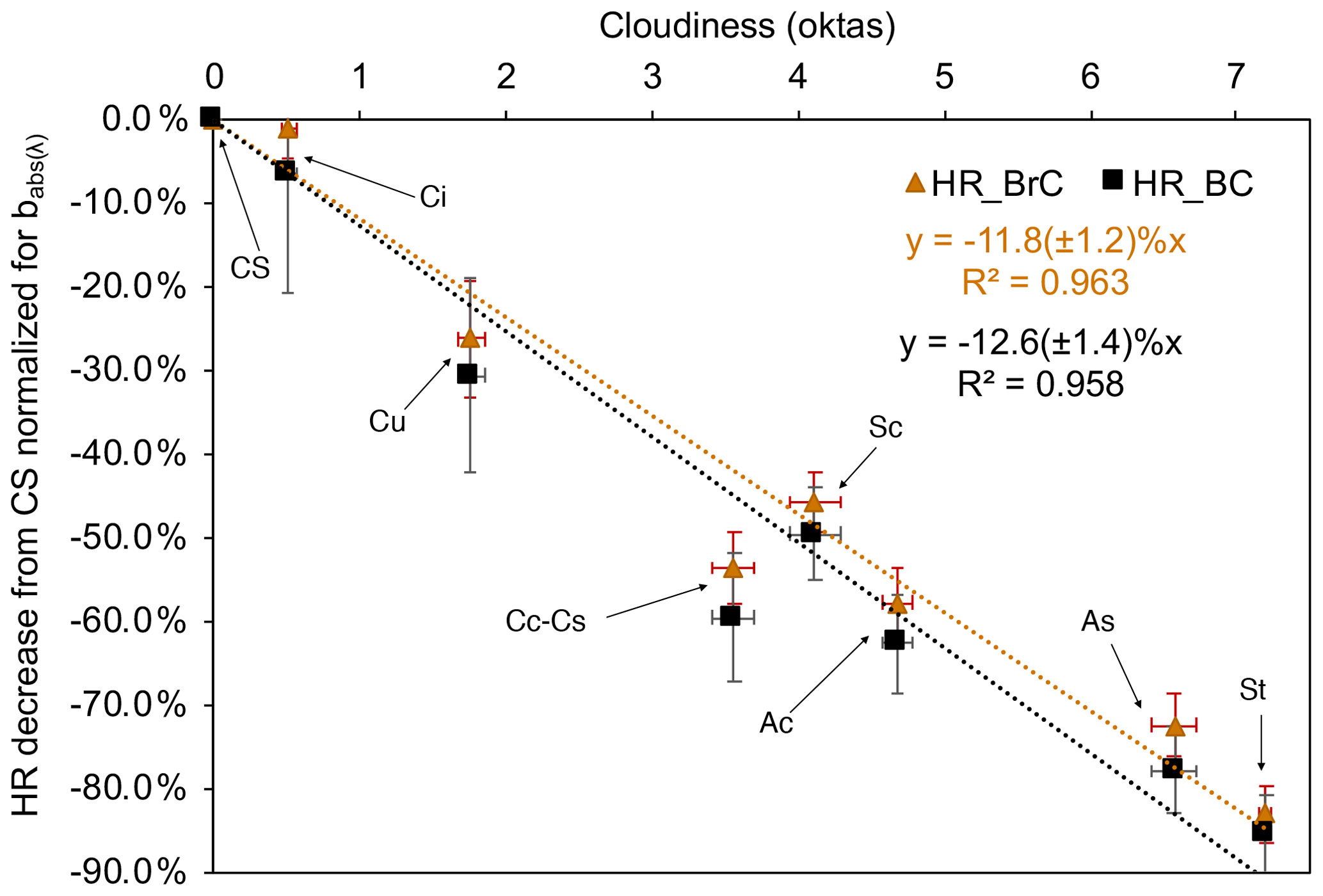
Figure 16Percentage decrease of the HRBC and HRBrC with respect to clear-sky conditions as a function of cloudiness (oktas) averaged for each cloud type.
Here we focus on the fact that the magnitude of babs(λ) of BC and BrC changed differently with cloudiness. Thus, in order to decouple the variability of the HR induced by the varying incoming irradiance from that due to changes in babs(λ), both the HRBC and HRBrC were normalized to the dimensionless integral of babs(λ) over the whole aethalometer spectrum. In this way, the magnitude of babs(λ) is accounted for along the whole spectrum, avoiding the choice of an arbitrary wavelength as a reference for the normalization. Similarly to Sect. 3.2.2 for the total of the LAA HR, the variability of the normalized HRBC and HRBrC was investigated with respect to cloudiness and cloud type; in this respect, both the HRBC and HRBrC were normalized to the dimensionless integral of babs(λ) for each cloud type. Figure 16a shows the decrease of the normalized HRBC and HRBrC as a function of average cloudiness for each cloud type. We found a strong linear relationship between the decrease of both the normalized HRBC and HRBrC (relative to CS conditions) and the mean cloudiness (in oktas) for each cloud type. Focusing on the cloud type, Ci clouds were found to produce a statistically negligible impact on cloudiness (0.50 ± 0.05 oktas), decreasing the HRBC and HRBrC by ∼ 1 %–6 %, respectively. Cu clouds (1.76 ± 0.09 oktas) decreased the HRBC and HRBrC by −31 ± 12 % and −26 ± 7 %, respectively. Cc–Cc clouds featured 3.56 ± 0.14 oktas and were responsible for a −60 ± 8 % and −54 ± 4 % decrease of the HRBC and HRBrC. Their impact was comparable to that of Ac (4.11 ± 0.18 oktas): −60 ± 6 % and −46 ± 4 % decrease of the HRBC and HRBrC. Sc clouds (4.68 ± 0.10 oktas) had a higher impact, decreasing the HRBC and HRBrC of −63 ± 6 % and −58 ± 4 %. The highest impact was given by As (6.57 ± 0.15 oktas; −78 ± 5 % and −73 ± 4 % of the HRBC and HRBrC) and by St (7.19 ± 0.04 oktas), suppressing the HRBC and HRBrC by −85 ± 5 % and −83 ± 3 %, respectively.
Overall, the derived linear regressions indicate a decrease of ∼ 12 % per okta for both the HRBC and HRBrC (with high R2 of 0.958 and 0.963, respectively). In detail, the respective decreases of the HRBC and HRBrC were −11.8 ± 1.2 % and −12.6 ± 1.4 % per okta, with these values not being statistically different. We show that, while BC and BrC have different optical properties and wavelength dependence of absorption, their HR normalized to absorption changed without any statistical difference as a function of cloudiness and cloud type. This simplifies the models and reduces the number of details needed to be considered: once the HRBC and HRBrC are determined in clear-sky conditions, their dependence on the cloudiness can be determined from the simple reduction of the HR normalized to the absorption coefficient (about 12 % for both species, once dominant cloud type is known).
However, it noteworthy that the normalized HRBrC values in Fig. 16 were always greater than or equal to the corresponding ones of BC (even if 95 % confidence interval bands overlapped). A possible explanation can be the synergic effect between the different spectral absorption of BC and BrC and the influence of clouds on the energy of the impinging radiation; this is detailed in the Supplement (“The role of average photon energy on the HR of BC and BrC”). This feature needs further investigation in other seasons and elsewhere in the world where the prevailing cloud types and the light absorption by BrC might be different.
The heating rates (HRs) associated with the two major LAA species, i.e. black carbon (BC) and brown carbon (BrC) (HRBC and HRBrC), were experimentally determined based on radiation and aerosol measurements (at high time resolution) in the Po Valley. We determined the impact of cloud–aerosol–radiation interactions on the atmospheric heating by examining the total HR in different sky conditions. Results showed a constant decrease of the LAA HR with increasing cloudiness of the atmosphere (∼ 12 %). Our real-atmosphere, all-sky, measurement-based results suggest that using a simplified assumption of clear-sky conditions in radiative-transfer calculations might overestimate the HR by over 400 %. The effect of different cloud types on the HR was also investigated. While cirrus clouds were characterized by a modest impact, cumulus, cirrocumulus–cirrostratus and altocumulus suppressed the HR of both BC and BrC by a factor of ∼ 2. Stratocumulus, altostratus and stratus clouds suppressed the HRBC and HRBrC up to 80 %. The cloudiness also changed the diurnal pattern of the HR with possible feedbacks on planetary boundary layer dynamics and/or regional circulation systems.
The total HR, HRBC and HRBrC are affected by both cloudiness and cloud type so that inaccurate HRBC and HRBrC estimations can be derived from simulations if presence of clouds is ignored and cloud type is not taken into account. Most importantly, the coupling between the cloud impact on the solar radiation spectrum (and its direct, diffuse and reflected components) and the spectral-absorption properties of BC and BrC showed that the absolute HRBC and HRBrC vary differently with cloudiness (especially the diffuse component) but feature a very similar normalized (to the absorption coefficient) dependence on the cloudiness. This simplifies the models and reduces the number of details that need to be considered: once the HRBC and HRBrC are determined in clear-sky conditions, their dependence on the cloudiness can be determined from the simple reduction of the HR normalized to the absorption coefficient (about 12 % per okta for both species). These data acquire importance when discussed in the context of the counterintuitive semi-direct effect proposed by Perlwitz and Miller (2010): the atmospheric heating induced by tropospheric absorbing aerosol could lead to a cloud cover increase stressing the need for a proper determination and simulation of sky conditions during radiative-transfer calculations.
| Aerosol acronyms | |
| AAE | Absorption Ångström exponent |
| AAEBC | Absorption Ångström exponent of black carbon |
| AAEBrC | Absorption Ångström exponent of brown carbon |
| babs(λ) | Wavelength-dependent aerosol absorption coefficient (Mm−1) |
| BC | Black carbon |
| BrC | Brown carbon |
| eBC | Equivalent black carbon concentration (µg m−3) |
| LAA | Light-absorbing aerosol |
| HR | Heating rate (K d−1) |
| HRBC | Heating rate of black carbon (K d−1) |
| HRBrC | Heating rate of brown carbon (K d−1) |
| Cloud and sky acronyms | |
| As | Altostratus |
| Ac | Altocumulus |
| Ci | Cirrus |
| Cc–Cs | Cirrocumulus–cirrostratus |
| Cu | Cumulus |
| CS | Clear-sky conditions |
| St | Stratus |
| Sc | Stratocumulus |
| CBH | Cloud base height (km) |
| N | Classes of sky conditions in oktas (from 0 for clear-sky conditions to 8 for completely overcast) |
| Rt | Ratio (R) between observed global irradiance (Fglo) and the modelled clear-sky irradiance (Fglo_CS) |
| SDt | SD of the measured Fglo in 20 min time intervals (W m−2) |
| Sft | Scaling factor Sft (Duchon and O'Malley, 1999) |
| Other symbols and acronyms | |
| φ | Azimuth angle (rad) |
| Φλ | Photon flux density at wavelength λ () |
| λ | Wavelength (nm) |
| ρ | Air density (kg m−3) |
| θ | Zenith angle (rad) |
| θz | Solar zenith angle (rad) |
| a | Empirical coefficient from Ehnberg and Bollen (2005); Table S1 |
| a0 | Empirical coefficient from Ehnberg and Bollen (2005); Table S1 |
| a1 | Empirical coefficient from Ehnberg and Bollen (2005); Table S1 |
| a3 | Empirical coefficient from Ehnberg and Bollen (2005); Table S1 |
| AF(λ) | Actinic flux for wavelength λ () |
| APE | Average photon energy (eV) |
| APEdif | Average photon energy for diffuse radiation (eV) |
| APEdir | Average photon energy for direct radiation (eV) |
| APEref | Average photon energy for reflected radiation (eV) |
| c | Speed of light (m s−1) |
| Cp | Isobaric specific heat of dry air (1005 ) |
| dif | Diffuse |
| dir | Direct |
| Fglo | Global broadband irradiance; (W m−2) |
| Fdif | Diffuse broadband irradiance (W m−2) |
| Fdir | Direct broadband irradiance (W m−2) |
| Fref | Reflected broadband irradiance (W m−2) |
| Fdir,dif,ref(λ) | Spectral irradiance as a function of λ () |
| h | Plank constant (J s) |
| ref | Reflected |
| L | Empirical coefficient from Ehnberg and Bollen (2005); Table S1 |
| q | Electron charge (C) |
| Radiance at wavelength λ from zenith and azimuth angles θ and φ () | |
The validation was conducted in two subsequent steps. In the first step the automatized cloud classification (based on Duchon and O'Malley, 1999; including lidar cloud base height) was compared to the visual cloud classification based on sky images collected during 1 month of a field campaign.
The second validation step involved the recently published method discussed by Ylivinkka et al. (2020), which is based on the same methodological approach used in this study: the application of the Duchon and O'Malley (1999) classification improved by the knowledge of the CBH. Thus, the aim of the second step was to determine the degree of consistency between the two approaches that were developed simultaneously and independently in two different regions of the globe.
Both the two validations were evaluated by means of a confusion matrix, a special kind of contingency table, with two dimensions and identical sets of “classes” in both of them. From the confusion matrix the balanced accuracy was computed as follows:
where the Sensitivity describes the true positive rate (the number of correct positive predictions divided by the total number of positives) and the Specificity describes the true negative rate (the number of correct negative predictions divided by the total number of negatives). The balanced accuracy is especially useful when the investigated classes are imbalanced; i.e. one of the classes appears a lot more often than the other, a condition useful for cloud classification (García et al., 2009).
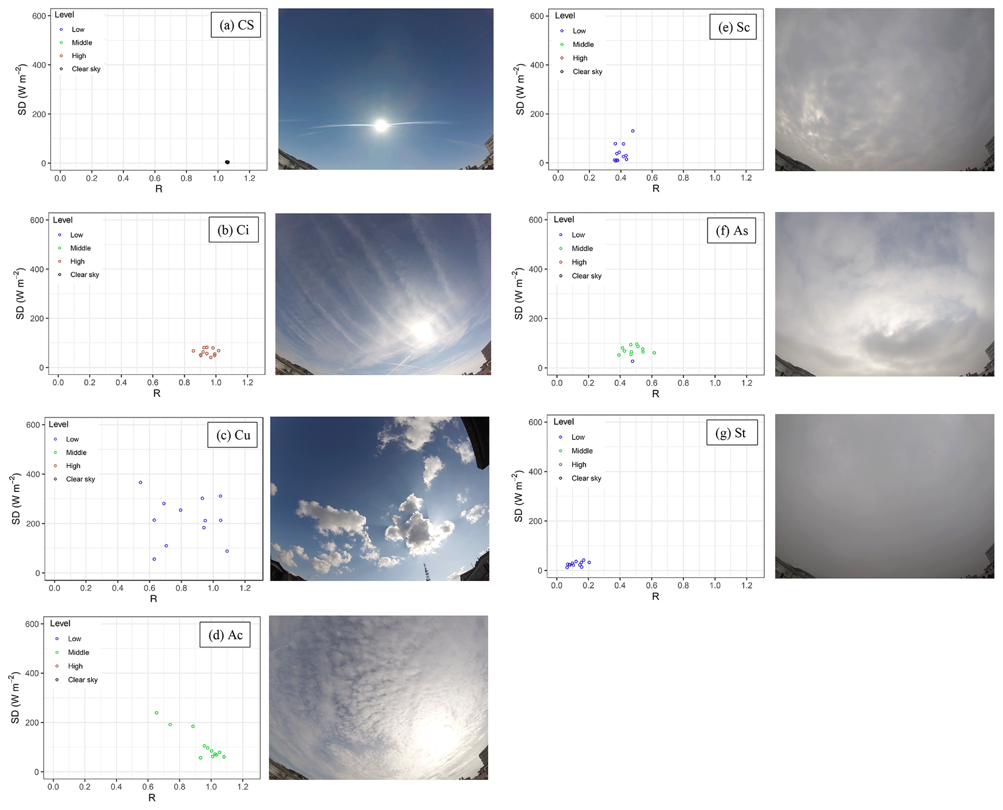
Figure B1SD–R diagram (a–g) and the corresponding sky images for the February–March 2017 field campaign: (a) CS conditions, (b) Ci clouds, (c) Cu clouds, (d) Ac clouds, (e) Sc clouds, (f) As clouds and (g) St clouds.
B1 Visual cloud classification
Sky images were collected during 1 month (13 February–9 March 2017) using a sky view camera (GoPro Hero4 Session installed on the U9 roof), characterized by a field of view of 95∘ × 123∘; the camera was oriented south (each day manually) with the same declination of the shadow band applied to the DPA154 global radiometer (for diffuse broadband irradiance measurements, Sect. 2.1.2); sky images were taken with 1 min time resolution. Visual classification of sky images, based on the principles of cloud classification published in the International Cloud Atlas (WMO). Figure B1 reports an example of the SD–R diagram (Sect. 2.3.2) with the CBH for each sky or cloud condition with the corresponding image.
To test the performance, 869 sky images were analysed, and the cloud type was determined through visual inspection. From the visual classification and the automatized one (Table 1) the following confusion matrix (Table B1) was created. The highest balanced accuracy was found for St data (95 %), while the lowest (50 %) was found for mixed cloud types (Cc–Cs) whose absolute number of cases, however, was ∼ 0.6 % of the total, probably biassing the obtained accuracy; the same happened for Cu and Ac. Overall, five of eight classes were above 68 % of balanced accuracy, while the overall balanced accuracy was 80 %, underlying the reliability of the classification algorithm, allowing for studying the impact of clouds on the LAA HR with a sufficient grade of certainty.
Table B1Confusion matrix and balanced accuracy for each cloud type classified visually and following the algorithm reported in Table 1 within the present work.
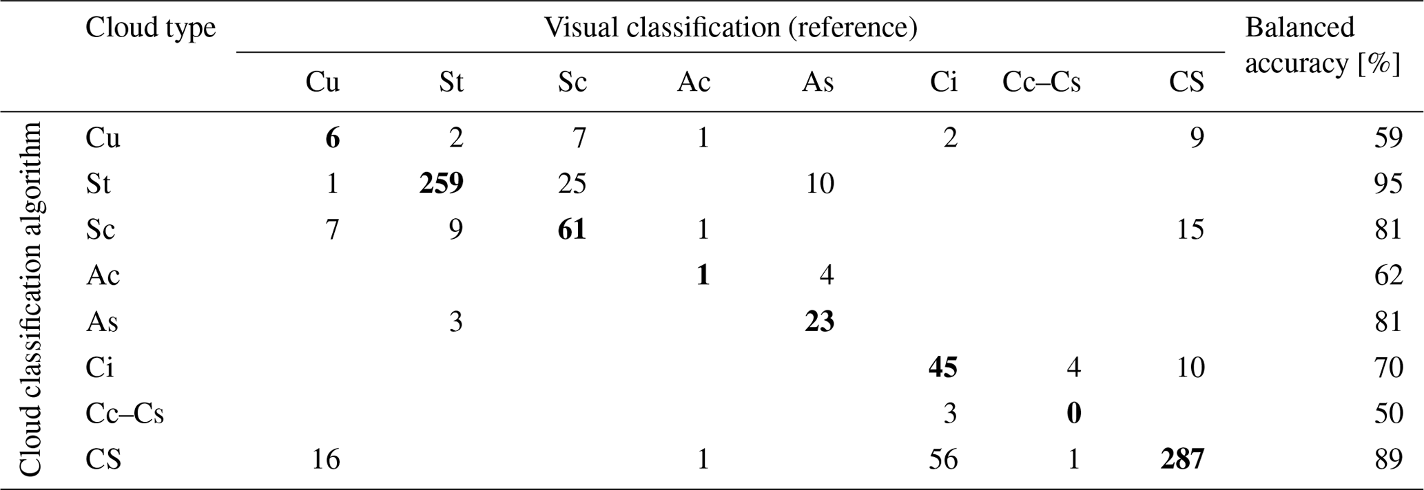
Table B2Final criteria adopted for cloud classification in Ylivinkka et al. (2020). Ns here represents nimbostratus, while GRE stands for global radiation enhancement.
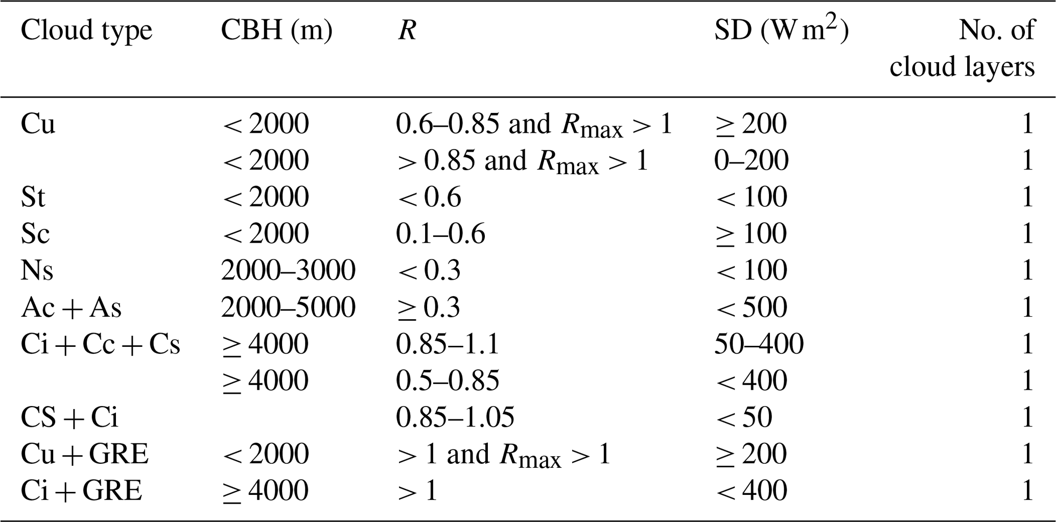
Table B3Cloud class homogenization adopted for comparison purposes (merged cloud type) between the present study's cloud classification and the one reported in Ylivinkka et al. (2020).
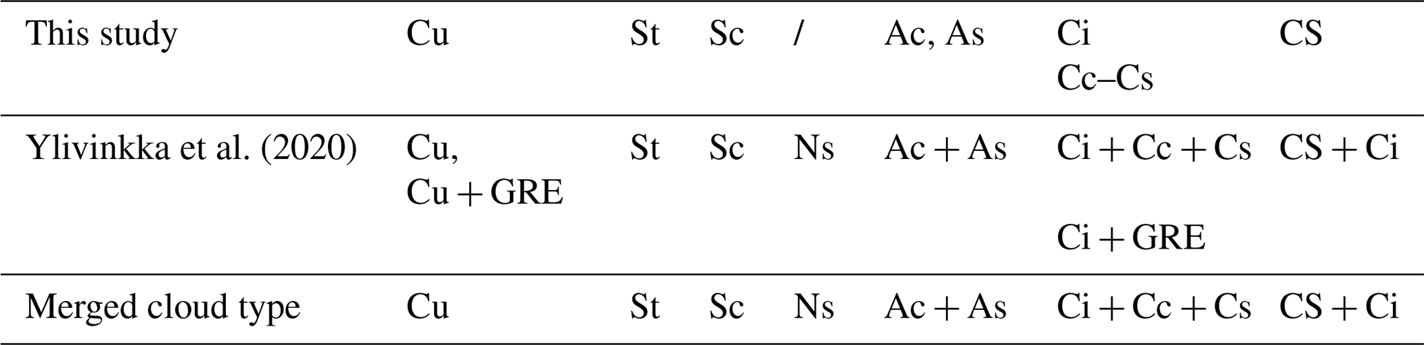
Table B4Confusion matrix and balanced accuracy for each cloud type classified using the algorithm reported in the present study and the one reported in Ylivinkka et al. (2020).

B2 Intercomparison with Ylivinkka et al. (2020)
The second validation step involved the recently published method discussed by Ylivinkka et al. (2020), which is based on the same logical approach followed in our work: the application of the Duchon and O'Malley (1999) classification improved by the knowledge of the CBH. For this purpose, the classification scheme of Ylivinkka et al. (2020) is resumed in Table B2 following the nomenclature used in the present work. It is necessary to underline that the cloud classes determined in the work of Ylivinkka et al. (2020) differ from those reported in the present work. Particularly, while both approaches enabled the Cu, St and Sc classification, some of the cloud classes were merged in the Ylivinkka et al. (2020) study: CS and Ci (CS + Ci); Ac and As (Ac + As); and a mixed situation composed by Ci, Cc and Cs (Ci + Cc + Cs). In addition they introduced the classes Cu + GRE and Ci + GRE to account for global radiation enhancement (GRE) due to this cloud types; a possible explanation for such a difference with respect to present work could be hidden in the different latitude at which the two algorithms were developed, which is a parameter able to affect the solar zenith angle and the sun light interaction with clouds. A detailed investigation of this difference is beyond the aim of the present work. However, it is necessary to account for the classification differences in order to properly merge cloud classes with similar features to finally perform a comparison between the two methods. The cloud class homogenization is summarized in Table B3, while the final intercomparison is reported in Table B4. The confusion matrix (Table B4) revealed a global balanced accuracy of 90 %, making the two methods comparable, despite the aforementioned differences. The highest accuracy (100 %) was obtained for CS, followed by Ac + As (99 %); Cu, St and Sc reached values of 94 %, 93 % and 86 %, respectively. The lowest performance was reached for Ns, whose presence cannot be detected in the present study, generating a false positive signal in the Ac + As class; however, due to the very low number of Ns cases (1.8 %), its impact on the cloud classification can be neglected. Overall, even the second validation step pointed out the reliability of the results obtained in the present work.
Data are available upon request.
The supplement related to this article is available online at: https://doi.org/10.5194/acp-21-4869-2021-supplement.
LF, EB, GM, MR and AG conceptualized the project. LF, AG, SC, NK, FB, LDL and GPG designed the methodology. LF, AG, SC, FB, GM and MR performed the data investigation. EB and MR procured resources. LF prepared the original draft of the paper. LF, AG, GM and FB reviewed and edited the paper. GM, MR, FB and EB supervised the project.
The authors declare that they have no conflict of interest. The funders had no role in the design of the study; in the collection, analyses or interpretation of data; in the writing of the paper; and in the decision to publish the results.
This paper is an output of the GEMMA research centre in the framework of the MIUR project “Dipartimenti di Eccellenza 2018-2022”. The work was in part funded by the Slovenian Research Agency programme “Remote sensing of atmospheric properties” (no. P1-0385). The authors want to acknowledge the COST action COLOSSAL CA16109, Aerosol d.o.o and LSI Lastem for their cooperation during the campaign.
This research has been supported by MIUR (grant “Dipartimenti di Eccellenza 2018–2022”) and by the Slovenian Research Agency programme “Remote sensing of atmospheric properties” (grant no. P1-0385).
This paper was edited by Urs Baltensperger and reviewed by two anonymous referees.
Ahrens, C. D.: Meteorology Today – An Introduction to Weather, Climate and Environment, ninth edn., Brooks/Cole, Pacific Grove, California, 2009.
Andreae, M. and Ramanathan, V.: Climate's Dark Forcings, Science, 340, 280–281, 2013.
Arnott, W. P., Hamasha, K., Moosmüller, H., Sheridan, P. J., and Ogren, J. A.: Towards Aerosol Light-Absorption Measurements with a 7-Wavelength Aethalometer: Evaluation with a Photoacoustic Instrument and 3-Wavelength Nephelometer, Aerosol Sci. Tech., 39, 17–29, https://doi.org/10.1080/027868290901972, 2005.
Barnaba, F. and Gobbi, G. P.: Aerosol seasonal variability over the Mediterranean region and relative impact of maritime, continental and Saharan dust particles over the basin from MODIS data in the year 2001, Atmos. Chem. Phys., 4, 2367–2391, https://doi.org/10.5194/acp-4-2367-2004, 2004.
Barnaba, F., Putaud, J. P., Gruening, C., Dell'Acqua, A., and Dos Santos, S.: Annual cycle in co-located in situ, total-column, and height- resolved aerosol observations in the Po Valley (Italy): Implications for ground-level particulate matter mass concentration estimation from remote sensing, J. Geophys. Res., 115, D19209, https://doi.org/10.1029/2009JD013002, 2010.
Bartoszek, K., Matuszko, D., and Soroka, J.: Relationships between cloudiness, aerosol optical thickness, and sunshine duration in Poland, Atmos. Res., 245, 105097, https://doi.org/10.1016/j.atmosres.2020.105097, 2020.
Boers, R., de Haij, M. J., Wauben, W., Baltink, H. K., van Ulft, L. H., Savenije, M., and Long, C. N.: Optimized fractional cloudiness determination from five ground-based remote sensing techniques, J. Geophys. Res., 115, D24116. https://doi.org/10.1029/2010JD014661, 2010.
Bond, T. C. and Bergstrom, R. W.: Light Absorption by Carbonaceous Particles: An Investigative Review, Aerosol Sci. Tech., 40, 27–67, https://doi.org/10.1080/02786820500421521, 2006.
Bond, T. C., Doherty, S. J., Fahey, D. W., Forster, P. M., Berntsen, T., Deangelo, B. J., Flanner, M. G., Ghan, S., Kärcher, B., Koch, D., Kinne, S., Kondo, Y., and Quinn, P. K.: Bounding the role of black carbon in the climate system: A scientific assessment, J. Geophys. Res., 118, 1–173, https://doi.org/10.1002/jgrd.50171, 2013.
Calbó, J. and Sabburg, J.: Feature extraction from Whole-sky ground-based images for cloud-type recognition, J. Atmos. Ocean. Tech., 25, 3–14, https://doi.org/10.1175/2007JTECHA959.1, 2008.
Calbó, J., González, J. A., and Pagès, D.: A method for sky-condition classification from ground-based solar radiation measurements, J. Appl. Meteorol., 40, 2193–2199, 2001.
Calbó, J., Pagès, D., and González, J.-A.: Empirical studies of cloud effects on UV radiation: A review, Rev. Geophys., 43, RG2002, https://doi.org/10.1029/2004RG000155, 2005.
Campbell, J. R., Lolli, S., Lewis, J. R., Gu, Y., and Welton, E. J.: Daytime Cirrus Cloud Top-of-the-Atmosphere Radiative Forcing Properties at a Midlatitude Site and Their Global Consequences, J. Appl. Meteorol. Clim., 55, 1667–1679, 2016.
Carbone, C., Decesari, S., Mircea, M., Giulianelli, L., Finessi, E., Rinaldi, M., Fuzzi, S., Marinoni, A., Duchi, R., Perrino, C., Sargolini, T., Vardè, M., Sprovieri, F., Gobbi, G. P., Angelini, F., and Facchini, M. C.: Size-resolved aerosol chemical composition over the Italian Peninsula during typical summer and winter conditions, Atmos. Environ., 44, 5269–5278, https://doi.org/10.1016/j.atmosenv.2010.08.008, 2010.
Chung, C. E., Ramanathan, V., and Decremer, D.: Observationally constrained estimates of carbonaceous aerosol radiative forcing, P. Natl. Acad. Sci. USA, 109, 11624–11629, 2012.
Cogliati, S., Rossini, M., Julitta, T., Meroni, M., Schickling, A., Burkart, A., Pinto, F., Rascher, U., and Colombo, R.: Continuous and long-term measurements of reflectance and sun-induced chlorophyll fluorescence by using novel automated field spectroscopy systems, Remote Sens. Environ., 164, 270–281, https://doi.org/10.1016/j.rse.2015.03.027, 2015.
Collaud Coen, M., Weingartner, E., Apituley, A., Ceburnis, D., Fierz-Schmidhauser, R., Flentje, H., Henzing, J. S., Jennings, S. G., Moerman, M., Petzold, A., Schmid, O., and Baltensperger, U.: Minimizing light absorption measurement artifacts of the Aethalometer: evaluation of five correction algorithms, Atmos. Meas. Tech., 3, 457–474, https://doi.org/10.5194/amt-3-457-2010, 2010.
Costa-Surós, M., Calbó, J., González, J. A., and Martin-Vide, J.: Behavior of cloud base height from ceilometer measurements, Atmos. Res., 127, 64–76, https://doi.org/10.1016/j.atmosres.2013.02.005, 2013.
Costabile, F., Barnaba, F., Angelini, F., and Gobbi, G. P.: Identification of key aerosol populations through their size and composition resolved spectral scattering and absorption, Atmos. Chem. Phys., 13, 2455–2470, https://doi.org/10.5194/acp-13-2455-2013, 2013.
Cotton, W. R., Bryan, G. H., and Van de Heever, S. C.: Storm and cloud dynamics, second edn., in: International Geophysics Series, vol. 99, Elsevier-Academic Press, New York, London, 826 pp., 2011.
Croke, M. S., Cess, R. D., and Hameed, S.: Regional cloud cover change associated with global climate change: Case studies for three regions of the United States, J. Climate, 12, 2128–2134, 1999.
Curci, G., Ferrero, L., Tuccella, P., Barnaba, F., Angelini, F., Bolzacchini, E., Carbone, C., Denier van der Gon, H. A. C., Facchini, M. C., Gobbi, G. P., Kuenen, J. P. P., Landi, T. C., Perrino, C., Perrone, M. G., Sangiorgi, G., and Stocchi, P.: How much is particulate matter near the ground influenced by upper-level processes within and above the PBL? A summertime case study in Milan (Italy) evidences the distinctive role of nitrate, Atmos. Chem. Phys., 15, 2629–2649, https://doi.org/10.5194/acp-15-2629-2015, 2015.
D'Angelo, L., Rovelli, G., Casati, M., Sangiorgi, G., Perrone, M. G., Bolzacchini, E., and Ferrero, L.: Seasonal behavior of PM2.5 deliquescence, crystallization, and hygroscopic growth in the Po Valley (Milan): Implications for remote sensing applications, Atmos. Res., 176–177, 87–95, https://doi.org/10.1016/j.atmosres.2016.02.011, 2016.
Di Nicolantonio, W., Cacciari, A., Bolzacchini, E., Ferrero, L., Volta, M., and Pisoni, E.: MODIS aerosol optical properties over north Italy for estimating surface-level PM2.5, in: Proc. Envisat Symposium 2007, Montreux, Switzerland, 23–27 April 2007 (ESA SP-636, July 2007), available at: http://envisat.esa.int/ envisatsymposium/proceedings/posters/3P5/464392wd.pdf (last access: 24 March 2021), 2007.
Di Nicolantonio, W., Cacciari, A., Petritoli, A., Carnevale, C., Pisoni, E., Volta, M. L., Stocchi, P., Curci, G., Bolzacchini, E., Ferrero, L., Ananasso, C., and Tomasi, C.: MODIS and OMI satellite observations supporting air quality monitoring, Radiat. Prot. Dosim., 137, 280–287, 2009.
Diémoz, H., Barnaba, F., Magri, T., Pession, G., Dionisi, D., Pittavino, S., Tombolato, I. K. F., Campanelli, M., Della Ceca, L. S., Hervo, M., Di Liberto, L., Ferrero, L., and Gobbi, G. P.: Transport of Po Valley aerosol pollution to the northwestern Alps – Part 1: Phenomenology, Atmos. Chem. Phys., 19, 3065–3095, https://doi.org/10.5194/acp-19-3065-2019, 2019a.
Diémoz, H., Gobbi, G. P., Magri, T., Pession, G., Pittavino, S., Tombolato, I. K. F., Campanelli, M., and Barnaba, F.: Transport of Po Valley aerosol pollution to the northwestern Alps – Part 2: Long-term impact on air quality, Atmos. Chem. Phys., 19, 10129–10160, https://doi.org/10.5194/acp-19-10129-2019, 2019b.
Dionisi, D., Barnaba, F., Diémoz, H., Di Liberto, L., and Gobbi, G. P.: A multiwavelength numerical model in support of quantitative retrievals of aerosol properties from automated lidar ceilometers and test applications for AOT and PM10 estimation, Atmos. Meas. Tech., 11, 6013–6042, https://doi.org/10.5194/amt-11-6013-2018, 2018.
Drinovec, L., Močnik, G., Zotter, P., Prévôt, A. S. H., Ruckstuhl, C., Coz, E., Rupakheti, M., Sciare, J., Müller, T., Wiedensohler, A., and Hansen, A. D. A.: The “dual-spot” Aethalometer: an improved measurement of aerosol black carbon with real-time loading compensation, Atmos. Meas. Tech., 8, 1965–1979, https://doi.org/10.5194/amt-8-1965-2015, 2015.
Duchon, C. E. and O'Malley, M.: Estimating Cloud Type from Pyranometer Observations, J. Appl. Meteorol., 38, 132–141, 1999.
Ehnberg, J. S. G. and Bollen, M. H. J.: Simulation of global solar radiation based on cloud observations, Sol. Energy, 78, 157–162, https://doi.org/10.1016/j.solener.2004.08.016, 2005.
Eleftheriadis, K., Vratolis, S., and Nyeki, S.: Aerosol black carbon in the European Arctic: Measurements at Zeppelin station, Ny-Ålesund, Svalbard from 1998–2007, Geophys. Res. Lett., 36, L02809, https://doi.org/10.1029/2008GL035741, 2009.
Feister, U., Cabrol, N., and Häder, D.: UV Irradiance Enhancements by Scattering of Solar Radiation from Clouds, Atmosphere, 6, 1211–1228, https://doi.org/10.3390/atmos6081211, 2015.
Ferrero, L., Perrone, M. G., Petraccone, S., Sangiorgi, G., Ferrini, B. S., Lo Porto, C., Lazzati, Z., Cocchi, D., Bruno, F., Greco, F., Riccio, A., and Bolzacchini, E.: Vertically-resolved particle size distribution within and above the mixing layer over the Milan metropolitan area, Atmos. Chem. Phys., 10, 3915–3932, https://doi.org/10.5194/acp-10-3915-2010, 2010.
Ferrero, L., Riccio, A., Perrone, M. G., Sangiorgi, G., Ferrini, B. S., and Bolzacchini, E.: Mixing height determination by tethered balloon-based particle soundings and modeling simulations, Atmos. Res, 102, 145–156, https://doi.org/10.1016/j.atmosres.2011.06.016, 2011a.
Ferrero, L., Mocnik, G., Ferrini, B. S., Perrone, M. G., Sangiorgi, G., and Bolzacchini, E.: Vertical profiles of aerosol absorption coefficient from micro-Aethalometer data and Mie calculation over Milan, Sci. Total Environ., 409, 2824–37, https://doi.org/10.1016/j.scitotenv.2011.04.022, 2011b.
Ferrero, L., Cappelletti, D., Moroni, B., Sangiorgi, G., Perrone, M. G., Crocchianti, S., and Bolzacchini, E.: Wintertime aerosol dynamics and chemical composition across the mixing layer over basin valleys, Atmos. Environ., 56, 143–153, https://doi.org/10.1016/j.atmosenv.2012.03.071, 2012.
Ferrero, L., Sangiorgi, G., Ferrini, B. S., Perrone, M. G., Moscatelli, M., D'Angelo, L., Rovelli, G., Ariatta, A., Truccolo, R., and Bolzacchini, E.: Aerosol corrosion prevention and energy-saving strategies in the design of green data centers, Environ. Sci. Technol., 47, 3856–64, https://doi.org/10.1021/es304790f, 2013.
Ferrero, L., Castelli, M., Ferrini, B. S., Moscatelli, M., Perrone, M. G., Sangiorgi, G., D'Angelo, L., Rovelli, G., Moroni, B., Scardazza, F., Močnik, G., Bolzacchini, E., Petitta, M., and Cappelletti, D.: Impact of black carbon aerosol over Italian basin valleys: high-resolution measurements along vertical profiles, radiative forcing and heating rate, Atmos. Chem. Phys., 14, 9641–9664, https://doi.org/10.5194/acp-14-9641-2014, 2014.
Ferrero, L., D'Angelo, L., Rovelli, G., Sangiorgi, G., Perrone, M. G., Moscatelli, M., Casati, M., Rozzoni, V., and Bolzacchini, E.: Determination of aerosol deliquescence and crystallization relative humidity for energy saving in free-cooled data centers, Int. J. Environ. Sci. Te., 12, 2777–2790, https://doi.org/10.1007/s13762-014-0680-2, 2015.
Ferrero, L., Cappelletti, D., Busetto, M., Mazzola, M., Lupi, A., Lanconelli, C., Becagli, S., Traversi, R., Caiazzo, L., Giardi, F., Moroni, B., Crocchianti, S., Fierz, M., Močnik, G., Sangiorgi, G., Perrone, M. G., Maturilli, M., Vitale, V., Udisti, R., and Bolzacchini, E.: Vertical profiles of aerosol and black carbon in the Arctic: a seasonal phenomenology along 2 years (2011–2012) of field campaigns, Atmos. Chem. Phys., 16, 12601–12629, https://doi.org/10.5194/acp-16-12601-2016, 2016.
Ferrero, L., Močnik, G., Cogliati, S., Gregorič A., Colombo, R., and Bolzacchini, E.: Heating Rate of Light Absorbing Aerosols: Time-Resolved Measurements, the Role of Clouds, and Source Identification, Environ. Sci. Techol., 52, 3546–3555, https://doi.org/10.1021/acs.est.7b04320, 2018.
Ferrero, L., Ritter, C., Cappelletti, D., Moroni, B., Močnik, G., Mazzola, M., Lupi, A., Becagli, S., Traversi, R., Cataldi, M., Neuber, R., Vitale, V., and Bolzacchini, E: Aerosol optical properties in the Arctic: the role of aerosol chemistry and dust composition in a closure experiment between Lidar and tethered balloon vertical profiles, Sci. Total Environ., 686, 452–467, https://doi.org/10.1016/j.scitotenv.2019.05.399, 2019.
Galli, C., Nardino, M., Levizzani, V., Rizzi, R., and Georgiadis, T.: Radiative energy partition and cloud radiative forcing at a Po valley site, Atmos. Res., 72, 329–351, https://doi.org/10.1016/j.atmosres.2004.03.022, 2004.
Gao, R. S., Hall, S. R., Swartz, W. H., Schwarz, J. P., Spackman, J. R., Watts, L. A., Fahey, D. W., Aikin, K. C., Shetter, R. E., and Bui, T. P.: Calculations of solar shortwave heating rates due to black carbon and ozone absorption using in situ measurements, J. Geophys. Res.-Atmos., 113, 14–19, https://doi.org/10.1029/2007JD009358, 2008.
García, V., Mollineda, R. A., and Sánchez, J. S.: Index of Balanced Accuracy: A Performance Measure for Skewed Class Distributions, in: Pattern Recognition and Image Analysis. IbPRIA 2009, Lecture Notes in Computer Science, vol 5524, edited by: Araujo, H., Mendonça, A. M., Pinho, A. J., and Torres, M. I., Springer, Berlin, Heidelberg, https://doi.org/10.1007/978-3-642-02172-5_57, 2009.
Harrison, R. G., Chalmers, N., and Hogan, R. J.: Retrospective cloud determinations from surface solar radiation measurements, Atmos. Res., 90, 54–62, https://doi.org/10.1016/j.atmosres.2008.04.001, 2008.
Hirsch, E., Agassi, E., and Koren, I.: A novel technique for extracting clouds base height using ground based imaging, Atmos. Meas. Tech., 4, 117–130, https://doi.org/10.5194/amt-4-117-2011, 2011.
Huertas-Tato, J., Rodríguez-Benítez, F. J., Arbizu-Barrena, C., Aler-Mur, R., Galvan-Leon, I., and Pozo-Vázquez, D.: Automatic Cloud-Type Classification Based On the Combined Use of a Sky Camera and a Ceilometer, J. Geophys. Res.-Atmos., 122, 11,045–11,061, https://doi.org/10.1002/2017JD027131, 2017.
IPCC: Climate Change 2013: The Physical Science Basis, Cambridge University Press, Cambridge, UK and New York, USA, 2013.
Jacobson, M. Z.: Control of fossil-fuel particulate black carbon and organic matter, possibly the most effective method of slowing global warming, J. Geophys. Res., 107, 4410, https://doi.org/10.1029/2001JD001376, 2002.
Junker, C., Jennings, S. G., and Cachier, H.: Aerosol light absorption in the North Atlantic: trends and seasonal characteristics during the period 1989 to 2003, Atmos. Chem. Phys., 6, 1913–1925, https://doi.org/10.5194/acp-6-1913-2006, 2006.
Kaufman, Y. J., Tanré, D., and Boucher, O.: A satellite view of aerosols in the climate system, Nature, 419, 215–223, 2002.
Kirchstetter, T. W., Novakov, T., and Hobbs, P. V.: Evidence that the spectral dependence of light absorption by aerosols is affected by organic carbon, J. Geophys. Res.-Atmos., 109, 1–12, https://doi.org/10.1029/2004JD004999, 2004.
Koch, D. and Del Genio, A. D.: Black carbon semi-direct effects on cloud cover: review and synthesis, Atmos. Chem. Phys., 10, 7685–7696, https://doi.org/10.5194/acp-10-7685-2010, 2010.
Koch, D., Schulz, M., Kinne, S., McNaughton, C., Spackman, J. R., Balkanski, Y., Bauer, S., Berntsen, T., Bond, T. C., Boucher, O., Chin, M., Clarke, A., De Luca, N., Dentener, F., Diehl, T., Dubovik, O., Easter, R., Fahey, D. W., Feichter, J., Fillmore, D., Freitag, S., Ghan, S., Ginoux, P., Gong, S., Horowitz, L., Iversen, T., Kirkevåg, A., Klimont, Z., Kondo, Y., Krol, M., Liu, X., Miller, R., Montanaro, V., Moteki, N., Myhre, G., Penner, J. E., Perlwitz, J., Pitari, G., Reddy, S., Sahu, L., Sakamoto, H., Schuster, G., Schwarz, J. P., Seland, Ø., Stier, P., Takegawa, N., Takemura, T., Textor, C., van Aardenne, J. A., and Zhao, Y.: Evaluation of black carbon estimations in global aerosol models, Atmos. Chem. Phys., 9, 9001–9026, https://doi.org/10.5194/acp-9-9001-2009, 2009.
Koren, I., Kaufman, Y. J., Remer, L. A., and Martins, J. V.: Measurments of the effect of amazon smoke on inhibition of cloud formation, Science, 303, 1342–1345, 2004.
Koren, I., Martins, J. V., Remer, L. A., and Afargan, H.: Smoke invigoration versus inhibition of clouds over the amazon, Science, 321, 946–949, 2008.
Kumar, N. K., Corbin, J. C., Bruns, E. A., Massabó, D., Slowik, J. G., Drinovec, L., Močnik, G., Prati, P., Vlachou, A., Baltensperger, U., Gysel, M., El-Haddad, I., and Prévôt, A. S. H.: Production of particulate brown carbon during atmospheric aging of residential wood-burning emissions, Atmos. Chem. Phys., 18, 17843–17861, https://doi.org/10.5194/acp-18-17843-2018, 2018.
Liou, K. N.: An Introduction to Atmospheric Radiation, second edn., International Geophysics Series, vol. 84, Elsevier Science, San Diego, California, USA, 2007.
Lolli, S., Madonna, F., Rosoldi, M., Campbell, J. R., Welton, E. J., Lewis, J. R., Gu, Y., and Pappalardo, G.: Impact of varying lidar measurement and data processing techniques in evaluating cirrus cloud and aerosol direct radiative effects, Atmos. Meas. Tech., 11, 1639–1651, https://doi.org/10.5194/amt-11-1639-2018, 2018.
López, M. L., Palancar, G. G., and Toselli, B. M.: Effect of different types of clouds on surface UV-B and total solar irradiance at southern mid-latitudes: CMF determinations at Córdoba, Argentina, Atmos. Environ., 43, 3130–3136, https://doi.org/10.1016/j.atmosenv.2009.02.065, 2009.
Lorelei, A., Jesus, D., Rahman, M., Mazaheri, M., Thompson, H., Knibbs, L. D., Jeong, C., Evans, G., Nei, W., Ding, A., Qiao, L., Li, L., Portin, H., Niemi, J. V, Timonen, H., Luoma, K., Petäjä, T., Kulmala, M., Kowalski, M., Peters, A., Cyrys, J., Ferrero, L., Manigrasso, M., Avino, P., Buonano, G., Reche, C., Querol, X., Beddows, D., Harrison, R. M., Sowlat, M. H., Sioutas, C., and Morawska, L.: Ultrafine particles and PM2.5 in the air of cities around the world: Are they representative of each other?, Environ. Int., 129, 118–135, https://doi.org/10.1016/j.envint.2019.05.021, 2019.
Madonna, F., Amato, F., Vande Hey, J., and Pappalardo, G.: Ceilometer aerosol profiling versus Raman lidar in the frame of the INTERACT campaign of ACTRIS, Atmos. Meas. Tech., 8, 2207–2223, https://doi.org/10.5194/amt-8-2207-2015, 2015.
Martucci, G., Milroy, C., and O'Dowd, C. D.: Detection of cloud-base height using Jenoptik CHM15K and Vaisala CL31 ceilometers, J. Atmos. Ocean. Tech., 27, 305–318, https://doi.org/10.1175/2009JTECHA1326.1, 2010.
Massabò, D., Caponi, L., Bernardoni, V., Bove, M. C., Brotto, P., Calzolai,, G., Cassola, F., Chiari, M., Fedi, M. E., Fermo, P., Giannoni, M., Lucarelli, F., Nava, S., Piazzalunga, A., Valli, G., Vecchi, R., Prati, P.: Multi-wavelength optical determination of black and brown carbon in atmospheric aerosols, Atmos. Environ., 108, 1–12, 2015.
Matus, A. V., L'Ecuyer, T. S., Kay, J. E., Hannay, C., and Lamarque, J. F.: The role of clouds in modulating global aerosol direct radiative effects in spaceborne active observations and the community earth system model, J. Climate, 28, 2986–3003, https://doi.org/10.1175/JCLI-D-14-00426.1, 2015.
Maugeri, M., Bagnati, Z., Brunetti, M., and Nanni, T.: Trends in Italian total cloud amount, 1951–1996, Geophys. Res. Lett., 28, 4551–4554, https://doi.org/10.1029/2001GL013754, 2001.
Mims, F. E. and Frederick, J. E.: Cumulus clouds and UV-B, Nature, 371, p. 291, 1994.
Moosmüller, H., Chakrabarty, R. K., Ehlers, K. M., and Arnott, W. P.: Absorption Ångström coefficient, brown carbon, and aerosols: basic concepts, bulk matter, and spherical particles, Atmos. Chem. Phys., 11, 1217–1225, https://doi.org/10.5194/acp-11-1217-2011, 2011.
Moroni, B., Cappelletti, D., Marmottini, F., Scardazza, F., Ferrero, L., and Bolzacchini, E.: Integrated single particle-bulk chemical approach for the characterization of local and long range sources of particulate pollutants, Atmos. Environ., 50, 267–277, https://doi.org/10.1016/j.atmosenv.2011.12.022, 2012.
Moroni, B., Ferrero, L., Crocchianti, S., Perrone, M. G., Sangiorgi, G., Bolzacchini, E., and Cappelletti, D.: Aerosol dynamics upon Terni basin (Central Italy): Results of integrated vertical profile measurements and electron microscopy analyses, Rend. Lincei-Sci. Fis., 24, 319–328, https://doi.org/10.1007/s12210-013-0230-8, 2013.
Müller, T., Henzing, J. S., de Leeuw, G., Wiedensohler, A., Alastuey, A., Angelov, H., Bizjak, M., Collaud Coen, M., Engström, J. E., Gruening, C., Hillamo, R., Hoffer, A., Imre, K., Ivanow, P., Jennings, G., Sun, J. Y., Kalivitis, N., Karlsson, H., Komppula, M., Laj, P., Li, S.-M., Lunder, C., Marinoni, A., Martins dos Santos, S., Moerman, M., Nowak, A., Ogren, J. A., Petzold, A., Pichon, J. M., Rodriquez, S., Sharma, S., Sheridan, P. J., Teinilä, K., Tuch, T., Viana, M., Virkkula, A., Weingartner, E., Wilhelm, R., and Wang, Y. Q.: Characterization and intercomparison of aerosol absorption photometers: result of two intercomparison workshops, Atmos. Meas. Tech., 4, 245–268, https://doi.org/10.5194/amt-4-245-2011, 2011.
Myhre, G., Samset, B. H., Schulz, M., Balkanski, Y., Bauer, S., Berntsen, T. K., Bian, H., Bellouin, N., Chin, M., Diehl, T., Easter, R. C., Feichter, J., Ghan, S. J., Hauglustaine, D., Iversen, T., Kinne, S., Kirkevåg, A., Lamarque, J.-F., Lin, G., Liu, X., Lund, M. T., Luo, G., Ma, X., van Noije, T., Penner, J. E., Rasch, P. J., Ruiz, A., Seland, Ø., Skeie, R. B., Stier, P., Takemura, T., Tsigaridis, K., Wang, P., Wang, Z., Xu, L., Yu, H., Yu, F., Yoon, J.-H., Zhang, K., Zhang, H., and Zhou, C.: Radiative forcing of the direct aerosol effect from AeroCom Phase II simulations, Atmos. Chem. Phys., 13, 1853–1877, https://doi.org/10.5194/acp-13-1853-2013, 2013.
Nielsen, L., Prahm, L., Berkowicz, R., and Conradsen, K.: Net incoming radiation estimated from hourly global radiation and/or cloud observations, J. Climatol., 1, 255–272, 1981.
Nordmann, S., Cheng, Y. F., Carmichael, G. R., Yu, M., Denier van der Gon, H. A. C., Zhang, Q., Saide, P. E., Pöschl, U., Su, H., Birmili, W., and Wiedensohler, A.: Atmospheric black carbon and warming effects influenced by the source and absorption enhancement in central Europe, Atmos. Chem. Phys., 14, 12683–12699, https://doi.org/10.5194/acp-14-12683-2014, 2014.
Perlwitz, J. and Miller, R. L.: Cloud cover increase with increasing aerosol absorptivity: A counterexample to the conventional semidirect aerosol effect, J. Geophys. Res.-Atmos., 115, 1–23, https://doi.org/10.1029/2009JD012637, 2010.
Petzold, A., Schloesser, H., Sheridan, P. J., Arnott, W. P., Ogren, J. A., and Virkkula, A.: Evaluation of Multiangle Absorption Photometry for Measuring Aerosol Light Absorption, Aerosol Sci. Tech., 39, 40–51, 2005.
Ramana, M. V., Ramanathan, V., Kim, D., Roberts, G. C., and Corrigan, C. E.: Albedo, atmospheric solar absorption and heating rate measurements with stacked UAVs, 133, 1913–1931, https://doi.org/10.1002/qj.172, 2007.
Ramanathan, V. and Carmichael, G.: Global and regional climate changes due to black carbon, Nat. Geosci., 1, 221–227, 2008.
Ramanathan, V. and Feng, Y.: Air pollution, greenhouse gases and climate change: Global and regional perspectives, Atmos. Environ., 43, 37–50, https://doi.org/10.1016/j.atmosenv.2008.09.063, 2009.
Ricciardelli, E., Romano, F., and Cuomo, V.: Physical and statistical approaches for cloud identification using Meteosat Second Generation-Spinning Enhanced Visible and Infrared Imager Data, Remote Sens. Environ., 112, 2741–2760, https://doi.org/10.1016/j.rse.2008.01.015, 2008.
Robledo, L. and Soler, A.: Luminous efficacy of global solar radiation for clear skies, Energ. Convers. Manage., 41, 1769–1779, 2000.
Rodríguez, S., Van Dingenen, R., Putaud, J.-P., Dell'Acqua, A., Pey, J., Querol, X., Alastuey, A., Chenery, S., Ho, K.-F., Harrison, R., Tardivo, R., Scarnato, B., and Gemelli, V.: A study on the relationship between mass concentrations, chemistry and number size distribution of urban fine aerosols in Milan, Barcelona and London, Atmos. Chem. Phys., 7, 2217–2232, https://doi.org/10.5194/acp-7-2217-2007, 2007.
Sandradewi, J., Prévôt, A. S. H., Szidat, S., Perron, N., Alfarra, M. R., Lanz, V. A., Weingartner, E., and Baltensperger, U.: Using Aerosol Light Absorption Measurements for the Quantitative Determination of Wood Burning and Traffic Emission Contributions to Particulate Matter, Environ. Sci. Technol., 42, 3316–3323, 2008a.
Sandradewi, J., Prévôt, A. S. H., Weingartner, E., Schmidhauser, R., Gysel, M., and Baltensperger, U.: A study of wood burning and traffic aerosols in an Alpine valley using a multi-wavelength Aethalometer, Atmos. Environ., 42, 101–112, 2008b.
Sandrini, S., Fuzzi, S., Piazzalunga, A., Prati, P., Bonasoni, P., Cavalli, F., Bove, M. C., Calvello, M., Cappelletti, D., Colombi, C., Contini, D., de Gennaro, G., Di Gilio, A., Fermo, P., Ferrero, L., Gianelle, V., Giugliano, M., Ielpo, P., Lonati, G., Marinoni, A., Massabò, D., Molteni, U., Moroni, B., Pavese, G., Perrino, C., Perrone, M. G., Perrone, M. R., Putaud, J. P., Sargolini, T., Vecchi, R., and Gilardoni, S.: Spatial and seasonal variability of carbonaceous aerosol across Italy, Atmos. Environ., 99, 587–598, https://doi.org/10.1016/j.atmosenv.2014.10.032, 2014.
Sangiorgi, G., Ferrero, L., Perrone, M. G., Bolzacchini, E., Duane, M., and Larsen, B. R.: Vertical distribution of hydrocarbons in the low troposphere below and above the mixing height: Tethered balloon measurements in Milan, Italy, Environ. Pollut., 159, 3545–3552, https://doi.org/10.1016/j.envpol.2011.08.012, 2011.
Sangiorgi, G., Ferrero, L., Perrone, M. G., Papa, E., and Bolzacchini, E.: Semivolatile PAH and n-alkane gas/particle partitioning using the dual model: Up-to-date coefficients and comparison with experimental data, Environ. Sci. Pollut. R., 21, 10163–10173, https://doi.org/10.1007/s11356-014-2902-z, 2014.
Shamjad, P. M., Tripathi, S. N., Pathak, R., Hallquist, M., Arola, A., and Bergin, M. H.: Contribution of Brown Carbon to Direct Radiative Forcing over the Indo-Gangetic Plain, Environ. Sci. Technol., 49, 10474–10481, 2015.
Singh, M. and Glennen, M.: Automated ground-based cloud recognition, Pattern Anal. Appl., 8, 258–271, https://doi.org/10.1007/s10044-005-0007-5, 2005.
Srinivas, B. and Sarin, M. M.: Light absorbing organic aerosols (brown carbon) over the tropical Indian Ocean: impact of biomass burning emissions, Environ. Res. Lett., 8, 044042, https://doi.org/10.1088/1748-9326/8/4/044042, 2013.
Stjern, C. W., Kristjansson, J. E., and Hansen, A. W.: Global dimming and global brightening – an analysis of surface radiation and cloud cover data in northern Europe, Int. J. Climatol., 29, 643–653, 2009.
Sun, H., Biedermann, L., and Bond, T. C.: Color of brown carbon: A model for ultraviolet and visible light absorption by organic carbon aerosol, Geophys. Res. Lett., 34, 1–5, https://doi.org/10.1029/2007GL029797, 2007.
Tapakis, R. and Charalambides, A. G.: Equipment and methodologies for cloud detection and classification: A review, Sol. Energy, 95, 392–430, https://doi.org/10.1016/j.solener.2012.11.015, 2013.
Thiel, S., Ammannato, L., Bais, A., Bandy, B., Blumthaler, M., Bohn, B., Engelsen, O., Gobbi, G. P., Gröbner, J., Jäkel, E., Junkermann, W., Kazadzis, S., Kift, R., Kjeldstad, B., Kouremeti, N., Kylling, A., Mayer, B., Monks, P. S., Reeves, C. E., Schallhart, B., Scheirer, R., Schmidt, S., Schmitt, R., Schreder, J., Silbernagl, R., Topaloglou, C., Thorseth, T. M., Webb, A. R., Wendisch, M., and Werle, P.: Influence of clouds on the spectral actinic flux density in the lower troposphere (INSPECTRO): overview of the field campaigns, Atmos. Chem. Phys., 8, 1789–1812, https://doi.org/10.5194/acp-8-1789-2008, 2008.
Tian, P., Liu, D., Zhao, D., Yu, C., Liu, Q., Huang, M., Deng, Z., Ran, L., Wu, Y., Ding, S., Hu, K., Zhao, G., Zhao, C., and Ding, D.: In situ vertical characteristics of optical properties and heating rates of aerosol over Beijing, Atmos. Chem. Phys., 20, 2603–2622, https://doi.org/10.5194/acp-20-2603-2020, 2020.
Tosca, M. G., Campbell, J., Garay, M., Lolli, S., Seidel, F. C., Marquis, J., and Kalashnikova, O.: Attributing accelerated summertime warming in the southeast united states to recent reductions in aerosol burden: Indications from vertically-resolved observations, Remote Sens.-Basel, 9, 674, https://doi.org/10.3390/rs9070674, 2017.
Virkkula, A.: Correction of the Calibration of the 3-wavelength Particle Soot Absorption Photometer (3PSAP), Aerosol Sci. Tech., 44, 706–712, 2010.
Wang, Z., Huang, X., and Ding, A.: Dome effect of black carbon and its key influencing factors: a one-dimensional modelling study, Atmos. Chem. Phys., 18, 2821–2834, https://doi.org/10.5194/acp-18-2821-2018, 2018.
Weingartner, E., Saathoff, H., Schnaiter, M., Streit, N., Bitnar, B., and Baltensperger, U.: Absorption of light by soot particles: determination of the absorption coefficient by means of aethalometers, J. Aerosol Sci., 34, 1445–1463, 2003.
Wiegner, M. and Geiß, A.: Aerosol profiling with the Jenoptik ceilometer CHM15kx, Atmos. Meas. Tech., 5, 1953–1964, https://doi.org/10.5194/amt-5-1953-2012, 2012.
Wiegner, M., Madonna, F., Binietoglou, I., Forkel, R., Gasteiger, J., Geiß, A., Pappalardo, G., Schäfer, K., and Thomas, W.: What is the benefit of ceilometers for aerosol remote sensing? An answer from EARLINET, Atmos. Meas. Tech., 7, 1979–1997, https://doi.org/10.5194/amt-7-1979-2014, 2014.
WMO/GAW: Aerosol Measurement Procedures, Guidelines and Recommendations, 2nd edn., GAW Report 227, World Meteorological Organization, Geneva, 2016.
Yang, M., Howell, S. G., Zhuang, J., and Huebert, B. J.: Attribution of aerosol light absorption to black carbon, brown carbon, and dust in China – interpretations of atmospheric measurements during EAST-AIRE, Atmos. Chem. Phys., 9, 2035–2050, https://doi.org/10.5194/acp-9-2035-2009, 2009.
Ylivinkka, I., Kaupinmäki, S., Virman, M., Peltola, M., Taipale, D., Petäjä, T., Kerminen, V.-M., Kulmala, M., and Ezhova, E.: Clouds over Hyytiälä, Finland: an algorithm to classify clouds based on solar radiation and cloud base height measurements, Atmos. Meas. Tech., 13, 5595–5619, https://doi.org/10.5194/amt-13-5595-2020, 2020.
Zhang, A., Wang, Y., Zhang, Y., Weber, R. J., Song, Y., Ke, Z., and Zou, Y.: Modeling the global radiative effect of brown carbon: a potentially larger heating source in the tropical free troposphere than black carbon, Atmos. Chem. Phys., 20, 1901–1920, https://doi.org/10.5194/acp-20-1901-2020, 2020.
Zotter, P., Herich, H., Gysel, M., El-Haddad, I., Zhang, Y., Močnik, G., Hüglin, C., Baltensperger, U., Szidat, S., and Prévôt, A. S. H.: Evaluation of the absorption Ångström exponents for traffic and wood burning in the Aethalometer-based source apportionment using radiocarbon measurements of ambient aerosol, Atmos. Chem. Phys., 17, 4229–4249, https://doi.org/10.5194/acp-17-4229-2017, 2017.