the Creative Commons Attribution 4.0 License.
the Creative Commons Attribution 4.0 License.
 | 26 Mar 2021
Statistical characteristics of raindrop size distribution over the Western Ghats of India: wet versus dry spells of the Indian summer monsoon
Uriya Veerendra Murali Krishna
Ezhilarasi Govindaraj Sulochana
Utsav Bhowmik
Sachin Madhukar Deshpande
Govindan Pandithurai
The nature of raindrop size distribution (DSD) is analyzed for wet and dry spells of the Indian summer monsoon (ISM) in the Western Ghats (WG) region using Joss–Waldvogel disdrometer (JWD) measurements during the ISM period (June–September) in 2012–2015. The observed DSDs are fitted with a gamma distribution. Observations show a higher number of smaller drops in dry spells and more midsize and large drops in wet spells. The DSD spectra show distinct diurnal variation during wet and dry spells. The dry spells exhibit a strong diurnal cycle with two peaks, while the diurnal cycle is not very prominent in the wet spells. Results reveal the microphysical characteristics of warm rain during both wet and dry periods. However, the underlying dynamical parameters, such as moisture availability and vertical wind, cause the differences in DSD characteristics. The higher moisture and strong vertical winds can provide sufficient time for the raindrops to grow bigger in wet spells, whereas higher temperature may lead to evaporation and drop breakup processes in dry spells. In addition, the differences in DSD spectra with different rain rates are also observed. The DSD spectra are further analyzed by separating them into stratiform and convective rain types. Finally, an empirical relationship between the slope parameter λ and the shape parameter μ is derived by fitting the quadratic polynomial during wet and dry spells as well as for stratiform and convective types of rain. The μ–λ relations obtained in this work are slightly different compared to previous studies. These differences could be related to different rain microphysics such as collision–coalescence and breakup.
- Article
(7778 KB) - Full-text XML
- BibTeX
- EndNote


The Western Ghats (WG) is one of the heavy rainfall regions in India. WG receives a large amount of rainfall (∼6000 mm) during the Indian summer monsoon (ISM) period (Das et al., 2017, and references therein). Shallow convection significantly contributes to monsoon rainfall on the windward side (Kumar et al., 2014; Das et al., 2017; Utsav et al., 2017, 2019) and deep convection on the leeward side (Utsav et al., 2017, 2019; Maheskumar et al., 2014) of the WG. The rainfall distribution in the WG region is complex, and topography plays a significant role (Houze, 2012, and references therein). The rainfall distribution in the WG depends on the area, whether on the mountain's windward or leeward side. For instance, Varikoden et al. (2019) showed that rainfall trends are different in the northern and southern parts of the WG. These different properties correspond to different physical mechanisms. The intense rainfall on the WG windward side, usually called orographic precipitation, comes from shallow clouds with long-lasting convection (Das et al., 2017; Utsav et al., 2017, 2019).
ISM rainfall shows large spatial and temporal variability. It is known that during active (with a high amount of rainfall) and break (with a little or no rain) spells of the ISM, there are different behaviors in the formation of weather systems and large-scale instability. The strength of ISM rainfall depends on the frequency and duration of active and break spells (Kulkarni et al., 2011). This intra-seasonal oscillation of rainfall is considered one of the most critical weather variability sources in the Indian region (Hoyos and Webster, 2007). Since the earlier studies of Ramamurthy (1969), active and break spells of the ISM have been extensively studied, especially during the last 2 decades (Goswami and Mohan, 2001; Gadgil and Joseph, 2003; Uma et al., 2012; Satyanarayana Mohan and Narayana Rao, 2012; Rajeevan et al., 2013; Das et al., 2013; Rao et al., 2016). The characteristic features of ISM active and break spells have been widely reported in earlier studies; this includes, for example, their identification (Rajeevan et al., 2006, 2010), spatial distribution (Ramamurthy, 1969; Rajeevan et al., 2010), circulation patterns (Goswami and Mohan, 2001; Rajeevan et al., 2010), vertical wind and thermal structure (Uma et al., 2012), rainfall variability (Deshpande and Goswami, 2014; Rao et al., 2016), and cloud properties (Rajeevan et al., 2013; Das et al., 2013). Even though different dynamical mechanisms for the observed rainfall distribution during wet and dry spells of the ISM are well understood, investigations of microphysical processes for rain formation are still lacking.
Raindrop size distribution (DSD) is a fundamental microphysical property of precipitation. DSD characteristics are related to processes such as hydrometeor condensation, coalescence, and evaporation. In addition, the altitudinal variations in DSD parameters provide the cloud and rain microphysical processes (Harikumar et al., 2012). These are important parameters affecting the microphysical processes in the parameterization schemes of numerical models (Gao et al., 2011). Hence, numerous DSD observations during different types of precipitation, different seasons, and different intra-seasonal periods at several locations are essential for better representation of physical processes in the parameterization schemes. As a result, the numerical model communities continue to improve the simulation of clouds and precipitation at monsoon intra-seasonal scales by better representing the microphysical processes through parameterization schemes. In addition, different DSD characteristics lead to different reflectivity (Z) and rainfall rate (R) relations. Henceforth, understanding DSD variability is also vital to improving the reliability and accuracy of quantitative precipitation estimation from radars and satellites (Rajopadhyaya et al., 1998; Atlas et al., 1999; Viltard et al., 2000; Ryzhkov et al., 2005).
The ISM active and break spells over the WG are nearly identical to the active and break phases over the core monsoon zone (Gadgil and Joseph, 2003). The distribution of convective clouds in the WG region exhibits distinct spatiotemporal variability at intra-seasonal timescales (wet: analogous to the active period of the ISM, dry: similar to the break period of the ISM) during the ISM. Recently, Utsav et al. (2019) studied the characteristics of convective clouds over the WG using X-band radar, European Center for Medium-Range Weather Forecasts (ECMWF) interim reanalysis (ERA-Interim), and Tropical Rainfall Measuring Mission (TRMM) satellite datasets. They showed that the wet spells are associated with negative geopotential height anomalies at 500 hPa, negative outgoing longwave radiation (OLR) anomalies, and positive precipitable water anomalies. All these features promote anomalous southwesterlies, which enhance convective activity over the WG. In contrast, positive geopotential height anomalies, positive OLR anomalies, and negative precipitable water anomalies are observed during the dry spells, which suppress the convective activity in the Arabian Sea, and hence little to no rain is seen over the WG during dry periods. These different dynamical properties affect the convection during wet and dry spells over the WG. However, DSD (often used to infer the microphysical processes of rain) during wet and dry ISM periods is poorly addressed, especially in the WG region.
Several studies have demonstrated the seasonal variations in DSD over the Indian region (e.g., Reddy and Kozu, 2003; Harikumar et al., 2009; Konwar et al., 2014; Harikumar, 2016; Das et al., 2017; Lavanya et al., 2019). However, climatological studies of DSD over orographic regions are limited, especially in the WG region. Despite its orography, the rainfall intensity is low (below 10 mm h−1) over the WG (Kumar et al., 2007; Das et al., 2017). A few attempts have been made to understand the DSD characteristics in the WG. For example, Konwar et al. (2014) studied the DSD characteristics by fitting a three-parameter gamma function during the monsoon. They observed a bimodal and monomodal DSD during low and high rainfall rates, respectively. However, their study is limited to brightband and non-brightband conditions only. Harikumar (2016) examined the DSD differences between coastal (Kochi) and high-altitude (Munnar) stations located in the WG region and reported larger drops relatively more often at Munnar. Das et al. (2017) studied the DSD characteristics during different precipitating systems in the WG region using disdrometer, Micro Rain Radar, and X-band radar measurements. They noticed different Z–R relations for different precipitating systems. Sumesh et al. (2019) studied the DSD differences between mid-altitude (Braemore, 0.4 km above mean sea level) and high-altitude (Rajamallay, 1.8 km above mean sea level) regions in the southern WG during brightband events. They observed bimodal DSD at the mid-altitude station and monomodal DSD at the high-altitude station. However, their study was confined to stratiform rain only.
DSD studies are inadequate in the WG region with consideration of long-term datasets. This work is the first to analyze the DSD characteristics and plausible dynamic and microphysical processes by considering the monsoon intra-seasonal oscillations (wet and dry spells). The present study brings out the results of a unique opportunity by analyzing a more extensive dataset and considering different phases of monsoon intra-seasonal oscillations in the WG. With this background, the current study attempts to address the following questions regarding DSD in the WG.
- i.
How do DSD characteristics vary during wet and dry spells?
- ii.
Does wet and dry spell rainfall have a different microphysical origin over the complex terrain?
- iii.
Does DSD show any diurnal differences like in rainfall distribution during wet and dry spells?
- iv.
What are the dynamical processes influencing DSD characteristics during wet and dry spells?
- v.
What is the best fit for the μ–λ relationship during wet and dry spells?
The paper is organized as follows: details of the instrument and dataset used are presented in Sect. 2. The methodology adopted for separating rainy days into wet and dry spells is given in Sect. 3. A brief overview of DSD variation with topography is in Sect. 4. The characteristics of DSDs during wet and dry spells and the possible reasons are reported in Sect. 5. The summary of this study is provided in Sect. 6.
A total of 4 years (June to September; 2012–2015) of Joss–Waldvogel disdrometer (JWD) measurements at the High Altitude Cloud Physics Laboratory (HACPL; located on the windward slopes of the WG) in Mahabaleshwar (17.92∘ N, 73.6∘ E; ∼1.4 km above mean sea level) are utilized to understand DSD variations during the wet and dry spells of the ISM. Figure 1 shows the topography map along with the disdrometer site (HACPL). The background surface meteorological parameters like temperature, relative humidity, rainfall accumulation, wind speed, and wind direction measured with an automatic weather station over the study site can be found in Das et al. (2020).
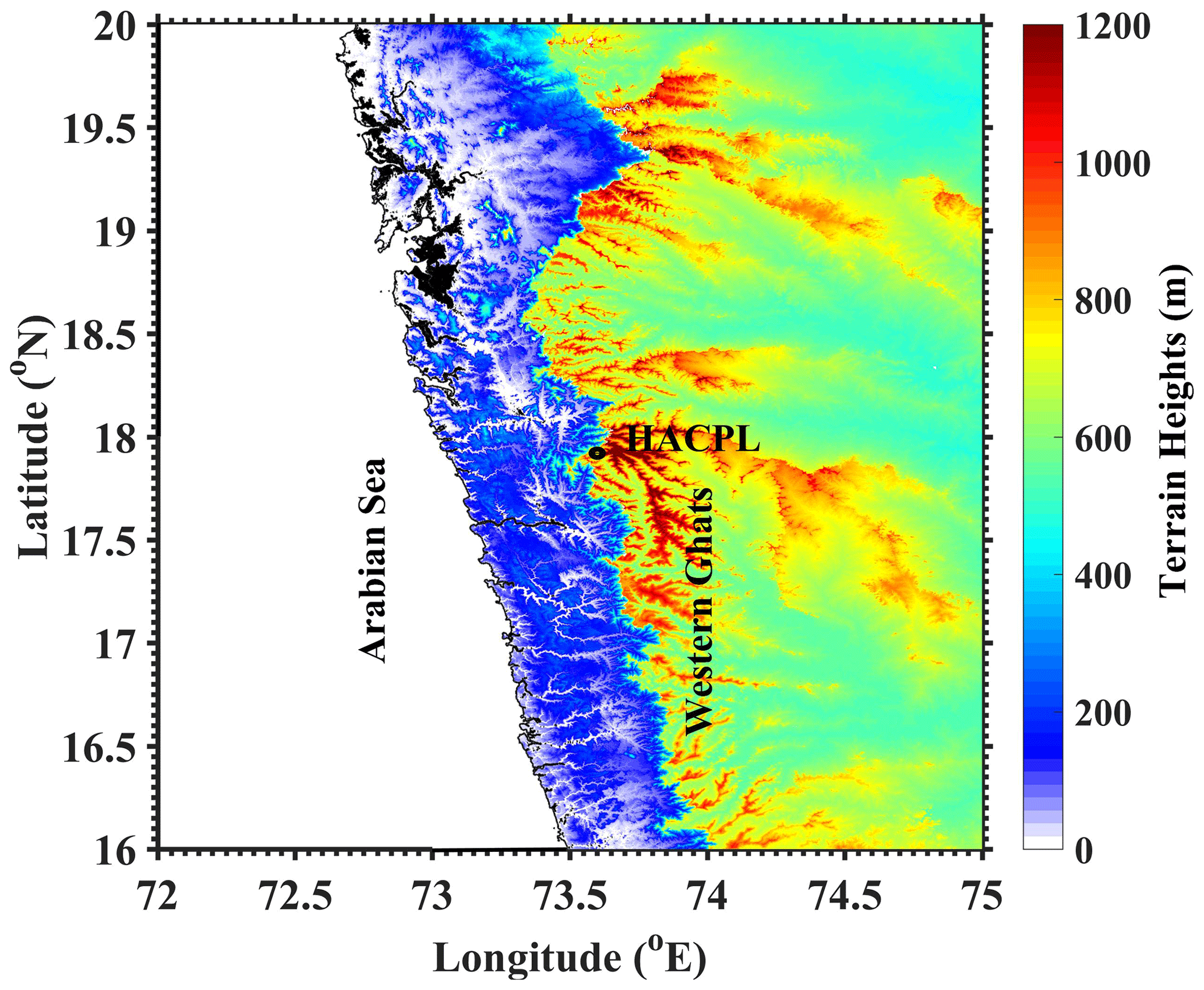
Figure 1Topographical map of India's Western Ghats generated by using Shuttle Radar Topography Mission (SRTM) data (Farr et al., 2007). The location of the disdrometer installed at HACPL is shown with a black circle.
A JWD is an impact-type disdrometer, which measures hydrometeors with sizes ranging from 0.3 to 5.1 mm and arranges them in 20 channels (Joss and Waldvogel, 1969). The JWD has a styrofoam cone to measure the diameter of hydrometeors. Once the hydrometeors hit the 50 cm2 styrofoam cone, a voltage is induced by downward displacement, which is directly correlated with drop size. The accuracy of the JWD is 5 % of the measured drop diameter. Although a JWD is a standard instrument for DSD measurements (Tokay et al., 2005), it has several shortcomings, such as noise, sampling errors, and wind (Tokay et al., 2001, 2003). In addition, the JWD miscounts raindrops in lower-sized bins, specifically for drop diameters below 1 mm (Tokay et al., 2003). Effort has been made to overcome this deficiency by discarding noisy measurements and applying the manufacturer's error correction matrix. To reduce the sampling error arising from insufficient drop counts, rain rates less than 0.1 mm h−1 are discarded. During heavy rain, the JWD underestimates the number of smaller drops; this is known as disdrometer dead time. To account for the aforementioned error in JWD estimates, the rain rates during wet and dry spells are analyzed. It is observed that ∼85 % (90 %) of the rain rates lie below 8 mm h−1 during wet (dry) spells (figure not shown). Using the noise-limit diagram of Joss and Gori (1976), Tokay et al. (2001) investigated the underestimation of small drops by the JWD. They found that 50 % of the drops below 0.4 mm cannot be detected by the JWD when the rain rate is above 20 mm h−1. Here, only 4 % (1 %) of the rain rates exceed 20 mm h−1 during wet (dry) spells, and hence the underestimation of small drops by the JWD is negligible in this region. Tokay et al. (2001) further demonstrated that the gamma parameters (such as a normalized intercept parameter) derived from long-term observations by a JWD and a two-dimensional video disdrometer (2DVD) are in good agreement. We examined the DSD differences between the ISM's wet and dry spells using a long-term (four monsoon) dataset in the present study. So it is appropriate that the undercounting of small drops does not significantly affect the gamma DSD. Further, the underestimation of smaller drops for higher rain rates (4 % for wet spells and 1 % for dry spells) may not affect the conclusions, as this work does not intend to quantify the DSD variations. Instead, it aims to understand the DSD variability during wet and dry spells over the complex terrain. The undersized integration period can contribute to DSD's numerical fluctuations, whereas a longer sampling time may miscount actual physical deviations (Testud et al., 2001). As there is no consensus regarding the JWD sampling period, we have averaged the JWD measurements into 1 min periods to filter out these deviations.
A JWD provides rain integral parameters, like raindrop concentration, rain rate, and reflectivity, at 1 min integration time (Krishna et al., 2016; Das et al., 2017). The 1 min DSD measurements are fitted with a three-parameter gamma distribution, as mentioned in Ulbrich (1983). Details of the DSDs used in the present study can be found in Das et al. (2017) and Murali Krishna et al. (2017).
The functional form of the gamma distribution assumed for DSD is expressed as
where N(D) is the number of drops per unit volume per unit size interval, N0 (in m−3 mm) is the number concentration parameter, D (in mm) is the drop diameter, D0 (in mm) is the median volume diameter, and μ (unitless) is the shape parameter (Ulbrich, 1983; Ulbrich and Atlas, 1984). The gamma DSD parameters are calculated using moments proposed by Cao and Zhang (2009). Here, second, third, and fourth moments are utilized to estimate gamma parameters. This method gives relatively fewer errors than other methods over the WG (Konwar et al., 2014). The nth-order moment of the gamma distribution can be calculated as
The shape parameter, μ, and the slope parameter, λ, are expressed as
The other parameters, including the normalized intercept parameter Nw (in ), mass-weighted mean diameter Dm (in mm), and liquid water content (LWC; in gm m−3), are calculated following Bringi and Chandrasekar (2001).
Here, ρw is the density of water.
Apart from JWD measurements, the ERA-Interim (Dee et al., 2011) dataset is also used to understand the dynamical processes influencing different DSD characteristics. ERA-Interim provides atmospheric data at different pressure and time intervals. Here, temperature (K), specific humidity (kg kg−1), and horizontal and vertical winds at 850 hPa with a spatial resolution of at 00:00 UTC are considered during the ISM period of 2012–2015.
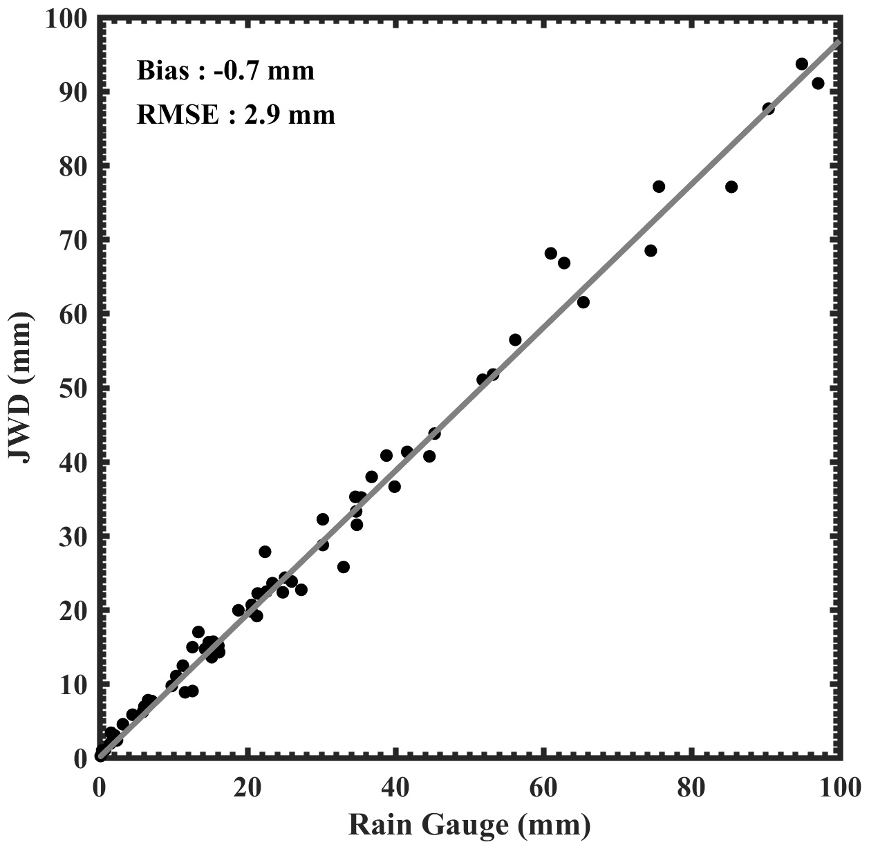
Figure 2Scatter plot of daily accumulated rainfall between the rain gauge and the JWD. The solid grey line indicates the linear regression.
The daily accumulated rainfall collected by the India Meteorological Department (IMD) rain gauges is used to identify ISM's wet and dry spells. IMD receives the rainfall accumulations at 08:30 LT ( h) every day. To examine JWD data quality, the daily accumulated rainfall measured by the JWD is compared with the daily accumulated rainfall collected from a rain gauge. For comparison, JWD rainfall accumulated at 08:30 LT is calculated for all the days during the 2015 monsoon. The daily accumulated rainfall collected by the rain gauge and the JWD above 1 mm is considered for the comparison. A total of 76 d of data are utilized. Non-availability of data might occur either due to maintenance activity or due to non-rainy days. Figure 2 shows the scatter plot of daily accumulated rainfall between the JWD and the rain gauge. The correlation coefficient is about 0.99 between the two measurements despite their different physical and sampling characteristics. The JWD measured rainfall bias is about −0.7 mm, and the root mean square error is about 2.9 mm. These results suggest that the JWD measurements can be utilized to understand the DSD characteristics during wet and dry spells of the ISM in the WG region.
Pai et al. (2014) proposed an objective methodology to identify wet and dry spells of the ISM. A long-term (1979–2011), high-resolution () gridded daily rainfall dataset from the IMD rain gauge network is used to classify the wet and dry spells of the ISM. The area-averaged daily rainfall time series is constructed for HACPL in the Mahabaleshwar (17.75–18∘ N and 73.5–73.75∘ E) region during the monsoon (1 June to 30 September) for 4 years (2012–2015) as well as for long-term data. The daily average rainfall difference for four monsoons and the daily average of the long-term data provide the daily anomalies. The standard deviation of daily average rainfall is calculated from long-term data. The standardized anomaly time series is obtained by normalizing the daily anomalies with corresponding standard deviations.
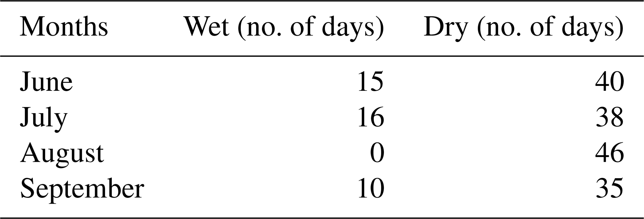
These standardized anomaly time series are used to separate the wet and dry spells. A period in this time series is marked as wet (dry) if the standardized anomaly exceeds 0.5 (−0.5) for three consecutive days or more (Utsav et al., 2019). Figure 3 shows the standardized rainfall anomalies calculated using Eq. (9). Table 1 shows the number of wet and dry days for the study period. It is observed that there are more dry days during the 2012–2015 monsoon, and July has relatively more wet days. A total of 44 640 (149 760) 1 min raindrop spectra are analyzed during wet (dry) days for the 2012–2015 ISM.
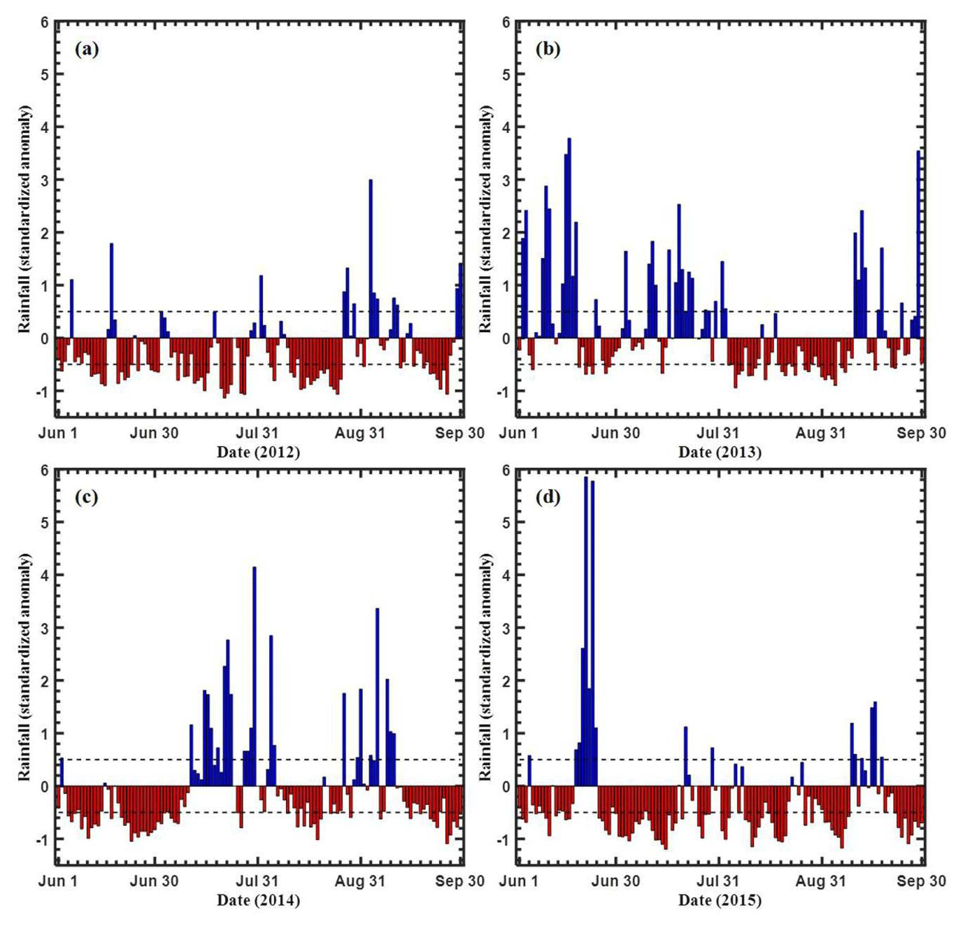
Figure 3The standardized rainfall anomaly for the years (a) 2012, (b) 2013, (c) 2014, and (d) 2015 during June–September. The dashed line marks the 0.5 and −0.5 rainfall anomaly.
Table 1Total number of wet and dry days during the monsoon (June–September) of 2012–2015.
A single pointwise instrument is not sufficient to address the orographic impacts on DSD characteristics. One of the difficulties in studying the effect of orography on DSD properties is the unavailability of many disdrometer measurements in the WG region. Here an overview of DSD characteristics over the WG is shown using Global Precipitation Measurement (GPM) mission satellite products. The GPM level 3 data provide different DSD parameters like Dm and Nw at a spatial resolution of from 60∘ S to 60∘ N. The GPM is the first spaceborne dual-frequency precipitation radar (DPR) that contains the Ku-band at ∼13.6 GHz and Ka-band at ∼35.5 GHz. The details of the GPM mission can be found in Huffman et al. (2015), and the dataset used can be found in Murali Krishna et al. (2017).
The GPM estimates Dm and Nw using the dual-frequency ratio (DFR) method. However, the GPM DPR suffers from limitations. The DSD parameterization used in the GPM DPR is the gamma distribution with a constant shape parameter, μ=3 (Liao et al., 2014). The constant μ introduces errors into the retrievals. The retrieval of Dm using the DFR method is iterative, and it has two solutions when the DFR is less than 0 (Meneghini et al., 1997; Liao et al., 2003; Mardiana et al., 2004). The uncertainties in GPM DPR in estimating DSD are detailed in Seto et al. (2013) and Liao et al. (2014). Murali Krishna et al. (2017) assessed the DSD measurements from the GPM in the WG region by comparing them with a ground-based disdrometer. They showed that the seasonal variations in Dm and Nw are well represented in the GPM measurements. However, the GPM underestimates Dm and overestimates Nw compared to the ground-based disdrometer. Radhakrishna et al. (2016) also showed that the GPM underestimates (overestimates) the mean Dm (Nw) during southwest and northeast monsoons over Gadanki, a semiarid region of southern India. They showed that the single-frequency algorithm underestimates mean Dm by ∼0.1 mm below 8 mm h−1, and the underestimation is a little higher at higher rain rates, whereas in the DFR algorithm, the mean Dm is nearly the same below 8 mm h−1 but underestimated (∼0.1 mm) at higher rain rates. Further, the underestimation is very small for Dm below 1.5 mm. In most cases, the rainfall intensity is below 8 mm h−1 (as discussed in the previous section), and Dm is below 1.5 mm in the WG region. Hence, it is reasonable to consider the GPM measurements to present DSD characteristics over the WG.
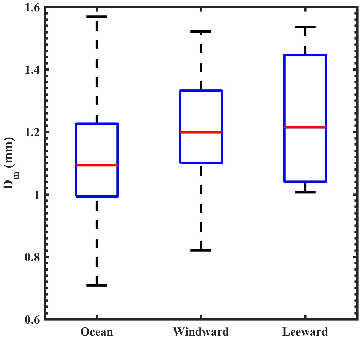
Figure 4Box-and-whisker plot of Dm distributions over the ocean, windward side (HACPL), and leeward side of the mountain from GPM measurements. The box represents the data between the first and third quartiles, and the whiskers show the data from the 12.5 and 87.5 percentiles. The horizontal line within the box represents the median value of the distribution.
Three locations (ocean, windward side, and leeward side of WG) are selected to examine the DSD variations in different topographic regions. The DSD differences at these three sites can be used to partly infer the effect of orography on DSD. Figure 4 shows the Dm distribution over the ocean, windward side, and leeward side of the WG. The Dm distribution is smaller over the ocean and windward side, whereas Dm shows large variability on the leeward side. Further, the Dm median value is lower over the ocean than the windward and leeward sides of the mountain. The smaller distribution of Dm over the ocean and windward side can be attributed to shallow clouds and cumulus congestus. The broader distribution and relatively higher median value of Dm represent the continental convection on the mountain's leeward side. Zagrodnik et al. (2019) also observed the narrow Dm distribution during the Olympic Mountains Experiment (OLYMPEX) on the Olympic peninsula's windward side.
The DSD and rain integral parameters during wet and dry spells are examined in terms of the diurnal cycle and with different types of precipitation (convective and stratiform). We considered raindrops with diameters less than 1 mm to be small drops, diameters between 1 and 4 mm to be midsize drops, and diameters above 4 mm to be large drops.
5.1 Raindrop size distribution during wet and dry spells
Figure 5 shows the temporal evolution of the normalized raindrop concentration during wet and dry spells for smaller and midsize drops. The concentration of smaller drops (Fig. 5a) is higher during dry periods. The higher concentration of small drops in dry spells indicates the influence of orography on rainfall over the WG. In the mountain regions rainfall is produced when the upslope wind is stronger and moisture availability is high (White et al., 2003). In such a situation, the strong orographic wind enhances cloud droplet growth via condensation, collision, and coalescence (Konwar et al., 2014). Further, many small raindrops during dry spells indicate drop breakup and evaporation processes. For smaller drops, dry spells exhibit a strong diurnal cycle with a primary maximum in the afternoon (15:00–19:00 LT) and a secondary peak in the night (23:00–05:00 LT). Utsav et al. (2019) also found similar diurnal features in 15 dBZ echo-top height (ETH) from radar observations during dry spells. However, such a diurnal cycle is not present in smaller drops during wet spells. These smaller drops show a slightly higher concentration during morning (05:00–07:00 LT), representing the oceanic nature of rainfall (Narayana Rao et al., 2009; Krishna et al., 2016).
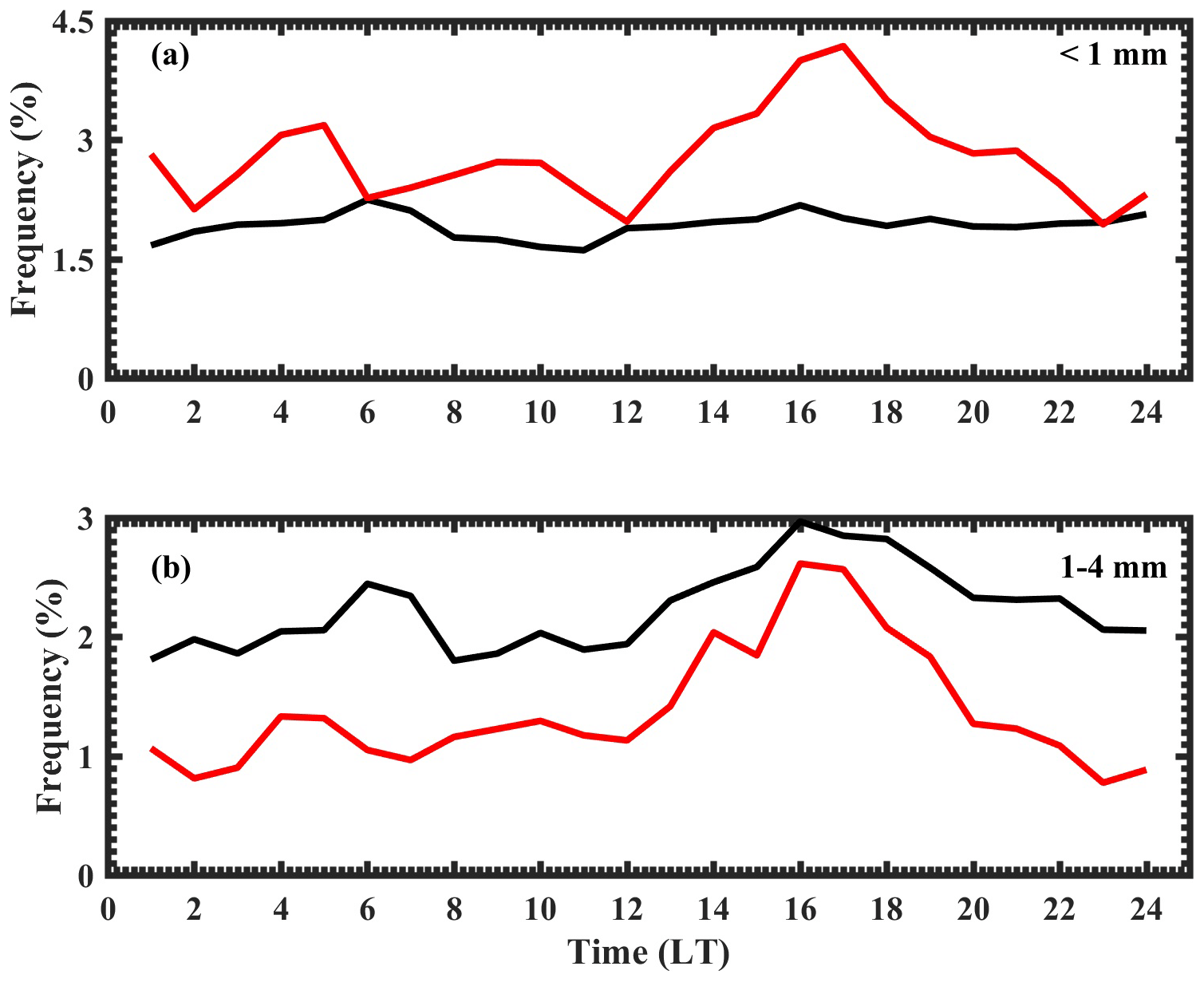
Figure 5Diurnal variation in raindrop concentration during wet and dry spells for (a) smaller drops (<1 mm) and (b) midsize drops (1–4 mm). The concentration of raindrops within each hour is normalized with the total concentration of raindrops in the respective spells (wet or dry). The black line represents wet spells, and the red line represents dry spells.
For midsize drops (Fig. 5b), the concentration is higher in wet spells than dry spells. The higher concentration of midsize drops during wet spells could be due to the collision–coalescence process (Rosenfeld and Ulbrich, 2003) and accretion of cloud water by raindrops (Zhang et al., 2008). This result suggests that congestus clouds are omnipresent during wet spells. A clear diurnal cycle can be observed during both spells; however, their strengths are different. The wet spells exhibit two broad maxima, one in the late afternoon (14:00–19:00 LT) and the other in the early morning (05:00–07:00 LT). The dry spells also show two maxima, one in the late afternoon (14:00–19:00 LT) as in the wet periods, and the other in the night (23:00–05:00 LT). Such a diurnal cycle is also observed in rainfall features over the WG (Shige et al., 2017; Romatschke and Houze, 2011). Shige et al. (2017) found continuous rainfall with a double-peak structure of nocturnal and afternoon–evening maxima in the WG region. Romatschke and Houze (2011) observed a double-peak rainfall pattern in the WG region. They proposed that the morning peak is related to oceanic convection, while the afternoon peak is associated with continental convection.

Figure 6 shows the mean DSDs during wet and dry spells along with the seasonal mean. Here, N(D) is plotted on a logarithmic scale to accommodate its large variability. In general, the DSDs during dry spells are narrower than during wet periods. The DSDs are concave-downward during both spells. The mean concentration of smaller drops (below 0.9 mm) is higher and the mean concentration of medium and larger drops is lower in dry periods. An increased concentration of smaller drops and a decrease in the number of medium and larger drop concentrations are found in the dry spells compared to the seasonal mean concentration. This indicates the collision and breakup processes described by Rosenfeld and Ulbrich (2003) and Konwar et al. (2014). In contrast, low concentrations of smaller drops and an increase in the number concentration of drops above 0.9 mm diameter are observed in the wet spells.
To study the differences in DSD during wet and dry spells with rain rate, the N(D) distribution is compared at different rain rates, as shown in Fig. 7. Here, N(D) is plotted on a logarithmic scale. A significant difference in N(D) is found between wet and dry spells. The contours are shifted to higher rain rates and higher diameters in the wet spells. This indicates that the number of midsize drops in the range 1–2 mm is higher in wet spells than in dry spells for the same rain rate. This is more pronounced at lower rain rates below 10 mm h−1. Further, the raindrop concentration in the range 1–2 mm increases as the rain rate increases between 5 and 15 mm h−1 during wet periods. At higher rain rates (above 10 mm h−1), the number of smaller and midsize drops is higher in the wet spells than in the dry periods. However, this difference decreases gradually as the rain rate increases. At above 30 mm h−1, both the periods show a similar distribution of N(D) (not shown). However, for larger drops above 4.5 mm, the concentration is higher in wet spells than dry periods for all rain rate intervals (not shown).
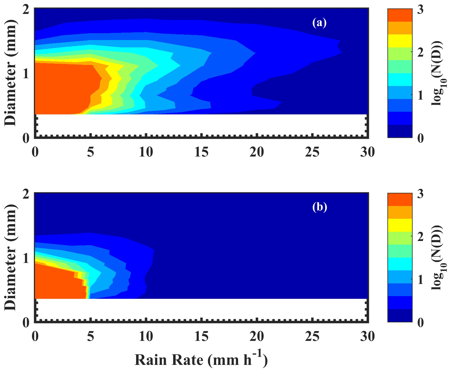
Figure 7The variation in N(D) as a function of D at different rain rates for (a) wet and (b) dry spells.
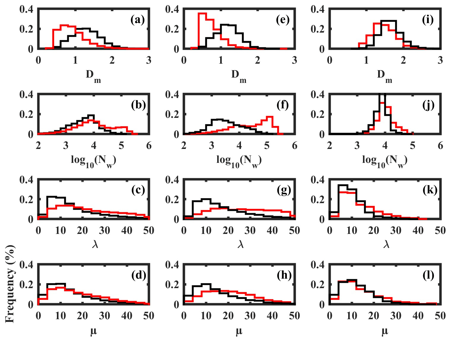
Figure 8Histograms of (a) Dm, (b) log 10(Nw), (c) λ, and (d) μ for wet and dry spells. (e–h) Same as (a–d), but for stratiform rain. (i–l) Same as (a–d), but for convective rain. Here, the black and red lines represent wet and dry spells, respectively.
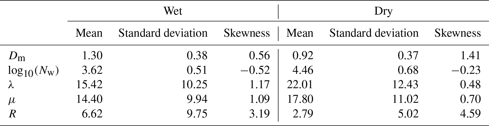
Figure 8 presents histograms of Dm, log 10(Nw), λ, and μ during wet and dry spells. The histograms of Dm are positively skewed during both wet and dry periods (Fig. 8a). The distribution of Dm is broader in dry spells. The Dm varies from 0.42 to 4.8 mm, with a maximum at ∼1.2 mm during wet periods, whereas it ranges from 0.4 to 5 mm, with a maximum at ∼0.8 mm during dry spells. For Dm below 1 mm, the dry spell distribution is higher than for wet spells. This finding indicates the predominance of smaller drops during dry spells. The mean, standard deviation, and skewness of Dm are provided in Table 2. The mean Dm is 1.3 mm, and its standard deviation is 0.38 during wet spells, whereas the mean Dm is 0.9 mm, and its standard deviation is 0.37 during dry spells. A relatively large number of small drops reduce Dm in dry spells, while fewer smaller drops and relatively more midsize drops increase Dm in wet periods. The histograms of log 10(Nw) are negatively skewed during both wet and dry spells (Fig. 8b). The log 10(Nw) shows an inverse relation with Dm and is varied from 0.52 to 5.11 during wet spells and from 0.50 to 5.43 during dry periods. The histogram of log 10(Nw) peaks at 3.9 during wet periods; however, it shows a bimodal distribution during dry spells that peaks at 3.9 and 5. This finding is consistent with Utsav et al. (2019). They analyzed 0 dBZ ETH, which represents the cloud-top height, and observed a bimodal distribution, which peaks at 3 and 6.5 km during dry periods. The large standard deviation indicates the large variations in Dm and Nw during both wet and dry periods. The histograms of λ and μ are shown in Fig. 8c and d. Generally, λ represents the truncation of the DSD tail and μ indicates the breadth of DSD. If λ is small, the DSD tail is extended to larger diameters and vice versa. The positive (negative) μ indicates the concave-downward (upward) shape for the DSD. The zero value of μ represents the exponential shape for DSD (Ulbrich, 1983). The λ shows positive values during wet and dry spells. The occurrence of λ is higher below 10 mm−1 during wet periods, indicating the broader spectrum of raindrops, whereas it is distributed up to 20 mm−1 during dry spells. The extension of λ towards higher values represents the higher occurrence of smaller drops during both periods. Relatively smaller λ and Nw in wet spells indicate that the tail of DSD extends to large raindrop sizes. The μ is positive during both wet and dry spells, indicating the concave-downward shape of DSD.
Table 2Mean, standard deviation, and skewness of the DSD parameters in wet and dry spells.
Numerous studies have been carried out to understand DSDs during different types of convection and within a convective system (Dolman et al., 2011; Munchak et al., 2012; Friedrich et al., 2013; Thompson et al., 2015; Dolan et al., 2018). These studies showed that the combined dynamical (stratiform and convective) and microphysical processes occurring in a precipitating system cause differences in observed DSD. Therefore, to understand the effect of dynamical processes on different DSD characteristics during wet and dry spells, the precipitation events are classified into stratiform and convective types. Several rain classification schemes are proposed in the literature using different instruments, like a disdrometer, radar, and/or a profiler (Bringi et al., 2003; Thompson et al., 2015; Krishna et al., 2016; Das et al., 2017; Dolan et al., 2018; Nair, 2019). In this work, precipitating systems are classified as stratiform and convective based on the Bringi et al. (2003) criterion. Even though several other classification schemes are in the literature, it is the most widely used classification criterion for stratiform and convective rainfall. The main purpose here is to understand the DSD differences between convective and stratiform (rain that does not fall under the convective category) rain systems. For rain type classification, Bringi et al. (2003) considered five consecutive 2 min DSD samples. However, 10 successive 1 min DSD samples are considered to classify rainfall as stratiform and convective in this work. If the mean rain rate of 10 successive DSD samples is greater than 0.5 mm h−1 and if the standard deviation is less than 1.5 mm h−1, then the precipitation is classified as stratiform; otherwise, it is classified as convective.
Table 3Mean, standard deviation, and skewness of the DSD parameters in stratiform rain for wet and dry spells.
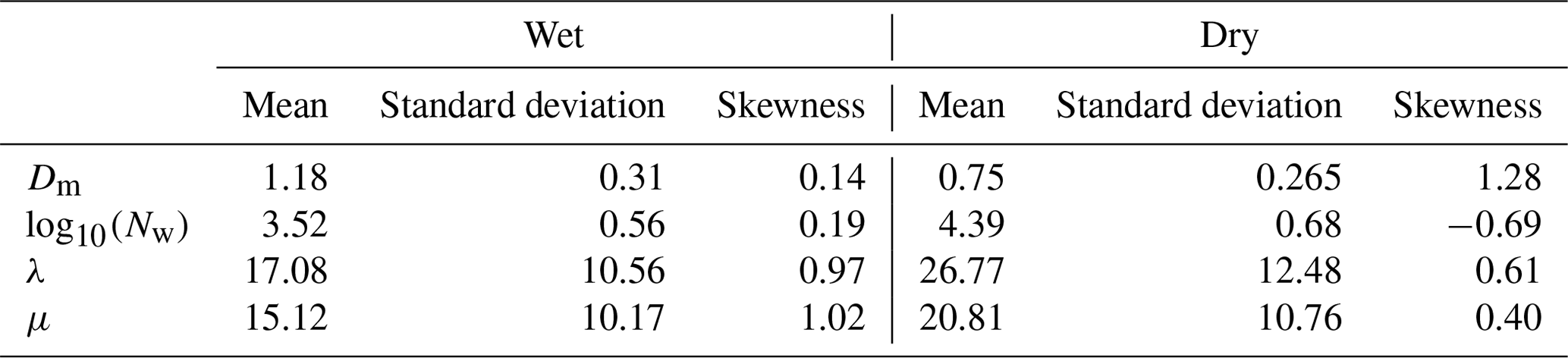
Figure 8e–h present histograms of Dm, log 10(Nw), λ, and μ during stratiform rain events in wet and dry spells. The mean, standard deviation, and skewness of these parameters are provided in Table 3. The histograms of Dm (Fig. 8e) are positively skewed during stratiform rain events in both the spells. The Dm is broader in stratiform rain for dry spells, and it varies between 0.38 and 2.77 mm with a maximum near 0.42–0.58 mm. The distribution of Dm shows higher frequency below 0.6 mm in dry spells. This finding indicates the presence of more smaller raindrops in stratiform rain for dry spells. The Dm varies from 0.42 to 2.48 mm with a maximum near 1–1.4 mm during stratiform rain in wet periods. The Dm distribution is higher in wet spells above 1 mm, indicating the dominance of midsize and/or larger drops. The histogram of log 10(Nw) (Fig. 8f) is positively skewed in the wet spells and negatively skewed in the dry periods for stratiform rain. The distribution is narrower in wet periods and broader in dry spells. The distribution peaks between 3 and 3.6 during wet spells, whereas it peaks at 5 during dry spells. The distribution of λ (Fig. 8g) is broader in stratiform rain events during both wet and dry periods. The distribution varies from 1.2 to 52 mm−1 with a mode at 10 mm−1 in stratiform rain for wet spells. This result further supports the presence of midsize drops in wet periods. The distribution of λ shows higher occurrences above 15 mm−1 during dry spells, indicating the truncation of DSD at relatively smaller drop diameters. The histograms of μ (Fig. 8h) show a concave-downward shape for DSDs during stratiform rain events in both wet and dry spells.
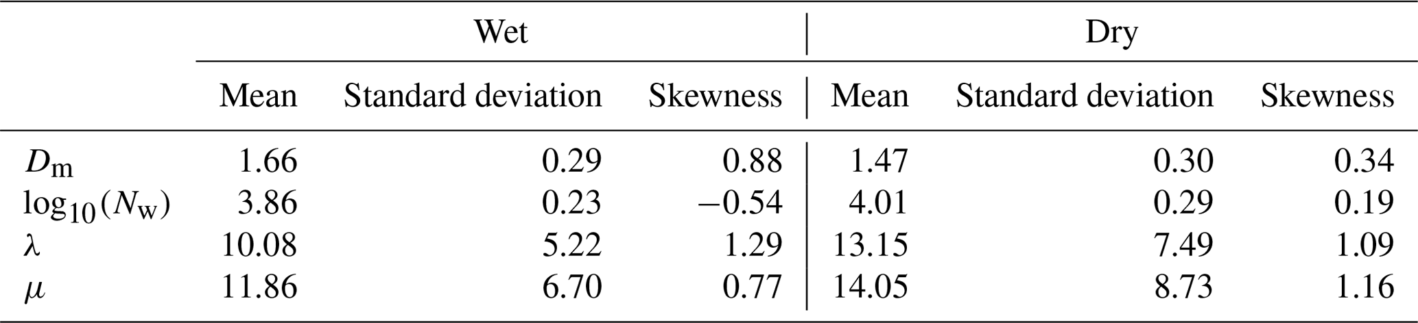
Figure 8i–l show the distribution of Dm, log 10(Nw), λ, and μ during convective rain events in wet and dry spells. The Dm histograms are positively skewed in convective rain during both wet and dry spells (Fig. 8i). In convective rain, the distribution of Dm is broader in wet spells. It can be seen that the presence of small drops is higher in dry spells, even in convective rain. The distribution of log 10(Nw) shows an inverse relation with Dm in convective rain (Fig. 8j). The log 10(Nw) is negatively skewed in wet spells, whereas it is positively skewed in dry spells. The distribution of λ (Fig. 8k) indicates larger drops in convective rain compared to stratiform rain in both wet and dry spells. The histograms of μ (Fig. 8l) show the concave-downward shape of DSDs in convective rain for both wet and dry spells. The mean, standard deviation, and skewness of these parameters are provided in Table 4.
Table 4Mean, standard deviation, and skewness of the DSD parameters in convective rain for wet and dry spells.
Several points can be noted from the above discussion.
- a.
The maximum value for mean Dm and the largest standard deviation are for convective rain in wet spells.
- b.
The maximum value for log 10(Nw) and higher standard deviation are observed during stratiform rain in dry spells.
- c.
A considerable difference is found in Dm and log 10(Nw) during stratiform rain in dry and wet periods. However, this difference is small in convective rain.
- d.
There are distinct differences in λ and μ for stratiform rain during wet and dry spells.
The above results indicate that rainfall over the WG is associated with warm rain processes during wet and dry spells. The microphysical processes in warm rain include rain evaporation, accretion of cloud water by raindrops, and rain sedimentation (Zhang et al., 2008). Giangrande et al. (2017) observed the predominance of larger cloud droplets in warm clouds during wet spells over the Amazon. Similarly, Machado et al. (2018) showed that larger Dm is associated with mixed-phase clouds during dry periods over the Amazon. Recently, Utsav et al. (2019) showed that cumulus congestus is higher during wet spells, and shallow clouds are dominant during dry periods in the WG region. Thus, the larger Dm may be due to cumulus congestus during wet spells. The differences in Dm during wet and dry spells might occur at the cloud formation stage and/or during the descent of precipitation particles to the ground. The microphysical and dynamical processes during the descent of precipitation particles are responsible for the spatial–temporal variability in Dm (Rosenfeld and Ulbrich, 2003). The dominant dynamical processes that affect Dm are updrafts, downdrafts, and advection by horizontal winds. To understand the dynamical mechanisms leading to different microphysical processes during wet and dry periods, we have analyzed temperature, specific humidity, and horizontal and vertical winds for the 2012–2015 monsoon. Figure 9 shows the anomalies in specific humidity (kg kg−1, shading), temperature (K, contours), and horizontal winds (vectors) at 850 hPa derived from the ERA-Interim dataset. This pressure level is selected, as the temperature anomaly and moisture availability aid the growth of active convection. The daily 00:00 UTC ERA-Interim data for 10 years (2006–2015) are considered to find anomalies. Seasonal averages are calculated for different atmospheric parameters, and the anomalies are estimated as the difference between the wet and dry period mean and the seasonal mean. Here, positive anomalies in specific humidity (temperature) represent an increase in moisture content (heating), and a negative anomaly represents a decrease in specific humidity (cooling). It is observed that the temperature over the west coast of India (including the study region) is cooler in wet spells than dry periods. This figure also shows that the anomalous winds are maritime and continental during wet and dry spells, respectively. The anomalous winds coming from the oceanic region bring more moisture (positive anomalies in specific humidity) over the WG during wet spells, whereas the anomalous winds coming from the continent bring dry (negative anomalies in specific humidity) air during dry spells. The thermal gradient between the WG and surrounding regions and the availability of more moisture favor active convection in the wet spells, whereas positive temperature anomalies in the dry spell can lead to evaporation of raindrops, which can subsequently break the drops, thereby leading to smaller-diameter drops.
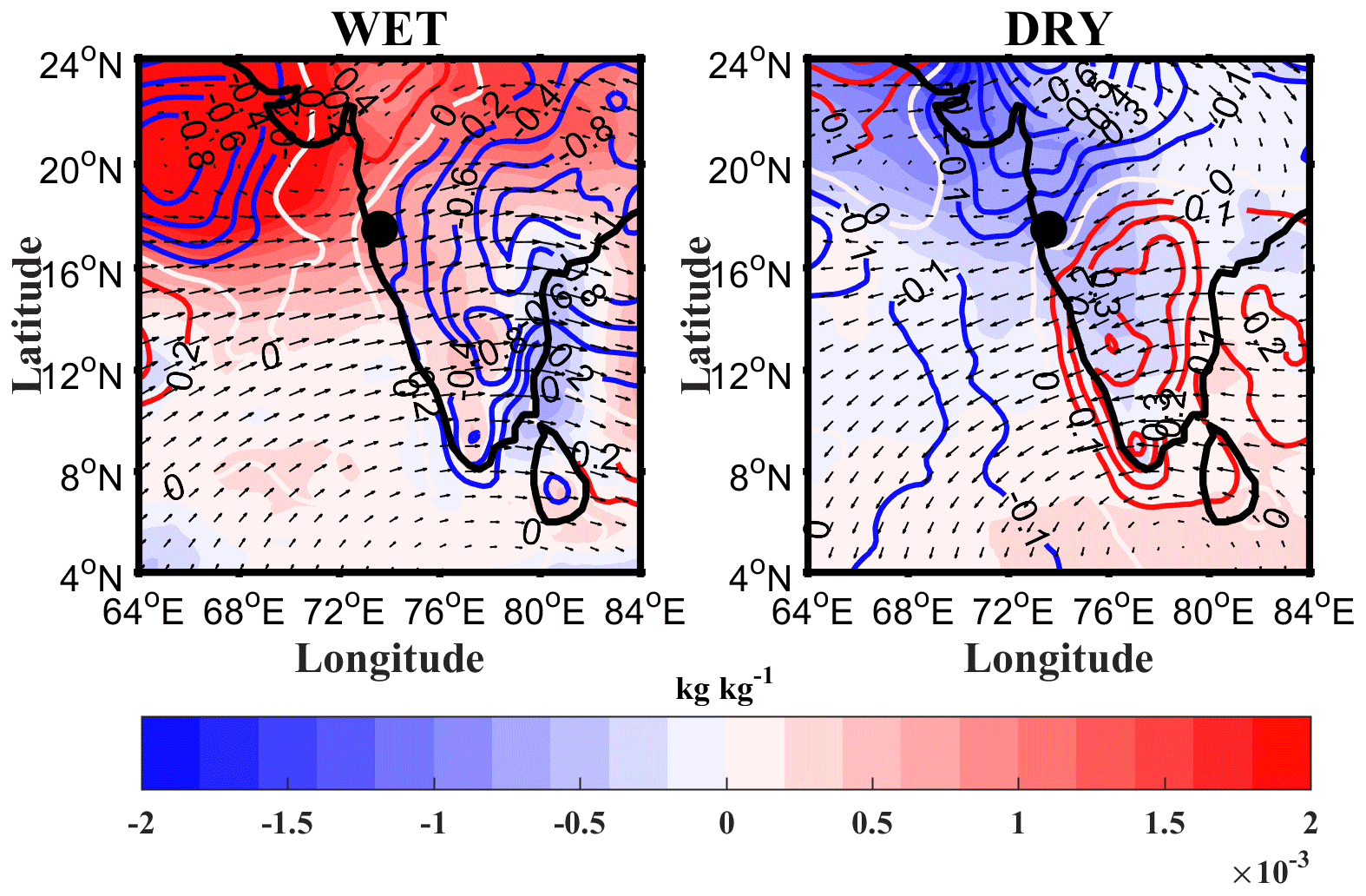
Figure 9Spatial distribution of anomalies in specific humidity (kg kg−1, shading), temperature (K, contours), and horizontal winds (vectors) at 850 hPa during wet and dry spells in the monsoon for 2012–2015. Here, positive anomalies in specific humidity (temperature) represent an increase in moisture content (heating), and a negative anomaly represents a decrease in moisture (cooling). The black dot represents the observational site.
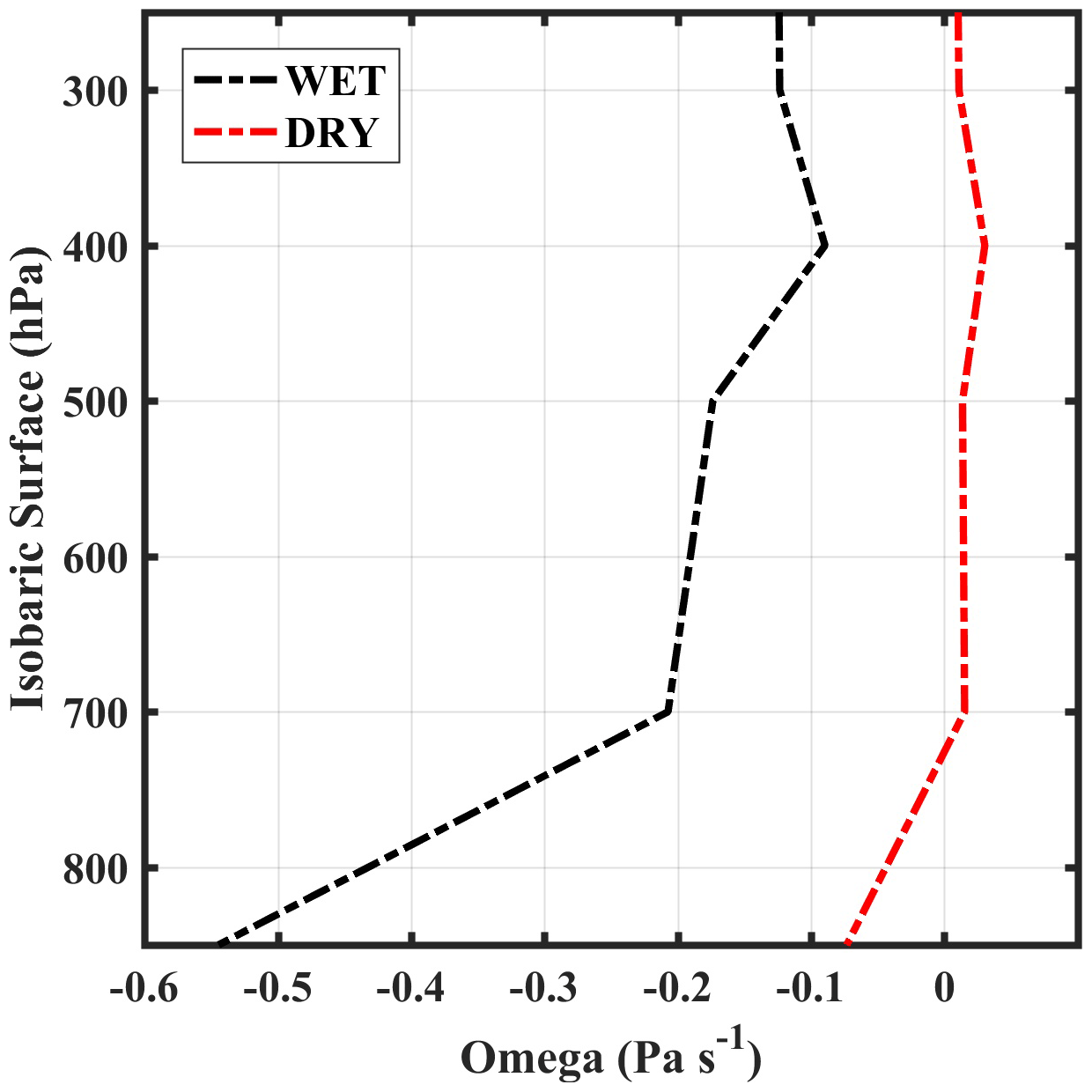
To understand the effect of updrafts and downdrafts on Dm variability, the omega (vertical motion in pressure coordinates) field is analyzed for the region 17–18∘ N and 73–74∘ E. Figure 10 shows the vertical profile of omega during wet and dry spells. Here, negative values of omega represent updrafts and vice versa. The mean vertical winds are negative in wet spells, indicating updrafts, whereas the mean vertical winds are small and positive, indicating downdrafts during dry spells. The updrafts do not allow the smaller drops to fall, which are carried aloft, where they can fall out later. Hence, the smaller drops have enough time to grow through the collision–coalescence process to form midsize or large-size drops. Therefore, medium- or large-size drops increase at the expense of smaller drops, which leads to larger Dm during wet spells, whereas the downward flux of raindrops increases due to the downdrafts, which causes smaller drops to reach the surface. The large density of smaller drops decreases Dm during dry spells.
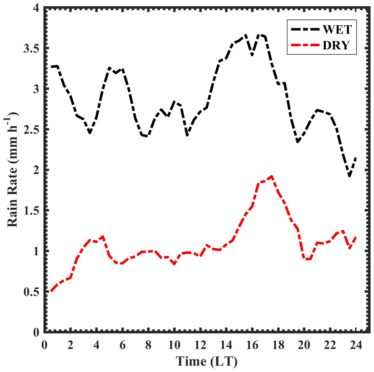

Figure 12Distribution of Dm at different rain rates for wet and dry spells. The horizontal line within the box represents the median value. The boxes represent data between the first and third quartiles, and the whiskers show data from the 12.5 to 87.5 percentiles. Black represents wet spells, and red represents dry spells.

The diurnal variation in the mean rain rate during wet and dry spells is shown in Fig. 11. The mean rain rate is higher during wet periods throughout the day. The relatively lower rain rates are due to a higher concentration of smaller drops during dry spells. The diurnal variation in the rain rate shows a bimodal distribution during both wet and dry spells. The primary maximum is in afternoon hours and the secondary maximum is during morning hours. The raindrop concentration increases monotonically (refer Fig. 5), with an increase in rain rate for all the drop sizes during dry spells. This finding indicates that the increase in the rain rate is responsible for the rise in both the concentration and raindrop size during dry spells. However, in wet periods, the concentration of smaller drops is constant throughout the day, and the increase in rain rate is due to the rise in the concentration and size of midsize raindrops. This further indicates that the collision and coalescence processes and deposition of water vapor onto the cloud drops are responsible for the increased concentration (afternoon and early-morning hours) of midsize raindrops during wet spells. In addition, the raindrop diameter depends on the rain rate, which varies between wet and dry spells. The Dm distribution during wet and dry spells at different rain rates is shown in Fig. 12. The Dm is higher in wet spells than dry spells below 10 mm h−1. This could be due to the deposition of water vapor and accretion of cloud water on raindrops. This result in larger Dm during wet spells compared to dry spells. At higher rain rates (above 20 mm h−1), the Dm distribution remains the same during both spells. This is due to equilibrium of DSD by collision, coalescence, and breakup mechanisms, as described in Hu and Srivastava (1995) and Atlas and Ulbrich (2000). So, it is evident that the dynamical mechanisms underlying the microphysical processes cause the differences in DSD characteristics during wet and dry spells. The distinct DSD features during ISM's wet and dry spells over the WG are summarized in Fig. 13.
5.2 Implications of DSD during wet and dry spells: μ–λ relation
The gamma distribution is widely used in microphysical parameterization schemes in numerical models to describe various DSDs. However, μ is often considered to be constant. Milbrandt and Yau (2005) found that μ plays a vital role in determining sedimentation and microphysical growth rates. In this context, the microphysical properties of clouds and precipitation are sensitive to variations in μ. Several researchers showed that μ varies during the precipitation (Ulbrich, 1983; Ulbrich and Atlas, 1998; Testud et al., 2001; Zhang et al., 2001; Islam et al., 2012). Zhang et al. (2003) proposed an empirical μ–λ relationship using 2DVD data collected in Florida. They examined the μ–λ relation with different rain types. These μ–λ relations are useful in reducing the bias in estimating rain parameters from remote sensing measurements (Zhang et al., 2003). Recent studies have demonstrated variability in the μ–λ relation for different types of rain and geographical locations (Chang et al., 2009; Kumar et al., 2011; Wen et al., 2016). Hence, it is necessary to derive different μ–λ relations based on local DSD observations.
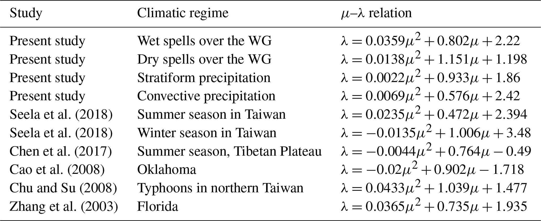
Seela et al. (2018)Seela et al. (2018)Chen et al. (2017)Cao et al. (2008)Chu and Su (2008)Zhang et al. (2003)Table 5Comparison of μ–λ relations derived in the present study with other orographic precipitation regions.
An empirical μ–λ relationship is derived for both wet and dry spells. The DSDs with a rain rate less than 5 mm h−1 are excluded to minimize the sampling errors. In addition, only total drop counts above 1000 are considered in the analysis, as proposed by Zhang et al. (2003). Figure 14 shows the μ–λ relation for wet and dry spells, and the corresponding polynomial least-square fits are shown as solid lines. The fitted μ–λ relations for wet and dry spells are given as follows.
The above equations represent the fact that the smaller the value of λ (higher rain rates), the smaller the value of μ in both spells. Thus, the DSDs tend to be more concave-downward with an increase in the rain rate. This finding suggests a higher fraction of small and midsize drops and a lower fraction of larger drops, reflecting less evaporation of smaller drops and more drop breakup processes. However, the fitted μ–λ relation exhibits a large difference between wet and dry spells. Comparing Eqs. (10) and (11), one can observe that the coefficient of the linear term is smaller in wet spells than that of dry spells. Hence, for a given μ, the dry spells have higher λ compared to the wet spells. Further, Dm is higher during wet spells than dry spells for a given rainfall rate due to the different microphysical mechanisms discussed above (Fig. 12). This leads to higher μ in wet spells than dry spells, which indicates that different microphysical mechanisms lead to different μ–λ relations. Hence, it is apparent that a single μ–λ relation cannot reliably represent the observed phenomenon during different monsoon phases.
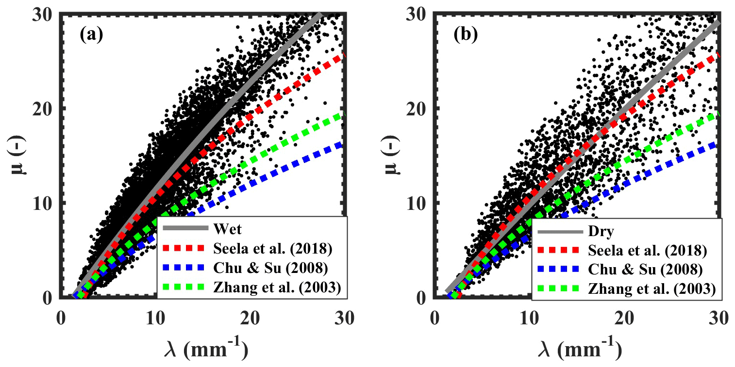
Figure 14Scatter plots of μ–λ values obtained from gamma DSD for (a) wet and (b) dry spells. The solid line indicates the least-square polynomial fit for the μ–λ relation.
Further, μ–λ relationships are derived for convective and stratiform rain as follows.
Seela et al. (2018) fitted μ–λ relations for summer and winter rainfall over northern Taiwan. Chen et al. (2017) derived an empirical μ–λ relation over the Tibetan Plateau. Cao et al. (2008) analyzed μ–λ relations over Oklahoma. Different μ–λ relations are derived for different weather systems over northern Taiwan (Chu and Su, 2008). The μ–λ relationship obtained in this work differs from Zhang et al. (2003), Chu and Su (2008), and Seela et al. (2018). The differences in μ–λ relations could be attributed to several factors like geographical location, microphysical processes, rain rate, and type of instrument. To explore the plausible effect of rainfall rate, μ–λ relations are compared with previous studies for rain rates below 5 mm h−1 (as in Chu and Su, 2008) and above 5 mm h−1 (as in Zhang et al., 2003) (figure not shown). It is observed that μ–λ relations in this work differ from previous studies at both rain rates. Further, the slope of the μ–λ relationship is higher over the WG than in previous studies. This shows that the wet and dry spells have a higher μ than previous studies for the same λ, indicating that the underlying microphysical processes are different over the complex orographic region of the WG. Further, Dm in the present study is higher than in previous studies (e.g., Seela et al., 2018). The different Dm distributions lead to different μ values (Ulbrich, 1983). Thus, relatively higher Dm values could contribute to higher μ for the same λ values in the present study. Hence, the differences in μ–λ relations compared to previous studies may be related to different rain microphysics (such as collision–coalescence, breakup). In addition, Zhang et al. (2003), and Chu and Su (2008) used 2DVD measurements, whereas JWD data are utilized in this work. The different instruments can have different sensitivities, which can also affect μ–λ relations. The μ–λ relationships derived for the current study are compared with the other orographic precipitation and are provided in Table 5. It is clear that μ–λ relations vary in different types of rainfall and climatic regimes.
The raindrop spectra measured by a JWD are analyzed to understand the DSD variations during wet and dry spells of the ISM over the WG. Observational results indicate that the DSDs are considerably different during wet and dry periods. In addition, the DSD variability is studied with stratiform and convective rain during wet and dry spells. Key findings are listed below.
- i.
A high concentration of smaller drops is always present in the WG region, indicating shallow convection dominance.
- ii.
The DSD over the WG shows distinct diurnal features. The dry spells exhibit a strong diurnal cycle with a double peak during late afternoon and nighttime for smaller and midsize drops, whereas this diurnal cycle is weak for smaller drops in wet spells.
- iii.
Small Dm and large Nw characterize the DSDs over the WG. The Nw shows a bimodal distribution during dry spells. This bimodality is weak in wet spells. The distribution of λ shows the dominance of small drops in dry spells and midsize drops in wet spells.
- iv.
The thermal gradient between the WG and surrounding regions, higher availability of water vapor, and strong vertical winds favor the formation of cumulus congestus, which are responsible for the presence of midsize to larger drops during wet spells.
- v.
The empirical relation between μ and λ shows a significant difference between wet and dry spells. The different microphysical mechanisms lead to different μ–λ relations.
It is evident from this study that, even though warm rain is predominant, the dynamical mechanisms underlying the microphysical processes are different, which causes the difference in observed DSD characteristics during wet and dry spells.
The disdrometer data are archived at IITM and are available from the corresponding author (skd_ncu@yahoo.com) for research collaboration. GPM and ERA-Interim datasets were respectively downloaded from https://pmm.nasa.gov/data-access/downloads/gpm (NASA, 2018) and https://apps.ecmwf.int/datasets/data/interim-full-daily/levtype=pl/ (Simarro, 2019).
UVMK and SKD designed, analyzed, and prepared the paper. SKD, UVMK, GSE, and UB proposed the methodology. GSE, SMD, and GP contributed to the discussion of the paper.
The authors declare that they have no conflict of interest.
The authors are thankful to the director at IITM for his support. The authors would like to acknowledge the technical and administrative staff of the High Altitude Cloud Physics Laboratory (HACPL), Mahabaleshwar, for maintaining the disdrometer. The authors acknowledge the India Meteorological Department (IMD) for the provision of the rainfall dataset. The authors also acknowledge JAXA (Japan) and NASA (USA) for providing GPM data (https://pmm.nasa.gov/data-access/downloads/gpm, last access: 30 November 2018). The authors would like to acknowledge the European Centre for Medium-Range Weather Forecasts (ECMWF) for providing the ERA-Interim dataset. The paper benefitted from comments and suggestions provided by the editor and the anonymous reviewers
This paper was edited by Jayanarayanan Kuttippurath and reviewed by two anonymous referees.
Atlas, D. and Ulbrich, C. W.: An observationally based conceptual model of warm oceanic convective rain in the tropics, J. Appl. Meteorol., 39, 2165–2181, 2000. a
Atlas, D., Ulbrich, C. W., Marks Jr., F. D., Amitai, E., and Williams, C. R.: Systematic variation of drop size and radar-rainfall relations, J. Geophys. Res.-Atmos., 104, 6155–6169, 1999. a
Bringi, V., Chandrasekar, V., Hubbert, J., Gorgucci, E., Randeu, W., and Schoenhuber, M.: Raindrop size distribution in different climatic regimes from disdrometer and dual-polarized radar analysis, J. Atmos. Sci., 60, 354–365, 2003. a, b, c
Bringi, V. N. and Chandrasekar, V.: Polarimetric Doppler Weather Radar: principles and applications, Cambridge University Press, Cambridge (MA), 2001. a
Cao, Q. and Zhang, G.: Errors in estimating raindrop size distribution parameters employing disdrometer and simulated raindrop spectra, J. Appl. Meteorol. Clim., 48, 406–425, 2009. a
Cao, Q., Zhang, G., Brandes, E., Schuur, T., Ryzhkov, A., and Ikeda, K.: Analysis of video disdrometer and polarimetric radar data to characterize rain microphysics in Oklahoma, J. Appl. Meteorol. Clim., 47, 2238–2255, 2008. a, b
Chang, W.-Y., Wang, T.-C. C., and Lin, P.-L.: Characteristics of the raindrop size distribution and drop shape relation in typhoon systems in the western Pacific from the 2D video disdrometer and NCU C-band polarimetric radar, J. Atmos. Ocean. Tech., 26, 1973–1993, 2009. a
Chen, B., Hu, Z., Liu, L., and Zhang, G.: Raindrop Size Distribution Measurements at 4500 m on the Tibetan Plateau During TIPEX-III, J. Geophys. Res.-Atmos., 122, 11–092, 2017. a, b
Chu, Y.-H. and Su, C.-L.: An investigation of the slope–shape relation for gamma raindrop size distribution, J. Appl. Meteorol. Clim., 47, 2531–2544, 2008. a, b, c, d, e
Das, S. K., Uma, K., Konwar, M., Raj, P. E., Deshpande, S., and Kalapureddy, M.: CloudSat–CALIPSO characterizations of cloud during the active and the break periods of Indian summer monsoon, J. Atmos. Sol.-Terr. Phy., 97, 106–114, 2013. a, b
Das, S. K., Konwar, M., Chakravarty, K., and Deshpande, S. M.: Raindrop size distribution of different cloud types over the Western Ghats using simultaneous measurements from Micro-Rain Radar and disdrometer, Atmos. Res., 186, 72–82, 2017. a, b, c, d, e, f, g, h, i
Das, S. K., Simon, S., Kolte, Y. K., Krishna, U. M., Deshpande, S. M., and Hazra, A.: Investigation of raindrops fall velocity during different monsoon seasons over the Western Ghats, India, Earth Space Sci., 7, e2019EA000956, https://doi.org/10.1029/2019EA000956, 2020. a
Dee, D. P., Uppala, S. M., Simmons, A. J., Berrisford, P., Poli, P., Kobayashi, S., Andrae, U., Balmaseda, M. A., Balsamo, G., Bauer, P., Bechtold, P., Beljaars, A. C. M., van de Berg, L., Bidlot, J., Bormann, N., Delsol, C., Dragani, R., Fuentes, M., Geer, A. J., Haimberger, L., Healy, S. B., Hersbach, H., Hólm, E. V., Isaksen, L., Kãllberg, P., Köhler, M., Matricardi, M., McNally, A. P., Monge-Sanz, B. M., Morcrette, J.-J., Park, B.-K., Peubey, C., de Rosnay, P., Tavolato, C., Thépaut, J.-N., and Vitart, F.: The ERA-Interim reanalysis: Configuration and performance of the data assimilation system, Q. J. Roy. Meteor. Soc., 137, 553–597, 2011. a
Deshpande, N. and Goswami, B.: Modulation of the diurnal cycle of rainfall over India by intraseasonal variations of Indian summer monsoon, Int. J. Climatol., 34, 793–807, 2014. a
Dolan, B., Fuchs, B., Rutledge, S., Barnes, E., and Thompson, E.: Primary modes of global drop size distributions, J. Atmos. Sci., 75, 1453–1476, 2018. a, b
Dolman, B. K., May, P. T., Reid, I. M., and Vincent, R. A.: Profiler retrieved DSD evolution in the tropics and mid-latitudes, preprints, 35th Conf. on Radar Meteorology, Pittsburgh, PA. Amer. Meteor. Soc., 8A.1., 2011. a
Farr, T. G., Rosen, P. A., Caro, E., Crippen, R., Duren, R., Hensley, S., Kobrick, M., Paller, M., Rodriguez, E., Roth, L., Seal, D., Shaffer, S., Shimada, J., Umland, J., Werner, M., Oskin, M., Burbank, D., and Alsdorf, D.: The shuttle radar topography mission, Rev. Geophys., 45, RG2004, https://doi.org/10.1029/2005RG000183, 2007. a
Friedrich, K., Kalina, E. A., Masters, F. J., and Lopez, C. R.: Drop-size distributions in thunderstorms measured by optical disdrometers during VORTEX2, Mon. Weather Rev., 141, 1182–1203, 2013. a
Gadgil, S. and Joseph, P.: On breaks of the Indian monsoon, J. Earth Syst. Sci., 112, 529–558, 2003. a, b
Gao, W., Sui, C.-H., Chen Wang, T.-C., and Chang, W.-Y.: An evaluation and improvement of microphysical parameterization from a two-moment cloud microphysics scheme and the Southwest Monsoon Experiment (SoWMEX)/Terrain-influenced Monsoon Rainfall Experiment (TiMREX) observations, J. Geophys. Res.-Atmos., 116, D19101,, https://doi.org/10.1029/2011JD015718, 2011. a
Giangrande, S. E., Feng, Z., Jensen, M. P., Comstock, J. M., Johnson, K. L., Toto, T., Wang, M., Burleyson, C., Bharadwaj, N., Mei, F., Machado, L. A. T., Manzi, A. O., Xie, S., Tang, S., Silva Dias, M. A. F., de Souza, R. A. F., Schumacher, C., and Martin, S. T.: Cloud characteristics, thermodynamic controls and radiative impacts during the Observations and Modeling of the Green Ocean Amazon (GoAmazon2014/5) experiment, Atmos. Chem. Phys., 17, 14519–14541, https://doi.org/10.5194/acp-17-14519-2017, 2017. a
Goswami, B. N. and Mohan, R. A.: Intraseasonal oscillations and interannual variability of the Indian summer monsoon, J. Climate, 14, 1180–1198, 2001. a, b
Harikumar, R.: Orographic effect on tropical rain physics in the Asian monsoon region, Atmos. Sci. Lett., 17, 556–563, 2016. a, b
Harikumar, R., Sampath, S., and Kumar, V. S.: An empirical model for the variation of rain drop size distribution with rain rate at a few locations in southern India, Adv. Space Res., 43, 837–844, 2009. a
Harikumar, R., Sampath, S., and Sasi Kumar, V.: Altitudinal and temporal evolution of raindrop size distribution observed over a tropical station using a K-band radar, Int. J. Remote Sens., 33, 3286–3300, 2012. a
Houze, R. A.: Orographic effects on precipitating clouds, Rev. Geophys., 50, RG1001, https://doi.org/10.1029/2011RG000365, 2012. a
Hoyos, C. D. and Webster, P. J.: The role of intraseasonal variability in the nature of Asian monsoon precipitation, J. Climate, 20, 4402–4424, 2007. a
Hu, Z. and Srivastava, R.: Evolution of raindrop size distribution by coalescence, breakup, and evaporation: Theory and observations, J. Atmos. Sci., 52, 1761–1783, 1995. a
Huffman, G. J., Bolvin, D. T., Braithwaite, D., Hsu, K., Joyce, R., Kidd, C., Nelkin, E. J., and Xie, P.: NASA Global Precipitation Measurement (GPM) Integrated Multi-satellitE Retrievals for GPM (IMERG), Algorithm Theor. Basis Doc. Version 4.5, National Aeronautics and Space Administration, USA, 16 November 2015. a
Islam, T., Rico-Ramirez, M. A., Thurai, M., and Han, D.: Characteristics of raindrop spectra as normalized gamma distribution from a Joss–Waldvogel disdrometer, Atmos. Res., 108, 57–73, 2012. a
Joss, J. and Gori, E. G.: The parametrization of raindrop size distributions, Riv. Ital. Geofis., 3, 273–283, 1976. a
Joss, J. and Waldvogel, A.: Raindrop size distribution and sampling size errors, J. Atmos. Sci., 26, 566–569, 1969. a
Konwar, M., Das, S., Deshpande, S., Chakravarty, K., and Goswami, B.: Microphysics of clouds and rain over the Western Ghat, J. Geophys. Res.-Atmos., 119, 6140–6159, 2014. a, b, c, d, e
Krishna, U. M., Reddy, K. K., Seela, B. K., Shirooka, R., Lin, P.-L., and Pan, C.-J.: Raindrop size distribution of easterly and westerly monsoon precipitation observed over Palau islands in the Western Pacific Ocean, Atmos. Res., 174, 41–51, 2016. a, b, c
Kulkarni, A., Kripalani, R., Sabade, S., and Rajeevan, M.: Role of intra-seasonal oscillations in modulating Indian summer monsoon rainfall, Clim. Dynam., 36, 1005–1021, 2011. a
Kumar, L. S., Lee, Y. H., and Ong, J. T.: Two-parameter gamma drop size distribution models for Singapore, IEEE T. Geosci. Remote, 49, 3371–3380, 2011. a
Kumar, S., Hazra, A., and Goswami, B.: Role of interaction between dynamics, thermodynamics and cloud microphysics on summer monsoon precipitating clouds over the Myanmar Coast and the Western Ghats, Clim. Dynam., 43, 911–924, 2014. a
Kumar, V. S., Sampath, S., Vinayak, P., and Harikumar, R.: Rainfall intensity characteristics at coastal and high altitude stations in Kerala, J. Earth Syst. Sci., 116, 451–463, 2007. a
Lavanya, S., Kirankumar, N., Aneesh, S., Subrahmanyam, K., and Sijikumar, S.: Seasonal variation of raindrop size distribution over a coastal station Thumba: A quantitative analysis, Atmos. Res., 229, 86–99, 2019. a
Liao, L., Meneghini, R., Iguchi, T., and Detwiler, A.: Validation of snow parameters as derived from dual-wavelength airborne radar, preprints, 31st Int. Conf. on Radar Meteorology, Seattle, WA, Amer. Meteor. Soc., CD-ROM, P3A.4, 8 August 2003. a
Liao, L., Meneghini, R., and Tokay, A.: Uncertainties of GPM DPR rain estimates caused by DSD parameterizations, J. Appl. Meteorol. Clim., 53, 2524–2537, 2014. a, b
Machado, L. A. T., Calheiros, A. J. P., Biscaro, T., Giangrande, S., Silva Dias, M. A. F., Cecchini, M. A., Albrecht, R., Andreae, M. O., Araujo, W. F., Artaxo, P., Borrmann, S., Braga, R., Burleyson, C., Eichholz, C. W., Fan, J., Feng, Z., Fisch, G. F., Jensen, M. P., Martin, S. T., Pöschl, U., Pöhlker, C., Pöhlker, M. L., Ribaud, J.-F., Rosenfeld, D., Saraiva, J. M. B., Schumacher, C., Thalman, R., Walter, D., and Wendisch, M.: Overview: Precipitation characteristics and sensitivities to environmental conditions during GoAmazon2014/5 and ACRIDICON-CHUVA, Atmos. Chem. Phys., 18, 6461–6482, https://doi.org/10.5194/acp-18-6461-2018, 2018. a
Maheskumar, R., Narkhedkar, S., Morwal, S., Padmakumari, B., Kothawale, D., Joshi, R., Deshpande, C., Bhalwankar, R., and Kulkarni, J.: Mechanism of high rainfall over the Indian west coast region during the monsoon season, Clim. Dynam., 43, 1513–1529, 2014. a
Mardiana, R., Iguchi, T., and Takahashi, N.: A dual-frequency rain profiling method without the use of a surface reference technique, IEEE T. Geosci. Remote, 42, 2214–2225, 2004. a
Meneghini, R., Kumagai, H., Wang, J. R., Iguchi, T., and Kozu, T.: Microphysical retrievals over stratiform rain using measurements from an airborne dual-wavelength radar-radiometer, IEEE T. Geosci. Remote, 35, 487–506, 1997. a
Milbrandt, J. and Yau, M.: A multimoment bulk microphysics parameterization. Part I: Analysis of the role of the spectral shape parameter, J. Atmos. Sci., 62, 3051–3064, 2005. a
Munchak, S. J., Kummerow, C. D., and Elsaesser, G.: Relationships between the raindrop size distribution and properties of the environment and clouds inferred from TRMM, J. Climate, 25, 2963–2978, 2012. a
Murali Krishna, U., Das, S. K., Deshpande, S. M., Doiphode, S., and Pandithurai, G.: The assessment of Global Precipitation Measurement estimates over the Indian subcontinent, Earth Space Sci., 4, 540–553, 2017. a, b, c
Nair, H. R.: Discernment of near oceanic precipitating clouds into convective or stratiform based on Z–R model over an Asian monsoon tropical site, Meteorol. Atmos. Phys., 132, 377–390, https://doi.org/10.1007/s00703-019-00696-3, 2020. a
Narayana Rao, T., Radhakrishna, B., Nakamura, K., and Prabhakara Rao, N.: Differences in raindrop size distribution from southwest monsoon to northeast monsoon at Gadanki, Q. J. Roy. Meteor. Soc., 135, 1630–1637, 2009. a
NASA: Precipitation Processing System, available at: https://pmm.nasa.gov/data-access/downloads/gpm, last access: 30 November 2018. a
Pai, D., Sridhar, L., Rajeevan, M., Sreejith, O., Satbhai, N., and Mukhopadhyay, B.: Development of a new high spatial resolution (0.25×0.25) long period (1901–2010) daily gridded rainfall data set over India and its comparison with existing data sets over the region, Mausam, 65, 1–18, 2014. a
Radhakrishna, B., Satheesh, S., Narayana Rao, T., Saikranthi, K., and Sunilkumar, K.: Assessment of DSDs of GPM-DPR with ground-based disdrometer at seasonal scale over Gadanki, India, J. Geophys. Res.-Atmos., 121, 11–792, 2016. a
Rajeevan, M., Bhate, J., Kale, J., and Lal, B.: High resolution daily gridded rainfall data for the Indian region: Analysis of break and active, Curr. Sci. India, 91, 296–306, 2006. a
Rajeevan, M., Gadgil, S., and Bhate, J.: Active and break spells of the Indian summer monsoon, J. Earth Syst. Sci., 119, 229–247, 2010. a, b, c
Rajeevan, M., Rohini, P., Kumar, K. N., Srinivasan, J., and Unnikrishnan, C.: A study of vertical cloud structure of the Indian summer monsoon using CloudSat data, Clim. Dynam., 40, 637–650, 2013. a, b
Rajopadhyaya, D. K., May, P. T., Cifelli, R. C., Avery, S. K., Willams, C. R., Ecklund, W. L., and Gage, K. S.: The effect of vertical air motions on rain rates and median volume diameter determined from combined UHF and VHF wind profiler measurements and comparisons with rain gauge measurements, J. Atmos. Ocean. Tech., 15, 1306–1319, 1998. a
Ramamurthy, K.: Monsoon of India: Some aspects of the “break” in the Indian southwest monsoon during July and August, India Meteorological Department FMU Rep. IV-18.3, 13 pp., Poona, 1969. a, b
Rao, T. N., Saikranthi, K., Radhakrishna, B., and Bhaskara Rao, S. V.: Differences in the climatological characteristics of precipitation between active and break spells of the Indian summer monsoon, J. Climate, 29, 7797–7814, 2016. a, b
Reddy, K. K. and Kozu, T.: Measurements of raindrop size distribution over Gadanki during south-west and north-east monsoon, Indian J. Radio & Space Phys., 32, 286–295, 2003. a
Romatschke, U. and Houze, R. A.: Characteristics of precipitating convective systems in the South Asian monsoon, J. Hydrometeorol., 12, 3–26, 2011. a, b
Rosenfeld, D. and Ulbrich, C. W.: Cloud Microphysical Properties, Processes, and Rainfall Estimation Opportunities BT – Radar and Atmospheric Science: A Collection of Essays in Honor of David Atlas, edited by: Wakimoto, R. M. and Srivastava, R., 237–258, American Meteorological Society, Boston, MA, 2003. a, b, c
Ryzhkov, A. V., Giangrande, S. E., and Schuur, T. J.: Rainfall estimation with a polarimetric prototype of WSR-88D, J. Appl. Meteorol., 44, 502–515, 2005. a
Satyanarayana Mohan, T. and Narayana Rao, T.: Variability of the thermal structure of the atmosphere during wet and dry spells over southeast India, Q. J. Roy. Meteor. Soc., 138, 1839–1851, 2012. a
Seela, B. K., Janapati, J., Lin, P.-L., Wang, P. K., and Lee, M.-T.: Raindrop size distribution characteristics of summer and winter season rainfall over north Taiwan, J. Geophys. Res.-Atmos., 123, 11–602, 2018. a, b, c, d, e
Seto, S., Iguchi, T., and Oki, T.: The Basic Performance of a Precipitation Retrieval Algorithm for the Global Precipitation Measurement Mission's Single/Dual-Frequency Radar Measurements, IEEE T. Geosci. Remote, 51, 5239–5251, https://doi.org/10.1109/TGRS.2012.2231686, 2013. a
Shige, S., Nakano, Y., and Yamamoto, M. K.: Role of orography, diurnal cycle, and intraseasonal oscillation in summer monsoon rainfall over the Western Ghats and Myanmar Coast, J. Climate, 30, 9365–9381, 2017. a, b
Simarro, C.: ECMWF Public Datasets, available at: https://apps.ecmwf.int/datasets/data/interim-full-daily/levtype=pl/, last access: on 6 July 2019. a
Sumesh, R., Resmi, E., Unnikrishnan, C., Jash, D., Sreekanth, T., Resmi, M. M., Rajeevan, K., Nita, S., and Ramachandran, K.: Microphysical aspects of tropical rainfall during Bright Band events at mid and high-altitude regions over Southern Western Ghats, India, Atmos. Res., 227, 178–197, 2019. a
Testud, J., Oury, S., Black, R. A., Amayenc, P., and Dou, X.: The concept of “normalized” distribution to describe raindrop spectra: A tool for cloud physics and cloud remote sensing, J. Appl. Meteorol., 40, 1118–1140, 2001. a, b
Thompson, E. J., Rutledge, S. A., Dolan, B., and Thurai, M.: Drop size distributions and radar observations of convective and stratiform rain over the equatorial Indian and west Pacific Oceans, J. Atmos. Sci., 72, 4091–4125, 2015. a, b
Tokay, A., Kruger, A., and Krajewski, W. F.: Comparison of drop size distribution measurements by impact and optical disdrometers, J. Appl. Meteorol., 40, 2083–2097, 2001. a, b, c
Tokay, A., Wolff, R., Bashor, P., and Dursun, O.: On the measurement errors of the Joss–Waldvogel disdrometer, preprints, 31st Int. Conf. on Radar Meteorology, Seattle, WA, Amer. Meteor. Soc., 437–440, 2003. a, b
Tokay, A., Bashor, P. G., and Wolff, K. R.: Error characteristics of rainfall measurements by collocated Joss–Waldvogel disdrometers, J. Atmos. Ocean. Tech., 22, 513–527, 2005. a
Ulbrich, C. W.: Natural variations in the analytical form of the raindrop size distribution, J. Clim. Appl. Meteorol., 22, 1764–1775, 1983. a, b, c, d, e
Ulbrich, C. W. and Atlas, D.: Assessment of the contribution of differential polarization to improved rainfall measurements, Radio Sci., 19, 49–57, 1984. a
Ulbrich, C. W. and Atlas, D.: Rainfall microphysics and radar properties: Analysis methods for drop size spectra, J. Appl. Meteorol., 37, 912–923, 1998. a
Uma, K., Kumar, K. K., Shankar Das, S., Rao, T., and Satyanarayana, T.: On the vertical distribution of mean vertical velocities in the convective regions during the wet and dry spells of the monsoon over Gadanki, Mon. Weather Rev., 140, 398–410, 2012. a, b
Utsav, B., Deshpande, S. M., Das, S. K., and Pandithurai, G.: Statistical characteristics of convective clouds over the Western Ghats derived from weather radar observations, J. Geophys. Res.-Atmos., 122, 10050–10076, https://doi.org/10.1002/2016JD026183, 2017. a, b, c
Utsav, B., Deshpande, S. M., Das, S. K., Pandithurai, G., and Niyogi, D.: Observed vertical structure of convection during dry and wet summer monsoon epochs over the Western Ghats, J. Geophys. Res.-Atmos., 124, 1352–1369, 2019. a, b, c, d, e, f, g, h
Varikoden, H., Revadekar, J., Kuttippurath, J., and Babu, C.: Contrasting trends in southwest monsoon rainfall over the Western Ghats region of India, Clim. Dynam., 52, 4557–4566, 2019. a
Viltard, N., Kummerow, C., Olson, W. S., and Hong, Y.: Combined use of the radar and radiometer of TRMM to estimate the influence of drop size distribution on rain retrievals, J. Appl. Meteorol., 39, 2103–2114, 2000. a
Wen, L., Zhao, K., Zhang, G., Xue, M., Zhou, B., Liu, S., and Chen, X.: Statistical characteristics of raindrop size distributions observed in East China during the Asian summer monsoon season using 2-D video disdrometer and Micro Rain Radar data, J. Geophys. Res.-Atmos., 121, 2265–2282, 2016. a
White, A. B., Neiman, P. J., Ralph, F. M., Kingsmill, D. E., and Persson, P. O. G.: Coastal orographic rainfall processes observed by radar during the California Land-Falling Jets Experiment, J. Hydrometeorol., 4, 264–282, 2003. a
Zagrodnik, J. P., McMurdie, L. A., Houze Jr, R. A., and Tanelli, S.: Vertical Structure and Microphysical Characteristics of Frontal Systems Passing over a Three-Dimensional Coastal Mountain Range, J. Atmos. Sci., 76, 1521–1546, 2019. a
Zhang, G., Vivekanandan, J., and Brandes, E.: A method for estimating rain rate and drop size distribution from polarimetric radar measurements, IEEE T. Geosci. Remote, 39, 830–841, 2001. a
Zhang, G., Vivekanandan, J., Brandes, E. A., Meneghini, R., and Kozu, T.: The shape–slope relation in observed gamma raindrop size distributions: Statistical error or useful information?, J. Atmos. Ocean. Tech., 20, 1106–1119, 2003. a, b, c, d, e, f, g
Zhang, G., Xue, M., Cao, Q., and Dawson, D.: Diagnosing the intercept parameter for exponential raindrop size distribution based on video disdrometer observations: Model development, J. Appl. Meteorol. Clim., 47, 2983–2992, 2008. a, b