Identifying and quantifying source contributions of air quality contaminants during unconventional shale gas extraction

The United States has experienced a sharp increase in unconventional natural gas (UNG) development due to the technological development of hydraulic fracturing. The objective of this study is to investigate the emissions at an active Marcellus Shale well pad at the Marcellus Shale Energy and Environment Laboratory (MSEEL) in Morgantown, West Virginia, USA. Using an ambient air monitoring laboratory, continuous sampling started in September 2015 during horizontal drilling and ended in February 2016 when wells were in production. High-resolution data were collected for the following air quality contaminants: volatile organic compounds (VOCs), ozone (O₃), methane (CH₄), nitrogen oxides (NO and NO₂), and carbon dioxide (CO₂), as well as typical meteorological parameters (wind speed and direction, temperature, relative humidity, and barometric pressure). Positive matrix factorization (PMF), a multivariate factor analysis tool, was used to identify possible sources of these pollutants (factor profiles) and determine the contribution of those sources to the air quality at the site. The results of the PMF analysis for well pad development phases indicate that there are three potential factor profiles impacting air quality at the site: natural gas, regional transport/photochemistry, and engine emissions. There is a significant contribution of pollutants during the horizontal drilling stage to the natural gas factor. The model outcomes show that there is an increasing contribution to the engine emission factor over different well pad drilling periods through production phases. Moreover, model results suggest that the regional transport/photochemistry factor is more pronounced during horizontal drilling and drillout due to limited emissions at the site.

1 Introduction

There has been a rapid increase in unconventional natural gas exploration by recent technological advances (USEIA, 2020). The success of the US in exploiting unconventional natural gas has stimulated drilling activities in other countries. As a result, there is growing attention by the public on the potential public health impacts of unconventional natural gas (UNG) extraction. In response to emerging public concern regarding the process of hydraulic fracturing for UNG extraction, several studies have investigated the potential public health risks of UNG development (Adgate et al., 2014; Hays et al., 2015, 2017; Werner et al., 2015). Some adverse health effects are related to exposure of environmental pollution (Elliott et al., 2017; Elsner and Hoelzer, 2016; Paulik et al., 2016). The majority of environmental impact studies focus on water quality impacts of unconventional natural gas development (Annevelink et al., 2016; Butkovskyi et al., 2017; Jackson et al., 2015; Torres et al., 2016). However, relatively fewer studies focus on air quality impacts (Hecobian et al., 2019; Islam et al., 2016; Ren et al., 2019; Swarthout et al., 2015; Williams et al., 2018). Some studies focus on collecting and analyzing data for the pre-operational phase of fields to provide a baseline dataset for future work that evaluates operational shale gas activities (Purvis et al., 2019). Non-methane hydrocarbons (NMHCs) and nitrogen oxides (NO_x) are of the most interest as some NMHCs can be toxic (such as benzene) (Edwards et al., 2014); therefore, several studies focus on increases in methane, NMHC, and ozone in oil- and gas-producing regions (Pacsi et al., 2015; Roest and Schade, 2017). Another study explored the importance of the deployment autonomy of portable measurement systems by measuring exposure upwind, within and downwind of operation of hydraulic fracturing equipment to protect workers (Ezani et al., 2018). There are also more comprehensive studies for data collection. Swarthout et al. (2015) conducted a field campaign to investigate the impact of UNG production operations on regional air quality. The highest density of methane, carbon dioxide, and volatile organic carbons (VOCs) was observed closer to UNG wells. A limited number of studies are available on source apportionment for major air pollutants (Abeleira et al., 2017; Gilman et al., 2013; Majid et al., 2017; Prenni et al., 2016). These studies have lacked a comparison of the effects during distinct operational phases of natural gas extraction: well pad construction, drilling (vertical and horizontal), well stimulation (hydraulic fracturing followed by flowback), and production.

Several compounds are associated with emissions from each phase of well installation and development, depending on the activity and equipment in use for each phase. Activities that require the use of off-road diesel construction vehicles have emissions of coarse particulate matter (PM₁₀ aerodynamic diameter ≤10 µm) from the suspension of dust from vehicle traffic on dirt and gravel roads, as well as volatile organic compounds (VOCs), nitrogen oxides (NO_x), and fine particulate matter smaller than 2.5 µm in aerodynamic diameter (PM_2.5) from the vehicle exhaust. During vertical and horizontal drilling, there are emissions of NO_x, PM_2.5, and VOCs from diesel-powered drilling rigs and fugitive emissions of natural gas (methane (CH₄) and other hydrocarbons). Hydraulic fracturing activities add emissions from truck traffic and diesel-powered compressors (NO_x, PM₁₀, PM_2.5, VOCs). Emissions of VOCs and CH₄ from water separation tanks, venting, and degassing of produced waters occur during flowback operations. In addition to these primary sources of emissions at the site, secondary production of ozone (O₃) and PM_2.5 from photochemistry can result from emissions during any of the operational phases.

This is the first study, to our knowledge, to collect high-time-resolution ambient concentrations of compounds emitted from well pad activity on Marcellus Shale during various phases of operation such that the relative air quality effect of each phase of development can be investigated. This detailed information about the distribution of emission sources' impact through a well pad's development phases is needed to manage the associated risks from emissions.

2 Methods

2.1 Monitoring location: Marcellus Shale Energy and Environment Laboratory

The Marcellus Shale formation covers an area of approximately 240 000 km² across several states: New York, Pennsylvania, Ohio, West Virginia, Maryland, and Virginia (Kargbo et al., 2010) (Fig. S1). The Marcellus Shale Energy and Environment Laboratory (MSEEL) is an approximately 14 000 m² study well pad in Morgantown, WV, USA (39.602^∘ N, 79.976^∘ W) (MSEEL, 2019). The MSEEL is a multi-institutional, long-term collaborative field site where integrated geoscience, engineering, and environmental research has been conducted to assess environmental impacts and develop new technology to improve recovery efficiency as well as reduce environmental footprint of shale gas operations (MSEEL, 2019). The MSEEL is the site of two horizontal production wells completed in 2011 (wells 4H and 6H, Fig. 1) and two horizontal production wells completed in 2015 (wells 3H and 5H, Fig. 1). Production from the newer horizontal wells began in December 2015. Figure 1 shows the location of the trailer with respect to the location of the wells and the boundaries of the well pad. The distance between the wells and the trailer is 90 m. Dates and duration for phases of operation are shown in Fig. S2, the total gas production for the four wells is shown in Fig. S3. The vertical drilling was conducted using three diesel Caterpillar 3512 engines with 1365 kW generators. Horizontal drilling made use of two dual fuel (40 % diesel and 60 % natural gas) engines. All activities at the well pad followed the industry's best management practices (MSEEL, 2019).

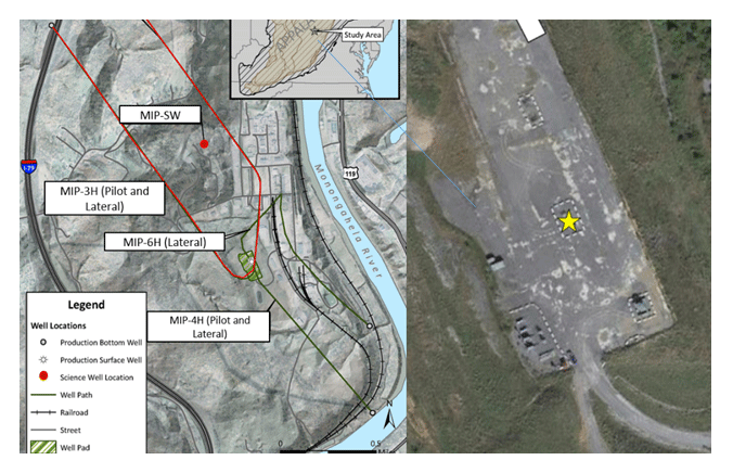
Figure 1 Location of the Marcellus Shale Energy and Environment Laboratory and the four production wells.

2.2 Air quality and meteorological data collection

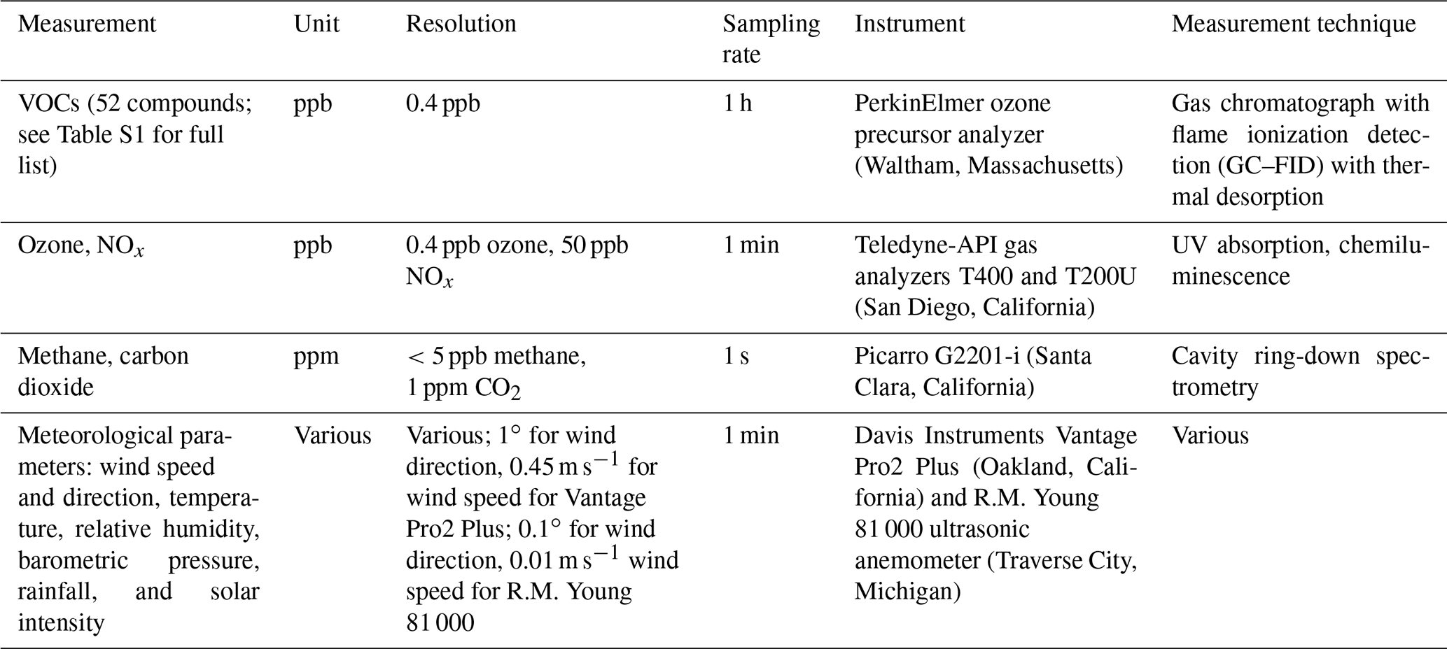
An ambient air monitoring laboratory (5.5 m trailer with ambient air sampled from inlets on the trailer roof) was situated at the northeastern corner of the MSEEL well pad (Fig. 1). With wind direction at this location most frequently from the southwest (Fig. 2), this position optimized the occurrences of the laboratory being downwind of the well pad. Instrumentation in the laboratory and measured constituents are listed in Table 1. All instruments were maintained and calibrated according to manufacturer's recommended protocols. Details of the laboratory assembly and operation have been previously described (Pekney et al., 2014).

Data collected at the air monitoring site are classified by activity at the well pad. Horizontal drilling occurred on 8 September–5 October 2015, first at well 5H then at well 3H. Hydraulic fracturing occurred on 10 October–16 November. Cleanout activities followed on 20–26 November, which involved using a diesel-powered coil tubing rig to drill out plugs and flush out residue left in the wells.

Flowback, the flowing of gas, formation fluid, and hydraulic fracturing fluid up the wells to the surface, took place over 10–14 December, after which both wells were in production. A reduced emission completion (REC) was performed; gas produced during this time was captured using portable equipment brought on site that separates the gas from the liquids so that the gas can be retained as a product.

Air monitoring began 18 September 2015 and ended 1 February 2016. No data were collected for the vertical drilling phase. Data collection was continuous except for calibration and instrument downtime. The laboratory's meteorological station measured relative humidity, temperature, rainfall, solar radiation, wind direction, wind speed, and barometric pressure at an elevation of 10 m.

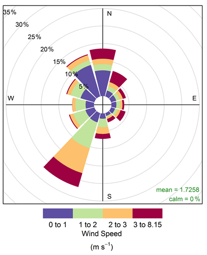
Figure 2 Wind speed and direction during the ambient air monitoring campaign at MSEEL (September 2015–February 2016).

Table 1 Constituents measured by the MSEEL mobile air monitoring laboratory (Pekney et al., 2018).

2.3 Source–receptor modeling

Positive matrix factorization (PMF), a factor analysis method (Fig. S7), was applied to hourly averaged ambient concentrations of measured species to identify possible sources and patterns for the stages of development. PMF decomposes the sample data into two matrices: factor profiles (representative of sources) and factor contributions (Brown et al., 2015; Norris et al., 2014). The fundamental objective of PMF is to solve the chemical mass balance (Eq. 1) between measured species concentrations and source profiles while optimizing goodness of fit (Eq. 2).

Mass balance is as follows (Evans and Jeong, 2007):

$$\begin{array}{}\text{(1)}& x_{i,j}=\sum _{k=\mathrm{1}}^p{g}_{ik}{f}_{kj}+e_{ij},\end{array}$$

where x_i,j is the data matrix with dimensions of i (observations) by j (chemical species), p is the optimal number of factors, g_ik is the factor contribution to the observation, f_kj is the species profile of the factor, k is the factor, and e_i,j is the residual concentration for each observation.

Goodness of fit is as follows:

$$\begin{array}{}\text{(2)}& Q={\sum }_{i=\mathrm{1}}^n{\sum }_{j=\mathrm{1}}^m{\left({\displaystyle \frac{x_{ij}-{\sum }_{k=\mathrm{1}}^p{g}_{ik}{f}_{ij}}{s_{ij}}}\right)}^{\mathrm{2}},\end{array}$$

where Q is the goodness of fit, n is the total number of observations, m is the total number of chemical species, and s_ij is the uncertainty for each observation. Summary of methods for uncertainty calculations are provided in the Supplement. Missing values within the dataset are replaced with the median value of that species; also, uncertainty for missing values is set at 4 times the species-specific median by the program. Multiple runs with different numbers of factors are executed for each dataset. The output of the PMF analysis needs to be interpreted by the user to identify the number of factors that may be contributing to the samples and the possible sources they represent. One of the main strengths of PMF analysis is that each sample is weighted individually, which allows the user to adjust the influence of each sample based on the measurement confidence.

Signal-to-noise ratio ($S/N$), an indicator of the accuracy of the variability in the measurements, can be used to identify a species as “strong”, “weak”, or “bad”. Generally, if this ratio is greater than 0.5 but less than 1, that species has a “weak” signal. “Strong” is the default value for all species with an assumption of $S/N$ greater than 1. The “bad” category excludes the species from the rest of the analysis. We considered the number of samples that are missing or below the detection limit when choosing the category for each species. (Norris et al., 2014). The expected goodness of fit (Q_expected) is calculated for each scenario (Norris et al., 2014).

Expected goodness of fit is as follows:

$$\begin{array}{}\text{(3)}& Q_{\text{expected}}=\left(i\times j\right)-\left\{\left(p\times i\right)+\left(p\times j\right)\right\},\end{array}$$

where (i×j) is the number of non-weak data values in X_ij, and (p×i) and (p×j) are the number of elements in G and F, respectively. Q_robust is the calculated goodness-of-fit parameter that excludes points that are not fit by the model. The lowest $Q_{\text{robust}}/Q_{\text{expected}}$ is calculated to compare different factor scenarios; when changes in Q become small with increasing factors, it can indicate that there may be too many factors in the solution (Brown et al., 2015).

In addition to these calculated parameters, factor profiles and error estimation diagnostics are used to compare the output of different simulations. Marker species (chemical species that are unique to a particular source) and temporal or seasonal variations can be used to aid in identifying the possible emission sources (Fig. 3). Associations between factors can also provide useful information for profile characterization. Moreover, meteorological data can provide useful information about the geographic location of the sources.

In order to perform the PMF analysis, we utilized a user-friendly graphical user interface (GUI) developed by the U.S. Environmental Protection Agency (EPA), EPA PMF 5.0 (Norris et al., 2014). Hourly average data were used for each pollutant to unify the measurement intervals. All pollutants included in the matrix were identified as “strong” (signal-to-noise ratio: $S/N$ >2). A total of 50 base runs were performed, and the run with the minimum Q value was selected as the base run solution. In each case, the model was run in the robust mode with a number of repeat runs to ensure the model least-squares solution represents a global rather than a local minimum. First, the rotational (linear transformation) F_peak variable was held at the default value of 0.0. However, there can be almost infinite possibilities of F and G matrices that produce the same minimum Q value, but the goal is producing a unique solution. As a result, rotational freedom is one of the main sources of uncertainty in PMF solutions (Paatero et al., 2014). Therefore, F_peak values were adjusted (−1.0, −0.5, 0.5, and 1.0) to explore how much rotational ambiguity exists in PMF solutions. In other words, the model adds and/or subtracts rows and columns of F and G matrices based on the F_peak, which is typically between −5 and +5 (Norris et al., 2014). Positive F_peak values cause a sharpened F matrix and smeared G matrix; negative F_peak values result in subtractions in the G matrix. The factor contributions were analyzed to find the optimum F_peak value.

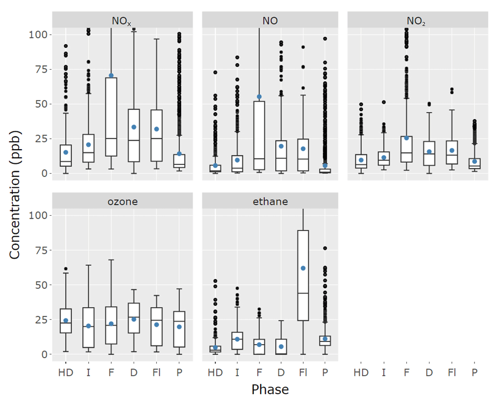
Figure 3 Summary statistics of input parameters for (a) NO_x, (b) NO, (c) NO₂, (d) ozone, and (e) ethane (HD: horizontal drilling; I: idle; F: fracturing; D: drillout; Fl: flowback; P: production). The idle phase consists of gaps of time between other operational phases, when there was little to no emissions-generating activity on the well pad.

The PMF analysis was completed with error estimation. We used three methods of error estimation: bootstrap (BS), displacement (DISP), and BS–DISP, which guide understanding the stability of the PMF solution (Norris et al., 2014). BS analysis is used to determine whether a set of observations affect the solution disproportionately. The main idea of BS analysis is to resample different versions of the original dataset and perform PMF analysis. Random errors and rotational ambiguity affect BS error intervals. The main reason for rotational ambiguity is the existence of infinite solutions similar to the solution generated by PMF solution. DISP analysis helps to analyze the PMF solution in detail. Only rotational ambiguity affects DISP error intervals.

BS–DISP is a hybrid method that gives more robust results than DISP results.

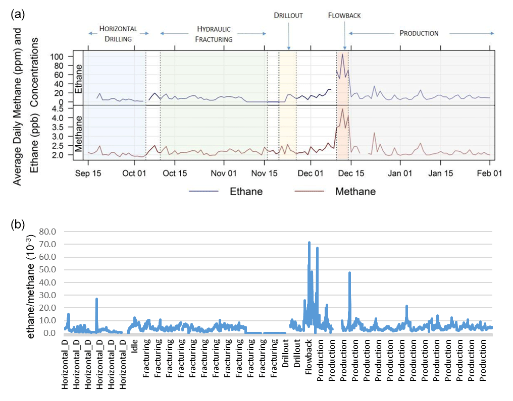
Figure 4 (a) Ethane and methane 24 h average concentrations and (b) the ratio of ethane to methane from drilling through the production monitoring period of well pad activity.

3 Results and discussion

3.1 Overview of results for measured compounds

Figure 3 shows a box-and-whisker graph of the measured NO_x, NO, NO₂, ozone, and ethane during the whole monitoring campaign at the study site. Similarly, Fig. 5 shows a statistical summary of methane and carbon dioxide. The y axis represents concentrations and the x axis represents the phases of the well development. The black line on each of the boxes represents the median for that particular dataset. The small circles represent outliers. The blue circles represent the mean. Since most of the VOC concentrations measured were consistently below 10 ppb, only ethane is included. There was an increase in NO_x (25th percentile (q1)=12.5 ppb) and NO (q1=2.7 ppb) during the fracturing phase compared to other phases. The whiskers show the high variability for this phase, which can be a result of small sample size for the fracturing phase. The $\mathrm{NO}/{\mathrm{NO}}_{\mathrm{2}}$ ratio for 25th and 75th percentiles was 1.2, indicating fresher, less oxidized emissions. The skewness of the data for this phase indicates that the data may not be normally distributed. The NO₂ graph shows a similar trend for the fracturing phase. We did not observe significant differences for different development phases for ozone, which is not surprising as it is a secondary pollutant and it can be related to the winter season of the data collection period (Edwards et al., 2014). There was a dramatic increase in ethane concentration for the flowback phase. This 25th percentile was 24 ppb, while this concentration ranged between 0 and 11 ppb for other phases. The 75th percentile was 89 ppb, which is a significantly higher value compared to other phases. We observed a similar trend for methane concentration. The 25th percentile (2.5 ppm) and the 75th percentile (4.3 ppm) were significantly higher than other phases. Differences for development phases for CO₂ were not statistically significantly different. CO₂ has many emissions sources and variable background concentrations, so distinguishing emissions from the well pad activities is difficult.

Figure 5 Summary statistics of input parameters for methane (a) and carbon dioxide for (b) HD, horizontal drilling; I, idle; F, fracturing; D, drillout; Fl, flowback; and P, production.

The average concentrations of methane and ethane for the entire monitoring campaign are shown in Fig. 4a. The highest ethane concentrations occurred during the flowback stage (565.7 ppb). A mean that is significantly higher than the median comes from a distribution that is skewed due to peak events (mean_ethane=11.4 ppb, median_ethane=8.5 ppb). Figure 4b shows the time series of ethane-to-methane ratios throughout the operational phases. The lowest average ratio occurred at horizontal drilling with 2.5, while the highest ratio occurred at the flowback phase with an average ratio of 17.4. The average ethane $/$ methane ratios for fracturing, drillout, and production phases are 3.4, 3.2, and 5.1, respectively.

The hourly concentration graphs of NO_x, O₃, CH₄, and CO₂ were used to analyze the factor solutions (Fig. S8). Hecobian et al. (2019) investigated the emissions during different well pad development phases to analyze emission rates in the Denver-Julesburg and Piceance basins in Colorado, US. They observed that emission rates of benzene and most VOCs were highest during flowback for both basins; on the other hand, they had much lower emission rates from the production phase, which can be related to the differences in duration of each phase (days to weeks). Light alkanes and benzene concentrations were higher during hydraulic fracturing. It is difficult to directly compare the results of the two studies, because the proposed study is based on continuous data during each phase while Hecobian et al. (2019) collected 374 measurements from five drilling, eight fracking, nine flowback, one liquid load out, and 11 production sites to analyze emission rate.

Figure S4 shows the dominant wind directions on overall concentrations, as well as giving information on the different concentration levels. Pollution roses show which wind directions contribute most to overall mean concentrations. For all air quality species, southwestern winds control the overall mean concentrations at the well pad. To explore the relationship between methane and ethane, we conditioned ethane by methane. Figure S5 indicates that higher ethane concentrations are associated with the SW and higher methane concentrations. The results also show that lower ethane and methane concentrations contributed from the east; the highest methane concentrations were obscured by a relatively high ethane background. The highest contribution to the factors was provided by the SW data (Fig. S6).

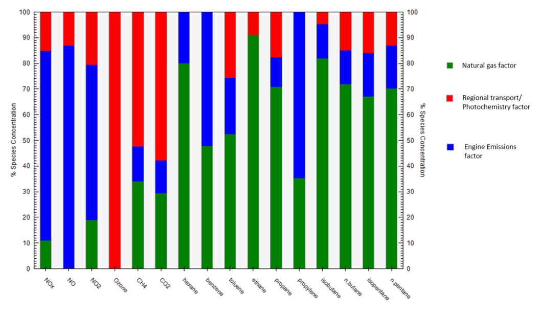
Figure 6 The three-factor solution fingerprints for drilling through the production monitoring period, F_peak=1.

3.2 Factor profiles

The three-factor model was chosen for the PMF analysis based on the interpretation of the factor profiles, Q_robust $/$ Q_expected ratios (Table S3), factor contributions, error estimation results (Table S4, Fig. S9), and hourly peak concentrations of pollutants. The three-factor solution was resolved to the following factors: natural gas for the natural-gas-related emissions sources, regional transport/photochemistry for the atmospheric regional molecular transport and oxidized background air, and engine emissions for emissions from vehicles, drill rigs, generators, and pumps used at the site (Fig. 5). The summary of PMF models with various peak values for well development activities are shown in Table S4. The DISP, BS, and BS–DISP results for two-, three-, and four-factor PMF solutions are summarized in Table S2. For the three-factor analysis, the DISP results indicate that there are no swaps and the PMF solution is stable, which means there are no exchange factor identities and it is a well-defined solution for the case. According to BS results, there is a small uncertainty; this could be an impact of high variability in concentration. BS–DISP captures both random errors and rotational ambiguity; these results also indicate that the solution is reliable because there are no swaps between factors for the PMF model. Error estimation summary plots (Fig. S9) show a range of concentration by species in each factor: base value, BS 5th, BS median, BS 95th, BS–DISP 5th, BS–DISP average, BS–DISP 95th, DISP min, DISP average, and DISP max.

3.3 Source profiles

The natural gas factor was named as such due to its composition of species that are present in natural gas: 89 % CO₂, 1 % methane, 3 % ethane, 1.5 % propane, 0.5 % isobutane, 1 % n-butane, 0.1 % pentane, and 0.2 % isopentane (Fig. S10). Ethane is a particularly good marker for natural gas emissions sources because its atmospheric sources are almost exclusively from natural gas extraction, production, processing, and use (Liao et al., 2017). A total of 92 % of ethane mass is explained by the natural gas factor (Fig. 6). The highest contribution for this factor occurred during the flowback phase.

The regional transport/photochemistry factor was characterized by high contributions from ozone (12 %), methane (1 %), and CO₂ (86 %) (Fig. S10). A total of 99 % of the ozone mass was explained by this factor (Fig. 6). Ozone is a product of photochemistry and not directly emitted by any of the sources on the well pad. Although CH₄ and CO₂ would be emitted by well pad sources, they are also present in background ambient air and could be transported to the monitoring location from other sources in the region. Contributions of this factor were relatively steady for all phases of operation during the entire monitoring campaign.

The engine emissions factor was composed of 39 % NO_x, 33 % NO, and 11 % NO₂ as well as 0.02 % toluene and 0.04 % benzene (Fig. S10). The portions of the mass of these species explained by this factor are 74 %, 87 %, 60 %, 20 %, and 54 %, respectively (Fig. 6). Toluene is released mainly from motor vehicle emissions and chemical spills (Gierczak et al., 2017). Another important emission source is oil and gas extraction (EPA, 1993). Contribution of this factor was significantly highest during hydraulic fracturing, when there were emissions from many diesel engines operating continuously on the well pad. Contribution during flowback was also elevated. Several peaks of contribution were observed during production, which could be due to maintenance vehicles and other short-lived vehicle-based activities on the well pad.

The main limitation of the study is having an uneven number of data points for each operational phase. This limitation affects the analyses; however, we do not have control of the durations of the operational phases. PMF models have several limitations. First, they need large datasets. In this study, the number of data varies based on the duration of the activity (Fig. S2). Therefore, the contribution to the factors is not the same for each phase. This is the main reason behind the uncertainty of defined factors. Second, the accuracy and precision of measured species limit the analysis. The determination of the number and character of factors is based on an expert's interpretation. Comprehensive information is needed on source profiles to verify the defined source profiles. Finally, the pre-set parameters play an important role in the model results. For future work, integrating more data from different fields can decrease the inherent uncertainty.

4 Conclusions

We investigated the effect of unconventional natural gas development activities on local air quality by using an ambient air monitoring laboratory near the Marcellus Shale well pad in Morgantown, West Virginia. The results of PMF solutions for well pad development phases show that there were three potential factor profiles as outlined in Fig. 5: natural gas, regional transport/photochemistry, and engine emissions. The horizontal drilling stage had an important contribution to the natural gas factor. In addition, there was a significant concentration contribution at the end of the horizontal drilling phase. An increasing contribution to engine emission factor was observed over different well pad drilling periods through production phases. The peak concentration was observed during the drillout stage. Even though it is difficult to compare the regional transport/photochemistry contributions due to high variability, the highest contributions occurred during horizontal drilling and drillout.

As determined by the PMF analysis, a measurable increase in natural-gas-related pollutant concentrations and the associated natural gas factor contribution from different stages of active phase was not observed. At the downwind distance of 600 m from the well pad center to the air monitoring laboratory, the emissions from the well pad were not easily distinguishable from typical variations in ambient background concentrations. West Virginia has many natural gas wells that contribute to the ambient background, as evidenced by ethane concentrations that are higher than the typical global background (Rinsland et al., 1987; Rudolph et al., 1996). Short-lived peak events that were observed when the wind direction was coming from the well pad show that emissions can be dispersed downwind and detected at this distance, but when concentrations are averaged and analyzed with a PMF analysis, the peak events were not significant enough to result in a measurable impact of the well pad emissions at the receptor location. Understanding the air quality impacts of operational phases is important since it has the potential to help inform future decision making and constrain cumulative impact assessments.