the Creative Commons Attribution 4.0 License.
the Creative Commons Attribution 4.0 License.
 | 26 Mar 2021
Technical note: On comparing greenhouse gas emission metrics
Nathan Clisby
Many metrics for comparing greenhouse gas emissions can be expressed as an instantaneous global warming potential multiplied by the ratio of airborne fractions calculated in various ways. The forcing equivalent index (FEI) provides a specification for equal radiative forcing at all times at the expense of generally precluding point-by-point equivalence over time. The FEI can be expressed in terms of asymptotic airborne fractions for exponentially growing emissions. This provides a reference against which other metrics can be compared.
Four other equivalence metrics are evaluated in terms of how closely they match the timescale dependence of FEI, with methane referenced to carbon dioxide used as an example. The 100-year global warming potential overestimates the long-term role of methane, while metrics based on rates of change overestimate the short-term contribution. A recently proposed metric based on differences between methane emissions 20 years apart provides a good compromise. Analysis of the timescale dependence of metrics expressed as Laplace transforms leads to an alternative metric that gives closer agreement with FEI at the expense of considering methane over longer time periods.
The short-term behaviour, which is important when metrics are used for emissions trading, is illustrated with simple examples for the four metrics.
- Article
(777 KB) - Full-text XML
- BibTeX
- EndNote


Anthropogenic contributions to global climate change come from a range of greenhouse gases. Comparisons between them have been facilitated by defining emission equivalence relations (which we denote by ≡), usually using CO2 as a reference.
The climatic influence of greenhouse gases is commonly represented in terms of radiative forcing, F, expressed in terms of MX, the atmospheric mass of gas X, with the effect of small perturbations linearised as
where aX is the radiative efficiency in mass units, i.e. the amount of change in radiative forcing per unit mass increase for constituent X in the atmosphere (Myhre et al., 2013).
Equivalence relations between sources of greenhouse gases are complicated because various gases are lost from the atmosphere on a range of different timescales. This behaviour is often represented using linear response functions, where the response function, RX(t), represents the proportion of ΔSX, the perturbation in emissions of constituent X, that remains in the atmosphere after time t. Thus the mass perturbation, ΔMX, is given as a convolution integral:
The outline of this note is as follows. In Sect. 2 we show how the prescription by Wigley (1998), which gives exact equivalence in radiative forcing between different time histories of emissions, may be elegantly expressed in terms of Laplace transforms. In Sect. 3, we adapt this representation to other metrics of emission equivalence and use it as inspiration for a new metric with a single adjustable parameter that accurately approximates equivalence in radiative forcing over timescales from decades to multiple centuries. In Sect. 4, we compare the different metrics in the time domain, and Sect. 5 discusses some of the mathematical characteristics that may bear on the political acceptance of alternative specifications of emission equivalence. We conclude in Sect. 6. Appendix A expresses the metrics in terms of frequency response, and Appendix B lists the notation. Enting and Clisby (2021) references the archived R code used in this paper.
Wigley (1998) defined an equivalence between emission histories, termed the FEI. Two emission histories are FEI equivalent if they lead to equivalent forcing at all times. In most cases, this requirement precludes point-by-point emission equivalence at all times.
Equivalent radiative forcing over all time from perturbations ΔSX and ΔSY in the emissions of gases X and Y requires
as the condition for
Subject to the conditions of linearity, this equivalence defines the exact equality of radiative forcing. However, it is an equivalence for emission profiles and not for instantaneous values.
A special case of FEI equivalence (see, for example, Enting, 2018) is when ΔSX and ΔSY both grow exponentially, with growth rate α and amplitudes cX and cY at t=0. Exponential growth has
The integral on the right is , the Laplace transform of RX(t), evaluated at p=α. Thus, for FEI equivalence of emissions growing exponentially at rate α one has
Interpreting these relations in terms of Laplace transforms can help clarify the different forms of equivalence metrics in the general case. More generally, for arbitrary emission perturbations the condition for FEI equivalence is defined by the Laplace transform of Eq. (3):
giving
In this expression is the Laplace transform of an integro-differential operator that acts on ΔSY(t) in the time domain. Differentiation of Eq. (5) shows that, for exponentially growing emissions, the asymptotic airborne fraction of a gas X is (e.g. Enting, 1990), and thus the FEI curve can be defined as the ratio of asymptotic airborne fractions for growth rate p.
The plot in Fig. 1 describes the specific case of methane, CH4, referenced to carbon dioxide, CO2. The solid line, denoted as FEI, can be interpreted in several different but mathematically equivalent ways:
-
it is the ratio of asymptotic airborne fractions for exponential growth, shown as a function of growth rate;
-
it gives the ratio that leads to FEI equivalence in the special case of exponentially growing emissions;
-
it is the Laplace transform of an operator ΨFEI that acts on methane emission functions to produce FEI-equivalent CO2 emissions.
In these last two cases, the FEI equivalence is achieved by scaling by .
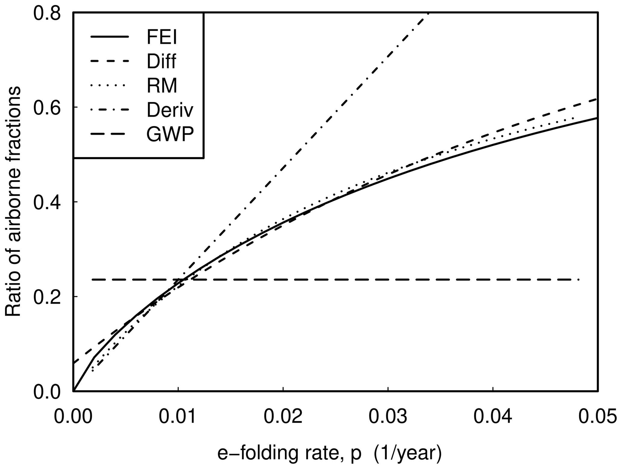
Figure 1Ratio of airborne fractions for CH4 relative to CO2 as defined or assumed for various metrics. The solid curve shows the forcing equivalent index (FEI), which acts as a reference. The global warming potential (GWP) treats this ratio as independent of timescale (Eq. 16); the chain line for the “Deriv” case treats the timescale dependence as proportional to the inverse timescale (Eq. 19); the shorter dashes of the “Diff” curve (Eq. 21) more closely approximate FEI. The dotted line is an empirical reduced model (RM) approximation (Eq. 23) to FEI. These curves can also be interpreted as the Laplace transforms of the operations that define the equivalence in the time domain.
The examples given here compare four different metrics, again for the case of CH4 referenced to CO2, benchmarking them against FEI. A general linear, time-invariant equivalence relation can be defined by
In the time domain, such a metric can be regarded as a process that extracts, from the history of CH4 emissions, an index or statistic that gives CO2 equivalence. Such a metric can be assessed in radiative forcing terms by the accuracy of the approximation
If the global temperature response to a change in radiative forcing is linearised using a response function U(t), as is done, for example, by Myhre et al. (2013), then equivalence in temperature perturbations can be analysed in terms of
In both Eqs. (10) and (11), removing the common factors reduces the comparison to one of considering the accuracy of the approximation
As Wigley (1998) noted, “if CO2 equivalence is based on radiative forcing and calculated accurately for non-CO2 gases, then the temperature and sea-level implications of the [Kyoto] Protocol may be calculated from the CO2-alone case”.
Because of the commutative and associative properties of such transformations, a transformation of the CH4 source to give an equivalent CO2 source can be described in terms of how well the metric transformation, acting on the CO2 impulse response, reproduces the impulse response for CH4. The application of this relation in the frequency domain (i.e. p=2πif) is described in Appendix A.
In these calculations, the response used for CO2 is the multi-model mean from Joos et al. (2013, their Table 5) and the response of CH4 described by a 12.4-year perturbation lifetime (Myhre et al., 2013). In each case, these represent the response to small perturbations from of current conditions, reflecting our interest in the use of metrics for trade-offs, reporting and target-setting. The values for and are also taken from (Myhre et al., 2013), and in the latter case follow the IPCC convention of including indirect effects. These factors only appear in the relative scaling of the axes in the two parts of Fig. 2.
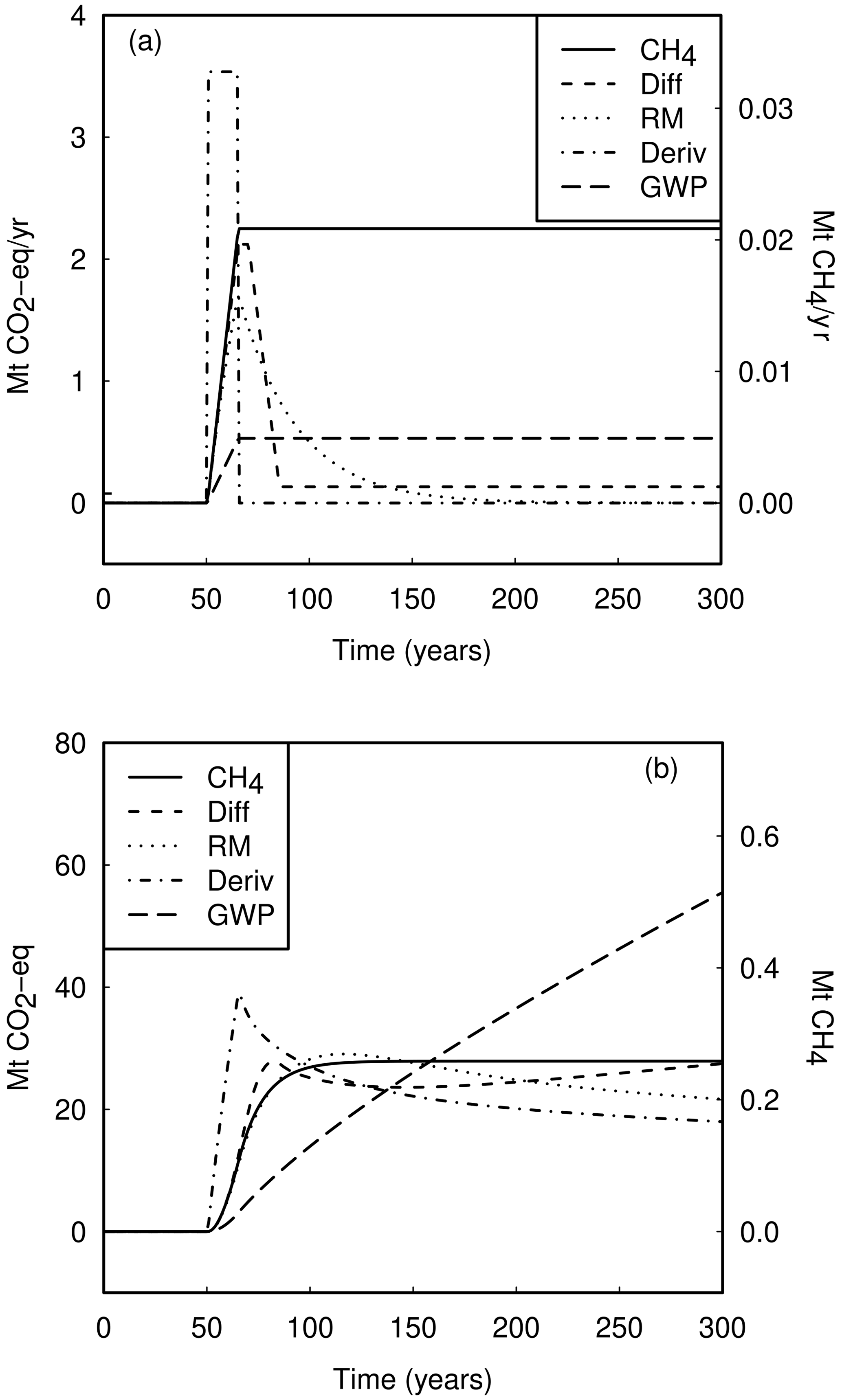
Figure 2(a) A CH4 source representing an increase over 15 years from zero to a constant (solid line) and the CO2-equivalent sources as defined by the various metrics described in Sect. 3. The relative scaling of the CH4 and CO2 axes is . (b) CH4 concentrations from the source shown in panel (a) (solid line) and the CO2 concentrations resulting from the CO2 concentrations resulting from the equivalent CO2 sources, as shown in panel (a). The relative scaling of the axes is so that the radiative forcing can be compared directly.
The calculations were developed for methane emissions from active biological sources. For fossil methane, an additional CO2 contribution from the oxidation of CH4, corresponding to a global warming potential (GWP) of 1, should be included.
3.1 Global warming potential
The GWP with time horizon H defines an equivalence (denoted ) for component Y given by
where
Although Eq. (14) is usually written without the H−1 factors, in the form above the numerator and denominator correspond to the airborne fractions of Y and CO2, respectively, averaged over the time horizon H and multiplied by the factor , which corresponds to 𝖦𝖶𝖯0, the H→0 limit of 𝖦𝖶𝖯H. This factor can be called the instantaneous GWP.
𝖦𝖶𝖯100, the GWP with the time horizon H=100 years, has become the standard for greenhouse gas equivalence in international agreements.
For CH4, the equivalence is
where all use of GWP in what follows will specifically refer to CH4. Relation (15) corresponds to using
which is plotted as the horizontal line (long dashes) in Fig. 1.
However, this definition of equivalence has long been known to be poor (e.g. Wigley, 1998; Reilly et al., 1999), especially for emission profiles approaching stabilisation of concentrations.
For H>100 the approximation
is quite close (Enting, 2018). Thus, in the context of emissions growing with e-folding time, H, 𝖦𝖶𝖯H gives approximate FEI equivalence. Specifically, 𝖦𝖶𝖯100 gives approximate equivalence for 1 % a−1 growth rate and, as shown in Fig. 1, about a 30 % underestimate for the 2 % a−1 growth rate that approximately characterises 20th-century changes.
3.2 Derivative
Several studies (Smith et al., 2012; Lauder et al., 2013) suggested that for short-lived gases such as CH4, changes in emissions in the short-lived gases should be related to one-off CO2 emissions. This suggests a metric of the following form:
or (as a Laplace transform)
which is plotted as the straight line through the origin (chain curve) in Fig. 1.
Subsequently, the search for an improved metric, termed GWP*, has been the subject of extensive studies undertaken by Allen and co-workers (Allen et al., 2016, 2018; Jenkins et al., 2018; Cain et al., 2019; Collins et al., 2020; Lynch et al., 2020). These studies had included cases defined by linear combinations of the derivative metric and GWP. Such cases are not shown in the transform domain illustrated in Fig. 1 but correspond to linear functions of p that do not pass through the origin.
3.3 Difference
A recent proposal for an improved GWP* (Cain et al., 2019) defined the equivalence as follows:
The Laplace transform is derived using the generic result that a time shift by T corresponds to multiplying the Laplace transform by exp (−pT), giving
This is shown in Fig. 1 using the short dashes.
3.4 Reduced model
When the response functions are expressed as sums of exponentially decaying functions of time as is done here, the Laplace transforms become a sum of partial fractions of the form , and thus the combinations of response functions will be ratios of polynomials in p. Thus, the FEI ratio will also be a ratio of polynomials that can in turn be re-expressed as a sum of partial fractions. Formally, this gives an exact form for the FEI relation, but it is one which would have perhaps 6 to 10 parameters and be too complicated for practical use. Studies in a number of fields, such as electronic engineering (e.g. Feldman and Freund, 1995), have noted that such expressions can often be usefully approximated by lower-order expressions. For emission equivalence, it is only practical to use very low-order approximations for such a reduced model.
As shown in Fig. 1, a close fit to FEI can be obtained with the reduced model (RM) given by
with b=0.035, which is plotted as the dotted curve in Fig. 1.
This gives the following equivalence:
In the time domain, Eq. (23) becomes
where denotes the rate of change in the perturbation to CH4 emissions.
This expresses the CO2 equivalent of CH4 as a weighted average of the CH4 emission growth rate. Consequently, the metric retains the property that constant emissions of CH4 are treated as equivalent to zero CO2 emissions as in derivative metrics (Smith et al., 2012; Lauder et al., 2013). The parameter b can be chosen to match other metrics. The value b=0.035 is chosen so that for emissions with 1 % a−1 growth rate the RM metric closely matches the 100-year GWP.
For specific calculations it may be more appropriate to represent this metric as
Relation (25) is derived from Eq. (24) using integration by parts (or equivalently by putting ). It has the advantage that it is expressed in terms of emissions rather than their rates of change.
Equation (25) defines the reduced model equivalence as a difference between present emissions and a weighted average of past emissions. When considered in terms of frequency f (by setting ) this avoids the frequency aliasing that occurs with the difference metric for periods of 20 years or integer fractions thereof (see Fig. A1 which is described in Appendix A).
The equivalence relation (23) can also be re-written as
This defines an equivalence between the rate of change of CH4 emissions and a combination of rate of change of CO2 emissions (as in GWP) and current CO2 emissions (as in the derivative-based equivalences suggested by Smith et al., 2012 and Lauder et al., 2013).
Many previous studies of metrics have concentrated on global-scale calculations over the long term. As discussed above, this has led to the development of metrics based on rates of change. However, as discussed in Sect. 5 below, for emissions trading on shorter timescales, political acceptance is likely to favour metrics that also have equivalent influences in the short term. The short-term behaviour can be analysed by taking a notional CH4 emission profile and calculating the resulting CH4 concentrations. This is then compared to the CO2 concentrations that result from the notionally equivalent CO2 emissions.
Figure 2a shows a CH4 source perturbation with a rapid increase from zero to a fixed emission rate, and the CO2-equivalent emissions as determined by the various equivalence metrics. Figure 2b shows the CH4 concentration resulting from the methane emissions and the CO2 concentration resulting from the various CO2-equivalent emissions. In Fig. 2a and b, the relative scaling of the axes is given by so that forcing can be compared directly. In this scaling, the direct effect of CH4 has been scaled to include indirect effects, from tropospheric ozone and stratospheric water vapour, using values taken from Myhre et al. (2013). Note that the indirect effects are not included in the corresponding graphs given by Enting and Clisby (2020).
The results in Fig. 2b clearly show the failings of the 100-year GWP for defining emission equivalence for constant sources. The forcing from GWP-equivalent CO2 (long dashes) initially lags well behind the actual forcing from CH4 but in the long term it continues to increase indefinitely long after the forcing from on-going CH4 emissions has stabilised. Compared to this behaviour, the derivative metric based on rates of change of CH4 emissions is a great improvement (chain curve). However, the CO2-equivalent forcing initially exceeds the actual forcing from CH4 and in the long-term drops below the CH4 forcing. The difference metric from Cain et al. (2019) (short dashes) provides a CO2-equivalent forcing that follows the actual CH4 forcing more closely with only a slight shortfall in the longer term. After t=150 the forcing from equivalence defined by the Cain et al. (2019) metric (short dashes) starts to increase, due to the contribution that corresponds to 0.25 times GWP when .
Figure 2b shows that the CO2-equivalence derived from the reduced model (dotted curve) follows the actual CH4 forcing particularly closely, as would be expected given the close agreement when the relations are expressed as Laplace transforms as shown in Fig. 1.
The nature of the FEI relation precludes close matches in forcing from instantaneous relations between CH4 and CO2 emissions. The difference and reduced model metrics relate CO2 equivalents to the past history of CH4 emissions. For a specific case, Lauder et al. (2013) suggested an approximate equivalence to step changes in methane emissions balanced by an ongoing future CO2 uptake from growing trees.
The aim of our analysis has been to provide a better understanding GWP vs. GWP* and similar metrics. Any comprehensive analysis of what might be politically feasible needs to be done by others with greater expertise in such areas. However, there are various aspects of our analysis that bear on the practical applicability and political acceptability of various metrics and the trade-offs that need to be balanced in political choices.
Past studies cited above suggest that an equivalence metric should capture the context of emissions at the time. The analysis by Enting (2018) (see also Eq. 17 above) notes that 𝖦𝖶𝖯H is close to FEI equivalence for growth in emissions with an e-folding time of H. Thus, a 100-year GWP was a plausible approximation at the time that it was introduced. For very large H, the GWP of short-lived gases goes to zero as , suggesting that a derivative of growth rates should define the metric for such long timescales. In contrast, for short-term trading and target setting, a metric that captures the short-term context is desirable in order to avoid distortions that would hinder political acceptability.
An important goal of defining emissions equivalence is to allow for emissions of different greenhouse gases to be substituted for each other so that a given target expressed in terms of radiative forcing (or equivalently in terms of CO2 concentration equivalence) can be achieved for the lowest economic cost. If, as is the case for 𝖦𝖶𝖯100, the metric overestimates the extent to which CO2-equivalent emission reductions contribute to radiative forcing, then methane reductions based on such equivalence will fall short of the CO2 concentration-equivalent target. Conversely, for short timescales where 𝖦𝖶𝖯100 underestimates the forcing reduction of CO2-equivalent methane reductions, short-term targets based on such equivalence will overestimate the extent of requisite methane emission reductions as in the example given by Wigley (1998).
In considering how our analysis feeds into such considerations, we make the following notes:
-
the metric should capture both the long-term context needed for stabilisation and the more immediate context in which both trading and international agreements are conducted;
-
if the metric for emissions equivalence is too complex, as it is for FEI, then it may be difficult or impossible for an effective trading scheme to be implemented;
-
the metric needs to be “backward looking” and avoid giving present credit or debit on the basis of promises of future targets;
-
the backwards view should not extend too far, as the relevant actors can change over time, even in the cases of nations or multi-national groups, such as the EU, which has in the past set collective targets;
-
metrics defined in terms of derivatives need to be supplemented with a specification of how this is determined in practice, e.g. as a difference by Cain et al. (2019) or the transformation from Eq. (24) in terms of rates of change of sources to Eq. (25) in terms of actual sources for the reduced model metric.
Finally, we note that our analysis is illustrative, using specific numbers primarily from the 5th IPCC assessment. The forthcoming 6th IPCC assessment may well make minor changes to specific numbers, such as the effective lifetime and the CO2 response function as well as things such as the inclusion of feedbacks, forcing efficiencies and indirect effects (cf. Myhre et al., 2013).
Our analysis has used the concept of FEI equivalence to analyse various definitions of greenhouse gas emission equivalence in terms of how closely equivalent emissions at a time t lead to equal radiative forcing at future times. The approach is applied to the consideration of CH4 emissions in terms of various definitions of their CO2-equivalent emissions. In the special case of exponentially growing emissions, FEI equivalence can be achieved when the emissions are scaled by the instantaneous (0 time horizon) GWP multiplied by the ratio of the asymptotic airborne fractions. This ratio depends on the e-folding growth rate. Various emission metrics can be compared in terms of how well they match this ratio at the range of relevant timescales. This analysis is equivalent to considering Laplace transforms of the impulse response functions of the respective gases.
GWP treats this ratio as a constant for all timescales, effectively defining 𝖦𝖶𝖯H as the instantaneous GWP multiplied by the ratio of average airborne fractions over the time horizon, H. For CH4, referenced to CO2, this means that 𝖦𝖶𝖯H overestimates the CH4 contribution for growth rates less than and underestimates the CH4 contribution to radiative forcing at faster growth rates.
Metrics relating CO2 equivalence to rates of change of CH4 emissions or emissions of other short-lived gases are treating the ratio of airborne fractions as proportional to the e-folding rate. This can provide a good representation of long-term behaviour relevant for stabilisation, but overestimates the role of CH4 on the shorter timescales relevant for emission trading. A range of metrics that better match FEI over a wide range of timescales from decades to millennia can be constructed. These include the metric proposed by Cain et al. (2019), which uses the change in CH4 emissions over a 20-year interval, and a reduced model approximation to FEI equivalence. In each of these cases the better match is achieved at the expense of comparisons involving longer time periods.
The political acceptability of metrics other than the GWP will involve various trade-offs between accuracy and practicality. The type of analyses presented here can help analyse such trade-offs without reference to specific scenarios of changes in greenhouse gas emissions.
The Laplace transform provides a natural formalism for analysing causal initial value systems. However, Fourier transforms and Fourier analyses have wide familiarity and can be used to describe our results.
For a periodic variation with exponentially increasing amplitude, Eq. (5) generalises to
For , this relation requires α>0 in order to have the lower limit of the left-hand integral and the upper limit of the right-hand integral defined. The α→0 limit shows the relation between the Laplace transform and the Fourier transform, which, for functions with R(t)=0 for t<0, is given by the integral on the right.
Section 3 noted that metric transformations defined by
can be assessed in radiative forcing terms by the accuracy of the approximation
which reduces to comparing
where for FEI equivalence the approximation becomes exact equality.
A frequency domain interpretation can be obtained by putting p=2πif. In these terms, the metric transformation is acting like a frequency equaliser in an audio system.
The phases of the complex numbers in the relations above capture the phase shifts for the various frequencies. For the present we show only the resulting amplitudes, given by the moduli, () of the complex value and ignore the phase (noting that the modulus of a product is the product of the moduli).
Figure A1 sets p=2iπf to evaluate the various cases considered in the paper, as functions of frequency f in cycles per year. It shows the following results:
-
, the “target” for FEI equivalence (the zero frequency value is the perturbation lifetime);
-
, i.e. a multiple of the CO2 response, growing indefinitely as frequency goes to zero;
-
, which gives a better approximation over a wider range of frequencies;
-
, which gives a further improvement but a notable discrepancy for cycles whose period is near the 20-year interval used in the difference calculation;
-
, which gives a still closer fit over the range of frequencies shown.
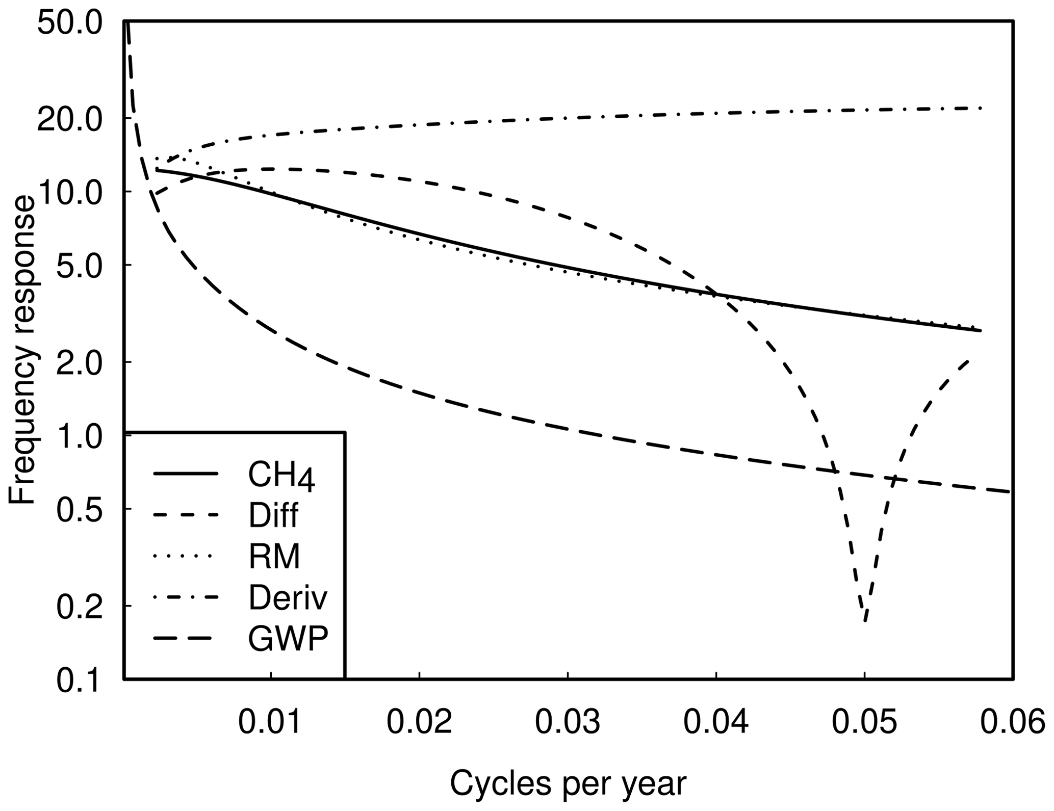
Figure A1Frequency response for the various cases of discussed above, compared to the actual frequency response, to periodic CH4 emissions (solid line), using p=2πif.
Laplace transforms are denoted by the tilde notation with as the Laplace transform of R(t).
Equivalence relations are denoted by ≡ with particular cases
identified, e.g. .
| aX | Radiative forcing per unit mass of constituent X. |
| b | e-folding rate in reduced model equivalence relation. |
| FX(t) | Radiative forcing of constituent X. |
| GWP, 𝖦𝖶𝖯H | Global warming potential for CH4 (unless otherwise specified), for time horizon H. |
| H | Time horizon for GWP. |
| MX(t) | Atmospheric mass of constituent X. Perturbation is ΔMX(t). |
| p | Argument of Laplace transform (equivalent to e-folding rate when comparing exponentially |
| growing emissions). | |
| RX(t) | Atmospheric response function for constituent X. |
| SX(t) | Anthropogenic emission of constituent X. Perturbation is ΔSX(t). |
| t | Time. |
| X,Y | Labels for constituent (CO2, CH4). |
| α | e-folding rate of exponentially growing emissions. |
| δ(t) | Delta “function” or instantaneous unit pulse, i.e. the notional derivative of unit step function. |
| Laplace transform of generic integro-differential operator that defines a metric transformation. | |
| (, , , and ). |
The R code used to perform the calculations and generate the figures is archived in FigShare at https://doi.org/10.6084/m9.figshare.13667657 (Enting and Clisby, 2021).
No data sets were used in this article.
IE and NC worked on the mathematical analysis, the computer code, and the writing and checking of the manuscript.
The authors declare that they have no conflict of interest.
The authors gratefully acknowledge the contribution of Alan Lauder in bringing the issue of CH4 vs. CO2 comparisons to our attention. We also wish to thank Annette Cowie for valuable comments on the manuscript. We also acknowledge helpful review comments from William Collins and the anonymous referee.
This paper was edited by Tim Butler and reviewed by William Collins and one anonymous referee.
Allen, M. R., Fugelstvedt, J. S., Shine, K. P., Reisinger, A., Pierrehumbert, R. T., and Forster, P. M.: New use of global warming potentials to compare cumulative and short-lived climate pollutants, Nat. Clim. Change, 6, 773–777, 2016. a
Allen, M. R., Shine, K. P., Fugelstvedt, J. S., Millar, R. A., Cain, M., Frame, D. J., and Macey, A. M.: A solution to the misrepresentation of CO2-equivalent emissions of short-lived climate pollutants under ambitious mitigation, npj: Climate and Atmospheric Science, 1, 16, https://doi.org/10.1038/s41612-018-0026-8, 2018. a
Cain, M., Lynch, J., Allen, M. R., Fugelstvedt, J. S., Frame, D. J., and Macey, A. M.: Improved calculation of warming-equivalent emissions for short-lived climate pollutants, npj: Climate and Atmospheric Science, 2, 29, https://doi.org/10.1038/s41612-019-0086-4, 2019. a, b, c, d, e, f
Collins, W., Frame, D. J., Fugelstvedt, J. S., and Shine, K. P.: Stable climate metrics for emissions of short- and long-lived species – combining steps and pulses, Environ. Res. Lett., 15, 024018, https://doi.org/10.1088/1748-9326/ab6039, 2020. a
Enting, I. G.: Ambiguities in the calibration of carbon cycle models, Inverse Probl., 6, L39–L46, 1990. a
Enting, I. G.: Metrics for greenhouse gas equivalence, in: Encyclopedia of the Anthropocene, edited by: Dellasala, D. A. and Goldstein, M. I., Elsevier, Oxford, UK and Waltham, MA, USA, 467–471, 2018. a, b, c
Enting, I. and Clisby, N.: Technical note: On comparing greenhouse gas emission metrics, Atmos. Chem. Phys. Discuss. [preprint], https://doi.org/10.5194/acp-2020-996, in review, 2020. a
Enting, I. G. and Clisby, N.: R code for ACP-2020-996. Technical note on comparing greenhouse gas emission metrics, FigShare, https://doi.org/10.6084/m9.figshare.13667657, 2021. a, b
Feldman, P. and Freund, R. W.: Efficient linear circuit analysis by Pade approximation via the Lanczos process, IEEE Trans Computer aided design of integrated circuits and systems, 14, 639–649, 1995. a
Jenkins, S., Millar, R. J., Leach, N., and Allen, M. R.: Framing climate goals in terms of cumulative CO2-forcing-equivalent emissions, Geophys. Res. Lett., 45, 2795–2804, https://doi.org/10.1002/2017GL076173, 2018. a
Joos, F., Roth, R., Fuglestvedt, J. S., Peters, G. P., Enting, I. G., von Bloh, W., Brovkin, V., Burke, E. J., Eby, M., Edwards, N. R., Friedrich, T., Frölicher, T. L., Halloran, P. R., Holden, P. B., Jones, C., Kleinen, T., Mackenzie, F. T., Matsumoto, K., Meinshausen, M., Plattner, G.-K., Reisinger, A., Segschneider, J., Shaffer, G., Steinacher, M., Strassmann, K., Tanaka, K., Timmermann, A., and Weaver, A. J.: Carbon dioxide and climate impulse response functions for the computation of greenhouse gas metrics: a multi-model analysis, Atmos. Chem. Phys., 13, 2793–2825, https://doi.org/10.5194/acp-13-2793-2013, 2013. a
Lauder, A. R., Enting, I. G., Carter, J. O., Clisby, N., Cowie, A. L., Henry, B. K., and Raupach, M.: Offsetting methane emissions – An alternative to emission equivalence metrics, Int. J. Greenh. Gas Con., 12, 419–429, 2013. a, b, c, d
Lynch, J., Cain, M., Pierrehumbert, R., and Allen, M.: Demonstrating GWP* as a means of reporting warming-equivalent emissions that captures the contrasting impacts of short- and long-lived climate pollutants, Environ. Res. Lett., 15, 044023, https://doi.org/10.1088/1748-9326/ab6d7e, 2020. a
Myhre, G., Shindell, D., Bréon, F.-M., Collins, W., Fuglestvedt, J., Huang, J., Koch, D., Lamarque, J.-F., Lee, D., Mendoza, B., Nakajima, T., Robock, A., Stephens, G., Takemura, T., and Zhang, H.: Anthropogenic and Natural Radiative Forcing, in: Climate Change 2013: The Physical Science Basis. Contribution of Working Group I to the Fifth Assessment Report of the Intergovernmental Panel on Climate Change, edited by: Stocker, T., Qin, D., Plattner, G.-K., Tignor, M., Allen, S., Boschung, J., Nauels, A., Xia, Y., Bex, V., and Midgley, P., Cambridge University Press, Cambridge, UK and New York, NY, USA, 2013. a, b, c, d, e, f
Reilly, J., Prinn, R., Harnisch, J., Fitzmaurice, J., Jacoby, H., Kicklighter, D., Melillo, J., Stone, P., Sokolov, A., and Wang, C.: Multi-gas assessment of the Kyoto Protocol, Nature, 401, 549–555, 1999. a
Smith, S. M., Lowe, J. A., Bowerman, N. H. A., Gohar, L. K., Huntingford, C., and Allen, M. R.: Equivalence of greenhouse-gas emissions for peak temperature limits, Nat. Clim. Change, 2, 535–538, 2012. a, b, c
Wigley, T. M. L.: The Kyoto Protocol: CO2, CH4 and climate implications, Geophys. Res. Lett., 25, 2285–2288, 1998. a, b, c, d, e
- Abstract
- Introduction
- Metrics: forcing equivalent index (FEI)
- Comparison of metrics
- Comparisons in the time domain
- Practical issues for implementation
- Concluding summary
- Appendix A: Frequency domain analysis
- Appendix B: Notation
- Code availability
- Data availability
- Author contributions
- Competing interests
- Acknowledgements
- Review statement
- References