Turbulence-permitting air pollution simulation for the Stuttgart metropolitan area

Air pollution is one of the major challenges in urban areas. It can have a major impact on human health and society and is currently a subject of several litigations in European courts. Information on the level of air pollution is based on near-surface measurements, which are often irregularly distributed along the main traffic roads and provide almost no information about the residential areas and office districts in the cities. To further enhance the process understanding and give scientific support to decision makers, we developed a prototype for an air quality forecasting system (AQFS) within the EU demonstration project “Open Forecast”.

For AQFS, the Weather Research and Forecasting model together with its coupled chemistry component (WRF-Chem) is applied for the Stuttgart metropolitan area in Germany. Three model domains from 1.25 km down to a turbulence-permitting resolution of 50 m were used, and a single-layer urban canopy model was active in all domains. As a demonstration case study, 21 January 2019 was selected, which was a heavily polluted day with observed PM₁₀ concentrations exceeding 50 µg m⁻³.

Our results show that the model is able to reasonably simulate the diurnal cycle of surface fluxes and 2 m temperatures as well as evolution of the stable and shallow boundary layer typically occurring in wintertime in Stuttgart. The simulated fields of particulates with a diameter of less than 10 µm (PM₁₀) and nitrogen dioxide (NO₂) allow a clear statement about the most heavily polluted areas apart from the irregularly distributed measurement sites. Together with information about the vertical distribution of PM₁₀ and NO₂ from the model, AQFS will serve as a valuable tool for air quality forecasting and has the potential of being applied to other cities around the world.

1 Introduction

Currently, more than 50 % of the global population lives in cities, whereas the United Nations (UN) expect a further increase by about 10 % in 2030 (UN, 2018). The UN also expects that in 2030 34 % of the world population will reside in cities with more than 500 000 inhabitants.

Due to a strong increase of road traffic in major European cities (Thunis et al., 2017), pollution limits are often violated in larger cities. For example, for particulate matter with particle diameters less than 10 µm (PM₁₀), the critical value is an annual mean concentration of 20 µg m⁻³ or a daily mean value of 50 µg m⁻³ (WHO, 2005). For nitrogen dioxide (NO₂), the critical values are 200 and 40 µg m⁻³ as daily and annual mean values, respectively.

The violation of these pollution limits can lead to health and environmental problems and is currently part of several litigations, e.g., at the German Federal Administrative Court dealing with possible driving bans for non-low-emission vehicles. The basis for these litigations are mostly a few local, unevenly distributed observations. In combination with special meteorological conditions like wintertime thermal inversion layers, it can be misleading to draw conclusions about the overall air quality in the city only from single observations. According to, e.g., the German Federal Immission Control Ordinance (https://www.gesetze-im-internet.de/bimschv_39/anlage_3.html, last access: 23 March 2021), it is sufficient that traffic-related measurements are representative of a section of 100 m, but this is not representative of the commercial and office districts in the cities that are suffering from traffic control in the case of fine dust alerts and residential areas. Namely in residential areas, health protection action plans require representative air quality measures.

Therefore, it becomes important to apply a more scientifically valid approach by applying coupled atmospheric and chemistry models to predict air quality. Regional and global atmospheric models like the Weather Research and Forecasting (WRF) model (Skamarock et al., 2019), the Consortium for Small Scale modeling (COSMO; Baldauf et al., 2011), the Icosahedral Nonhydrostatic model (ICON; Zängl et al., 2015), or the Regional Climate Model system (RegCM4; Giorgi et al., 2012) are often used to force offline chemistry transport models like CHIMERE (Mailler et al., 2017), LOng Term Ozone Simulation – EURopean Operational Smog (LOTOS-EUROS) (Manders et al., 2017), EURopean Air Pollution Dispersion (EURAD; Memmesheimer et al., 2004), and Model for OZone And Related chemical Tracers (MOZART) (Brasseur et al., 1998; Horowitz et al., 2003).

Several studies showed that combining an atmospheric model with an online coupled chemistry component is a suitable tool for air quality and pollution modeling in urban areas at the convection-permitting (CP) resolution (Fallmann et al., 2014; Kuik et al., 2016, 2018; Zhong et al., 2016; Huszar et al., 2020) .

Compared to chemical transport models, coupled models like the Weather Research and Forecasting model with its coupled chemistry component (WRF-Chem) (Grell et al., 2005), COSMO-ART (Vogel et al., 2009), ICON-ART (Rieger et al., 2015), and the Integrated Forecasting System (IFS) MOZART (Flemming et al., 2015) allow for a direct interaction of aerosols with radiation, leading to a better representation of the energy balance closure at the surface as would be the case when applying an offline chemistry model.

As the terrain and land cover over urban areas usually show fine-scale structures which are not resolved even by a CP resolution, there is a need for turbulence-permitting (TP) simulations with horizontal grid increments of a few hundred meters or even less. Important features are, e.g., urban heat island effects (Fallmann et al., 2014, 2016; García-Díez et al., 2016; Li et al., 2019) and local wind systems like mountain and valley winds due to differential heating (Corsmeier et al., 2011; e.g., Jin et al., 2016). Also, micro- and mesoscale wind systems can develop due to urban structures and the heterogeneity of the land surface. It is well known that TP simulations are a promising tool to further enhance the understanding of processes in the atmospheric boundary layer (Heinze et al., 2017a, b; Panosetti et al., 2016; Bauer et al., 2020) in urban areas (Nakayama et al., 2012; Maronga et al., 2019, 2020).

In order to further enhance the quality of the simulations, building and urban canopy models (UCMs) are developed (Martilli et al., 2002; Kusaka and Kimura, 2004; Salamanca and Martilli, 2010; Maronga et al., 2019; Scherer et al., 2019; Teixeira et al., 2019). The main purpose of UCMs is to provide a better description of the lower boundaries over urban areas such as building, roof, and road geometries and their interactions with atmospheric water vapor, wind, and radiation.

With the EU-funded “Open Forecast” project (https://open-forecast.eu/en/, last access: 23 March 2021), it was intended to develop a prototype for an air quality forecasting system (AQFS) for the Stuttgart metropolitan area in southwest Germany. Open Forecast is a demonstration project to show the potential of open data combined with supercomputer resources to create new data products for European citizens and public authorities. The long-term goal is to provide end users and political decision makers a useful tool, particularly considering further urbanization and heat island effects as well as potential driving restrictions due to recent EU decisions on emission limits.

For our AQFS, we use the WRF-Chem NWP model (Grell et al., 2005; Skamarock et al., 2019), as the WRF model is extensively evaluated over Europe at different timescales and horizontal resolutions (San José et al., 2013; Warrach-Sagi et al., 2013; Milovac et al., 2016; Lian et al., 2018; Molnár et al., 2019; Bauer et al., 2020; Coppola et al., 2020; Schwitalla et al., 2020). It can easily be set up in a nested configuration over all regions of the Earth. Compared to the Parallelized Large-Eddy Simulation Model (PALM) (Maronga et al., 2015) for urban applications (PALM-4U), the nested model domains are driven by the full atmospheric and chemical information from the parent domain along its lateral boundaries. Also, it contains well-characterized combinations of parameterizations of turbulence and cloud microphysics in the outer domain that are consistent with the inner TP domains where the high-quality cloud parameterization remains. No switch between different model systems is required, which is expected to provide a great advantage with respect to the skill of air pollution and meteorological forecasts.

To enhance the forecast skill, suitable variational and ensemble-based data assimilation systems are already in place to further improve the meteorological initial conditions (Barker et al., 2012; Zhang et al., 2014; Kawabata et al., 2018; Thundathil et al., 2020) and the chemical initial conditions (Chen et al., 2019; Sun et al., 2020), but this is beyond the scope of our study.

The PALM model is another widely used TP simulation model over Europe. PALM did not include the full interaction between land surface, radiation, cloud microphysics, and chemistry during the performance of our study. The very recent version (6.0) of PALM-4U (Maronga et al., 2020) is expected to contain a fully coupled chemistry module (Khan et al., 2021).

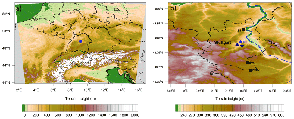
Figure 1 Model domain 1 (a) and domain 3 (b). The blue dot in panel (a) denotes Stuttgart. Black dots in panel (b) show the location of the meteorological measurement sites. The diamonds in panel (b) denotes the Neckartor (NT) and Schlossplatz (SP) locations and the blue contour line denotes the Neckar River (river data © OpenStreetMap contributors 2020. Distributed under a Creative Commons BY-SA License).

Fallmann et al. (2016) and Kuik et al. (2016) performed air quality simulations with WRF-Chem over the cities of Berlin and Stuttgart on a CP resolution down to 1 km and less than 40 model levels. They used the Netherlands Organisation for Applied Scientific Research – Monitoring Atmospheric Composition and Climate (TNO-MACC) emission inventory (Kuenen et al., 2014), which is available as an annual total on a 7 km × 7 km resolution. As the topography of Stuttgart is very complex, the AQFS applies the WRF-Chem model on a TP horizontal resolution using 100 model levels to account for the shallow boundary layer occurring during wintertime. In addition, we applied a local emission data set from the Baden-Württemberg State Institute for the Environment, Survey and Nature Conservation available as annual mean on a horizontal resolution of 500 m × 500 m to resolve fine-scale emission structures.

Our study focuses on the methodology how to set up a AQFS prototype by using WRF-Chem and its application to a typical wintertime situation during January 2019 in the Stuttgart metropolitan area. The paper is set up as follows: Sect. 2 describes the design of our AQFS model system on the TP resolution of 50 m, followed by a description of the selected case study. Section 4 shows the results with respect to meteorological variables and air quality including a discussion. Section 5 summarizes our work and provides an outlook on potential future enhancements of the AQFS prototype.

2 AQFS design

2.1 WRF model setup

For our AQFS prototype, we selected the Advanced Research WRF-Chem model version 4.0.3 (Grell et al., 2005; Skamarock et al., 2019). To reach the targeted resolution of 50 m, three model domains have been applied, with horizontal resolutions of 1250, 250, and 50 m, and encompass 800 × 800 grid cells in the outer domain and 601 × 601 grid cells in the two inner TP domains. The reasons for starting with a resolution of 1250 m in the outermost domain are (1) to avoid the application of a convection parametrization which can deteriorate the model results (Prein et al., 2015; Coppola et al., 2020), (2) so that the model starts to partially resolve turbulent structures, whilst a planetary boundary layer (PBL) parametrization is still necessary (Honnert and Masson, 2014; Honnert et al., 2020), and (3) to reach the target resolution with a nesting ratio of 5:1. The areas of model domains 1 and 3 are shown in Fig. 1.

As seen from Fig. 1b, the Stuttgart metropolitan area is characterized by an elevation variation of more than 300 m. The lowest elevation is approximately 220 m in the basin, while the highest elevation reaches up to 570 m. As the main traffic roads are in the basin, especially during wintertime, this often leads to a worsening of the air quality as the surrounding prevents an air mass exchange due to the stationary temperature inversion.

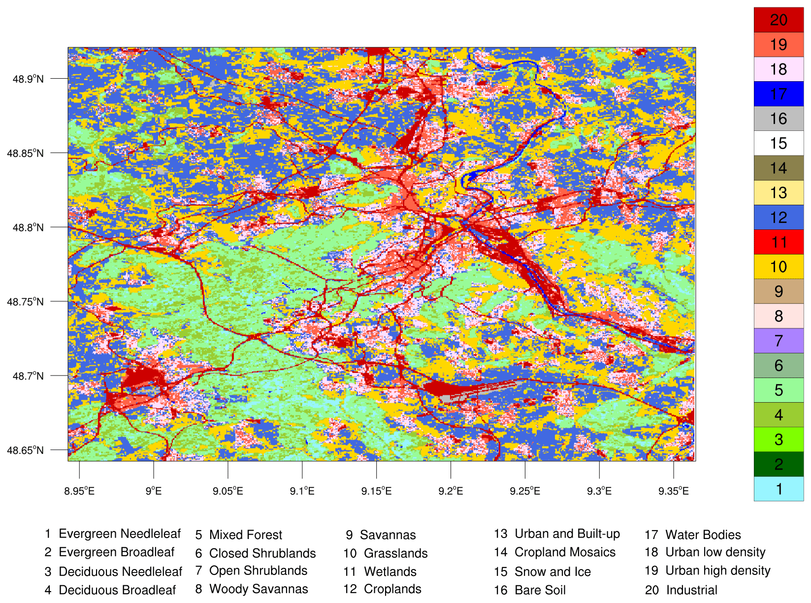
Figure 2 Land cover data from the Baden-Württemberg State Institute for the Environment (LUBW) reclassified for WRF in the innermost domain at a resolution of 50 m.

For the WRF model system, land cover and soil texture fields are not available at resolutions higher than 500 m. Therefore, we reclassified land cover data from the Copernicus Coordination of Information on the Environment (CORINE) Land Cover (CLC) 2012 data set (European Union, 2012), available on a resolution of 100 m, from the original 44 categories to the categories applied in the WRF model for the simulations of the outer two domains. For the innermost model domain, we incorporated the most recent high-resolution land cover data set from the Baden-Württemberg State Institute for the Environment (LUBW), which was derived from Landsat (Butcher et al., 2019) in 2010 and is available at 30 m resolution (https://udo.lubw.baden-wuerttemberg.de/public/, last access: 23 March 2021). This data set was also reclassified to the corresponding land cover categories used in WRF and is shown in Fig. 2.

The resolution of the provided default Food and Agriculture Organization of the United Nations (FAO) soil texture data is only 10 km; therefore, we used soil texture data from the International Soil Reference and Information Centre (ISRIC) SoilGrids project (Hengl et al., 2014, 2015). These data are available on a resolution of 250 m. Terrain information was provided by the National Center for Atmospheric Research (NCAR) derived from the global multi-resolution terrain elevation data 2010 (GMTED2010) data set (Danielson and Gesch, 2011) for domain 1. As the horizontal resolution of the GMTED2010 data set is 1 km, the 3 arcsec gap-filled Shuttle Radar Topography Mission (SRTM) data set (Farr et al., 2007) is used for domain 2. As this resolution is still too coarse for our targeted resolution of 50 m, the European Union digital elevation model (EU-DEM; European Union, 2017), available at a resolution of 25 m, is used for the innermost domain.

In our setup, we use 100 vertical levels for all domains using the traditional terrain following coordinate system in WRF; 20 of the levels are distributed in the lowest 1100 $\mathrm{m}\mathrm{a}.\mathrm{g}.\mathrm{l}.$ (above ground level). All domains apply the Noah-MP land surface model (Niu et al., 2011; Yang et al., 2011), the revised MM5 (Fifth-Generation Penn State/NCAR Mesoscale Model) surface layer scheme based on Monin–Obukhov similarity theory (Jiménez et al., 2012), the Thompson two-moment cloud microphysics scheme (Thompson et al., 2008), and the Rapid Radiative Transfer Model for GCMs (RRTMG; Iacono et al., 2008) for parametrizing longwave and shortwave radiation. Due to the coarser resolution of the outermost domain, we applied the Yonsei University (YSU; Hong et al., 2006) PBL parametrization in D01 only. As suggested by the WRF user guide, we applied the subgrid turbulent stress option for momentum (Kosovic, 1997) in domains 2 and 3. The complete namelist settings are provided in the Supplement.

The more sophisticated building effect parameterization (BEP; Martilli et al., 2002) is not applied, as this scheme does not work with our selection of parameterizations. Instead, the single-layer urban canopy model (UCM) (Kusaka and Kimura, 2004) is selected to improve the representation of the urban canopy layer and the surface fluxes. The parameters needed by the UCM are read in from the lookup table (URBPARAM.TBL), which was adjusted for the Stuttgart area following Fallmann (2014).

Atmospheric chemistry is parameterized by the Regional Acid Deposition Model second generation (RADM2) model (Stockwell et al., 1990). RADM2 features more than 60 chemical species and more than 135 chemical reactions including photolysis. Aerosols are represented by the Modal Aerosol Dynamics Model for Europe (MADE) and Secondary Organic Aerosol Model (SORGAM) scheme (Ackermann et al., 1998; Schell et al., 2001) considering size distributions, nucleation, coagulation, and condensational growth. The combination of RADM2–MADE–SORGAM is a computationally efficient approach and is widely used for simulations over Europe (Forkel et al., 2015; Mar et al., 2016). To further enhance vertical mixing of CO to higher altitudes during nighttime over urban grid cells, the “if” statements in the dry deposition driver of WRF-Chem at lines 690 and 707 have been deleted accordingly, as shown in the Supplement of Kuik et al. (2018).

Compared to a previous study from Fallmann et al. (2016), who performed simulations over the Stuttgart metropolitan area using WRF-Chem on a CP resolution of 3 km, or the study of Kuik et al. (2016), who performed a 3-month simulation at different resolutions over Berlin, simulations on the TP resolution provide a much more realistic representation of the land cover structures (see Fig. 2 in this paper and, e.g., Fig. 2b in Fallmann et al., 2016). As the climate in the Stuttgart metropolitan area is strongly influenced by the topography, we are convinced that our special combination of a TP resolution and high-resolution emission data (see Sect.  2.3) will lead to a better understanding and prediction of the air pollution situation in this area.

Currently, air pollution modeling with WRF-Chem is a computationally expensive task. Depending on the number of output variables and frequency (5 min in our study), a 24 h simulation currently takes around 36 h wall-clock time. For future experiments, it is worth trying the I/O quilting option in combination with PnetCDF, which should considerably reduce the time spent on I/O.

While the WRF model itself is ready for hybrid parallelism (MPI plus OpenMP), the WRF-Chem model can only be used with MPI. If WRF-Chem could be enhanced for additional OpenMP capabilities, this would lead to an increase in computation speed that is almost linear with the number of OpenMP threads.

Due to the complexity of the chemistry model in combination with the very high horizontal resolution and the calm meteorological conditions, the adaptive model time step option was chosen instead of a fixed time step. Model output is available in 5 min intervals for the innermost model domain.

Our single-day case study on the TP scale is designed to serve as a test bed to set up an air quality forecasting system prototype for the Stuttgart metropolitan area. For process studies, the model chain itself can be applied to other areas over the globe as long as (1) detailed land cover and soil texture data are available and (2) high-resolution emission data not only from traffic are available. The new model system can be even applied in a forecast and warning mode if near-real-time emissions as well as meteorological and chemical input data are available in a timely manner. As the computational demands of applying WRF-Chem on the TP scale are very high, access to an high-performance computing (HPC) system is a prerequisite.

2.2 Model initialization

The meteorological initial and boundary conditions were provided by the operational ECMWF integrated forecasting system (IFS) analysis on model levels. The IFS is a global model with 9 km horizontal resolution and applies a sophisticated four-dimensional variational (4D-Var) data assimilation system (Bonavita et al., 2016). The data have been retrieved from the ECMWF Meteorological Archival and Retrieval System (MARS) and were interpolated to a resolution of 0.05^∘.

The initialization and provision of the boundary conditions of the chemistry of the model are done with data from the Whole Atmosphere Community Climate Model (WACCM; Marsh et al., 2013) using MOZART conversion tool (MOZBC) (Pfister et al., 2011). As the resolution of WACCM is very coarse, the input data were enhanced by the ECMWF Copernicus Atmosphere Monitoring Service (CAMS) reanalysis data set on 60 model levels and 40 km horizontal resolution (Inness et al., 2019).

2.3 Emission data

The emission data set used in this study is a combination of three products. Global input data sets containing coarse resolution emissions from different sources are obtained from the Brazilian developments on the Regional Atmospheric Modeling System (BRAMS) numerical modeling system (Freitas et al., 2017). The PREP-CHEM-SRC tool (Freitas et al., 2011) is then applied as pre-processor to convert these emissions to the appropriate WRF units and interpolate the data onto the WRF model grid.

As global emission data sets have a very coarse resolution in space and time, higher-resolution emission data for Europe from the CAMS-REG-AP product (Copernicus Atmosphere Monitoring Service – CAMS; Copernicus, 2020) became available (Granier et al., 2019). Its resolution is approximately 7 km × 7 km, and it is based on total annual emissions from 2016. This product provides emissions of PM₁₀, PM_2.5, SO₂, CO, NO_x, and CH₄ and contains sources from different sectors, separated into 10 different categories following the Gridded Nomenclature For Reporting (GNFR; Granier et al., 2019).

The third emission data set (BW-EMISS) deployed in our study was obtained from the LUBW. This data set contains annual mean emissions from different sectors following the GNFR classification, and it is currently available only until 2014 and has a horizontal resolution of 500 m. Unfortunately, more recent quality-controlled data sets were not available when our study was performed. It is expected that annual emissions for 2018 will become available by mid-2021.

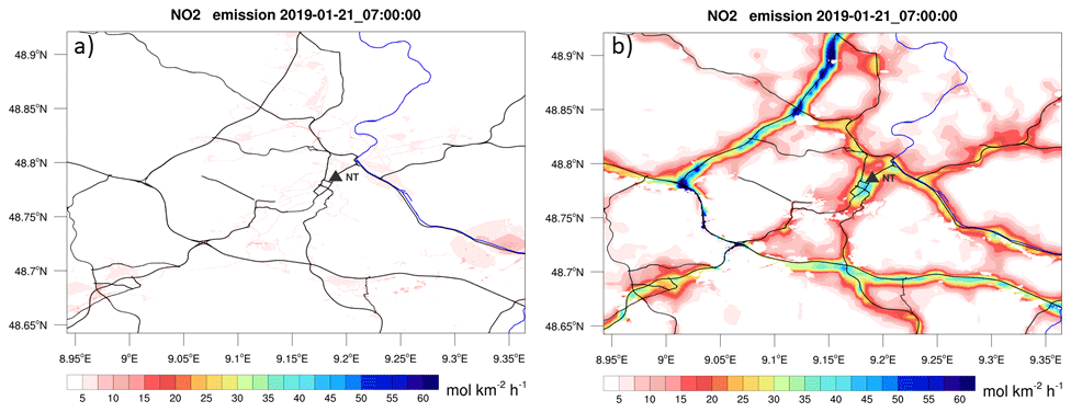
Figure 3 NO₂ emissions valid at 07:00 UTC on 21 January 2019. Panel (a) shows the emissions derived from the CAMS-REG-AP data set and (b) shows the emissions derived from the BW-EMISS data set (map data © OpenStreetMap contributors 2020. Distributed under a Creative Commons BY-SA License).

As CAMS-REG-AP and BW-EMISS only contain annual sums or annual mean values, a temporal decomposition was applied for both data sets following Denier van der Gon et al. (2011). Depending on the GNFR code, the data are first projected onto the corresponding month, followed by the corresponding day of the week and the hour of the day. A similar approach was performed, e.g., in Resler et al. (2020, under review) for the city of Prague. After finishing the decomposition, the data were converted to the corresponding units and interpolated onto the WRF model grid using the Earth System Modeling Framework (ESMF; Valcke et al., 2012) interpolation utilities.

Figure 3 shows an example of the NO₂ emissions derived from the CAMS-REG-AP product (Fig. 3a) and the emission data derived from the LUBW data set (Fig. 3b) on 21 January 2019 at 07:00 UTC.

Due to its much higher horizontal resolution, the BW-EMISS data set (Fig. 3b) shows much more detailed structures for the NO₂ emissions which are mainly caused by road traffic. The average emissions for this particular time step are 2 $\mathrm{mol}{\mathrm{km}}^{-\mathrm{2}}{\mathrm{h}}^{-\mathrm{1}}$ for the CAMS-REG-AP data set and 7 $\mathrm{mol}{\mathrm{km}}^{-\mathrm{2}}{\mathrm{h}}^{-\mathrm{1}}$ for the BW-EMISS data set.

In addition, the following adjustments have been performed: (1) NO_x emissions from forest grid cells have been reduced by 90 %, (2) road traffic NO_x emissions were transformed into 90 % NO and 10 % NO₂ emissions following Kuik et al. (2018), (3) all emissions from Stuttgart Airport were reduced by 90 % during the nighttime flight ban between 00:00 and 04:00 UTC as well as after 21:00 UTC.

Figure 4 Workflow of the AQFS prototype system.

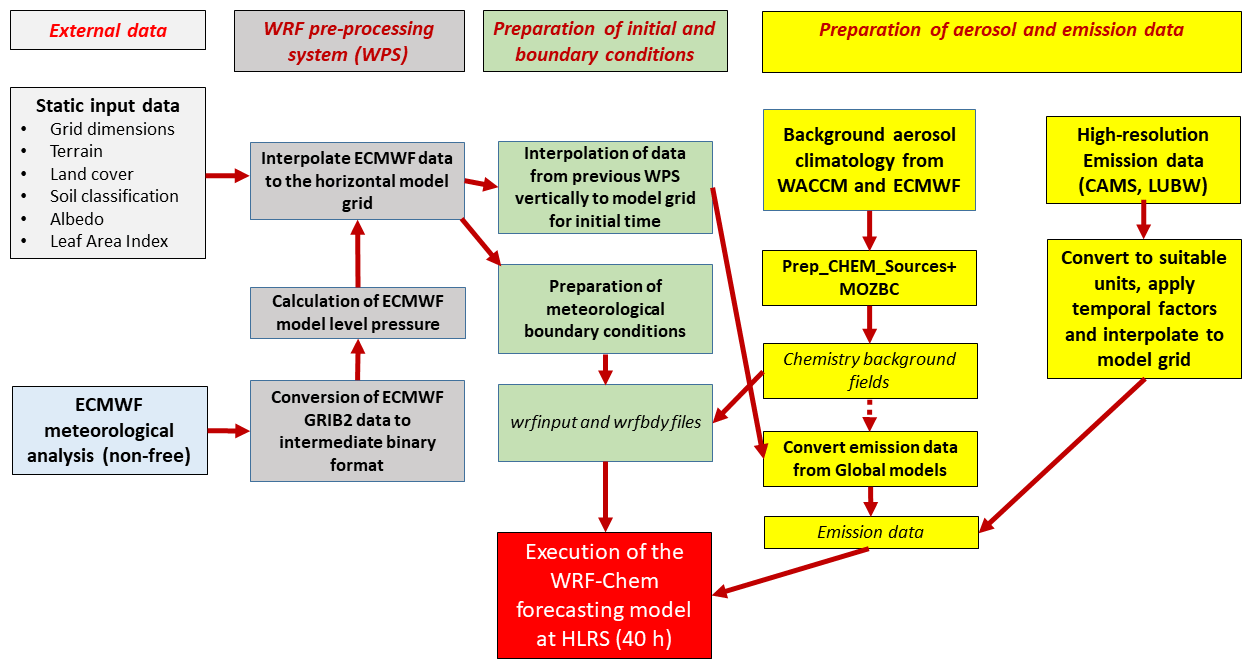
The WRF-Chem model only ingests one emission data set per species; hence, emissions from the different GNFR categories have accumulated in a single emission data set before performing the simulation. Figure 4 summarizes all necessary steps and the complete data and workflow of the AQFS prototype.

2.4 Observations

We used data from three meteorological stations: Stuttgart-Schnarrenberg (48.8281^∘ N, 9.2^∘ E; elevation 314 m), Stuttgart Airport (48.6883^∘ N, 9.2235^∘ E; elevation 375 m), and the Institute of Physics and Meteorology (IPM) at the University of Hohenheim (48.716^∘ N, 9.213^∘ E; elevation 407 m) to validate the simulated 2 m temperatures; data are available every 10 min. The locations are indicated by the black dots in Fig. 1b. In addition, the radiosonde data from Stuttgart-Schnarrenberg were used.

3 Case study description

For our study, we selected 21 January 2019. This day was characterized as “fine dust alarm” situation (Stuttgart Municipality and German Meteorological Service (DWD), 2019), which is defined by a combination of the following criteria:

1. expected daily maximum PM₁₀ concentration at Stuttgart Neckartor (NT in Fig. 1b) is higher than 30 µg m⁻³;

2. no rain on the following day;

3. 10 m wind speed less than 3 m s⁻¹ from the south to northwest directions (180–330^∘);

4. nocturnal atmospheric inversion;

5. mixing layer depth less than 500 m during the day;

6. daily average 10 m wind speed less than 3 m s⁻¹ from all directions.

A sufficient criterion is a higher PM₁₀ concentration following (1). If (1) is not fulfilled, then (2) and (3) together with either (4) and/or (5) have to be fulfilled. If only (4) or (5) is fulfilled, then (6) has to be considered. For our case study, criteria (1)–(5) were fulfilled.

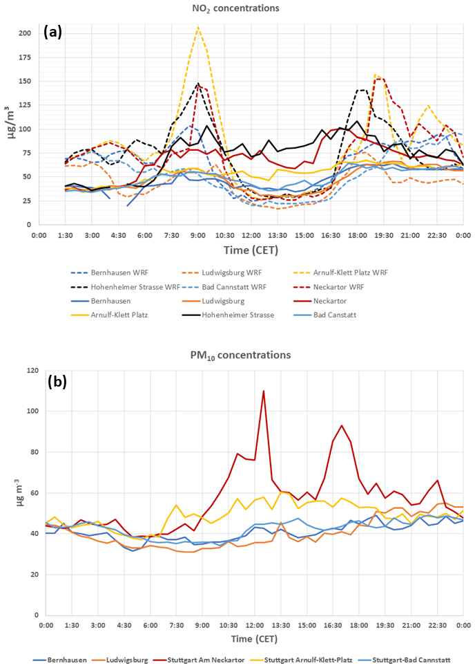
Figure 5 NO₂ (a) and PM₁₀ (b) concentrations at several stations distributed over the model domain on 21 January 2019. The dashed line in panel (a) denotes the simulated NO₂ concentration and the time zone (CET) corresponds to local time. Measurements at Neckartor, Hohenheimer Strasse, and Arnulf-Klett Platz are directly taken next to the main road.

The solid lines in Fig. 5 show the observed PM₁₀ and NO₂ concentrations at several stations in our model domain. From Fig. 5a, the high NO₂ concentrations at Neckartor and Hohenheimer Strasse occurring after sunrise can be clearly identified. While these measurements are taken next to main roads, the other stations show considerably lower NO₂ concentrations throughout the day. The PM₁₀ concentrations (Fig. 5b) show extremely high values at Neckartor, exceeding 100 µg m⁻³ around noon and the evening rush hour which clearly meets the main criteria of the “fine dust alarm” situation. The other stations, which are not directly located near main roads with heavy traffic, show considerably lower PM₁₀ concentrations around 40 µg m⁻³ .

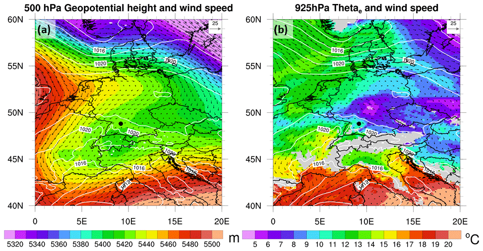
Figure 6 (a) ECMWF operational analysis of 500 hPa geopotential height, sea level pressure (white contour lines) together with 500 hPa wind velocities valid at 00:00 UTC on 21 January 2019. Panel (b) shows the 925 hPa equivalent potential temperature together with 925 hPa wind velocities and sea level pressure (white contour lines). Gray areas indicate values below the ECMWF model terrain. The black dot denotes Stuttgart, and the reference wind vector length (top right corner of each figure) is equal to 25 m s⁻¹.

This day was a typical winter weather situation. Central Europe was located at the east flank of a blocking high-pressure system located over the eastern Atlantic together with moderate to low horizontal geopotential gradients and resulting weak winds at 500 hPa in southwestern Germany (Fig. 6a).

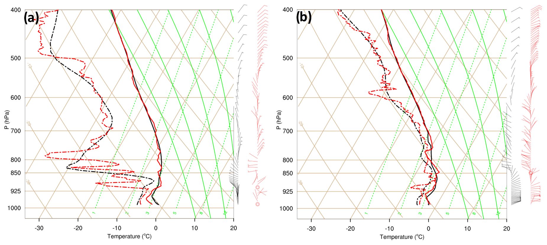
Figure 7 Comparison of temperature, dew-point and wind of the WRF model simulation (black line) and the sounding from Stuttgart-Schnarrenberg (red line) valid at 00:00 UTC (a) and 11:00 UTC (b) on 21 January 2019. The solid lines denote the temperature profile and the dash-dotted line denotes the dew-point profile. Wind barbs denote wind speed in m s⁻¹.

Near-surface temperatures are below freezing level, between 1000 and 850 hPa very light easterly winds characterize the flow, and a dry layer is present around 925 hPa (Fig. 6b). Above 850 hPa, the wind direction rapidly changes to westerly directions, but the wind speeds remain below 5 m s⁻¹ (see Fig. 7a).

The inversion between the two air masses inhibits vertical mixing, leading to higher concentrations of aerosols in the lowest few hundred meters above ground level (AGL) and preventing air mass exchange aloft. This inversion is further enhanced by the special orography of the city of Stuttgart.

4 Results and discussion

4.1 Meteorological quantities

Figure 7a shows a Skew-T diagram of the model initial conditions (black line) at Stuttgart-Schnarrenberg valid at 00:00 UTC on 21 January 2019 in comparison with the observations (red line).

The initial conditions agree well with the sounding showing a weak temperature inversion around 900 hPa with high relative humidity values up to 650 hPa. The observed and simulated lifting condensation level is 940 hPa and the integrated water vapor (PWAT) is 8 mm. Wind speed and direction agree with the observations, showing a wind shear above 850 hPa associated with low wind speeds of less than 5 m s⁻¹.

To further evaluate the stratification conditions during the day, Fig. 7b shows the observed and simulated temperature, dew point, and wind profiles at 11:00 UTC. The vertical structure of the observation and the simulation has an almost perfect agreement. The temperature inversion layer at 910 hPa is well captured, although the simulated temperatures below the inversion are too high by about 1.5 K. The humidity profile (expressed as a dew-point profile) is also very well captured with the largest moisture content below 870 hPa. Wind speed and direction above 850 hPa agree well with the observation throughout the atmosphere. With regard to the vertical model resolution, the wind situation in the lowest 1000 $\mathrm{m}\mathrm{a}.\mathrm{g}.\mathrm{l}.$ is also reasonably represented.

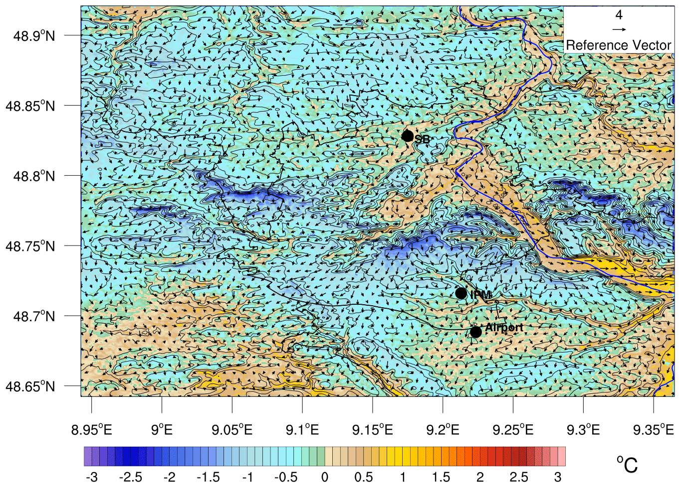
Figure 8 The 2 m temperature together with 10 m wind velocities at 12:00 UTC on 21 January 2019. The thick black line denotes the Stuttgart city limits and the thin black contour lines denote the terrain. The blue line denotes the Neckar River (river data © OpenStreetMap contributors 2020. Distributed under a Creative Commons BY-SA License).

Figure 8 exemplarily shows the simulated 2 m temperature together with 10 m wind velocities at 12:00 UTC (noon) to display the complexity of the Stuttgart metropolitan area.

The 2 m temperatures show a daytime warming of downtown Stuttgart and the Neckar Valley, while temperatures slightly below 0 ^∘C are still present at higher elevations (blue colors in Fig. 8). The wind situation is very complex due to weak wind speeds in combination with a shallow boundary layer (see Fig. 16), but the wind flow along the upper Neckar River (south of 48.75^∘ N) is strongly pronounced. After sunset, wind speed starts to decrease and the channeling effect along the Neckar weakens (not shown).

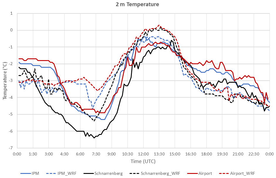
Figure 9 Diurnal cycle of 2 m temperatures for the three meteorological stations shown in Fig. 1b. Solid lines denote the observation; dashed lines denote the model simulation. The temporal resolution of the data points is 10 min.

Figure 9 shows an evaluation of the diurnal cycle of 2 m temperatures at the three measurement sites Schnarrenberg, IPM and airport. Sunrise is at 07:00 UTC and sunset at 16:00 UTC, and the model data are averaged over five grid cells around the measurement site to take into account that even a simulation with 50 m resolution cannot fully capture the local conditions at the measurement site. The northern station (Schnarrenberg) shows a lower temperature throughout the day than the other two stations, which are situated 3 km apart at a similar elevation. The temperature is about 1 K colder during the day and 0.5 K colder during the night.

At Schnarrenberg, the observed diurnal cycle is reasonably well simulated with WRF. Between 00:00 and 15:00 UTC, a warm temperature bias of 1 K is present in the simulation, which turns into a small negative bias after sunset. At IPM, the simulation shows a cold bias until 04:00 UTC turning into a warm bias as the strong temperature drop is not simulated until 06:30 UTC. After 09:00 UTC until sunset, the simulated temperature agrees well with the observations, while later a cold bias of around 1 K is present.

For the airport station, the model stays too warm with a positive bias of almost 2 K between 05:00 and 09:00 UTC. During the further course of the day, the bias reduces to 1 K at noon, while after sunset it turns into a negative bias of 1 K.

A possible reason for the larger differences at the airport and IPM before (after) sunrise (sunset) is the observed occurrence of low stratus or fog. At the beginning of the simulation, cloud coverage was reported by 5–7 oktas (broken clouds) over Schnarrenberg and the airport at approximately 500 $\mathrm{m}\mathrm{a}.\mathrm{g}.\mathrm{l}.$ (not shown), while after 04:00 UTC the low-level clouds started to diminish at Schnarrenberg, leading to a strong cooling until the early morning, which is seen as a temperature decrease in the observations shown in Fig. 9. The temperature drop at Schnarrenberg and IPM is also simulated but with a delay of approximately 2 h. A reason for this delayed temperature drop could be a simulated thin cloud layer around 1000 $\mathrm{m}\mathrm{a}.\mathrm{g}.\mathrm{l}.$, which is present in the lower left and partly the lower right quadrant of the model domain. This cloud layer slowly moves in a southeasterly direction and starts to dissolve around 06:00 UTC.

During the evening transition and the following night, the low stratus develops again at the measurement sites with a ceiling of 500 $\mathrm{m}\mathrm{a}.\mathrm{g}.\mathrm{l}.$ but is not simulated and thus contributes to a stronger cooling in the model. Another contributing factor to the delayed cloud dissipation could be the turbulence spin-up time (Kealy et al., 2019), but this is beyond the scope of this study.

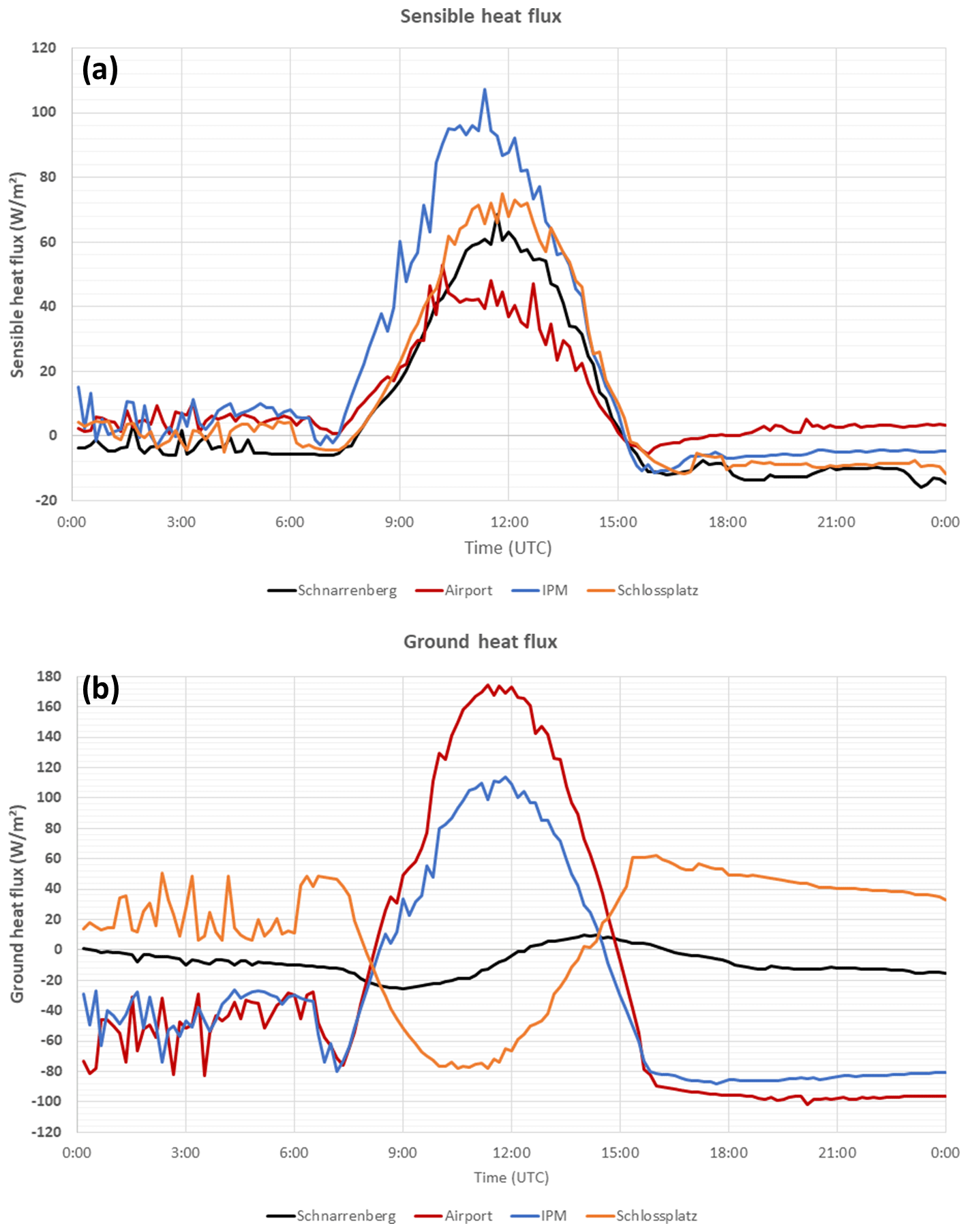
Figure 10 Diurnal cycle of simulated sensible heat flux (SH, a) and ground heat flux (GRDFLX, b) at the four stations: Schnarrenberg, Stuttgart Airport, IPM, and Schlossplatz (Fig. 1b). Positive values of GRDFLX indicate fluxes into the soil. The land cover categories are bare soil (airport), croplands (IPM), low-density residential (Schnarrenberg), and high-density residential (Schlossplatz).

Although no measurements of sensible heat and ground heat fluxes are available, diurnal cycles of the fluxes at the locations IPM, Schnarrenberg, airport, and Schlossplatz were investigated. Figure 10 shows the simulated surface sensible heat and ground heat flux at the four sites.

The sensible heat flux (Fig. 10a) shows a typical diurnal cycle with fluxes around zero before (after) sunrise (sunset). During the day, the model simulates typical wintertime sensible heat fluxes between 40 and 100 W m⁻² (e.g., Zieliński et al., 2018), which nicely shows a dependency on the different underlying land cover types. Lower sensible heat fluxes occur over the sparsely vegetated surface at the airport as compared to the cropland station IPM, while the urban locations (Schnarrenberg and Schlossplatz) show interjacent values. As the algorithm to diagnose the 2 m temperature in Noah-MP is rather complex, no clear correlation between SH and the 2 m temperature shown in Fig. 9 can be made. The latent heat fluxes (not shown) are almost zero at Schnarrenberg and less than 10 W m⁻² at the other two locations due to cold and dry winter conditions.

The simulated ground heat flux (Fig. 10b) shows an interesting behavior. Until sunrise, the simulated GRDFLX at the airport and IPM shows fluctuations around −50 W m⁻², indicating some low-level clouds in accordance with the too-high simulated 2 m temperatures shown in Fig. 9. During the further course of the day, IPM and airport show a clear diurnal cycle with maximum values between 100 and 170 W m⁻² reflected in the highest surface temperatures during the day (not shown).

At Schnarrenberg, most of the time the ground heat flux is less than zero, indicating a cooling of the soil, while between 12:00 and 16:00 UTC small positive values are simulated. As Schnarrenberg is categorized as a low-density residential area (category 31) with an urban fraction of 0.5 and the UCM is applied here, energy is mainly stored in the urban canopy layer instead of being transferred into the soil. At Schlossplatz (high-density residential area), the ground heat flux shows a similar shape but with a larger amplitude compared to Schnarrenberg.

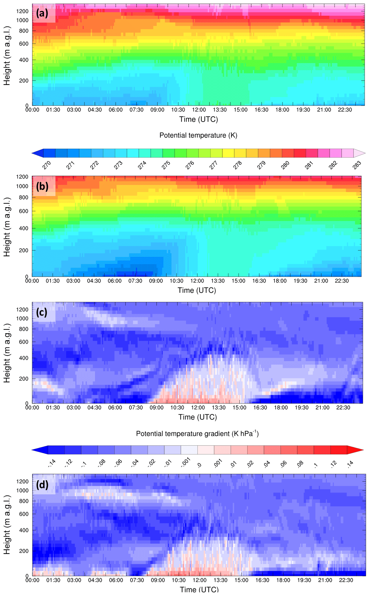
Figure 11 Time–height cross section of the simulated potential temperature at Schnarrenberg (a) and IPM (b). Panels (c) and (d) show the potential temperature gradient at Schnarrenberg (c) and IPM (d). The displayed altitude is above ground level.

As this day was characterized by a shallow PBL and a temperature inversion, it is worth investigating the PBL evolution during the day. Figure 11a and b show time–height cross sections of potential temperature at IPM (top) and Schnarrenberg (bottom).

Both locations are characterized by a very stable shallow boundary layer until 09:00 UTC with a depth of less than 200 m. Between 03:00 and 09:00 UTC, the temperatures at Schnarrenberg are up to 1.5 K colder near the surface (Fig. 9), resulting in a stronger potential temperature gradient up to 400 $\mathrm{m}\mathrm{a}.\mathrm{g}.\mathrm{l}.$ compared to the IPM location. During the day, the boundary layer height increases to 400 $\mathrm{m}\mathrm{a}.\mathrm{g}.\mathrm{l}.$, as indicated by the constant potential temperature (e.g., Bauer et al., 2020), which is a typical value for European winter conditions (Seidel et al., 2012; Wang et al., 2020). The PBL heights are also visible by the potential temperature gradients (Δθ) shown in Fig. 11c and d. During the morning hours, a very shallow boundary layer was simulated at Schnarrenberg (blue colors in Fig. 11c), while at IPM some fluctuations are present. During daytime, Δθ nicely shows the PBL height evolution up to 400 $\mathrm{m}\mathrm{a}.\mathrm{g}.\mathrm{l}.$, while after sunset the PBL collapses to a very stable layer again (dark blue colors in Fig. 11c and d) with heights between 50–100 $\mathrm{m}\mathrm{a}.\mathrm{g}.\mathrm{l}.$ Calculating the gradient Richardson number (Ri; Chan, 2008) (not shown) and assuming a threshold of 0.25 for a turbulent PBL (Seidel et al., 2012; Lee and Wekker, 2016) leads to similar results After sunset at around 15:30 UTC, the boundary layer collapses to a nighttime stable boundary layer and a temperature inversion occurs again.

4.2 Evaluation of NO₂ and PM₁₀

The most relevant air pollutants for air quality considerations in cities are NO₂ and PM₁₀. Sources for these are mainly truck supply, transit, and commuter traffic through the city as well as advection from motorways south, west, and northwest of Stuttgart.

As the incorporated emissions are from 2014 and are based on annual values, it cannot be expected that the model exactly matches the observed concentrations. For instance, the actual traffic, the sequence of traffic lights, and traffic congestions of this particular day cannot be realistically represented. In addition, all diagnosed or prognostic chemical quantities are only available on model levels. For TP applications with WRF, selecting the lowest model half level being at ∼ 15 m above ground is a reasonable choice (Bauer et al., 2020).

We start with the discussion of the simulated horizontal distributions followed by vertical cross sections of NO₂ and PM₁₀.

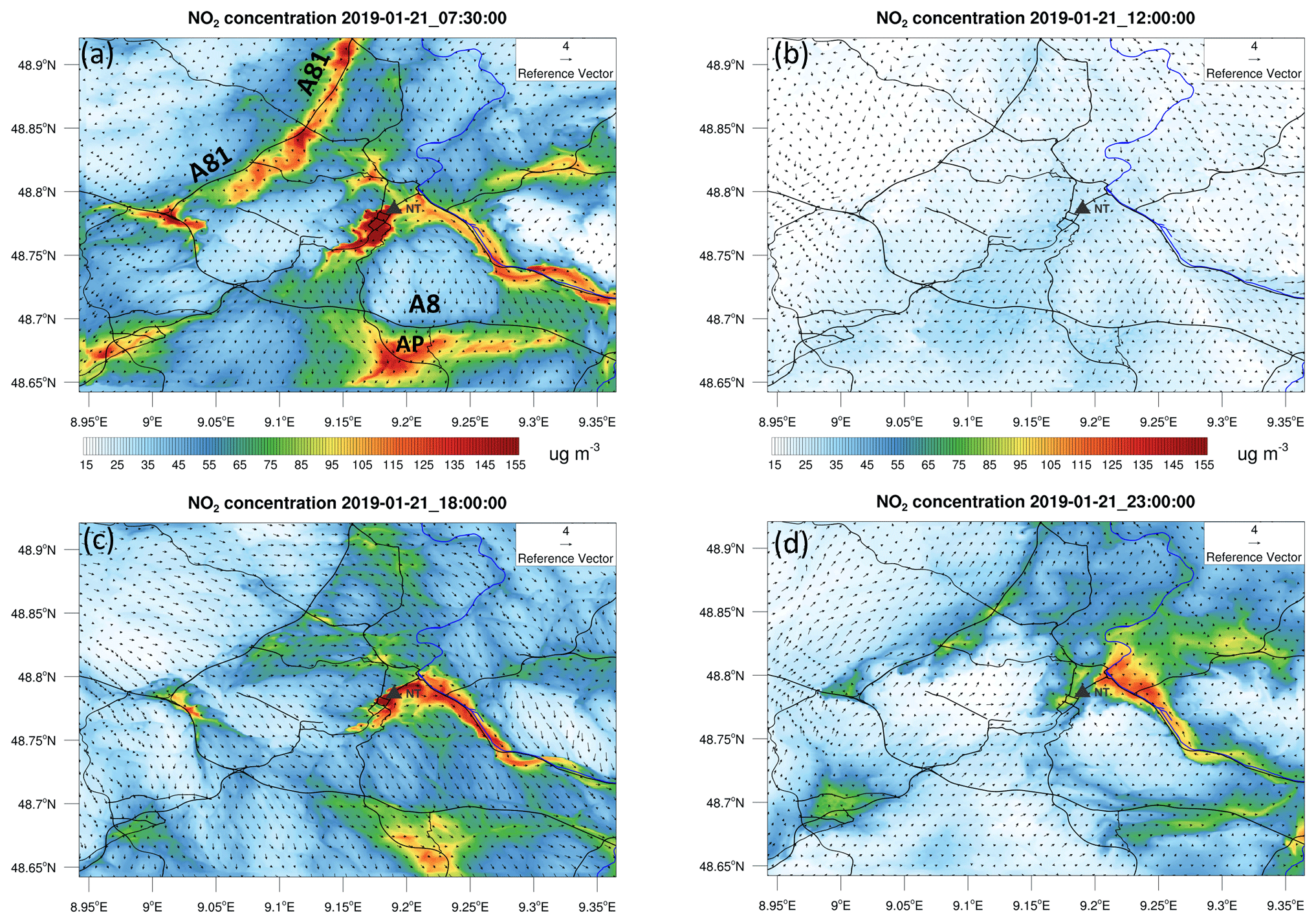
Figure 12 NO₂ concentration at the lowest model level for 07:30, 12:00, 18:00, and 23:00 UTC (a–d) on 21 January 2019. The black contour lines denote main roads and motorways in and around Stuttgart (map data © OpenStreetMap contributors 2020. Distributed under a Creative Commons BY-SA License). AP denotes the airport; A8 and A81 denote the main motorways around Stuttgart.

4.2.1 Horizontal distribution

Figure 12 shows the horizontal distribution of the NO₂ concentration at the lowest model half level (∼ 15 $\mathrm{m}\mathrm{a}.\mathrm{g}.\mathrm{l}.$) at four time steps (07:30, 12:00, 18:00, and 23:00 UTC) on 21 January 2019.

At 07:30 UTC, the morning traffic rush hour is visible in the NO₂ concentrations in Fig. 12a. High NO₂ concentrations of more than 80 µg m⁻³ are simulated along the A81 motorway in the northwest of the domain, over the airport and over downtown Stuttgart. In the Neckar Valley, the concentrations exceed 120 µg m⁻³. At noon (Fig. 12b), when turbulence is fully evolved (Fig. 11), the simulated NO₂ concentrations are less than 30 µg m⁻³ on average apparently due to vertical mixing of NO₂ (see the next section). In the evening (Fig. 12c), the simulated NO₂ concentrations increase again, showing values of more than 100 µg m⁻³ over the airport and more than 150 µg m⁻³ in downtown Stuttgart and the Neckar Valley due to road and air traffic. The high morning concentrations along the northwestern motorway are not reached since the wind speed increases and the near-surface winds turn towards a westerly direction. According to the emission data set converted by the temporal factors, the evening traffic spreads over a longer time. During the night (Fig. 12d), NO₂ accumulates in the Stuttgart basin as well as the Neckar Valley due to the very low nocturnal boundary layer height of less than 200 m capped by an atmospheric inversion (Fig. 11).

Compared to the observed NO₂ concentrations (Fig. 5a), the simulated concentrations during the peak traffic times are too high at Arnulf-Klett Platz, Neckartor, and Hohenheimer Strasse. Possible reasons are that either the traffic is reduced and/or that the vehicle emission classifications have been improved since 2014. Another contributing factor could be that the vertical mixing near the surface is too weak during sunrise and sunset, while it appears slightly too strong during daytime, as indicated by the very low simulated NO₂ concentrations.

Apart from NO₂, the concentration of PM₁₀ is an important parameter for air quality considerations and is the decisive factor for proclaiming a “fine dust alarm” situation in Stuttgart (Stuttgart Municipality and German Meteorological Service (DWD), 2019).

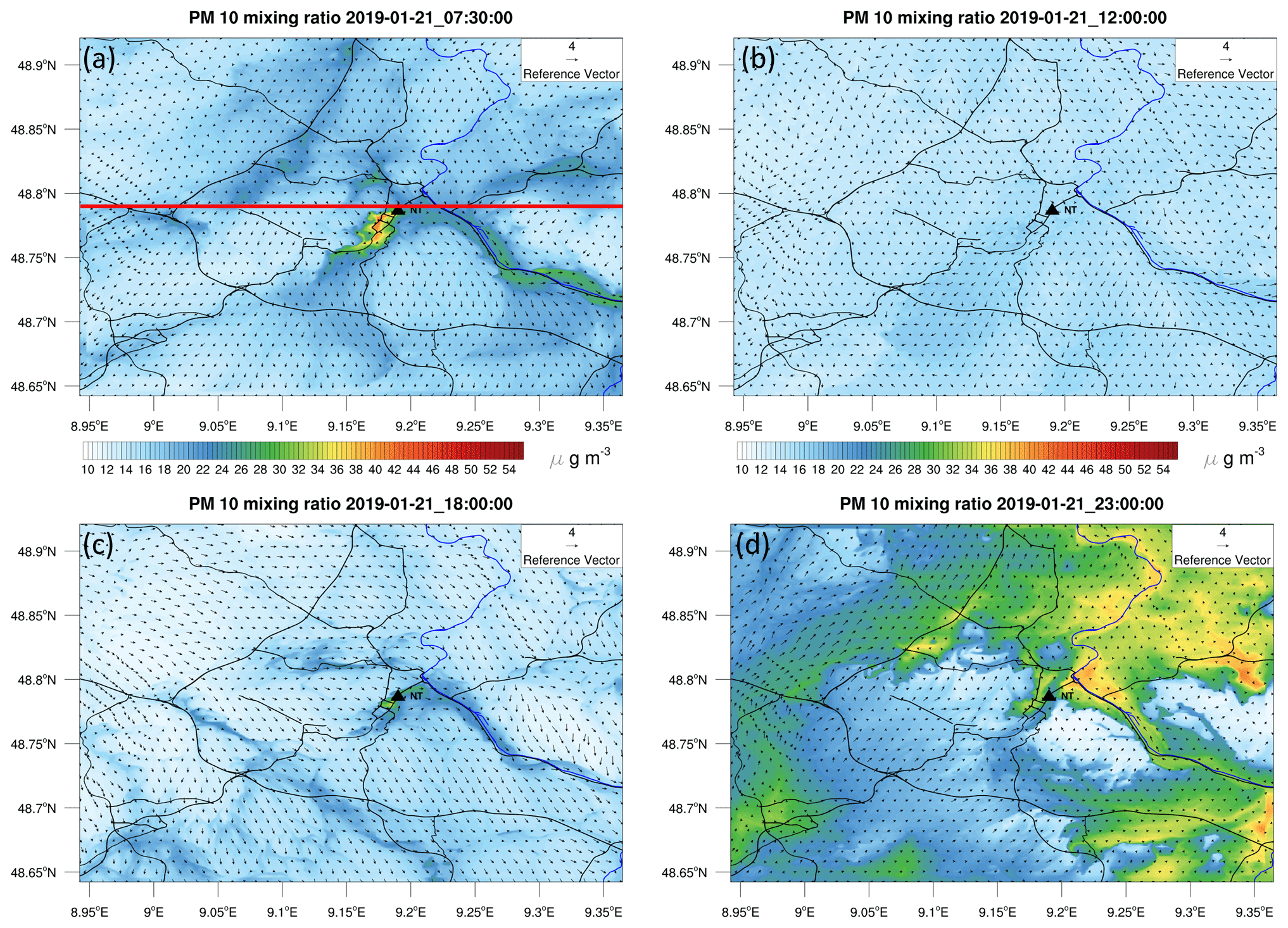
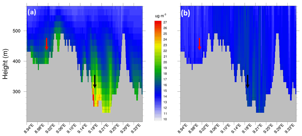
Figure 13 Same as Fig. 12 but for PM₁₀ (map data © OpenStreetMap contributors 2020. Distributed under a Creative Commons BY-SA License). The red line in panel (a) denotes the cross section shown in Figs. 14 and 15.

Figure 13 shows the horizontal distribution of PM₁₀ for the same time steps as those shown in Fig. 12.

During the morning traffic (Fig. 13a), PM₁₀ accumulates in the Stuttgart basin, as this is an area with heavy traffic during the morning and an atmospheric inversion is present (Fig. 7). Interestingly, the high NO₂ concentrations along the motorway (Fig. 12a) do not lead to very high PM₁₀ concentrations potentially due to chemical transitions caused by low temperatures.

During daytime, when turbulence is fully evolved, the concentration of PM₁₀ decreases to less than 20 µg m⁻³ due to vertical mixing and horizontal transport (see the next section). After sunset (Fig. 13c), PM₁₀ starts to accumulate again in the Stuttgart basin showing concentrations between 35–40 µg m⁻³. During the night (Fig. 13d), PM₁₀ accumulates over a large part of the model domain as the nocturnal boundary layer is very shallow, an inversion layer is present 200 $\mathrm{m}\mathrm{a}.\mathrm{g}.\mathrm{l}.$, and the wind direction changes from north to west. In the configuration we use in our study, PM₁₀ is a diagnostic variable, which is a sum of the PM_2.5 concentration (which is around 26 µg m⁻³ at 23:00 UTC) and the other prognostic aerosol species. As the night is very cold with temperatures far below freezing and the humidity is very high, the high concentrations could imply a very (too) strong deposition or be the result of a combination of dense evening traffic and fog formation due to weak near-surface winds.

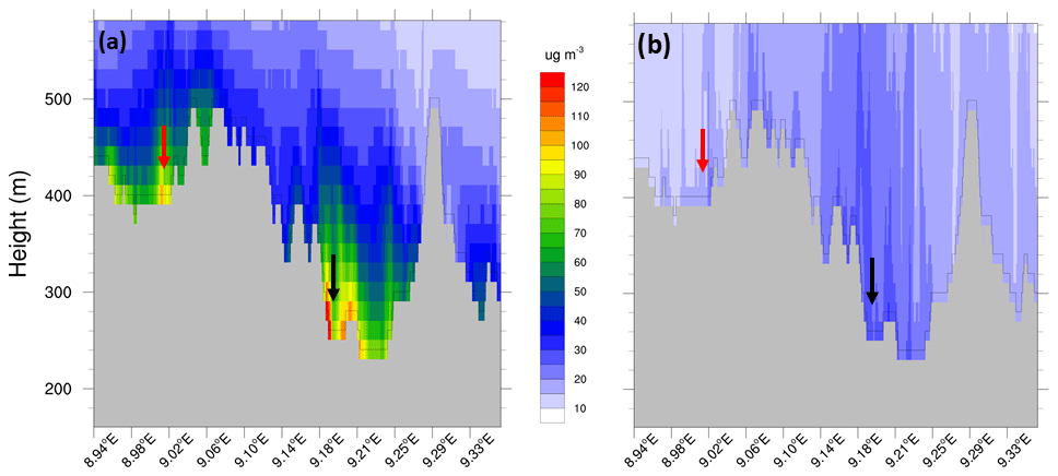
Figure 14 West–east cross section through Neckartor displaying the NO₂ concentration at 07:30 UTC (a) and 12:00 UTC (b) on 21 January 2019. The red arrow denotes the A81 motorway and the black arrow denotes the Neckartor location. The gray area shows the model terrain above mean sea level.

Figure 15 Same as Fig. 14 but for PM₁₀.

4.2.2 Vertical distribution of NO₂ and PM₁₀

In addition to the horizontal distribution of near-surface NO₂ and PM₁₀, TP simulations with a fine vertical resolution also enable qualitative insights into the vertical distribution of pollutants. Figure 14 shows west–east cross sections at Neckartor (Fig. 1b) during the morning rush hour and at noon. Neckartor is one of the heaviest traffic locations in the Stuttgart city area.

The NO₂ concentration during the morning rush hour shows an accumulation along the motorway (red arrow in Fig. 14a) and in the region around Neckartor (white arrow in Fig. 14a), with concentrations exceeding 100 µg m⁻³ as the atmospheric inversion prevents exchange with the layers above (Fig. 7). The vertical extent of concentrations higher than 30 µg m⁻³ is about 200 $\mathrm{m}\mathrm{a}.\mathrm{g}.\mathrm{l}.$ with a strong reduction above.

At noon (Fig. 14b), the simulated NO₂ concentration is much lower (less than 30 µg m⁻³) as turbulence leads to a stronger mixing throughout the boundary layer up to 400 $\mathrm{m}\mathrm{a}.\mathrm{g}.\mathrm{l}.$, which is in accordance with the simulated potential temperature time series shown in Fig. 11.

Figure 15a displays the simulated PM₁₀ concentrations during the morning rush hour. Like for NO₂, higher concentrations of more than 25 µg m⁻³ are simulated along the motorway and in the Stuttgart basin. During the day, PM₁₀ is vertically mixed, showing a clear gradient around 800 $\mathrm{m}\mathrm{a}.\mathrm{s}.\mathrm{l}.$ (Fig. 15b), while concentrations remain between 10–20 µg m⁻³ within the boundary layer.

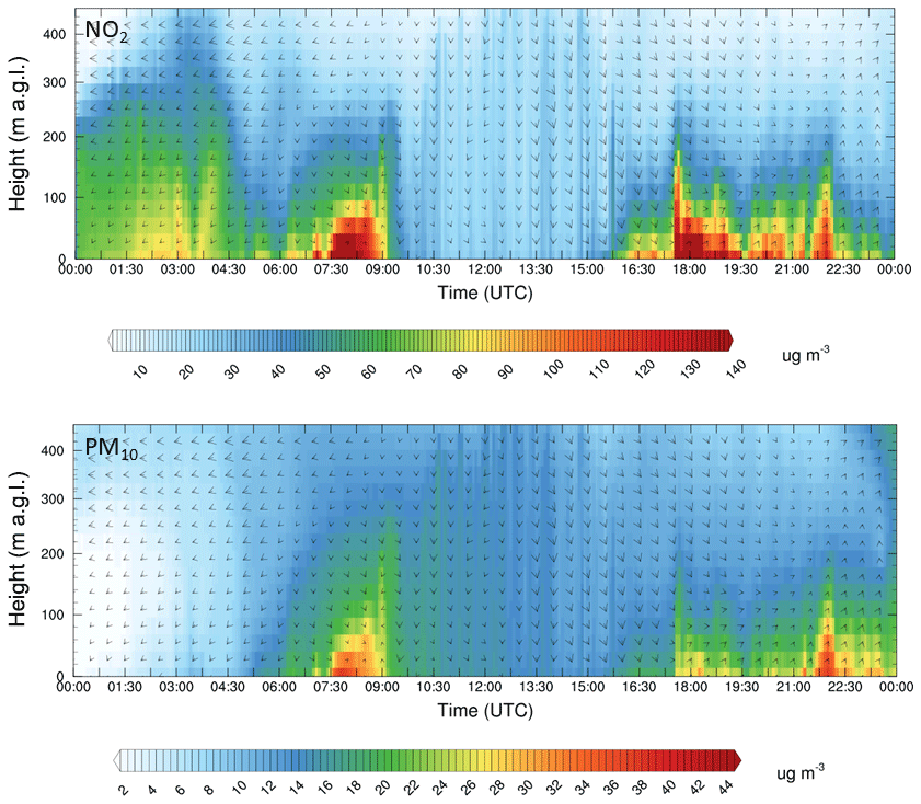
Figure 16 Time–height cross section of NO₂ (top) and PM₁₀ (bottom) at Neckartor (NT) up to an altitude of 450 $\mathrm{m}\mathrm{a}.\mathrm{g}.\mathrm{l}.$

Apart from the west–east cross sections, it is also worthwhile to investigate the vertical temporal evolution of NO₂ and PM₁₀ concentrations. Therefore, Fig. 16 shows time–height cross sections of NO₂ (top) and PM₁₀ (bottom) at Neckartor.

Well visible are the high simulated NO₂ and PM₁₀ concentrations during the morning rush hour, with peak values of more than 120 µg m⁻³ NO₂ and more than 40 µg m⁻³ PM₁₀. The high concentrations of NO₂ and PM₁₀ are present up to around 150–200 $\mathrm{m}\mathrm{a}.\mathrm{g}.\mathrm{l}.$ During daytime, turbulence efficiently mixes the pollutants to higher altitudes, and the near-surface concentrations are quickly reduced. During the evening when the very shallow boundary layer has developed again and evening traffic commences, the particle concentrations increase, and peak values of more than 30 µg m⁻³ are simulated below 100 $\mathrm{m}\mathrm{a}.\mathrm{g}.\mathrm{l}.$

5 Summary and conclusion

This paper describes the setup of an AQFS prototype using WRF-Chem for the Stuttgart metropolitan area. Because of the complex topography in this region, this simulation system requires a very high horizontal resolution down to the TP scale to represent all orographic and land cover features.

For the development of this prototype, 21 January 2019 served as the test case, as this was a typical winter day with an atmospheric inversion. In addition, this day was characterized as “fine dust alarm” situation, where the PM₁₀ concentration at the station Neckartor in the Stuttgart basin was expected to exceed 30 µg m⁻³ (http://www.stadtklima-stuttgart.de/stadtklima_filestorage/download/luft/Feinstaubwerte-2019_AN.pdf, last access: 23 March 2021). The model setup encompassed three domains down to a TP resolution of 50 m.

The initial conditions were provided by the ECMWF operational analysis, the CAMS reanalysis, and WACCM model for background chemistry. Emission data sets from CAMS-REG-AP and high-resolution data with 500 m resolution from LUBW were combined to be used in the AQFS. As current emission data sets only provide annual totals or means, a temporal decomposition following TNO was applied (Denier van der Gon et al., 2011).

For this case study, we focused on the results with respect to 2 m temperature, surface fluxes, and boundary layer evolution as well as horizontal and vertical distributions of NO₂ and PM₁₀.

Our results revealed that despite the complex topography in Stuttgart, the model is in general able to simulate a realistic diurnal cycle of 2 m temperatures, although, compared to observations, differences of up to 1 K occur. Apparently, the model has difficulties with the dissolution of low stratus clouds between 03:00 and 06:00 UTC, which was also reported in the work of Steeneveld et al. (2015), resulting in a warm 2 m temperature bias during the morning. Although no measurements are available, the surface sensible heat fluxes show a clear diurnal cycle with the magnitude clearly depending on the underlying land cover type. The low simulated ground heat flux and its fluctuations between 00:00 UTC and sunrise partially confirm the fog dissolution issue, but more test cases are needed for a more detailed investigation. Over grid cells where the single-layer UCM is active, most of the ground heat flux is stored in the canopy layer thus not transferred into the soil. The high vertical resolution of 100 levels enables a realistic representation of the nocturnal and daytime temperature inversion with an accompanying shallow boundary layer of less than 400 m during the day.

The simulation of PM₁₀ shows an exceedance of the 30 µg m⁻³ concentration threshold close to the Neckartor station and also fulfills the other fine dust alarm criteria shown in Sect. 3. Compared to the usually unevenly distributed air quality measurements, the AQFS allows further insights into the spatiotemporal pollutant distribution. The horizontal distributions of NO₂ and PM₁₀ on this particular day clearly indicate the main polluted areas along the motorways and in the Stuttgart basin. The special orography of Stuttgart with its basin favors the accumulation of NO₂ and PM₁₀ in the morning and evening, while the pollutants are well mixed to around 200–400 $\mathrm{m}\mathrm{a}.\mathrm{g}.\mathrm{l}.$ when the boundary layer is fully evolved.

The simulation also shows that pollutants can be advected from the A81 motorway towards Stuttgart, depending on the wind situation, potentially leading to an increase of the NO₂ and partially PM₁₀ concentrations in the Stuttgart basin. As can be seen from Figs. 12 and 13, the Neckar Valley can also have a large impact on the pollutant concentration in the Stuttgart basin if an atmospheric inversion together with prevailing easterly winds is present.

This is, to our knowledge, the first study of applying WRF-Chem on a TP resolution for an urban area. To derive more robust conclusions with respect to air pollution, more cases studies with different weather situations during winter and summertime are necessary. Nevertheless, our evaluation gives the following indications to further improve the quality of such simulations:

• I.

  applying high-spatial-resolution and high-temporal-resolution gridded emission data from all pollution sources in near-real time to avoid extrapolating annual emissions to individual days (this will help to enhance the simulation of the diurnal cycles of chemical species);

• II.

  improving the chemical background, e.g., by applying higher resolution products from the CAMS European air quality project (Marécal et al., 2015) (this will help to have a more detailed structure of the chemical constituents beneficial for subsequent downscaling simulations);

• III.

  using a longer spin-up period and applying a larger TP model domain to further improve the spin-up of turbulence in the model;

• IV.

  considering vertical distribution of surface emissions (e.g., Bieser et al., 2011; Guevara et al., 2021);

• V.

  considerably increasing the number of pollutant measurements to allow more robust conclusions.

The AQFS has a great potential for urban planning applications. For example, land cover could be changed from urban low density to urban high density to investigate the impact of urban re-densification, e.g., on temperature and air quality. Although no BEP can be applied on the TP resolution with our combination of parameterizations, changes of the parameters required for the single-layer UCM offer the opportunity to perform sensitivity analysis with respect to different building heights, urban greening effects (Fallmann et al., 2016), or anthropogenic heating (Karlický et al., 2020). Recently, Lin et al. (2020) developed an interface to use output from high-resolution WRF simulations to force PALM 6.0 in an offline mode, which could be another tool in the future to study microscale structures in urban areas.

In the future, more emphasis should also be put on an improvement of the I/O (e.g., by means of quilting) and additional OpenMP capabilities in WRF-Chem. However, simulations with WRF-Chem at the TP resolution will still require around 1500–2000 compute cores for operational use due to the small numerical time step necessary.

Although air quality modeling on the TP scale is a very challenging and a computationally expensive task, we are convinced that the AQFS will have great potential to further improve process understanding and will certainly help politicians make decisions on a more scientifically valid basis.