the Creative Commons Attribution 4.0 License.
the Creative Commons Attribution 4.0 License.
 | 22 Mar 2021
Drivers of the fungal spore bioaerosol budget: observational analysis and global modeling
Allison L. Steiner
Anne E. Perring
J. Alex Huffman
Ellis S. Robinson
Cynthia H. Twohy
Luke D. Ziemba
Bioaerosols are produced by biological processes and directly emitted into the atmosphere, where they contribute to ice nucleation and the formation of precipitation. Previous studies have suggested that fungal spores constitute a substantial portion of the atmospheric bioaerosol budget. However, our understanding of what controls the emission and burden of fungal spores on the global scale is limited. Here, we use a previously unexplored source of fungal spore count data from the American Academy of Allergy, Asthma, and Immunology (AAAAI) to gain insight into the drivers of their emissions. First, we derive emissions from observed concentrations at 66 stations by applying the boundary layer equilibrium assumption. We estimate an annual mean emission of 62 ± 31 m−2 s−1 across the USA. Based on these pseudo-observed emissions, we derive two models for fungal spore emissions at seasonal scales: a statistical model, which links fungal spore emissions to meteorological variables that show similar seasonal cycles (2 m specific humidity, leaf area index and friction velocity), and a population model, which describes the growth of fungi and the emission of their spores as a biological process that is driven by temperature and biomass density. Both models show better skill at reproducing the seasonal cycle in fungal spore emissions at the AAAAI stations than the model previously developed by Heald and Spracklen (2009) (referred to as HS09). We implement all three emissions models in the chemical transport model GEOS-Chem to evaluate global emissions and burden of fungal spore bioaerosol. We estimate annual global emissions of 3.7 and 3.4 Tg yr−1 for the statistical model and the population model, respectively, which is about an order of magnitude lower than the HS09 model. The global burden of the statistical and the population model is similarly an order of magnitude lower than that of the HS09 model. A comparison with independent datasets shows that the new models reproduce the seasonal cycle of fluorescent biological aerosol particle (FBAP) concentrations at two locations in Europe somewhat better than the HS09 model, although a quantitative comparison is hindered by the ambiguity in interpreting measurements of fluorescent particles. Observed vertical profiles of FBAP show that the convective transport of spores over source regions is captured well by GEOS-Chem, irrespective of which emission scheme is used. However, over the North Atlantic, far from significant spore sources, the model does not reproduce the vertical profiles. This points to the need for further exploration of the transport, cloud processing and wet removal of spores. In addition, more long-term observational datasets are needed to assess whether drivers of seasonal fungal spore emissions are similar across continents and biomes.
- Article
(10755 KB) - Full-text XML
-
Supplement
(866 KB) - BibTeX
- EndNote


Bioaerosols are omnipresent in the global atmosphere (DeLeon-Rodriguez et al., 2013; Després et al., 2012; Fröhlich-Nowoisky et al., 2016). They contribute to the organic aerosol burden of the atmosphere and therefore can affect weather and climate by influencing cloud and precipitation formation. They can act as ice-nucleating particles (INPs; Haga et al., 2014; Pratt et al., 2009; Tobo et al., 2013; Twohy et al., 2016) and can form cloud condensation nuclei (CCN) upon fragmentation in the atmosphere (China et al., 2016; Steiner et al., 2015). Furthermore, bioaerosols can have adverse impacts on human health by acting as pathogens, allergens or toxins (Fröhlich-Nowoisky et al., 2016; Reinmuth-Selzle et al., 2017; Samake et al., 2017) and play a role in the transmission of crop and animal pests (Fisher et al., 2012).
Bioaerosols include bacteria, fungal spore, pollen and fragments of other organisms, such as plants. The first three groups all include species that can act as CCN or INPs (Fröhlich-Nowoisky et al., 2016), although their activities as cloud nuclei differs per species. The significance of bioaerosol for cloud formation on global and regional scales depends on their abundance, and their relative contribution to INP and CCN populations compared to other aerosol types. On the global scale, their contribution to ice crystal formation is thought to be limited (Hoose et al., 2010; Spracklen and Heald, 2014), although they could still be of importance for cloud formation in specific regions, such as the Amazon (China et al., 2016, 2018; Morris et al., 2014; Pöschl et al., 2010; Prenni et al., 2009).
Estimates of the emissions of bioaerosols on the global scale vary over almost 2 orders of magnitude, which prohibits accurate assessment of their impact on cloud formation and air quality. An early estimate that was based on extrapolation of measurements at a few locations was as high as 1000 Tg yr−1 (Jaenicke, 2005). Subsequently, global model simulations have been performed that included parameterizations for three main classes of bioaerosols (i.e., pollen, fungal spores and bacteria). These yielded total emission estimates between 62 and 123 Tg yr−1 (Hoose et al., 2010; Myriokefalitakis et al., 2017), with variations between models due to differences in meteorology and land use maps. The variation of estimates for the global bioaerosol burden is large as well, ranging between 121 and 791 Gg and resulting from differences between models in emissions, assumed size distributions and formulation of removal mechanisms. However, the emission parameterizations that are incorporated in these models are based on limited observations. All of the above studies used the same emission schemes, or modified versions thereof. The fungal spore emission scheme of Heald and Spracklen (2009), referred to as HS09 hereafter, is based on measured concentrations of mannitol, a sugar alcohol that is a proxy for fungal spore concentrations, at a limited number of locations, and simulated emissions of fine and coarse spores from all ecosystems as a function of LAI and specific humidity. Note that Myriokefalitakis et al. (2017) used a modified form of the HS09 scheme, based on Hummel et al. (2015). An early pollen emission scheme (Jacobson and Streets, 2009) was not based on, or tested against, observations. More recently, pollen emission schemes have been developed based on pollen count observations and implemented in regional-scale models (Wozniak and Steiner, 2017; Zink et al., 2013). Finally, the bacteria emission scheme by Burrows et al. (2009) was developed by inverse modeling of measured bacteria concentrations over various ecosystems and assumes constant emissions for each land use type. Since estimates of the global bioaerosol burden strongly depend on their emissions, emission models that are better constrained by observations are urgently needed.
In this work, we focus on fungal spores, as they have a smaller size than pollen, which implies that they are more likely to be transported over longer distances, and to contribute significantly to the organic aerosol budget on the regional and global scale. They can also produce large quantities of submicrometer fragments after rupturing in the atmosphere and thereby contribute to CCN and INP populations (China et al., 2016; O'Sullivan et al., 2015). Fungi emit spores into the air as part of their reproductive strategy. These emissions are thought to depend on temperature and water availability (Boddy et al., 2014; Gange et al., 2007; Jones and Harrison, 2004; Löbs et al., 2020), along with biotic factors. Emissions of spores into the atmosphere can be either active or passive, depending on the species of fungus. Active emission mechanisms include emissions at high relative humidity with liquid jets or droplets (Elbert et al., 2007; Pringle et al., 2005). Factors that have been proposed to drive the passive emission of fungal spores into the atmosphere include wind (Jones and Harrison, 2004) and rainfall (Huffman et al., 2013; Prenni et al., 2013). Since the sources of fungal spores are diverse, it is challenging to develop a mechanistic description of their atmospheric emissions, and therefore emissions are usually based on extrapolation of the limited number of available observations. These estimated emissions of fungal spores range widely for different methods, including both models and educated guesses, from 50 Tg yr−1 (Elbert et al., 2007), 28 Tg yr−1 (HS09), 186 Tg yr−1 (Jacobson and Streets, 2009) to 79 Tg yr−1 (Sesartic and Dallafior, 2011). Moreover, the seasonal cycle in these estimates is either absent or assumed to be instantaneously related to the seasonal cycle of the driving variables.
In this study, we develop two new schemes for the emission of fungal spores on seasonal timescales (Sect. 2), using a previously unexplored source of observed fungal spore concentrations over the United States and building on available knowledge about the drivers of their emissions. Subsequently in Sect. 3, we implement these new emission schemes in the GEOS-Chem chemical transport model (Sect. 3.1) to calculate the global emissions and burden of fungal spores (Sect. 3.3). Finally, we evaluate the ability of both emission schemes to simulate spatial and seasonal variations in observed fungal spore concentrations and compare results from the new schemes to those from the previously developed Heald and Spracklen (2009) scheme (Sect. 3.4).
In this section, we first describe how we infer fungal spore emissions from observed concentrations, and subsequently we explain how we develop two new emission parameterizations from these derived emissions. The first parameterization is a purely statistical one and is derived by relating spore emissions to meteorological and land use variables, using multivariate linear regression. The second parameterization is based on the fact that fungal spore production is the result of a biological process. We aim to represent the production of spores with a simple population model that accounts for the growth of fungi and fungal spores during the year. The overall goal is to obtain emission models that are better constrained and validated by observational data than the existing HS09 model but that are still simple and straightforward to implement in 3D models.
2.1 Fungal spore observations
Our emission scheme is based on multi-annual time series (6 years, from 2003 to 2008) of spore counts at 66 stations across the continental USA operated by the American Academy of Allergy, Asthma, and Immunology (AAAAI). Members of the National Allergy Bureau monitor spore and pollen counts at these stations, where samples are collected on at least 3 d a week using a Burkard spore trap (Hirst, 1952; Levetin, 2004). Spore traps are situated on an unobstructed rooftop at least one story above ground (http://pollen.aaaai.org/nab, last access: 7 June 2020). In the Burkard spore trap, air is drawn into a 14 mm × 2 mm orifice at 10 L min−1, and any airborne particles with sufficient inertia are impacted on either a greased tape or a greased microscope slide beneath the orifice. The slides are then examined by microscopy for counting and identification of spores. The standard orifice on the Burkard sampler is efficient for particles down to 3.7 µm (Levetin, 2004), which means that the collection efficiency of the smallest spores is less than unity. The reported spore counts therefore represent lower limit values: for the size distribution parameters as defined in Sect. 3.2, ∼ 40 % of the mass concentration and ∼ 83 % of the number concentration would fall in the size range for which the collection efficiency is below unity. Without a better understanding of how the collection efficiency varies with size, we cannot assess what fraction of these particles go undetected by the Burkard spore trap.
Specified spore counts are available at the genus level, but for our analysis we only use the total daily spore counts. The observed concentration ranges between 0 and 6.3×10⁴ m−3 for all stations and years with a mean of 5.4×10³ m−3. Figure 1 shows a map with an overview of the AAAAI stations used in this analysis (with the exception of Anchorage, AK), and the mean spore concentration over the full length of the measurement period for each station. For 36 % of the stations, no observations were available during winter, which has consequences for the derived fluxes during that time of year (see Sect. 3.1). The map also shows the land use, which is a simplified version of the Olson terrestrial ecoregions dataset (Olson et al., 2001), and uses the same lumping into broad land use categories as Burrows et al. (2009). The concentrations show no clear relation to land use types, although the three stations with the lowest concentrations are located in regions that are dominated by deserts and shrubs.
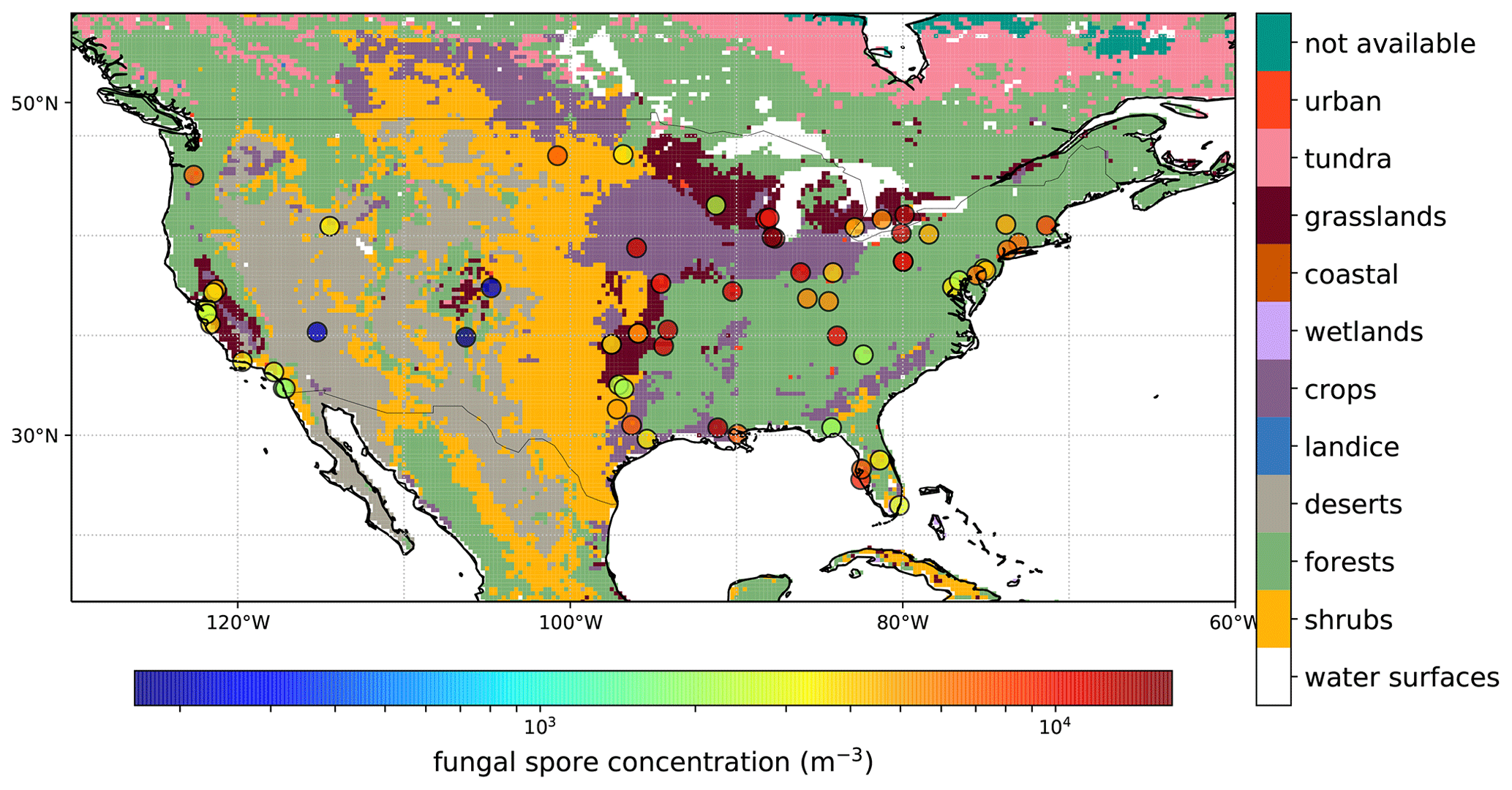
Figure 1Average observed fungal spore concentrations over the period 2003–2008 for all AAAAI stations (circles) shown on top of lumped land use classes bases on the Olson World Ecosystems (Olson et al., 2001).
2.2 From concentrations to fluxes
To develop an emission scheme from these observations, emission fluxes need to be derived from measured concentrations first. This derivation consists of two steps: (1) the conversion from concentrations to net surface fluxes and (2) the conversion from net surface fluxes to emissions fluxes, by subtracting the deposition flux. We describe this procedure here, using Fig. 2 to visually present an example at one site.
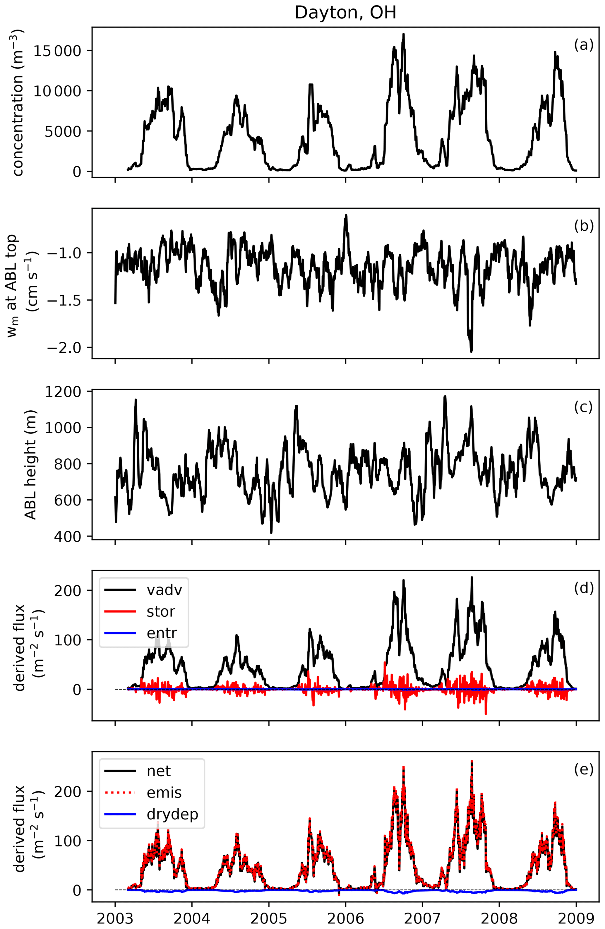
Figure 2Example of how emissions flux is derived from observed concentrations at one AAAAI site located in Dayton, OH. Shown here are 20 d running mean time series of (a) fungal spore concentration; (b) subsidence velocity at atmospheric boundary layer (ABL) top; (c) mean height of the afternoon boundary layer; (d) contributions of vertical advection (vadv), storage (stor) and entrainment (entr) terms to the calculated flux; and (e) calculated net flux, emission flux and dry deposition flux.
Rainfall poses a challenge for deriving bioaerosol fluxes. A number of studies (e.g., Geagea et al., 2000; Huffman et al., 2013; Prenni et al., 2013) have demonstrated that rain can act as a trigger for the release of bioaerosols from vegetation and soils. However, at the same time, wet deposition removes aerosols from the atmosphere. This offsetting effect complicates the relationship between rainfall and net fungal spore fluxes. Therefore, to simplify our analysis, we remove spore counts from our observational dataset that were made on days on which any rainfall occurred (on average 32 % of the days at each station), as established by the categorical rain (crain) variable in the National Centers for Environmental Prediction (NCEP) North American Regional Reanalysis (NARR) product (Mesinger et al., 2006) dataset. This necessarily prohibits an assessment of the influence of rainfall on fungal spore emissions on the same day. We note that this is a coarse filtering and that emissions of fungal spores may respond to rainfall on timescales of up to 3 d (Sarda-Estève et al., 2019). Given our focus on 20 d average emissions (see below), we do not apply a more sophisticated treatment, but note that further efforts to characterize the relationship between fungal spore emissions and rainfall could inform higher temporal resolution modeling.
There are several methods available for translating atmospheric concentrations to surface fluxes. Here, we apply the equilibrium boundary layer assumption (Betts, 2000), which states that over sufficiently long periods (at least several days), boundary layer depth over land reflects a statistical equilibrium between surface heating that acts to deepen the boundary layer and subsidence of free-tropospheric air that acts to decrease boundary layer height. The surface flux can then be calculated from boundary layer concentrations by applying the tracer conservation equation, which accounts for the effects of horizontal and vertical transport. We assume that convection maintains a well-mixed boundary layer, in which scalars, reactants and aerosols have a constant profile over the depth of the boundary layer. This method has been used before to infer seasonal CO2 surface fluxes from measured concentrations (Bakwin et al., 2004; Helliker et al., 2004). We have to note here that it is hard to assess the validity of the assumption of well-mixed profiles of fungal spores in the boundary layer, since only limited observations of vertical profiles throughout the boundary layer are available. Observations show that concentrations of spores are actually highest in the surface layer (Perring et al., 2015), where the AAAAI measurements are taken. Taking these concentrations as representative of boundary layer values means that we overestimate their emission fluxes. Calculated emissions in this work should therefore be regarded as upper limit values. We explore the sensitivity of these emissions to assumptions on vertical mixing parameters in Sect. 4.
The tracer conservation equation in a simplified form, which does not account for horizontal advection, is as follows:
in which Fs is the surface flux (m−2 s−1), 〈C〉 is the boundary layer concentration of species C (m−3), CFT is the free-tropospheric concentration of C (m−3), wm is the subsidence velocity at boundary layer top (m s−1), h is the well-mixed boundary layer height (m), and t is time. The three terms on the right-hand side of Eq. (1) represent the vertical advection, storage and entrainment terms, respectively.
In our analysis, C is the concentration of fungal spores in the boundary layer as reported at the AAAAI stations. The measurement heights for the AAAAI stations are not specified, but the measurement locations are at least one story above the ground. This means that the sampling locations are in the atmospheric surface layer, which likely leads to an overestimation of the boundary layer concentrations. For instance, Perring et al. (2015) found that PBAP concentrations aloft (up to the 900 hPa level) are only between 5 %–55 % of those at the surface. The concentration of fungal spores in the free troposphere (CFT) is not well characterized. Based on the vertical profile of fluorescent bioaerosol concentrations observed in and above the boundary layer over the US western plains (Twohy et al., 2016), we assume that the concentration of spores decreases by about an order of magnitude between boundary layer (BL) and free troposphere (FT). Hence, we set CFT=0.1〈C〉. This is clearly a crude assumption and we discuss the sensitivity of the calculated fluxes to different values of this dilution factor in Sect. 5.
We take the subsidence velocity from the NARR data, as vertical velocity interpolated to the mean height of the afternoon (12:00–18:00 local time) boundary layer top (Fig. 2b). With a spatial resolution of 32 km (about 0.3∘) and 8 output fields per day (representing 3-hourly averages), NARR output provides a reasonable spatial and temporal match for each of the AAAAI stations of interest. In the boundary layer equilibrium assumption, we take the mean height of the afternoon boundary layer from NARR as the daily boundary layer height (Fig. 2c). We assume that the height of the mixed-layer during daytime is representative of the mean boundary layer height for each day, and that the summed depth of the nocturnal boundary layer and the residual layer during nighttime is similar to the daytime boundary layer height (Bakwin et al., 2004; Helliker et al., 2004).
Williams et al. (2011) found that for CO2, horizontal advection can be of the same order of magnitude as vertical advection. For fungal spore concentrations, the horizontal heterogeneity is likely stronger than for a long-lived tracer like CO2, due to the short atmospheric lifetime of these coarse particles and the heterogeneity of their sources. Therefore, horizontal advection possibly has a large influence on spore concentrations. By applying running averages over a period of 20 d, we aim to average out some of this horizontal variability, while acknowledging that this implicitly assumes long-term horizontal homogeneity, which may not be realistic for every AAAAI station. In Eq. (1), horizontal advection is neglected, because there is no reliable way to constrain the horizontal transport of fungal spores.
We use Eq. (1) to calculate running average fluxes over 20 d in order to minimize the effects of synoptic-scale variability on the relationship between concentration and flux while maintaining the seasonal cycle (Bakwin et al., 2004). A consequence of this choice is that the contribution of short-term storage and entrainment effects to the calculated surface flux is minimal (Williams et al., 2011). Figure 2d shows the calculation of the three terms from Eq. (1). The vertical advection term contributes most to the calculated net surface flux, and therefore we explore how assumptions related to this term impact derived fluxes in Sect. 3.4. In contrast, the combined storage+entrainment term becomes negligible in magnitude (< 10 %) compared to the surface flux for most stations when an averaging period of 20 d is applied (Fig. S1 in the Supplement), which shows that at seasonal timescales storage and entrainment contributions can be neglected without introducing large errors in the surface flux calculation. Whether inclusion of horizontal advection in the boundary layer budget equation would substantially impact these results remains an open question. It likely varies per site, depending on whether there are spore sources upwind of the site or not.
As a final step in the derivation of the emission flux of fungal spores, we calculate the dry deposition flux with an offline version of the aerosol dry deposition scheme that is also used in the GEOS-Chem model (Zhang et al., 2001). To run this bulk deposition scheme, we use meteorological fields from the NARR as input and we assume a mean fungal spore diameter of 2.5 µm (see Sect. 3.2) and a density of 1 g cm−3 (Heald and Spracklen, 2009). The calculated deposition velocities are low (< 0.1 cm s−1) at all stations and seasons, so the deposition flux is of minor influence in the derivation of the emission flux from the net surface flux (Fig. 2e).
The conversion of the fungal spore counts to emission fluxes yields a mean emission of 62 ± 31 m−2 s−1 over all years and stations, with a strong seasonal cycle. The mean ratio between concentrations and fluxes does not vary substantially between sites and land use types (Fig. S2). About a third of the stations (26) are associated with the “forests” land use type, while other land use types are not as well represented in the dataset (Fig. 1). Therefore, for the purpose of developing the emission scheme, we do not distinguish between land use types. Very few flux measurements of bioaerosols in general and fungal spores in particular are available to compare the magnitude of emission that we estimate here. Carotenuto et al. (2017) measured microbial fluxes over a Mediterranean grassland, reporting mean fluxes of 8.3 ± 11.1 m−2 s−1 in 2008–2010 and 10.6 ± 6.2 m−2 s−1 in 2015. However, comparison with our derived fluxes is complicated by the fact that they report net fluxes of viable bioaerosols, which represent only a fraction of the total bioaerosol population and are likely composed of both fungal spores and bacteria. Crawford et al. (2014) derived fluorescent bioaerosol fluxes over a Colorado pine forest by applying flux–gradient relationships. Fluorescent clusters that were tentatively associated with fungal spores showed estimated nighttime emissions up to 6000 m−2 s−1 under humid conditions, although they observed net deposition fluxes during much of the rest of the day and under dry conditions. Finally, Ahlm et al. (2010) reported upward fluxes of accumulation-mode particles in a tropical forest of up to 5000 m−2 s−1. They claim that these emitted particles could be fungal spores, although their observations are complicated by dry deposition of particles of supposedly anthropogenic origin. More definitive measurements of spore fluxes would be useful for further comparison with our derived fluxes.
2.3 Statistical model for spore emissions
For our initial model, we take a purely statistical approach in quantifying fungal spore emissions at seasonal timescales and perform a multivariate linear regression (MLR) on the derived fungal spore fluxes. For this purpose, we combine the AAAAI data with MERRA2 meteorological data (Gelaro et al., 2017) at resolution. With our objective of implementing this emission scheme into the GEOS-Chem model, we use MERRA2 meteorology here (as used in GEOS-Chem), rather than the NARR dataset used in Sect. 2.2. In addition, the NARR archive does not contain some surface variables that are relevant for describing land-surface–atmosphere exchange, such as friction velocity and roughness length. For the most important variables in our analysis (temperature at 2 m (T2 m) and specific moisture at 2 m (q2 m)), we verify that the MERRA2 and NARR datasets are consistent. We find very good agreement between the two datasets despite different origins and spatial resolutions, with r2=0.94 and NMB = 0.0 for T2 m and r2=0.92 and NMB =0.03 for q2 m. For wind speed at 10 m (U10 m), we do not find good agreement (r2=0.01 and NMB .59), but this variable is less important in our analysis than T2 m and q2 m. Therefore, we conclude that the choice of meteorological dataset does not have a major impact on our analysis.
In addition to MERRA2 data, we use 4 d LAI observations from MODIS (Myneni et al., 2015) aggregated to resolution as a variable in our regression analysis. The LAI data used here show good agreement with the LAI used in the GEOS-Chem simulations, with r2=0.80 and NMB .02. We also include time (measured in days from the start of the AAAAI time series) to account for any linear trend in fungal spore emissions, as in Porter et al. (2015). Variables showing a strongly skewed distribution (e.g LAI and 2 m temperature) were log-transformed to fulfill the MLR requirement of normally distributed variables.
In the MLR, the first independent variable is selected based on the r2 score. Subsequently, all other variables are tested and the one that leads to the largest decrease in the Bayesian information criterion (BIC) is kept as a second independent variable.
This procedure is repeated until all meteorological and land surface variables are evaluated. Finally, we only keep the variables that lead to a significant decrease in BIC for inclusion in the statistical model. The BIC provides a measure of relative model performance and can be used to find an optimum number of explanatory variables in statistical models, by including a penalty for overfitting (Porter et al., 2015). Unlike the r2, it will not increase whenever a new variable is added but rather yields a minimum value at which a maximum model skill is reached without including redundant variables.
The regression analysis identifies specific humidity at 2 m (q2 m), leaf area index (LAI) and friction velocity (u∗) as the top independent variables that explain the seasonal cycle in fungal spore emissions (Fig. 3). Figure 3 shows that a minimum in ΔBIC is not reached until after the inclusion of about 6 variables. Given that including this many variables is somewhat impractical and the gain in model skill (represented by r2) by adding additional variables is small, we choose to limit the number of predictors to three. Several independent variables have similar correlations with the spore emissions; therefore we have tested the robustness of our variable selection method by forcing different variables as the first variable in the MLR analysis (LAI and 2 m temperature T2 m). In each of these cases, the top three independent variables are a combination of q2 m, LAI, u∗ and T2 m, which gives confidence in the selection of q2 m, LAI and u∗ as driving variables in our statistical model. Our statistical emission function is thus
with coefficients b0–b3 as in Table 1 (determined from fitting procedure described in Sect. 2.5).
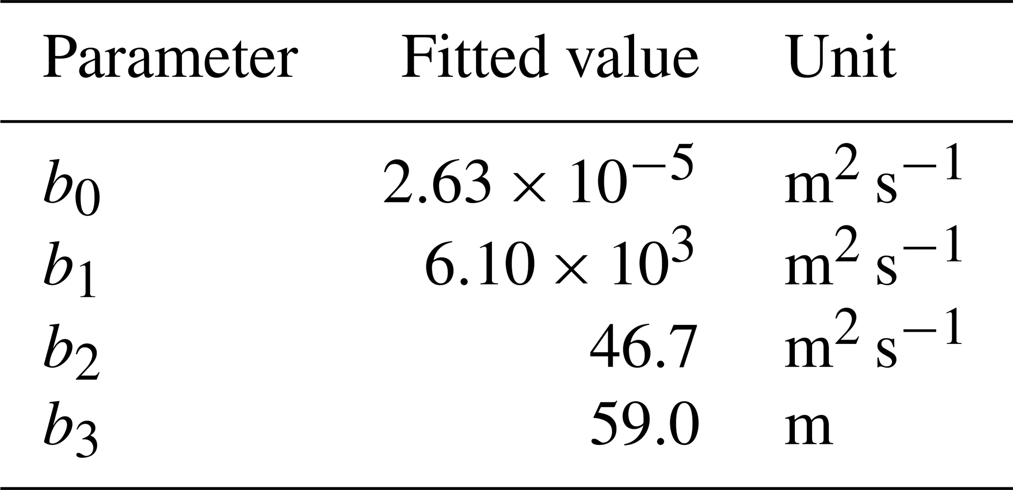
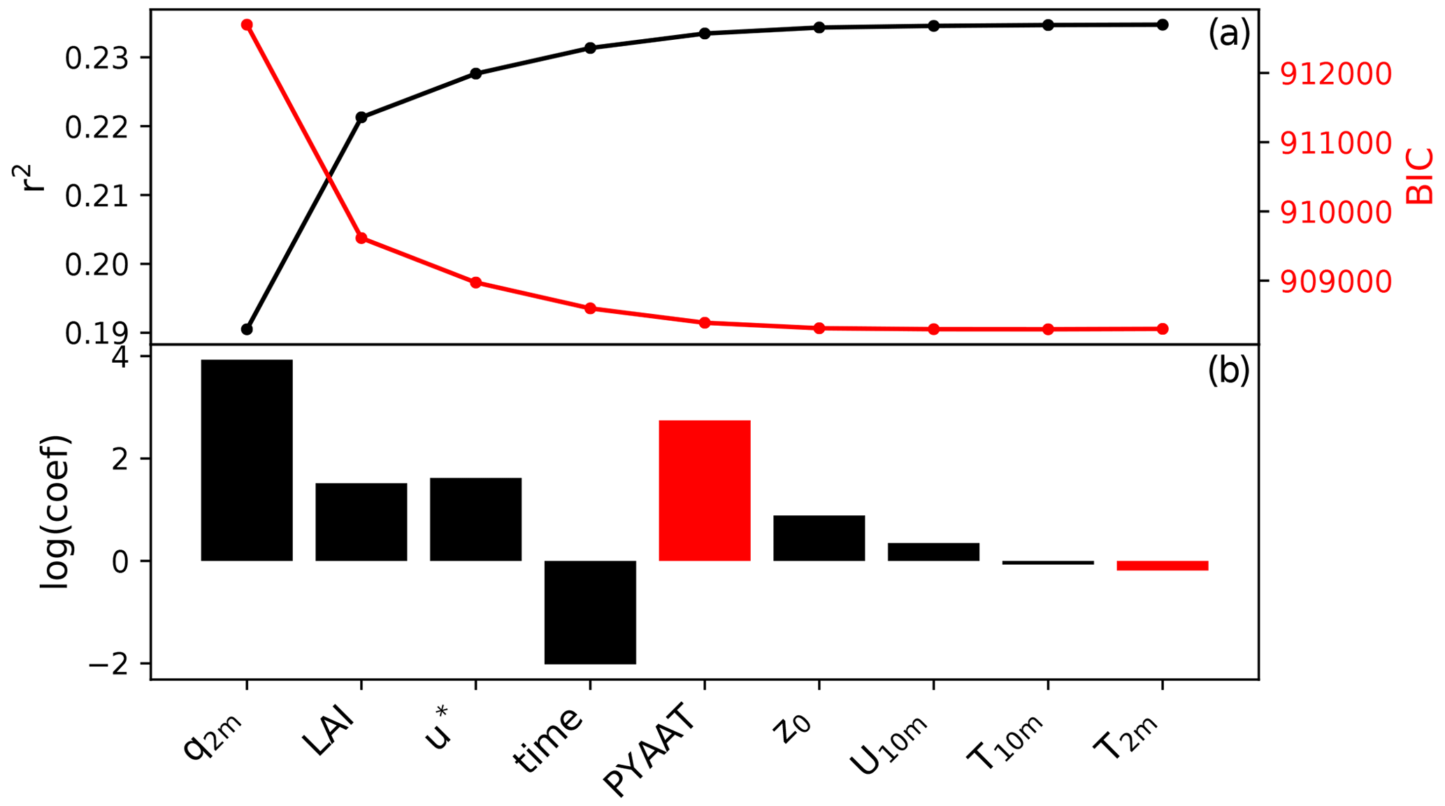
Figure 3Results of the multivariate regression analysis: r2 and BIC after including each variable in the MLR analysis (a) and the logarithm of the regression coefficient for each variable (b). Red bars indicate a negative regression coefficient. The variables included are specific humidity at 2 m (q2 m), leaf area index (LAI), friction velocity (u*), time (expressed as number of days since start of time series), previous year annual average temperature (PYAAT), roughness length (z0), temperature at 2 m (T2 m), wind speed at 10 m (U10 m) and temperature at 10 m (T10 m).
This selection does not mean that the chosen variables specific humidity, LAI and friction velocity are in fact the actual drivers of fungal spore emissions on seasonal timescales. Rather, they are variables which show a similar seasonal cycle to, and therefore a statistical relationship with, the emissions over all stations and years. Therefore, they can be tentatively associated with the growth of fungi and the emission of spores. In other words, it seems likely that humidity and vegetation biomass in some form play a role in the growth of fungi and wind speed in the emission of their spores, and it is therefore plausible that the correlations are indicative of the actual underlying mechanisms. Note that the first two variables are the same as identified in the previous fungal spore scheme developed by HS09. Furthermore, we note that other meteorological drivers, including rain which is specifically excluded here, may become important for controlling fungal spore emissions at shorter timescales.
2.4 Population model for spore emissions
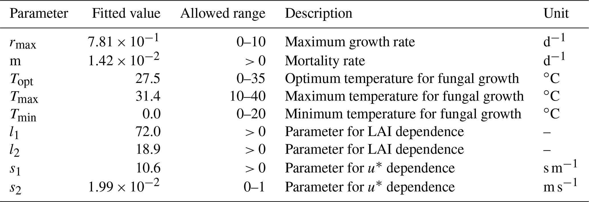
A model that explains and quantifies the emissions of fungal spores at the seasonal timescale should contain the driving variables of spore emissions at the appropriate timescale. These drivers may include both environmental and biological factors. In the literature on fungal growth, temperature and moisture are often mentioned as environmental factors that determine fungal fruiting patterns (Boddy et al., 2014; Damialis et al., 2015; Gange et al., 2007; Kauserud et al., 2008), while resource availability and competition are also thought to play a role.
Here, we take a first-order approach and assume that fungal fruiting (and subsequent spore production) is a biological process that is temperature driven. Further, we assume that greater vegetation biomass can sustain larger fungal populations, by providing more resources for fungi to thrive on. Hence, we represent fungal growth by a logistic growth model, in which the growth rate is a function of temperature and the carrying capacity a function of LAI:
in which N is the population size (m−2), r the growth rate (s−1), K the carrying capacity (m−2) and m the mortality rate (s−1). The mortality term is added to ensure that the fungal population decays when conditions are not suited for growth. The growth rate is represented as follows:
in which rmax is the maximum growth rate (s−1); Tmax, Tmin and Topt are the maximum, minimum and optimal temperatures for fungal growth (∘C), respectively; and T is the actual temperature (∘C).
The carrying capacity K is assumed to be a linear function of LAI:
in which l1 and l2 (m−2) are two fitting parameters that determine the sensitivity of K to LAI.
Emissions of spores from the fungi are then modeled as a function of friction velocity, following a saturation function (Carotenuto et al., 2017; Zink et al., 2013):
in which fu∗ is a dimensionless emission factor which is a function of friction velocity u∗ (m s−1), and in which s1 and s2 are two fitting parameters that determine the sensitivity of to u∗.
Finally, the emission flux of fungal spores Fpop (m−2 s−1) is calculated as follows:
An important simplification in this model is the fact that we do not make any distinction between the population size of the fungi and the number of spores that they produce. In principle, this distinction could easily be included in this formulation by separating the number of fungi and fungal spores into two variables in Eq. (3). However, we have no observational constraints on the size and number of fungi, and therefore such a distinction would only increase the number of variables and free parameters in the set of equations, without providing any verifiable results for the fungal population size. An implicit assumption in this model, which is a consequence of not explicitly including a reservoir of spores, is that emissions have no effect on the fungal spore population size.
2.5 Model fitting
We fit the statistical model, the population model and the HS09 model to the mean calculated emission time series over all stations (Fig. 4), using a non-linear least-squares minimization algorithm (Newville et al., 2014). Meteorological fields from MERRA2 were used in this fitting procedure to ensure consistency with the meteorological data that are used to drive atmospheric transport in GEOS-Chem. When we fit the statistical model with q2 m, LAI and u∗ as independent variables to the emission time series, we find that it has reasonable skill in explaining the seasonality of the observation-based emissions, with r2=0.74 and NMB .004 (Fig. 4a). Table 1 shows the parameter values for the best fit. The fitted population model captures the seasonal cycle in fungal spore emissions better than the statistical model with r2=0.85 and NMB =0.004. Table 2 shows the fitted parameters for the population model. In essence, spore emissions in the population model follow a delayed response to temperature and LAI, due to the growth and mortality of the fungi. The friction velocity has only a minor influence on the emissions. Of the three models, the HS09 model, which shares two variables with the statistical model but has only one regression coefficient (i.e., it is of the form ), shows the least skill in representing the timing and magnitude of the seasonal cycle (r2=0.72 and NMB .193). The fitted coefficient c here has a value of gC m2 s−1 (4.4×10³ m−2 s−1), which is substantially lower than the original value of gC m−2 s−1 for the fine mode in HS09. We note that the original HS09 scheme was derived using a much more limited set of mannitol observations. These mannitol observations (which are an indirect constraint on spore counts) were taken from a handful of sites around the world and did not have the fully resolved seasonal cycle that the AAAAI observations have, and these differences and uncertainties result in a difference of a factor of 2 when fitting HS09. Both the statistical and the HS09 model predict a seasonal cycle which is out of phase with the derived emissions by roughly 1 to 2 months (Fig. 4). Some years show two peaks in derived spore emissions (for instance, there are peaks in June and August–September 2005, and in June and September–October 2008), which are not reproduced by any of the models.
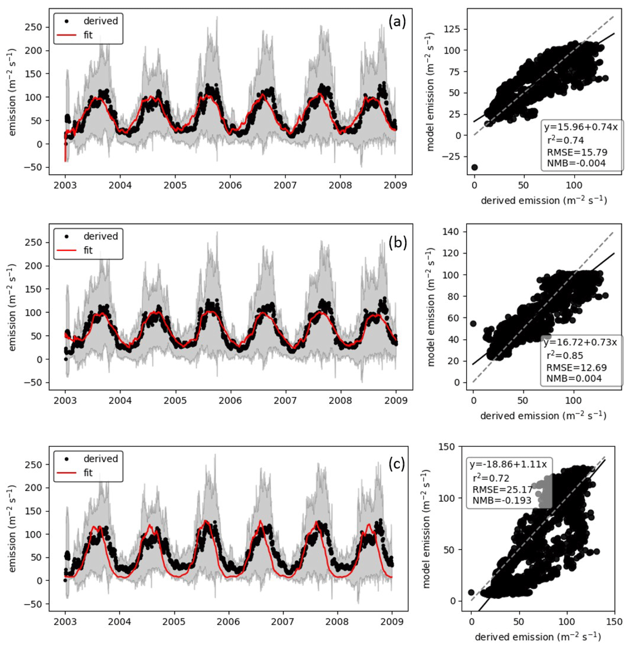
Figure 4Model fungal spore emissions for the (a) statistical scheme, (b) population scheme and (c) HS09 scheme compared to the 20 d running mean derived emission flux at all 66 AAAAI stations. Left panels show time series comparisons over 6 years; shaded areas show the standard deviation of the derived fluxes. Right panels show point-by-point comparison with statistics shown inset and the 1:1 line shown as a dashed line.
3.1 Chemical transport model
We implement our newly developed fungal spore emission schemes in the GEOS-Chem chemical transport model (v11-01; https://www.geos-chem.org, last access: 7 June 2020). Simulations are run for two years (2015 and 2016), of which the first year is used for spin-up, with an emission and transport time step of 30 and 10 min, respectively. The model is driven by assimilated meteorology from the NASA Global Modeling and Assimilation Office (GMAO), here using the MERRA2 product (Gelaro et al., 2017). Global simulations are performed at a horizontal resolution of 2∘ × 2.5∘ and 47 vertical levels. Spore emissions are implemented as a Harvard–NASA Emission Component (HEMCO; Keller et al., 2014) extension, which uses the model meteorology at either the surface or the lowest vertical level, and MODIS LAI product from Yuan et al. (2011) for the year 2008 to calculate emissions (note that the MODIS product used here is not available for 2016, but we find only a minor difference in LAI between 2008 and 2016 in an offline comparison and therefore do not expect this to noticeably impact results shown here).
The dry deposition and sedimentation of aerosol particles is described by the Zhang et al. (2001) bulk aerosol deposition scheme. We made minor adaptations to this scheme to accommodate sedimentation of bioaerosols as a new coarse aerosol class, in addition to dust and sea salt. The mean diameter of the assumed size distribution for the different schemes is applied in the dry deposition calculations (see Sect. 3.2 for a discussion of assumed particle size). Wet deposition is treated by the Liu et al. (2001) scheme, assuming that spores are in the coarse mode. In this scheme, we assume efficient scavenging of fungal spores by rainout and conversion of cloud condensate to precipitation. We address the validity of this assumption in a sensitivity analysis (see Sect. 5).
In our initial simulations, we found unrealistically high fungal spore concentrations in winter for several locations in the USA and Europe in our new schemes (see Sect. 3.5). This is the result of the interplay between low but steady emissions in winter and (a lack of) wet deposition for the simulated year. Since the AAAAI data show gaps for many stations in winter and our observational analysis does not explicitly take into account wet removal, it is likely that our emission schemes are not representative of winter conditions. Therefore, we apply a 2 m temperature threshold of 0 ∘C, below which there is no emission of fungal spores. This value corresponds to the minimum temperature for fungal growth as derived for the population model, and it makes sense physically to not have emissions from frozen surfaces. Since the emissions in winter are already low, this threshold does not affect the global budget substantially, while improving the simulated seasonal cycle significantly (Sect. 3.5). Note that this threshold is only applied to our new schemes and not to the original HS09 scheme to which we compare.
3.2 Size distribution
The assumed geometric mean diameter (Dp) and standard deviation (σ) of the size distribution of fungal spores is central in linking their number concentration to mass concentration and for calculating dry and wet deposition. Previous studies made different assumptions on the size distribution of fungal spores. Based on mannitol observations in both the fine and coarse mode, HS09 assumed two modes: a fine (0 < Dp < 2.5 µm) and a coarse (2.5 < Dp < 10 µm) mode with a geometric standard deviation σ of 1.59 (Spracklen and Heald, 2014). Hoose et al. (2010) and Myriokefalitakis et al. (2017) applied a monodisperse distribution with diameters of 5 and 3 µm, respectively. Here, we constrain the fungal spore size distribution by using WIBS observations in regions of the USA that are thought to be dominated by fungal spores from a recent campaign (Fig. 5). The campaign was conducted in summer of 2016 on a NOAA Twin Otter aircraft using a WIBS-4A from Droplet Measurements Technologies. Operations were based out of Mobile, AL (11–16 June), Asheville, NC (16–23 June), and Madison, WI (23–29 June) to target latitudinal differences in fluorescent particle sources and distributions. The inlet and flight conditions were selected specifically to allow sampling of coarse-mode aerosols (> 80 % transmission for sizes below 5.4 µm dropping to 35 % at 10 µm), and data were analyzed using the seven-type methodology presented in Perring et al. (2015). To extract “fungal-like” concentrations and size distributions, we include type A, AB and ABC fluorescent particles with optical sizes between 1 and 5 µm. The size distributions from the 2016 campaign were nearly identical to those reported in Perring et al. (2015) for the same fluorescent particle types in the eastern USA. The parameters for the ambient distributions are similar across a wide band of latitudes, so we have chosen to use a Dp of 2.5 µm and a σ of 1.5. These ambient size distribution parameters are generally in good agreement with size distributions for known fungal spore cultures in the laboratory, although the lab distributions for individual species are somewhat narrower with 1.2 < σ < 1.4, which may be related to spores being mixed and aged in the atmosphere. Although a direct comparison is hard due to the different data sources, we think that these constraints on emitted number and size distribution of spores are more robust than those that were available for HS09. As in previous studies (Heald and Spracklen, 2009; Sesartic and Dallafior, 2011), we assume a fungal spore density of 1 g cm−3. A molecular weight of 31.0 g mol−1 is applied in the conversion of fungal spore mass from g to gC in the HS09 scheme.
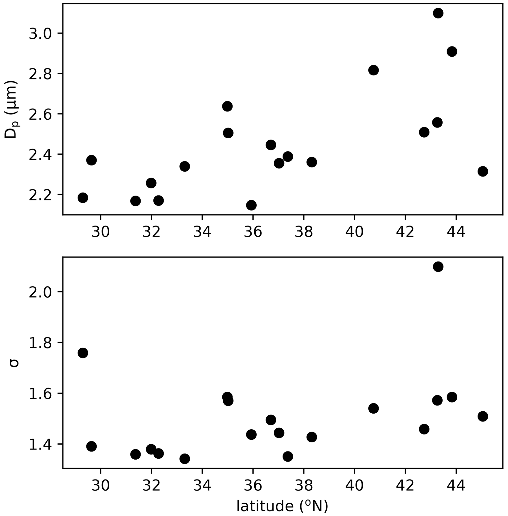
Figure 5Geometric mean diameter (Dp) and geometric standard deviation (σ) as a function of latitude for the number distribution of FBAP particles observed by WIBS over the continental USA in 2016.
3.3 Global emissions and burden
We implement both the population model and the statistical model in GEOS-Chem to calculate global emissions and burden of fungal spores and compare these results to those of the HS09 scheme. Table 3 shows an overview of all GEOS-Chem simulations, and Table 4 shows global spore emissions, burden and lifetime from the CTRL run for the three schemes as implemented in GEOS-Chem. Both the statistical model and the population model produce emissions that are about an order of magnitude lower (3.7 and 3.4 Tg yr−1, respectively) on the global scale than the HS09 scheme (31 Tg yr−1; note that we implement the scheme with the original coefficients in GEOS-Chem, and not the optimized version as in Sect. 2.4). These differences have several causes: first, there is a coarse mode in HS09, which contains 74 % of the emitted mass in that scheme (but note that the fine mode from HS09 alone contains about 2 times more emitted mass than the two new schemes). Then, there are different assumptions on the size distribution of spores, as discussed in Sect. 3.2. Finally, the locations of the observations differ: HS09 used observations from tropical forests, which are expected to show higher concentrations of spores than temperate ecosystems as used in the present study. The absence of observations from tropical ecosystems is a limitation on the new parameterizations, so more spore count data from those ecosystems would be very valuable for evaluating the new schemes and/or to develop emission parameterizations for tropical ecosystems.

Table 4Global emissions, burden and lifetime for fungal spores using the three different emission schemes. The different lifetimes for the HS09 scheme are for the coarse and fine modes, respectively.
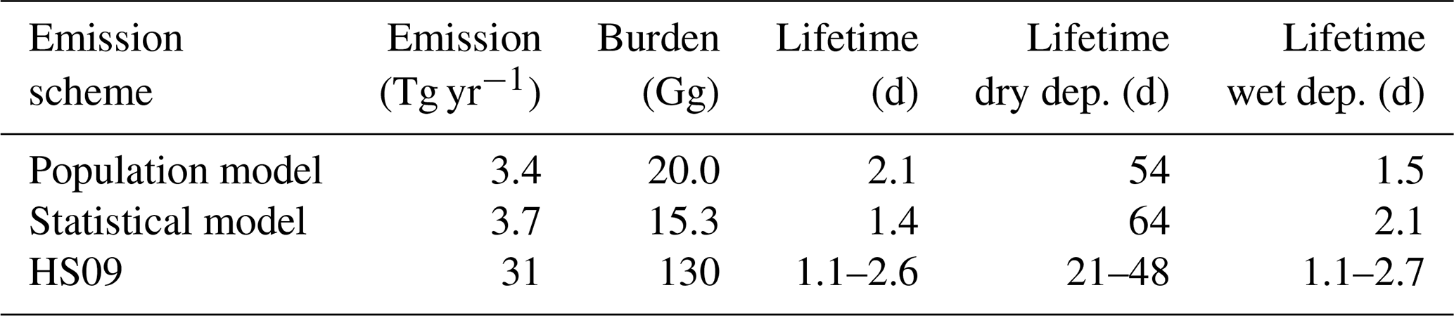
The HS09 scheme total spore emission of 31 Tg yr−1 (of which 8 Tg yr−1 are in the fine mode and 23 Tg yr−1 in the coarse mode, following sizes specified in that study) is 10 % higher in the current implementation than in the original study. This difference is due to different model meteorology (GEOS-4 versus MERRA2), LAI and year of simulation. Despite the slightly higher emissions in our simulations, we find that the burden is about 30 % lower than in the original study, due to more efficient wet deposition of coarse particles in the newer model version. Similar to the emissions, the burdens for the statistical and population model are also about an order of magnitude lower than the burden for the HS09 scheme. The fungal spore lifetime for the statistical model is lower than for the population model (1.4 vs. 2.1 d), because the statistical model emissions are more concentrated in regions that are characterized by high rainfall (i.e., the tropics), and therefore with faster wet removal of particles.
All three emission schemes yield a similar spatial pattern of annual mean emissions with emission peaks across the tropics and minor peaks in the southeastern USA, Europe and southeast Asia (Fig. 6). This similarity is not surprising, as all schemes use LAI as input, and in the tropics high temperatures accompany high specific humidity. The seasonal cycles in emissions and concentrations, however, show more pronounced differences between the schemes (Fig. 7). Over North America and Asia, for instance, emissions from the statistical and the HS09 model peak in July while those of the population model peak in August. These differences in emissions are reflected in the concentrations. Over North America, peak concentrations of spores from the statistical and the HS09 model peak 1 month after the emissions in August, but spores from the population model concentrations peak in September, with a secondary peak in November. These delays between emissions and concentrations are mainly caused by the occurrence of wet deposition (see Fig. S3); in months when high emissions coincide with high rainfall, the resulting concentrations may be lower than in months with somewhat lower emissions, but also with lower amounts of precipitation. Also, in Europe, the population model emissions start increasing later than in the other two schemes (May versus April), but when they increase it happens more rapidly. Over Asia, simulated concentrations from the statistical and the HS09 model follow quite different seasonal cycles than the population model, with the former two peaking in August and the latter in November. This is a consequence of the interplay between emissions and wet deposition: rainfall maxima occur in July and August in this region, related to the East Asian monsoon. Statistical model emissions show a peak during the same period, and therefore statistical model concentrations are still high. Population model emissions, on the other hand, are much weaker. The concentrations resulting from both models are similar, which is caused by the stronger wet deposition flux for the statistical model spores.

Figure 6Annual average fungal spore emissions and mass concentration from the statistical (a, b), the population (c, d) and the HS09 model (e, f).
Over South America, the statistical model predicts a stronger seasonal cycle in emissions than the population and the HS09 model, and also the timing differs, with the emissions from the statistical model showing a minimum in July and the other models in June. As a results of these different seasonal cycles in emissions, all models show different seasonal cycles in the concentrations. The statistical model shows peak concentrations from April through August, the population model peaks in July and August and the HS09 model in April. The statistical and population model yield minima during the transition period from the dry to the wet season and the wet season (October–February), while the HS09 model shows minimum concentrations in June. Since wet deposition in GEOS-Chem is size-dependent, it has a stronger influence on the spore concentrations from the HS09 scheme, due to the presence of a fine and a coarse mode (see Sect. 3.2). For the other two emission models, the modeled concentrations clearly result from the interplay between emissions and wet deposition during the seasons.
As a verification of our implementation of the statistical and population emission schemes, we compare the results of both schemes within the GEOS-Chem simulation to the AAAAI data from which they were developed. In addition, we also compare the results from the HS09 scheme as implemented in GEOS-Chem to the AAAAI data. Theoretically, one would expect near-perfect agreement here, but there are several factors, largely related to comparing a single observation with grid box average values, which can degrade this comparison. First, in GEOS-Chem, each 2∘ × 2.5∘ grid box can contain multiple land cover types, including land use types, like water surfaces, from which no spores are emitted. Including these land cover types would lead to an underestimate in grid box average spore emissions compared to emission at the AAAAI station in that grid box, which has been shown before to be an issue in the model–measurement comparison of deposition (Silva and Heald, 2018). To be able to make a fair comparison between grid boxes and point measurements, we run a simulation in which the grid boxes that partly contain water surfaces had a fully emitting land cover. Further, for the comparison of modeled and observed spore concentrations, several additional factors contribute to model vs. point measurement differences, including the exclusion of days with rain and wet deposition in the offline calculations, and in general differences in meteorology between the years of observations and simulation (2003–2008 vs. 2016).
We find that GEOS-Chem is able to reproduce the broad pattern in annual average fungal spore emissions over the USA, with high emissions in the east and low emissions in the west, for the emissions from both the statistical and the population model (Fig. 8). In the control simulation, both models show a negative bias compared to the emissions derived from the AAAAI observations (Fig. S4). The HS09 scheme also reproduces this pattern, but with a strong overestimation of number emissions over the whole USA (NMB = 10.1), even when looking at fine-mode spores only. This overestimate of number emissions is expected given the order of magnitude difference in emitted mass. We note that while the overestimate of emitted mass is largely driven by the inclusion of the coarse-mode emissions in HS09, which make up 75 % of the emissions based on the mannitol observations used to constrain that model, the overestimate in emitted spore numbers is mainly due to emissions in the fine mode. However, the observed size distribution data (see Sect. 3.2) seem inconsistent with this preponderance of fungal spores in the coarse mode; more work is needed to understand the size distribution of fungal spores and the efficiency with which spores are sampled by various measurement techniques. For the statistical and the population model, we find that the GEOS-Chem emissions have a small negative bias (NMB .01 and −0.08, respectively), but that the skill in reproducing seasonal variations at the AAAAI stations is low (r2=0.28 and 0.26, respectively). The latter can be explained by the fact that, although the combined seasonal cycle over all stations is reproduced well in the model fit (Fig. 4), the emission models do not capture the variations between stations that may result from, for instance, different land use (and vegetation) types surrounding the stations.
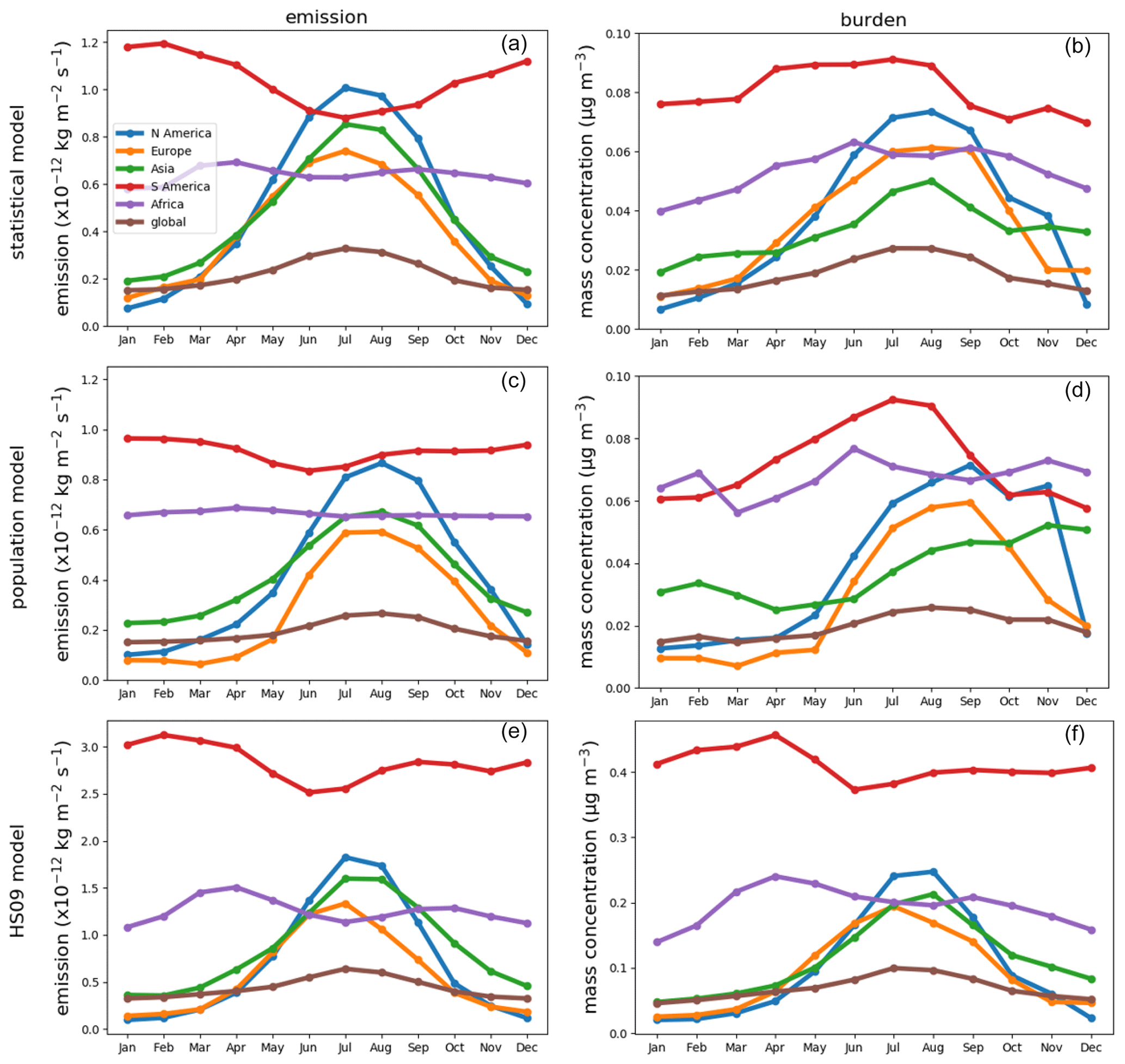
Figure 7Seasonal cycles of fungal spore emissions (a, c, e) and concentrations (b, d, f) for the statistical, the population and the HS09 model. Note the different scales on the y axis.
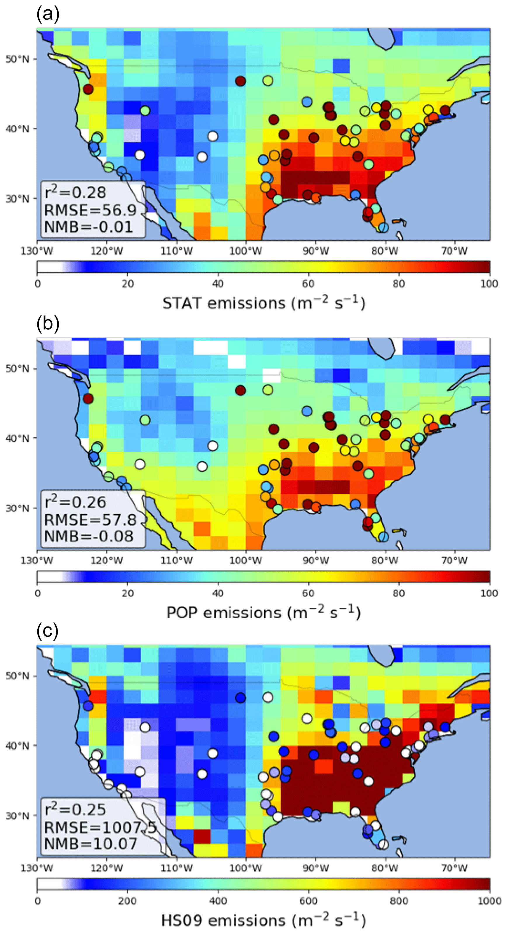
Figure 8Comparison of GEOS-Chem simulated emission fluxes of fungal spores to emission fluxes derived from AAAAI observations for the statistical model (a), the population model (b) and the HS09 model (c). Note the different scale for the bottom figure. Statistics describing the comparisons are shown inset.
We can conclude that the statistical model reproduces the magnitude and seasonal cycle of fungal spore emissions slightly better than the population model. We explore comparisons against independent measurements in Sect. 3.4 to identify whether one scheme has additional model skill over the other.
3.4 Validation with independent datasets: seasonal cycle and vertical profile
Since our models are based on observed spore counts from the United States, a validation with independent datasets is vital, particularly for other regions. Unfortunately, there are limited direct observations of fungal spore concentrations. Measurements of fluorescent biological aerosol particles (FBAPs) are available that can, in principle, be used for this purpose. However, caution is needed in the comparison with spore concentrations, because the fluorescence data cannot directly provide well-constrained spore counts (Huffman et al., 2020). Other biological particles (bacteria and pollen) as well as certain types of non-biological particles can contribute to these measurements as well, although with varying fluorescence efficiency and as a function of particle size and especially instrument operation and analysis procedures (Crawford et al., 2015; Perring et al., 2015; Savage et al., 2017; Toprak and Schnaiter, 2013). Further, weakly fluorescing spores can escape detection (Huffman et al., 2012). Therefore, we do not compare number concentrations directly but focus on seasonal cycles and vertical profiles instead, for which we show normalized time series and profiles. We applied min–max normalization, which scales all values to a range between 0 and 1.
Few observational studies exist that cover a full seasonal cycle or longer. Two of the available datasets were collected in Europe and thus provide particularly valuable validation of our models beyond the domain for which they have been developed. The first dataset used in this comparison is from a semi-rural site in Karlsruhe, Germany, where a WIBS-4 instrument was employed (Toprak and Schnaiter, 2013) from 1 April 2010 to 1 April 2011. In a boreal forest in Hyytiälä, Finland, a UV-APS was employed from 27 August 2009 to 17 April 2011 and the same instrument was used in a pine forest in Colorado, USA (Schumacher et al., 2013), from 20 July 2011 to 31 May 2012. Based on one distinct mode in their FBAP observations, Toprak and Schnaiter (2013) attributed their observations to a site-specific spore type. For the Hyytiälä site, Manninen et al. (2014) suggest that fungal spores strongly contribute to PBAP numbers, based on spore counts. No dominant contributor to the FBAP concentrations has been identified at the Colorado site. Our focus is on the normalized seasonal cycle, but we note that when comparing the absolute concentrations, we find a systematic low bias for the population and the statistical model and a high bias for the HS09 model. There are several reasons why a low bias in the model simulations is reasonable. First, as previously noted, the FBAP concentrations from the WIBS and UV-APS instruments do not only consist of spores but may contain bacteria and pollen (fragments) too, as well as interferences from non-biological particles. Second, at the Hyytiälä and Colorado sites, the instrument inlets were situated inside the canopy, where concentrations of bioaerosols are usually higher than above the canopy due to proximity to sources (Crawford et al., 2014; Gabey et al., 2010). GEOS-Chem, on the other hand, does not include a canopy model, so its results are representative of the lowest atmospheric layer above the canopy. Finally, as noted in Sect. 2.1, the spore count measurements at AAAAI sites, which are used here to constrain the emissions used in GEOS-Chem, are a lower limit given the size limits of the sampling. Unfortunately, there are no co-located fluorescence and spore count measurements that can be compared directly to explore these differences.
For the normalized seasonal cycle, we find similar results for all three sites (plotted as 20 d rolling means in Fig. 9). Table S2 shows that for the ground-based observations, the normalization factors are within a narrow range.
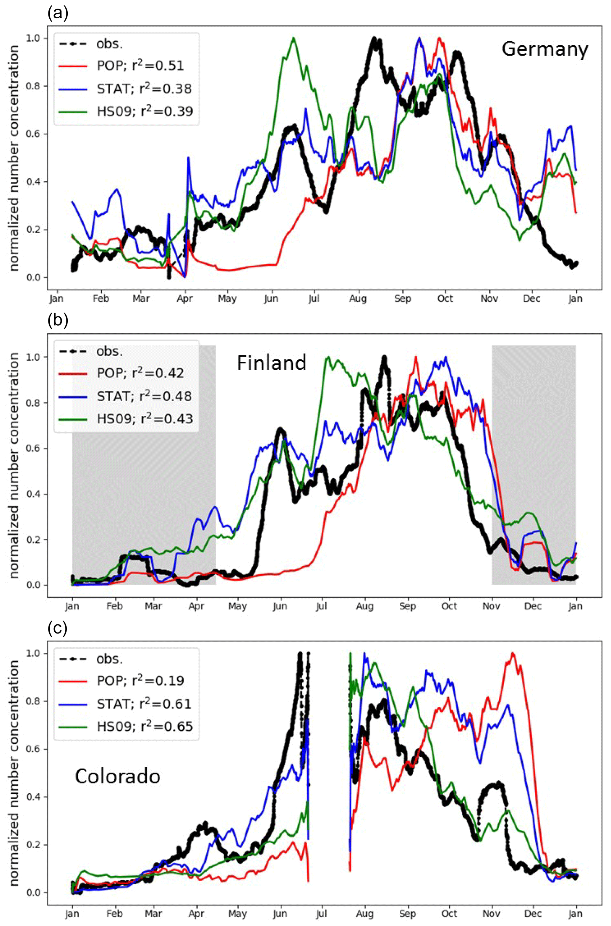
Figure 9Normalized seasonal cycle in fungal spore and FBAP concentrations in Germany, Finland and Colorado (see text for details). Observations (black) are compared to the simulated concentrations from the population model (red), the statistical model (blue) and the HS09 scheme (green). The shaded area indicates periods with snow cover; statistics are given for the snow-free period only.
Note that we correct for the fact that the emitting land fraction of the GEOS-Chem grid box over the Hyytiälä site is smaller than one, and that we exclude the period during which the ground surface was covered with snow at this site from the statistics, since this inhibits spore emission (Schumacher et al., 2013). For the Karlsruhe site, all model simulations capture the broad features of the seasonal cycles well, with low concentrations in winter (January to March), rising concentrations in spring, and peak concentrations in summer and fall (until October). The HS09 model, however, predicts peak concentrations in June, while the observations peak from August to October. The population model does not capture the rapid concentration increase in May and June. At Hyytiälä, the HS09 model shows a peak in July, which is not present in the observations or the other models, and the population model also misses the peak in early summer here. For both sites, all models show similar skill in capturing the seasonal variability. Only for the site in Germany does the population model capture the seasonal variability somewhat better than the other models.
At the site in Colorado, all models have difficulty capturing the average behavior shown in Fig. 9. The seasonal cycle at this site is composed of observations that span two calendar years, July 2011 to June 2012, which explains the sudden shift from high to low normalized concentrations in summer. For the period from January to July, all three models capture the concentration increase, with low concentrations from January to April, and an increase from May onwards. The statistical model reproduces the timing and relative magnitude of this growth particularly well. During the period from September through November, however, the statistical and population models fail to capture the relatively low spore concentrations. Only in December do all models capture the minimum in the concentrations that is present in the observations as well.
In addition, the agreement between the model and measurement strongly depends on the choice of the temperature threshold below which emissions are shut off for the statistical and the population model. In Sect. 3.1, we set this threshold to 0 ∘C, and here we evaluate the effect of setting no temperature threshold and a threshold of 5 ∘C, respectively. Figure S5 shows that setting no temperature threshold strongly degrades the model–measurement agreement, especially at the Karlsruhe site in December when modeled concentrations peak while FBAP concentrations actually have a minimum. For Hyytiälä, the model–measurement agreement decreases as well, but less than at the Karlsruhe site, because the period with snow cover was already excluded. On the other hand, when we set the threshold to 5 ∘C, both the statistical and the population model reproduce the seasonal cycles at both sites well, with r2 between 0.62 and 0.71. The fact that this relatively arbitrary choice makes such a big difference for the ability of the models to reproduce the observed seasonal cycle suggests that the low availability of AAAAI observations during winter severely limits the derivation of emission schemes from those data.
In conclusion, calculated spore concentrations from the population and the statistical model capture the seasonal variations in FBAP concentrations with skill comparable to the HS09 model, although assumptions on the temperature threshold below which no emissions occur have a large influence on the performance of the former two models.
Vertical profiles of FBAP are available for several campaigns over the continental United States, including SEAC4RS (August–September 2013; Ziemba et al., 2016) and IDEAS (September–October 2013; Twohy et al., 2016), and over the North Atlantic from the NAAMES 2015, 2016 and 2017 campaigns (Behrenfeld et al., 2019). The SEAC4RS and IDEAS campaigns enable us to evaluate how well the model captures the vertical transport of fungal spore-like fluorescent particles close to the source and the NAAMES campaigns characterize the transport of spores through continental outflow toward the North Atlantic. The North Atlantic Aerosol and Marine Ecosystems Study (NAAMES) included aerosol measurements from the NASA Wallops Flight Facility (WFF) C-130 based in St. John's, Newfoundland, Canada. Flight campaigns occurred in the fall of 2015 (9 through 23 November), late spring of 2016 (18 May through 1 June), and late summer of 2017 (28 August through 19 September). The WIBS sampled iso-kinetically through a shrouded solid-diffuser inlet that efficiently samples particles with up to 5 µm aerodynamic diameter (McNaughton et al., 2007). WIBS was operated at a constant sample flow rate, and concentrations were corrected to standard temperature and pressure (Ziemba et al., 2016). To exclude the possible influence of biomass burning, which can produce fluorescent aerosols (Savage et al., 2017), only the observations for which simultaneous acetonitrile concentrations are below 200 ppt were used. Cloud-contaminated samples have been removed using coincident measurements from a set of wing-mounted optical probes.
Because of the same issues with the interpretation of FBAP measurements as mentioned above, we compare mean observed and simulated normalized vertical profiles for each campaign. For the flight campaigns, all normalization factors are within a factor of 3 from each other, with the exception of SEAC4RS, for which the factor is an order of magnitude lower (Table S2). When we compare the simulated concentrations with the observed profiles, we see that simulated normalized concentrations from GEOS-Chem generally agree well with the observed concentrations from the SEAC4RS and IDEAS flights (Fig. 10). For the SEAC4RS flights, all models capture the observed vertical profile. Potential temperature profiles agree well between model and observations, which gives confidence in the correct representation of convective transport by the model. For the IDEAS flights, the model slightly overestimates normalized concentrations around 650 hPa and underestimates them between 600 and 500 hPa, but these differences fall within the variability in the observations. Overall, the model appears to generally capture the vertical transport of spores over their source regions. The dilution factor between BL and FT from these modeled profiles is about 0.3 for the SEAC4RS and about 0.6 for the IDEAS campaign (in Sect. 4 we explore how the use of these dilution factors would impact our emissions derivation).
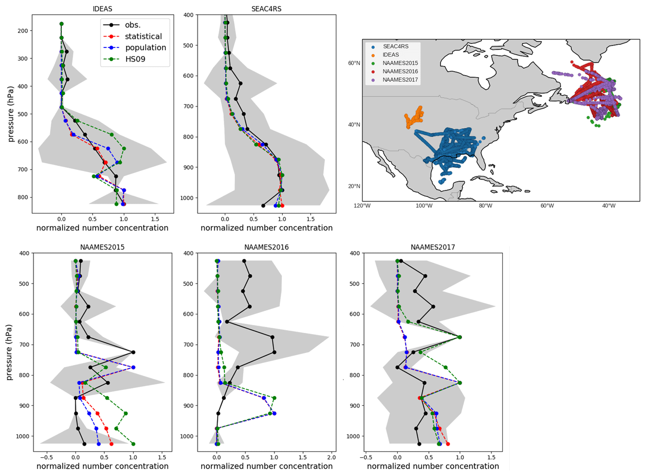
Figure 10Normalized vertical profiles of fluorescent biological aerosol particles (FBAPs) from five campaigns (black) compared with normalized vertical profiles of fungal spore number concentrations from three model simulations: the population model (blue), the statistical model (red) and the HS09 model (green). Normalized profiles are obtained by applying min–max normalization, which scales all values to a range between 0 and 1. Standard deviation of observations in each 50 hPa pressure bin are shown in grey. The upper-right panel shows the flight tracks for each campaign.
For the campaigns over the North Atlantic, the model simulations underestimate the absolute concentrations (which are small; <10 L−1) for all years and emissions schemes, with the exception of the HS09 scheme for the 2017 campaign. All years show concentration maxima between the 800 and 600 hPa levels (Fig. 10), which are the result of continental outflow of fluorescent particles. The simulations generally do not capture these relative profiles and show decreasing concentrations with height, with the exception of 2015, when all simulations reproduce the lower-tropospheric peak between 650 and 850 hPa, and 2017, when model simulations for the HS09 scheme peak at that same level. Given that the model captures the potential temperature profile for the 2016 campaign, it seems unlikely that local convective transport is the reason for the mismatch. Rather, it suggests that long-range transport of fungal spores and processing through continental outflow may not be well represented by the model. This points to the need for further investigation of the transport and solubility of fungal spores.
We have developed new emission schemes for fungal spores for inclusion in regional and global models, based on a previously unexplored dataset of fungal spore counts at 66 locations across the United States. First, we calculated fungal spore emissions from observed concentrations by applying the boundary layer equilibrium assumption, yielding annual average fungal spore emissions over all stations of 62 ± 31 m−2 s−1. Then, we developed two schemes to simulate the emissions of fungal spores at seasonal timescales over a wide range of land use types: a population model that simulates the growth of fungi and the production of spores and their emissions as a function of temperature, LAI and friction velocity, and a statistical model that relates spore emissions to meteorological and land surface drivers. The population model shows better skill at reproducing the seasonal cycle in the emissions than the statistical model, whereas both outperform the HS09 scheme.
After implementation in GEOS-Chem, we used the new schemes to calculate global emissions and burden of fungal spores. The results suggest that fungal spores contribute less to the organic aerosol budget of the atmosphere and are likely less important for cloud and precipitation formation than previously estimated in models. For the population and the statistical model, we estimate emissions of 3.4 and 3.7 Tg yr−1, respectively, both of which are substantially lower than the estimate of 31 Tg yr−1, generated by the HS09 scheme. These differences are largely the result of different assumptions about size, and the use of different observational constraints (fungal spore counts in this work, versus mannitol concentrations in HS09). Additionally, the data on which the HS09 scheme were developed contained a large number of data points from tropical forests, which are absent in the AAAAI dataset. This means that the simulated emissions over tropical forests from the statistical and population model are in fact extrapolations based on data from temperate ecosystems.
However, these numbers are sensitive to our assumptions on (1) the derivation of fluxes from concentrations, (2) emission model formulation, and (3) transport and removal processes in the GEOS-Chem chemical transport model. Regarding the former, we assumed a dilution factor of 0.1 between the BL and FT that was derived from a few observations only. Lower assumed values do not have a significant impact on the calculated fluxes, as such a low dilution already yields upper limit estimates for the calculated emissions. We can also estimate the dilution factor inherent to our GEOS-Chem simulations, by comparing BL and FT fungal spore concentrations over land, and find that this value is typically ∼ 0.3. Using this value in our derivation of emissions would decrease the average calculated flux to 49 ± 25 m−2 s−1, which translates to 21 % lower global emissions for both the population and statistical model (Table S1). This analysis shows that uncertainties in the dilution factor directly impact the modeled emission fluxes but do not change our finding that these fluxes are an order of magnitude or more lower than those estimated in previous studies. Large uncertainties also remain in the efficiency of wet removal, since both the representation of precipitation and the formulation of wet deposition schemes are complex issues for global models. Moreover, knowledge on aging of fungal spores, and the consequences for their behavior in the atmosphere, is limited. Exposure to high relative humidity for several hours may lead to the rupturing of spores, and the formation of cloud-active sub-spore particles (China et al., 2016; Lawler et al., 2020). Further, photo-oxidants, UV-radiation and temperature changes may also induce physical and chemical transformations in bioaerosols (Fröhlich-Nowoisky et al., 2016), potentially altering their solubility. We test the sensitivity of the modeled fungal spore burden to wet deposition by changing the rain-out efficiency from 1 to 0. This change from full to no solubility has a large effect on the global burden (leading to an increase of 28 % and 31 % for the population and the statistical model, respectively, when spores are assumed non-soluble; Table S1), but it has little effect on the normalized vertical profiles. This suggests that current observations are insufficient to constrain the solubility of spores in the model.
Limited validation of our model results is possible with datasets outside the US domain. For two European sites, we find that the population model and the statistical model reproduce the seasonal cycle in FBAP concentrations with comparable skill to the HS09 model, although poor constraints on emissions in winter prohibit more definitive conclusions. A comparison with vertical FBAP profiles shows that normalized concentration profiles are represented well over source areas, but that the continental outflow of FBAP over the North Atlantic is not captured well by our model, suggesting a need to further investigate the transport and removal of fungal spores. Uncertainties in the spore count data which form the basis for the emission schemes and in the attribution of fluorescent measurements to spore concentrations prohibit a more quantitative evaluation of the modeled spore concentrations.
Although our new emission schemes are based on the largest available database of spore counts, there remain considerable uncertainties in our characterization of the fungal spore bioaerosol budget. Additional efforts are needed to improve our understanding of the impacts of fungal spores on atmospheric processes. First, more flux measurements of fungal spores over forests and other ecosystems would be very valuable to quantitatively evaluate the magnitude of the flux of spores into the atmosphere. Further, there is a critical need for long-term concentration measurements for locations that are not included in the AAAAI dataset, particularly in areas with high simulated fluxes, such as southeast Asia, and in ecosystems such as tropical forests, for which very little data are currently available. Further improvements in FBAP measurements to be able to more confidently extract fungal spore concentrations for further comparison would be useful. Finally, our analysis points out that there remain critical gaps in our understanding of long-range transport of spores, which calls for further research efforts in convective transport, cloud processing and wet removal of fungal spores.
The GEOS-Chem model code is available at http://acmg.seas.harvard.edu/geos/ (last access: 7 June 2020). The spore count data are available from the AAAAI upon request. FBAP data are available from the references as cited in the text.
The supplement related to this article is available online at: https://doi.org/10.5194/acp-21-4381-2021-supplement.
RHHJ and CLH designed the study. RHHJ performed the data analysis and the model simulations. ALS, AEP, JAH, ESR, CHT and LDZ provided spore count data and FBAP measurements used in the analysis. RHHJ and CLH wrote the paper with input from the co-authors.
The authors declare that they have no conflict of interest.
We thank Will Porter for discussion of the regression analysis, and Martin Schnaiter and Emre Toprak for sharing the Karlsruhe WIBS data. We gratefully acknowledge the use of the American Academy of Allergy, Asthma and Immunology (AAAAI) spore count data. Colorado and Finland data were collected with support from the MPIC and the Mainz Bioaerosol Laboratory (MBAL), with special thanks to Ulrich Pöschl and Christopher Pöhlker.
This research has been supported by the National Science Foundation (grant no. AGS-1564495). Anne E. Perring was supported by the NOAA Atmospheric Composition and Climate Program and the NOAA Health of the Atmosphere Program. J. Alex Huffman was supported by institutional funding from the University of Denver and the Max Planck Institute for Chemistry (MPIC). SEAC4RS measurements were supported by NASA's Upper Atmosphere Research Program, Radiation Sciences Program, and Tropospheric Chemistry Program. NAAMES measurements were supported by the NASA Earth Venture Suborbital Program.
This paper was edited by Corinna Hoose and reviewed by three anonymous referees.
Ahlm, L., Krejci, R., Nilsson, E. D., Mårtensson, E. M., Vogt, M., and Artaxo, P.: Emission and dry deposition of accumulation mode particles in the Amazon Basin, Atmos. Chem. Phys., 10, 10237–10253, https://doi.org/10.5194/acp-10-10237-2010, 2010.
Bakwin, P. S., Davis, K. J., Yi, C., Wofsy, S. C., Munger, J. W., Haszpra, L., and Barcza, Z.: Regional carbon dioxide fluxes from mixing ratio data, Tellus B, 56, 301–311, https://doi.org/10.1111/j.1600-0889.2004.00111.x, 2004.
Behrenfeld, M. J., Moore, R. H., Hostetler, C. A., Graff, J., Gaube, P., Russell, L. M., Chen, G., Doney, S. C., Giovannoni, S., Liu, H., Proctor, C., Bolaños, L. M., Baetge, N., Davie-Martin, C., Westberry, T. K., Bates, T. S., Bell, T. G., Bidle, K. D., Boss, E. S., Brooks, S. D., Cairns, B., Carlson, C., Halsey, K., Harvey, E. L., Hu, C., Karp-Boss, L., Kleb, M., Menden-Deuer, S., Morison, F., Quinn, P. K., Scarino, A. J., Anderson, B., Chowdhary, J., Crosbie, E., Ferrare, R., Hair, J. W., Hu, Y., Janz, S., Redemann, J., Saltzman, E., Shook, M., Siegel, D. A., Wisthaler, A., Martin, M. Y., and Ziemba, L.: The North Atlantic Aerosol and Marine Ecosystem Study (NAAMES): Science Motive and Mission Overview, Front. Mar. Sci., 6, 122, https://doi.org/10.3389/fmars.2019.00122, 2019.
Betts, A. K.: Idealized Model for Equilibrium Boundary Layer over Land, J. Hydrometeorol., 1, 507–523, https://doi.org/10.1175/1525-7541(2000)001<0507:IMFEBL>2.0.CO;2, 2000.
Boddy, L., Büntgen, U., Egli, S., Gange, A. C., Heegaard, E., Kirk, P. M., Mohammad, A., and Kauserud, H.: Climate variation effects on fungal fruiting, Fungal Ecol., 10, 20–33, https://doi.org/10.1016/j.funeco.2013.10.006, 2014.
Burrows, S. M., Butler, T., Jöckel, P., Tost, H., Kerkweg, A., Pöschl, U., and Lawrence, M. G.: Bacteria in the global atmosphere – Part 2: Modeling of emissions and transport between different ecosystems, Atmos. Chem. Phys., 9, 9281–9297, https://doi.org/10.5194/acp-9-9281-2009, 2009.
Carotenuto, F., Georgiadis, T., Gioli, B., Leyronas, C., Morris, C. E., Nardino, M., Wohlfahrt, G., and Miglietta, F.: Measurements and modeling of surface–atmosphere exchange of microorganisms in Mediterranean grassland, Atmos. Chem. Phys., 17, 14919–14936, https://doi.org/10.5194/acp-17-14919-2017, 2017.
China, S., Wang, B., Weis, J., Rizzo, L., Brito, J., Cirino, G. G., Kovarik, L., Artaxo, P., Gilles, M. K., and Laskin, A.: Rupturing of biological spores as a source of secondary particles in Amazonia, Environ. Sci. Technol., 50, 12179–12186, https://doi.org/10.1021/acs.est.6b02896, 2016.
China, S., Burrows, S. M., Wang, B., Harder, T. H., Weis, J., Tanarhte, M., Rizzo, L. V., Brito, J., Cirino, G. G., Ma, P.-L., Cliff, J., Artaxo, P., Gilles, M. K., and Laskin, A.: Fungal spores as a source of sodium salt particles in the Amazon basin, Nat. Commun., 9, 4793, https://doi.org/10.1038/s41467-018-07066-4, 2018.
Crawford, I., Robinson, N. H., Flynn, M. J., Foot, V. E., Gallagher, M. W., Huffman, J. A., Stanley, W. R., and Kaye, P. H.: Characterisation of bioaerosol emissions from a Colorado pine forest: results from the BEACHON-RoMBAS experiment, Atmos. Chem. Phys., 14, 8559–8578, https://doi.org/10.5194/acp-14-8559-2014, 2014.
Crawford, I., Ruske, S., Topping, D. O., and Gallagher, M. W.: Evaluation of hierarchical agglomerative cluster analysis methods for discrimination of primary biological aerosol, Atmos. Meas. Tech., 8, 4979–4991, https://doi.org/10.5194/amt-8-4979-2015, 2015.
Damialis, A., Mohammad, A. B., Halley, J. M., and Gange, A. C.: Fungi in a changing world: growth rates will be elevated, but spore production may decrease in future climates, Int. J. Biometeorol., 59, 1157–1167, https://doi.org/10.1007/s00484-014-0927-0, 2015.
DeLeon-Rodriguez, N., Lathem, T. L., Rodriguez, L. M., Barazesh, J. M., Anderson, B. E., Beyersdorf, A. J., Ziemba, L. D., Bergin, M., Nenes, A., and Konstantinidis, K. T.: Microbiome of the upper troposphere: Species composition and prevalence, effects of tropical storms, and atmospheric implications, P. Natl. Acad. Sci. USA, 110, 2575–2580, https://doi.org/10.1073/pnas.1212089110, 2013.
Després, V., Huffman, J., Burrows, S., Hoose, C., Safatov, A., Buryak, G., Fröhlich-Nowoisky, J., Elbert, W., Andreae, M., Pöschl, U., and Ruprecht, J.: Primary biological aerosol particles in the atmosphere: a review, Tellus B, 64, 15598 https://doi.org/10.3402/tellusb.v64i0.15598, 2012.
Elbert, W., Taylor, P. E., Andreae, M. O., and Pöschl, U.: Contribution of fungi to primary biogenic aerosols in the atmosphere: wet and dry discharged spores, carbohydrates, and inorganic ions, Atmos. Chem. Phys., 7, 4569–4588, https://doi.org/10.5194/acp-7-4569-2007, 2007.
Fisher, M. C., Henk, D. A., Briggs, C. J., Brownstein, J. S., Madoff, L. C., McCraw, S. L., and Gurr, S. J.: Emerging fungal threats to animal, plant and ecosystem health, Nature, 484, 186–194, https://doi.org/10.1038/nature10947, 2012.
Fröhlich-Nowoisky, J., Kampf, C. J., Weber, B., Huffman, J. A., Pöhlker, C., Andreae, M. O., Lang-Yona, N., Burrows, S. M., Gunthe, S. S., Elbert, W., Su, H., Hoor, P., Thines, E., Hoffmann, T., Desprès, V. R., and Pöschl, U.: Bioaerosols in the Earth system: Climate, health, and ecosystem interactions, Atmos. Res., 182, 346–376, https://doi.org/10.1016/j.atmosres.2016.07.018, 2016.
Gabey, A. M., Gallagher, M. W., Whitehead, J., Dorsey, J. R., Kaye, P. H., and Stanley, W. R.: Measurements and comparison of primary biological aerosol above and below a tropical forest canopy using a dual channel fluorescence spectrometer, Atmos. Chem. Phys., 10, 4453–4466, https://doi.org/10.5194/acp-10-4453-2010, 2010.
Gange, A. C., Gange, E. G., Sparks, T. H., and Boddy, L.: Rapid and Recent Changes in Fungal Fruiting Patterns, Science, 316, p. 71, https://doi.org/10.1126/science.1137489, 2007.
Geagea, L., Huber, L., Sache, I., Flura, D., McCartney, H. A., and Fitt, B. D. L.: Influence of simulated rain on dispersal of rust spores from infected wheat seedlings, Agr. Forest Meteorol., 101, 53–66, https://doi.org/10.1016/S0168-1923(99)00155-0, 2000.
Gelaro, R., McCarty, W., Suárez, M. J., Todling, R., Molod, A., Takacs, L., Randles, C. A., Darmenov, A., Bosilovich, M. G., Reichle, R., Wargan, K., Coy, L., Cullather, R., Draper, C., Akella, S., Buchard, V., Conaty, A., da Silva, A. M., Gu, W., Kim, G.-K., Koster, R., Lucchesi, R., Merkova, D., Nielsen, J. E., Partyka, G., Pawson, S., Putman, W., Rienecker, M., Schubert, S. D., Sienkiewicz, M., and Zhao, B.: The Modern-Era Retrospective Analysis for Research and Applications, Version 2 (MERRA-2), J. Climate, 30, 5419–5454, https://doi.org/10.1175/JCLI-D-16-0758.1, 2017.
Haga, D. I., Burrows, S. M., Iannone, R., Wheeler, M. J., Mason, R. H., Chen, J., Polishchuk, E. A., Pöschl, U., and Bertram, A. K.: Ice nucleation by fungal spores from the classes Agaricomycetes, Ustilaginomycetes, and Eurotiomycetes, and the effect on the atmospheric transport of these spores, Atmos. Chem. Phys., 14, 8611–8630, https://doi.org/10.5194/acp-14-8611-2014, 2014.
Heald, C. L. and Spracklen, D. V.: Atmospheric budget of primary biological aerosol particles from fungal spores, Geophys. Res. Lett., 36, L09806, https://doi.org/10.1029/2009GL037493, 2009.
Helliker, B. R., Berry, J. A., Betts, A. K., Bakwin, P. A., Davis, K., Denning, A. S., Ehleringer, J. R., Miller, J. B., Butler, M. B., and Ricciuto, D. M.: Estimates of net CO2 flux by application of equilibrium boundary layer concepts to CO2 and water vapor measurements from a tall tower, J. Geophys. Res., 109, D20106, https://doi.org/10.1029/2004JD004532, 2004.
Hirst, J. M.: An Automatic Volumetric Spore Trap, Ann. Appl. Biol., 39, 257–265, https://doi.org/10.1111/j.1744-7348.1952.tb00904.x, 1952.
Hoose, C., Kristjánsson, J. E., and Burrows, S. M.: How important is biological ice nucleation in clouds on a global scale?, Environ. Res. Lett., 5, 024009, https://doi.org/10.1088/1748-9326/5/2/024009, 2010.
Huffman, J. A., Sinha, B., Garland, R. M., Snee-Pollmann, A., Gunthe, S. S., Artaxo, P., Martin, S. T., Andreae, M. O., and Pöschl, U.: Size distributions and temporal variations of biological aerosol particles in the Amazon rainforest characterized by microscopy and real-time UV-APS fluorescence techniques during AMAZE-08, Atmos. Chem. Phys., 12, 11997–12019, https://doi.org/10.5194/acp-12-11997-2012, 2012.
Huffman, J. A., Prenni, A. J., DeMott, P. J., Pöhlker, C., Mason, R. H., Robinson, N. H., Fröhlich-Nowoisky, J., Tobo, Y., Després, V. R., Garcia, E., Gochis, D. J., Harris, E., Müller-Germann, I., Ruzene, C., Schmer, B., Sinha, B., Day, D. A., Andreae, M. O., Jimenez, J. L., Gallagher, M., Kreidenweis, S. M., Bertram, A. K., and Pöschl, U.: High concentrations of biological aerosol particles and ice nuclei during and after rain, Atmos. Chem. Phys., 13, 6151–6164, https://doi.org/10.5194/acp-13-6151-2013, 2013.
Huffman, J. A., Perring, A. E., Savage, N. J., Clot, B., Crouzy, B., Tummon, F., Shoshanim, O., Damit, B., Schneider, J., Sivaprakasam, V., Zawadowicz, M. A., Crawford, I., Gallagher, M., Topping, D., Doughty, D. C., Hill, S. C., and Pan, Y.: Real-time sensing of bioaerosols: Review and current perspectives, Aerosol Sci. Technol., 54, 465–495, https://doi.org/10.1080/02786826.2019.1664724, 2020.
Hummel, M., Hoose, C., Gallagher, M., Healy, D. A., Huffman, J. A., O'Connor, D., Pöschl, U., Pöhlker, C., Robinson, N. H., Schnaiter, M., Sodeau, J. R., Stengel, M., Toprak, E., and Vogel, H.: Regional-scale simulations of fungal spore aerosols using an emission parameterization adapted to local measurements of fluorescent biological aerosol particles, Atmos. Chem. Phys., 15, 6127–6146, https://doi.org/10.5194/acp-15-6127-2015, 2015.
Jacobson, M. Z. and Streets, D. G.: Influence of future anthropogenic emissions on climate, natural emissions, and air quality, J. Geophys. Res.-Atmos., 114, D08118, https://doi.org/10.1029/2008JD011476, 2009.
Jaenicke, R.: Abundance of Cellular Material and Proteins in the Atmosphere, Science, 308, 73–73, https://doi.org/10.1126/science.1106335, 2005.
Jones, A. M. and Harrison, R. M.: The effects of meteorological factors on atmospheric bioaerosol concentrations – a review, Sci. Total Environ., 326, 151–180, https://doi.org/10.1016/j.scitotenv.2003.11.021, 2004.
Kauserud, H., Stige, L. C., Vik, J. O., Økland, R. H., Høiland, K., and Stenseth, N. Chr.: Mushroom fruiting and climate change, P. Natl. Acad. Sci. USA, 105, 3811–3814, https://doi.org/10.1073/pnas.0709037105, 2008.
Keller, C. A., Long, M. S., Yantosca, R. M., Da Silva, A. M., Pawson, S., and Jacob, D. J.: HEMCO v1.0: a versatile, ESMF-compliant component for calculating emissions in atmospheric models, Geosci. Model Dev., 7, 1409–1417, https://doi.org/10.5194/gmd-7-1409-2014, 2014.
Lawler, M. J., Draper, D. C., and Smith, J. N.: Atmospheric fungal nanoparticle bursts, Sci. Adv., 6, eaax9051, https://doi.org/10.1126/sciadv.aax9051, 2020.
Levetin, E.: Methods for aeroallergen sampling, Curr. Allergy Asthma R., 4, 376–383, https://doi.org/10.1007/s11882-004-0088-z, 2004.
Liu, H., Jacob, D. J., Bey, I., and Yantosca, R. M.: Constraints from 210Pb and 7Be on wet deposition and transport in a global three-dimensional chemical tracer model driven by assimilated meteorological fields, J. Geophys. Res.-Atmos., 106, 12109–12128, https://doi.org/10.1029/2000JD900839, 2001.
Löbs, N., Barbosa, C. G. G., Brill, S., Walter, D., Ditas, F., de Oliveira Sá, M., de Araújo, A. C., de Oliveira, L. R., Godoi, R. H. M., Wolff, S., Piepenbring, M., Kesselmeier, J., Artaxo, P., Andreae, M. O., Pöschl, U., Pöhlker, C., and Weber, B.: Aerosol measurement methods to quantify spore emissions from fungi and cryptogamic covers in the Amazon, Atmos. Meas. Tech., 13, 153–164, https://doi.org/10.5194/amt-13-153-2020, 2020.
Manninen, H. E., Sihto-Nissilä, S.-L., Hiltunen, V., Aalto, P. P., Kulmala, M., Petäjä, T., Manninen, H. E., Bäck, J., Hari, P., Huffman, J. A., Huffman, J. A., Saarto, A., Pessi, A.-M., and Hidalgo, P. J.: Patterns in airborne pollen and other primary biological aerosol particles (PBAP), and their contribution to aerosol mass and number in a boreal forest, Boreal Environ. Res., 19, 383–405, 2014.
McNaughton, C. S., Clarke, A. D., Howell, S. G., Pinkerton, M., Anderson, B., Thornhill, L., Hudgins, C., Winstead, E., Dibb, J. E., Scheuer, E., and Maring, H.: Results from the DC-8 Inlet Characterization Experiment (DICE): Airborne Versus Surface Sampling of Mineral Dust and Sea Salt Aerosols, Aerosol Sci. Technol., 41, 136–159, https://doi.org/10.1080/02786820601118406, 2007.
Mesinger, F., DiMego, G., Kalnay, E., Mitchell, K., Shafran, P. C., Ebisuzaki, W., Jović, D., Woollen, J., Rogers, E., Berbery, E. H., Ek, M. B., Fan, Y., Grumbine, R., Higgins, W., Li, H., Lin, Y., Manikin, G., Parrish, D., and Shi, W.: North American Regional Reanalysis, B. Am. Meteorol. Soc., 87, 343–360, https://doi.org/10.1175/BAMS-87-3-343, 2006.
Morris, C. E., Conen, F., Alex Huffman, J., Phillips, V., Pöschl, U., and Sands, D. C.: Bioprecipitation: a feedback cycle linking Earth history, ecosystem dynamics and land use through biological ice nucleators in the atmosphere, Glob. Change Biol., 20, 341–351, https://doi.org/10.1111/gcb.12447, 2014.
Myneni, R. B., Knyazikhin, Y., and Park, T.: MCD15A3H MODIS/Terra+Aqua Leaf Area Index/FPAR 4-day L4 Global 500m SIN Grid V006, distributed by NASA EOSDIS Land Processes DAAC, https://doi.org/10.5067/MODIS/MCD15A3H.006, 2015.
Myriokefalitakis, S., Fanourgakis, G., and Kanakidou, M.: The Contribution of Bioaerosols to the Organic Carbon Budget of the Atmosphere, in: Perspectives on Atmospheric Sciences, edited by: Karacostas, T., Bais, A., and Nastos, P. T., Springer International Publishing, Cham, Germany, 845–851, https://doi.org/10.1007/978-3-319-35095-0_121, 2017.
Newville, M., Stensitzki, T., Allen, D. B., and Ingargiola, A.: LMFIT: Non-Linear Least-Square Minimization and Curve-Fitting for Python, Zenodo, https://doi.org/10.5281/zenodo.11813, 2014.
Olson, D. M., Dinerstein, E., Wikramanayake, E. D., Burgess, N. D., Powell, G. V. N., Underwood, E. C., D'amico, J. A., Itoua, I., Strand, H. E., Morrison, J. C., Loucks, C. J., Allnutt, T. F., Ricketts, T. H., Kura, Y., Lamoreux, J. F., Wettengel, W. W., Hedao, P., and Kassem, K. R.: Terrestrial Ecoregions of the World: A New Map of Life on Earth: A new global map of terrestrial ecoregions provides an innovative tool for conserving biodiversity, BioScience, 51, 933–938, https://doi.org/10.1641/0006-3568(2001)051[0933:TEOTWA]2.0.CO;2, 2001.
O'Sullivan, D., Murray, B. J., Ross, J. F., Whale, T. F., Price, H. C., Atkinson, J. D., Umo, N. S., and Webb, M. E.: The relevance of nanoscale biological fragments for ice nucleation in clouds, Sci. Rep., 5, 8082, https://doi.org/10.1038/srep08082, 2015.
Perring, A. E., Schwarz, J. P., Baumgardner, D., Hernandez, M. T., Spracklen, D. V., Heald, C. L., Gao, R. S., Kok, G., McMeeking, G. R., McQuaid, J. B., and Fahey, D. W.: Airborne observations of regional variation in fluorescent aerosol across the United States, J. Geophys. Res.-Atmos., 120, 1153–1170, https://doi.org/10.1002/2014JD022495, 2015.
Porter, W. C., Heald, C. L., Cooley, D., and Russell, B.: Investigating the observed sensitivities of air-quality extremes to meteorological drivers via quantile regression, Atmos. Chem. Phys., 15, 10349–10366, https://doi.org/10.5194/acp-15-10349-2015, 2015.
Pöschl, U., Martin, S. T., Sinha, B., Chen, Q., Gunthe, S. S., Huffman, J. A., Borrmann, S., Farmer, D. K., Garland, R. M., Helas, G., Jimenez, J. L., King, S. M., Manzi, A., Mikhailov, E., Pauliquevis, T., Petters, M. D., Prenni, A. J., Roldin, P., Rose, D., Schneider, J., Su, H., Zorn, S. R., Artaxo, P., and Andreae, M. O.: Rainforest aerosols as biogenic nuclei of clouds and precipitation in the Amazon, Science, 329, 1513–1516, https://doi.org/10.1126/science.1191056, 2010.
Pratt, K. A., DeMott, P. J., French, J. R., Wang, Z., Westphal, D. L., Heymsfield, A. J., Twohy, C. H., Prenni, A. J., and Prather, K. A.: In situ detection of biological particles in cloud ice-crystals, Nat. Geosci., 2, 398–401, https://doi.org/10.1038/ngeo521, 2009.
Prenni, A. J., Petters, M. D., Kreidenweis, S. M., Heald, C. L., Martin, S. T., Artaxo, P., Garland, R. M., Wollny, A. G., and Poschl, U.: Relative roles of biogenic emissions and Saharan dust as ice nuclei in the Amazon basin, Nat. Geosci., 2, 402–405, https://doi.org/10.1038/ngeo517, 2009.
Prenni, A. J., Tobo, Y., Garcia, E., DeMott, P. J., Huffman, J. A., McCluskey, C. S., Kreidenweis, S. M., Prenni, J. E., Pöhlker, C., and Pöschl, U.: The impact of rain on ice nuclei populations at a forested site in Colorado, Geophys. Res. Lett., 40, 227–231, https://doi.org/10.1029/2012GL053953, 2013.
Pringle, A., Patek, S. N., Fischer, M., Stolze, J., and Money, N. P.: The captured launch of a ballistospore, Mycologia, 97, 866–871, https://doi.org/10.1080/15572536.2006.11832777, 2005.
Reinmuth-Selzle, K., Kampf, C. J., Lucas, K., Lang-Yona, N., Fröhlich-Nowoisky, J., Shiraiwa, M., Lakey, P. S. J., Lai, S., Liu, F., Kunert, A. T., Ziegler, K., Shen, F., Sgarbanti, R., Weber, B., Bellinghausen, I., Saloga, J., Weller, M. G., Duschl, A., Schuppan, D., and Pöschl, U.: Air Pollution and Climate Change Effects on Allergies in the Anthropocene: Abundance, Interaction, and Modification of Allergens and Adjuvants, Environ. Sci. Technol., 51, 4119–4141, https://doi.org/10.1021/acs.est.6b04908, 2017.
Samake, A., Uzu, G., Martins, J. M. F., Calas, A., Vince, E., Parat, S., and Jaffrezo, J. L.: The unexpected role of bioaerosols in the Oxidative Potential of PM, Sci. Rep., 7, 10978, https://doi.org/10.1038/s41598-017-11178-0, 2017.
Sarda-Estève, R., Baisnée, D., Guinot, B., Sodeau, J., O'Connor, D., Belmonte, J., Besancenot, J.-P., Petit, J.-E., Thibaudon, M., Oliver, G., Sindt, C., and Gros, V.: Variability and Geographical Origin of Five Years Airborne Fungal Spore Concentrations Measured at Saclay, France from 2014 to 2018, Remote Sens., 11, 1671, https://doi.org/10.3390/rs11141671, 2019.
Savage, N. J., Krentz, C. E., Könemann, T., Han, T. T., Mainelis, G., Pöhlker, C., and Huffman, J. A.: Systematic characterization and fluorescence threshold strategies for the wideband integrated bioaerosol sensor (WIBS) using size-resolved biological and interfering particles, Atmos. Meas. Tech., 10, 4279–4302, https://doi.org/10.5194/amt-10-4279-2017, 2017.
Schumacher, C. J., Pöhlker, C., Aalto, P., Hiltunen, V., Petäjä, T., Kulmala, M., Pöschl, U., and Huffman, J. A.: Seasonal cycles of fluorescent biological aerosol particles in boreal and semi-arid forests of Finland and Colorado, Atmos. Chem. Phys., 13, 11987–12001, https://doi.org/10.5194/acp-13-11987-2013, 2013.
Sesartic, A. and Dallafior, T. N.: Global fungal spore emissions, review and synthesis of literature data, Biogeosciences, 8, 1181–1192, https://doi.org/10.5194/bg-8-1181-2011, 2011.
Silva, S. J. and Heald, C. L.: Investigating Dry Deposition of Ozone to Vegetation, J. Geophys. Res.-Atmos., 123, 559–573, https://doi.org/10.1002/2017JD027278, 2018.
Spracklen, D. V. and Heald, C. L.: The contribution of fungal spores and bacteria to regional and global aerosol number and ice nucleation immersion freezing rates, Atmos. Chem. Phys., 14, 9051–9059, https://doi.org/10.5194/acp-14-9051-2014, 2014.
Steiner, A. L., Brooks, S. D., Deng, C., Thornton, D. C. O., Pendleton, M. W., and Bryant, V.: Pollen as atmospheric cloud condensation nuclei, Geophys. Res. Lett., 42, 3596–3602, https://doi.org/10.1002/2015GL064060, 2015.
Tobo, Y., Prenni, A. J., DeMott, P. J., Huffman, J. A., McCluskey, C. S., Tian, G., Pöhlker, C., Pöschl, U., and Kreidenweis, S. M.: Biological aerosol particles as a key determinant of ice nuclei populations in a forest ecosystem, J. Geophys. Res.-Atmos., 118, 10100–10110, https://doi.org/10.1002/jgrd.50801, 2013.
Toprak, E. and Schnaiter, M.: Fluorescent biological aerosol particles measured with the Waveband Integrated Bioaerosol Sensor WIBS-4: laboratory tests combined with a one year field study, Atmos. Chem. Phys., 13, 225–243, https://doi.org/10.5194/acp-13-225-2013, 2013.
Twohy, C. H., McMeeking, G. R., DeMott, P. J., McCluskey, C. S., Hill, T. C. J., Burrows, S. M., Kulkarni, G. R., Tanarhte, M., Kafle, D. N., and Toohey, D. W.: Abundance of fluorescent biological aerosol particles at temperatures conducive to the formation of mixed-phase and cirrus clouds, Atmos. Chem. Phys., 16, 8205–8225, https://doi.org/10.5194/acp-16-8205-2016, 2016.
Williams, I. N., Riley, W. J., Torn, M. S., Berry, J. A., and Biraud, S. C.: Using boundary layer equilibrium to reduce uncertainties in transport models and CO2 flux inversions, Atmos. Chem. Phys., 11, 9631–9641, https://doi.org/10.5194/acp-11-9631-2011, 2011.
Wozniak, M. C. and Steiner, A. L.: A prognostic pollen emissions model for climate models (PECM1.0), Geosci. Model Dev., 10, 4105–4127, https://doi.org/10.5194/gmd-10-4105-2017, 2017.
Yuan, H., Dai, Y., Xiao, Z., Ji, D., and Shangguan, W.: Reprocessing the MODIS Leaf Area Index products for land surface and climate modelling, Remote Sens. Environ., 115, 1171–1187, https://doi.org/10.1016/j.rse.2011.01.001, 2011.
Zhang, L., Gong, S., Padro, J., and Barrie, L.: A size-segregated particle dry deposition scheme for an atmospheric aerosol module, Atmos. Environ., 35, 549–560, https://doi.org/10.1016/S1352-2310(00)00326-5, 2001.
Ziemba, L. D., Beyersdorf, A. J., Chen, G., Corr, C. A., Crumeyrolle, S. N., Diskin, G., Hudgins, C., Martin, R., Mikoviny, T., Moore, R., Shook, M., Thornhill, K. L., Winstead, E. L., Wisthaler, A., and Anderson, B. E.: Airborne observations of bioaerosol over the Southeast United States using a Wideband Integrated Bioaerosol Sensor, J. Geophys. Res.-Atmos., 121, 8506–8524, https://doi.org/10.1002/2015JD024669, 2016.
Zink, K., Pauling, A., Rotach, M. W., Vogel, H., Kaufmann, P., and Clot, B.: EMPOL 1.0: a new parameterization of pollen emission in numerical weather prediction models, Geosci. Model Dev., 6, 1961–1975, https://doi.org/10.5194/gmd-6-1961-2013, 2013.