the Creative Commons Attribution 4.0 License.
the Creative Commons Attribution 4.0 License.
 | 19 Mar 2021
Atmospheric boundary layer height estimation from aerosol lidar: a new approach based on morphological image processing techniques
Gemine Vivone
Giuseppe D'Amico
Donato Summa
Aldo Amodeo
Daniele Bortoli
Gelsomina Pappalardo
The atmospheric boundary layer (ABL) represents the lowermost part of the atmosphere directly in contact with the Earth's surface. The estimation of its depth is of crucial importance in meteorology and for anthropogenic pollution studies. ABL height (ABLH) measurements are usually far from being adequate, both spatially and temporally. Thus, different remote sensing sources can be of great help in growing both the spatial and temporal ABLH measurement capabilities. To this aim, aerosol backscatter profiles are widely used as a proxy to retrieve the ABLH. Hence, the scientific community is making remarkable efforts in developing automatic ABLH retrieval algorithms applied to lidar observations. In this paper, we propose a ABLH estimation algorithm based on image processing techniques applied to the composite image of the total attenuated backscatter coefficient. A pre-processing step is applied to the composite total backscatter image based on morphological filters to properly set-up and adjust the image to detect edges. As final step, the detected edges are post-processed through both mathematical morphology and an object-based analysis. The performance of the proposed approach is assessed on real data acquired by two different lidar systems, deployed in Potenza (Italy) and Évora (Portugal), belonging to the European Aerosol Research Lidar Network (EARLINET). The proposed approach has shown higher performance than the benchmark consisting of some state-of-the-art ABLH estimation methods.
- Article
(6187 KB) - Full-text XML
- BibTeX
- EndNote


The atmospheric boundary layer (ABL) is the part of the troposphere that is directly or indirectly influenced by the Earth's surface (land and sea) and responds to gases and aerosol particles emitted at the Earth's surface and to surface forcing at timescales of less than 1 d. Forcing mechanisms include heat transfer, fluxes of momentum, frictional drag and terrain-induced flow modification. For this reason, the ABL exhibits a strong diurnal variability depending on the solar cycle (Mahrt, 1999). The ABL thermodynamic stability is of pivotal importance in regulating turbulence, convection and precipitation, other than affecting the Earth–atmosphere exchange of heat, momentum, pollutants and moisture (Mahrt, 1999; Su et al., 2020). Moreover, the underlying surface plays also a crucial role for the ABL development: the marine boundary layer follows completely different processes with respect to the boundary layer over land, which in turn is influenced by the surface albedo because different surfaces respond differently to the solar heating (Sailor, 1995). Another aspect that plays a role in shaping the boundary layer height is the orography: mountain (covered or not by snow) boundary layer height exhibits a very different behavior with respect to urban or rural flat environment.
The ABL is crucial in meteorology, and its depth norms the available volume that the anthropogenic pollutants emitted at surface can occupy, affecting their concentration and consequently the air quality. For this reason, extremely bad air pollution episodes often happen during winter at extratropical latitudes, when a high-pressure anticyclone is making the ABL shallower while an insufficient solar radiation is unable to trigger the convection and mixing. Instead, for tropical regions, the ABL depth is mostly related to the monsoon circulation (Canut et al., 2010; Lyamani et al., 2012; Lolli et al., 2019). For all the previously cited reasons, the ABL height (ABLH) has been recognized as a fundamental complex key meteorological variable to improve the aerosol dispersion forecast and reanalysis (Haeffelin et al., 2012); i.e., accurate and dense ABLH measurements are needed to tackle air-quality-related issues in highly urbanized environment and greater metropolitan areas, because this function is directly related to pollutant accumulation.
Despite its fundamental importance, ABLH measurements are far from being adequate, both spatially and temporally. The unique officially accepted measurements at global scale are carried out in the frame of the World Meteorological Organization (WMO) radiosounding global network. These measurements, highly concentrated within the most advanced western countries in the Northern Hemisphere, are taken twice per day (00:00 and 12:00 UTC) without providing an adequate temporal coverage neither capturing the ABL diurnal cycle due to the different time zone (Lolli et al., 2013; Cimini et al., 2020). The different remote sensing techniques might be of great help in growing both the spatial and temporal ABLH measurement capabilities. The thermodynamic atmospheric variables, i.e., the temperature and humidity, or the atmospheric profile of the wind speed, the attenuated backscattering from clouds and aerosols can be used as a proxy to retrieve the ABLH from the vertically resolved profiles taken by both active and passive remote sensing instruments as microwave radiometers, sodars, ceilometers and lidars. Those instruments are currently deployed in the E-PROFILE (https://www.eumetnet.eu/activities/observations-programme/current-activities/e-profile/, last access: 15 March 2021) network and the Aerosols, Clouds and Trace Gases Research Infrastructure (ACTRIS; https://www.actris.eu, last access: 15 March 2021). The single-wavelength lidar, among all the different previously cited remote sensing techniques, is an active remote sensing instrument that provides vertically resolved profiles of the optical and geometrical aerosol properties at high spatial and temporal resolution. From the observed attenuated aerosol backscatter profile, it is possible to infer the ABLH. The scientific community, in the past decades, made remarkable efforts in developing automatic ABLH retrieval algorithms applied to lidar observations. In fact, besides the visual inspection (Boers et al., 1984) or simply setting up a threshold on the signal itself (Melfi et al., 1985), several algorithms existing in literature are based on detecting the abrupt change in aerosol concentration at the top of the boundary layer to retrieve the ABLH from each single lidar profile. Traditionally, some algorithms are based on detecting the strong gradient of the first derivative of the backscattered range-corrected lidar signal profile (Flamant et al., 1997; Menut et al., 1999), while others are based on the second derivative (Sicard et al., 2006) or the first derivative of the logarithm (Summa et al., 2013). Some alternative algorithms propose variants based on detecting the gradient of the normalized signal (He et al., 2006) or that of its cubic root (Yang et al., 2017), or fitting the lidar ideal profile (Steyn et al., 1999; Eresmaa et al., 2006). If the cross-polarization channel measurement is available for the lidar instrument, the ABLH can be retrieved from the changes in the lidar depolarization ratio, as shown in Bravo-Aranda et al. (2017). Hooper and Eloranta (1986) retrieved the ABLH identifying the maximum variance of the backscattered signal, while in other several studies the ABLH is retrieved applying the wavelet covariance transform (WCT) to the lidar signal (Cohn and Angevine, 2000; Davis et al., 2000; Talianu et al., 2006; Compton et al., 2013). Comerón et al. (2013) put in evidence that a strong link exists between the wavelet transform and the gradient method. Other hybrid methods combine the wavelet approach with the image processing techniques (Morille et al., 2007; Baars et al., 2008; Granados-Muñoz et al., 2012; Lewis et al., 2013) or pair the measured aerosol backscatter lidar profile with models, e.g., multi-wavelength numerical model (Dionisi et al., 2018); stability-dependent model of ABLH temporal variation (Su et al., 2020). Recently, sophisticated algorithms that include very advanced techniques were proposed: de Bruine et al. (2017) developed an algorithm based on tracking (pathfinder) that employs graph theory to track the diurnal evolution of the ABLH. Toledo et al. (2014) applied for the first time the cluster analysis (CA) to lidar measurements to obtain the ABLH. Another recent form of technology takes advantage of an ensemble Kalman filter (EKF) to trace ABLH evolution from ground-based lidar observations as shown in Tomás et al. (2010). A more detailed review with more information about advantages and drawbacks of the reported algorithms can be found in Dang et al. (2019).
In this paper, we present the development and validation of a new algorithm to continuously retrieve the ABLH from measurements taken at different permanent observational sites deployed in the frame of the European Aerosol Research Lidar Network (EARLINET; https://www.earlinet.org/index.php?id=earlinet_homepage, last access: 15 March 2021) included in the ACTRIS research infrastructure (Pappalardo et al., 2014). The newly implemented algorithm uses a fully image-based methodology (2-D): instead of analyzing the lidar observations profile by profile, the retrieval takes into account also the temporal dimension (at very high resolution). The algorithm framework needs as input a statistically significant temporal collection of the total attenuated backscatter vertically resolved profiles. The retrieval consists in applying the morphological operators and the edge detectors to the composite image during the pre-processing phase. Instead, during the post-processing phase, after applying the morphological filters again, the significant edges are extracted through an object-based analysis that is proven to be particularly successful in determining the ABLH. This proof of concept is a useful starting point to develop a central common strategy to produce high-quality and reliable ABLH retrieval in the frame of the Global Atmosphere Watch (GAW) Aerosol Lidar Observation Network (GALION; Bösenberg et al., 2008) project of the WMO, which has harmonizing all the existing lidar and ceilometer networks as a main objective. Indeed, the proposed approach is able, after a proper parameter tuning phase, to work with a huge variety of data addressing the task of the ABLH estimation even for data acquired by simpler networks or less advanced systems.
The paper is organized as follows. Section 2 is devoted to the presentation of widely used state-of-the-art methods to estimate the ABLH. In Sect. 3, the proposed image processing based approach is described. Afterwards, the experimental results are shown in Sect. 4. Finally, conclusions are drawn in Sect. 5.
This section is devoted to the description of widely used state-of-the-art techniques exploited to estimate the ABLH when lidar data are involved. One of these techniques follows aerosols and can be used for the study of the boundary layer vertical structure and time variability. In particular, several approaches can be used to this aim, as detailed in Sect. 1. The most commonly used methods rely on gradient detection techniques or the use of the wavelet covariance transform. In the rest of this section, we will take into account these two main categories of algorithms that estimate the ABLH with a special focus on the two methods belonging to the benchmark exploited to assess the performance of the proposed morphological image-based approach.
2.1 Gradient-based approach for ABLH estimation
There are several methods to determine the ABLH from lidar observations that are based on the assumption that aerosol is trapped within the ABL. Those methods find the height where the aerosol concentration abruptly decreases. This happens because the aerosol particles within the ABL can be used as a proxy to study the boundary layer vertical structure and time variability. In fact, aerosols uplifted after sunrise by convective mixing can act as efficient tracers for the atmospheric portion over which mixing occurs. Aerosols can also be dispersed out of the ABL during strong convective events or temporary breaks of the entrainment zone. Thus, elastic backscattered signals from aerosol particles measured by lidar systems are one of the methods that can be used in comparison with others to determine the height and the internal structure of the ABL and, when possible, the residual layer and aerosol layers within and aloft the ABL (Di Girolamo et al., 1999).
For lidar systems, typically the detected backscattered light is much higher within the ABL than in the free troposphere due to the higher abundance of particles. The lidar equation is defined as
where λ0 and λ are the emitted and received lidar wavelength (laser wavelength), z is the vertical height, O(z) is the overlap function, A refers to a system function (area and typical configuration), βmol and βpar are the backscatter coefficients for molecular and particle components, respectively, Tmol and Tpar indicate the atmospheric transmissivity and Pbgd is the background signal. Often it is preferred to use the corrected signal for the square of the quota, named range-corrected signal (RCS), defined as
In order to determine an estimate of the height of ABLH, we directly apply the derivative method exploiting the logarithm of the quantity (Eq. 2). In this case, the lidar elastic backscatter signal, P(λ,z), is used. Thus, we have that the ABLH, H(λ), can be obtained as follows:
The minimum of the quantity in Eq. (3) identifies the transitions between different layers, and the absolute minimum identifies the height of the boundary layer, because the largest variation of the lidar signal is considered corresponding to the largest variation of the aerosol concentration. This is only valid under scenarios of no decoupled layers. H(λ) represents the transition from the stable layer to a neutral or unstable condition above. The method has been applied to the maximum vertical spatial and temporal resolutions.
2.2 Wavelet covariance transform for ABLH estimation
The WCT is defined as (Brooks, 2003)
where s(z) is the range-corrected lidar backscatter signal, z is the measurement height, zb and zt are the lower and upper limits of the lidar return signal profile, respectively, a is the dilation factor, b the translation, and h is defined as the Haar wavelet function, i.e.,
In order to have a more efficient implementation and to gain more insights about WCT, Eq. (4) can be seen as convolution. Thus, starting from Eq. (4), we have
where
∗ stands for the convolution operator and zb and zt are set to −∞ and +∞, respectively, without harming the generality. It is worth noting that the Haar function h(x) in Eq. (5) can be rewritten using the derivative and a triangular window. Hence, we have that
where
is the triangular window.
Let us consider the Fourier transform of c(b) in Eq. (6), where b plays the role of the time domain in the classical Fourier analysis for linear time-invariant (LTI) systems. The convolution in time can be seen in the transformed domain as (Bracewell and Bracewell, 1986)
where C(f)=ℱ[c(b)], S(f)=ℱ[s(b)], W(f)=ℱ[w(b)], and ℱ[⋅] is the forward Fourier transform. Considering the derivative and the scaling properties of the Fourier transform (Bracewell and Bracewell, 1986) and that the dilation a≥0, after simple algebra, starting from Eqs. (7) and (8), we have
where 𝒾 is the imaginary unit and
is the normalized sine cardinal function.
Now, if we consider the modulus of C(f), i.e., , in Eq. (10), we have that , where the modulus of W(f) is
Thus, it is easy to see that if , and if f=0, . Indeed, the Fourier transform of the triangular window in Eq. (8) can be seen as a low-pass filter with a cut-off depending on a (i.e., the factor in Eq. (13) represented by the sin c2 function). Instead, the derivative in Eq. (8) leads to a multiplication by in Eq. (13) generating a band-pass filter with cut-off frequencies depending on a, which rules the selection of a portion of the whole frequency spectrum. Hence, we have from Eq. (11) that higher frequencies of s(b) are passed with respect to the low-pass filter defined by the triangular windows. In this sense, the WCT method with the Haar wavelet function can be considered as a particular gradient-based method.
In all the equations above, we neglected the dependence on a of the WCT c. Indeed, the dilation a is set to a fixed value. A rule of thumb can be found in Baars et al. (2008). However, in this paper, in order to have a high performance method for our benchmark, we set a to its optimal value (which is sensor-dependent) obtained via a grid search approach. Furthermore, following the indications in Baars et al. (2008), we normalize the range-corrected signal by its maximum value found below a given height (usually set around 1000 m). The normalization guarantees the applicability of a unique threshold (set to 0.05, as suggested in Baars et al., 2008) on c(b) in order to find the ABL even at very different backscatter conditions in rather clean or very polluted air.
The composite image on which the proposed algorithm is applied consists in the temporal sequence of the range-corrected vertically resolved acquired lidar profiles. The proposed morphological image processing approach (MIPA) algorithm has no prior knowledge on ABLH and the image processing approach relies on (i) a block that reduces the vertical spatial resolution to reach a working spatial resolution around 20 m if the spatial resolution of the system is finer; (ii) a pre-processing step applied to the daily lidar data exploiting mathematical morphology; (iii) Canny's edge detection (Canny, 1986) applied to the pre-processed data; (iv) a post-processing starting from the detected edges and based on both mathematical morphology and an object-based analysis to get the final outcome. In the following sections, the basics of morphological operators are presented first. Then, the proposed MIPA algorithm will be detailed.
3.1 Basics of morphological operators
An image() is analyzed by morphological operators via the so-called structuring element (SE), here denoted as B (Soille, 2003), which can be defined through its spatial support NB(x) (i.e., the neighborhood with respect to the position x∈E in which B is centered) and by its values. For flat SEs (i.e., SEs with unitary values), the only free parameters are the origin and NB. We will focus on these SEs in this work.
Erosion, εB[I], and dilation, δB[I], are the two basic operators defined, for each x∈I, as follows:
where ⋀S and ⋁S are the infimum and supremum values in the set S, respectively.
The erosion (dilation) application has as filtering effect that suppresses bright (dark) regions smaller than B and the enlargement of dark (bright) ones. For bright and dark regions, we mean that the local contrast in a certain region has intensity values greater or lower than the surrounding ones, respectively. Erosion and dilation operators can be recast into minimum and maximum operators on B, respectively, if I is a binary image.
We also introduce for convenience the “opening” and “closing” that correspond to the two possible sequential compositions of erosion and dilation. In particular, the opening is defined as
where denotes the SE obtained by reflecting B with respect to its origin. Instead, the closing is given by
A closing removes dark regions smaller than B, whereas an opening suppresses bright ones. For further details about morphological operators, the interested readers can refer to the related literature (Soille, 2003).
A number of morphological operators can be obtained by properly combining the above-mentioned operators. Two instances, which are of great interest in this work, are represented by the residuals of the application of erosion and dilation, usually called the “internal gradient” and “external gradient”, respectively (Soille, 2003). In particular, the internal gradient, , is defined as
and the external gradient, , is given by
These two gradients are also often called “half gradients” (HGs).
In the remainder of this section, the four modules that constitutes the proposed approach will be detailed.
3.2 Profile resolution reduction
This first block starts from a matrix () that is the daily sequence of the attenuated backscatter profiles. The latter form the columns of I. Thus, the number of rows is related to the maximum height and the spatial resolution of the system; instead, the number of columns is about its temporal resolution. The downsampling with a factor R, which aims to reduce the bins' spatial resolution, is implemented by a low-pass filter along each column of I plus decimation with a factor R. In particular, a moving-average filter is simply applied as low-pass filtering. The support (i.e., the length of the sliding window) of the filter is R, again. Thus, R is the unique tuning parameter that is selected in order to have a spatial resolution not finer than 20 m. This value has been empirically set in order to avoid multiple edges corresponding to the same layer, thus having sharper and uniquely identifiable edges. Hence, R can be directly calculated from the system's spatial resolution by bringing the initial product to the target spatial resolution. This operation is performed to have a sharper edge defining the ABL. The outcome is an image (ID) used as input in the pre-processing step. It is worth noting that if we work with data that have a spatial resolution coarser than 20 m, R is set to 1; thus, skipping this step implies that ID is equal to I.
3.3 Pre-processing based on mathematical morphology
In this work, we propose the use of a low-pass filter based on HGs to pre-process ID. Before coming into the details of the used operator, let us define the complement of a generic operator Ψ, i.e., , as , where “id” is the identity operator. It is worth remarking that when discontinuities are present both the HGs assume positive values constituting an approximation of the norm of the signal gradient (Soille, 2003). Thus, the difference of the two (internal and external) HGs represents a detail extraction operator, since it reproduces the variations of the function with respect to the local mean (Soille, 2003). This operator exploiting a SE Bpre, denoted as , is defined as follows:
in which the factor of 0.5 is applied to preserve the property of approximating the image gradient norm. The corresponding low-pass filter is simply given by the complementary operator of , i.e.,
which corresponds to the semi-sum of the dilation and erosion operators. This operator is used in the pre-processing phase applying it to ID and fixing Bpre to a line SE in the horizontal direction (i.e., along the time direction) with a length lpre. It enables us to smooth the lidar image along the horizontal axis (where the dynamic of the ABL is quite slow), directionally reducing the noise and preserving the vertical edges that will be of crucial importance for the next step. The resulting image after pre-processing the image ID is indicated as Ipre and it represents the input of the edge detection block.
3.4 Edge detection
This processing step can be implemented in several ways. Every edge detector can be exploited to extract a first estimation of the ABL starting from Ipre. Thus, the proposed approach is flexible and this block can be changed to possibly improve the results. Approaches already discussed in this paper such as WCT or the gradient-based method could be adopted. However, the analysis of the performance varying these strategies in the proposed framework is out of the scope of this paper. Thus, we employed Canny's edge detector (the classical version available in commercial software as MATLAB) (Canny, 1986) to get the first estimation of the edge map, denoted as E. The detected edges in E are indicated with 1; instead, the rest of the map (background) is labeled as 0. All the bins labeled as 1 in the edge map are potential candidates to represent the ABL.
3.5 Post-processing
After applying Canny's edge detector to the pre-processed data, the edge map E is analyzed by using further signal processing. In particular, morphological filters are exploited first. Then, a final post-processing phase relied upon an object-based analysis is performed. The two steps will be detailed in the following.
3.5.1 Post-processing based on morphological operators
The post-processing based on morphological filters is applied to the edge map E. This processing step is about removing unrealistic edges (i.e., edges that vary too fast with respect to the dynamic of the ABL). Thus, we apply a series of directional low-pass (LP) morphological filters. In particular, the used filters are obtained by sequentially applying an opening and a closing operator using the same structuring element Bpost, i.e.,
where Bpost is a line SE with a length lpost and an angle θ. The application to E of these directional filters varying θ from θmin to θmax and combining the outputs with a maximum operator provides the output of this post-processing step, indicated as Epost.
3.5.2 Object-based post-processing
The object-based post-processing is applied to the edge map Epost. The detected edges are indicated with 1; instead, the rest of the map (background) is labeled as 0. The first layer in Epost consists of the first (starting from the ground) bins detected as “edge” (i.e., labeled as 1) analyzing the edge map for each profile (i.e., in the vertical direction).
We work on these edges extracting objects. The main concept is the use of the connectivity in an edge map, i.e., the ways in which the bins labeled as “edge” (which assume value 1 in the edge map) are spatially related to their neighbors. A bin declared as “edge” is said “8-connected” if there exists at least a bin belonging to its 8 neighborhood, i.e., the adjacent bins in vertical, horizontal and diagonal directions, declared as “edges”, as well. All the bins that are “8-connected” to each other form an object.
Thus, several objects, clustering the bins declared as “edges”, are collected and analyzed. In particular, an analysis about the spatial variability of these objects is performed. Indeed, if the absolute Euclidean distance between the mean of the heights for each extracted object (using the connectivity procedure explained above) and the related mean calculated on the objects in its neighborhood exceeds a threshold δpost, this object is removed from the solution. Finally, the outcome, i.e., the estimated ABL denoted as Eout, is obtained by linearly interpolating the remaining objects in the edge map.
3.6 Overview of the proposed MIPA algorithm
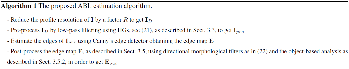
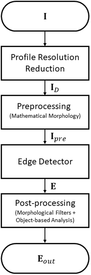
Figure 1 depicts the flowchart of the proposed MIPA approach. Instead, Algorithm 1 summarizes the sequence of the adopted signal processing steps in order to provide to the readers a complete overview of the proposed approach.
This section describes the results obtained by applying the ABL detection algorithms detailed in the previous sections on several high-resolution total attenuated backscatter lidar time series. In particular, as we use the aerosol as a proxy to determine the ABLH, we considered observations at a longer wavelength (1064 nm) to get a higher contrast among the particle and molecular contribution. In order to show the robustness of the proposed methodology, we selected different case studies characterized by different atmospheric conditions in terms of both aerosol loading and solar background. Further, we applied MIPA on observations from two quite different multi-wavelength sensors operating in different sites in terms of topography: the Potenza lidar system (MUSA) and the Évora lidar system (PAOLI).
MUSA is one of the reference lidar systems in the frame of EARLINET deployed at CNR-IMAA Atmospheric Observatory (CIAO) in Potenza (40.60∘ N, 15.72∘ E, 760 m a.s.l.). The lidar instrument is equipped with three elastic channels at 355, 532 and 1064 nm and two anelastic N2 Raman channels at 387 and 607 nm (Madonna et al., 2011). Two independent polarization components of the elastic channel at 532 nm are separately detected in order to measure the particle depolarization ratio (Freudenthaler, 2016). All channels have a raw vertical resolution of 3.75 m, and, except for the 1064 nm where only analog detection is used, all the channels are acquired both in analog and photon-counting mode to enhance the detectable dynamic range. The typical raw time resolution is 60 s. The full overlap height of the MUSA lidar is around 250–300 m.
PAOLI is the Évora EARLINET lidar system (38.57∘ N, −7.91∘ E; 293 m a.s.l.) and it operates three elastic channels (at 355, 532 and 1064 nm) and two anelastic channels at 387 and 607 nm (Althausen et al., 2009). The total and the cross-polarization channels at 532 nm are detected separately. Only photon-counting detection mode is used for all the channels. The raw vertical resolution is 30 m and the time resolution is 30 s. The full overlap height of the PAOLI system is around 750–800 m.
Even if MUSA and PAOLI operate at the same wavelengths, their technical characteristics are very different: laser source, telescope, detection and acquisition system, space and time resolution, full overlap region. Moreover, the two lidars operate in locations that from topographic point of view are quite different one from the other. As a consequence, applying the MIPA algorithm on both systems is a good benchmark to evaluate the algorithm performance.
The MIPA algorithm uses as input the composite plot of the vertically resolved attenuated backscattering coefficient at 1064 nm. High spatial and temporal resolution is needed to increase sensibility in using the directional morphological filter, while long and continuous time series are needed to improve the accuracy in mapping the detected edges. The proposed case studies are continuous multi-day observations from MUSA and PAOLI lidar systems. In July 2012, during the EARLINET 72 h exercise (Sicard et al., 2015), both Évora and Potenza EARLINET lidar stations performed continuous measurements during 72 h as proof of concept to demonstrate that EARLINET lidar network can provide aerosol optical products in near-real time (NRT) as an operational service. The observations were automatically analyzed in NRT by the EARLINET single calculus chain (SCC) (D'Amico et al., 2015), a common algorithm developed to centrally analyze and retrieve aerosol optical, geometrical and microphysical properties from the different EARLINET lidar instruments. The results obtained by applying the ABLH detection algorithm on both Potenza and Évora 72 h datasets are described in Sect. 4.1. Additionally, we selected three Potenza cases described in Sect. 4.2.
The total attenuated backscatter can be easily expressed in terms of measured lidar signals taking into account Eqs. (1) and (2):
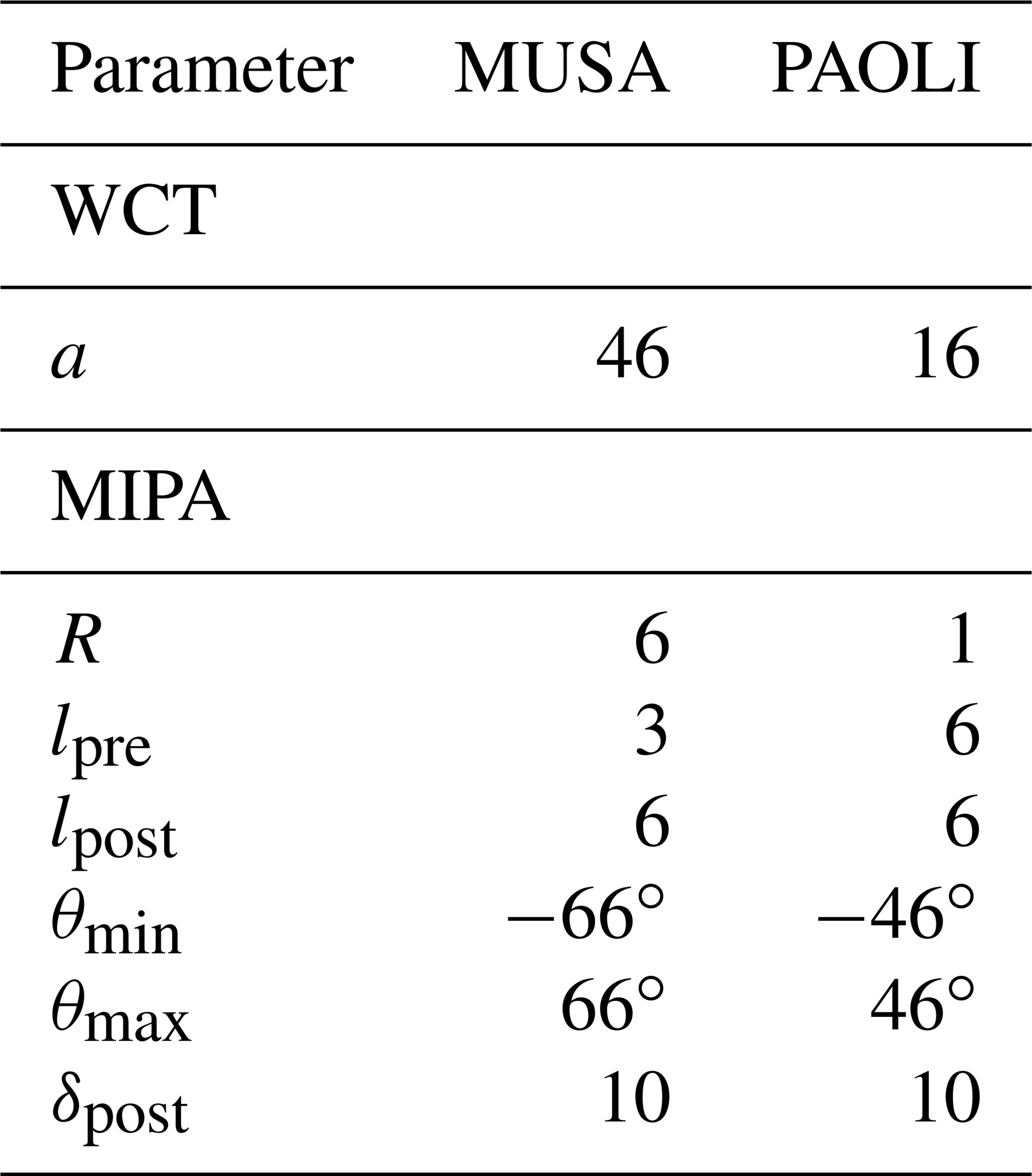
where K is a calibration constant determined by imposing that in an aerosol-free atmospheric region. It is important to note that morphological filter techniques rely only on the correlation among adjacent lidar range bin and not on their absolute numeric values. As a consequence, the ABLHs computed by the proposed MIPA algorithm are rather insensitive to the accuracy of the calibration constant K. Actually, the morphological algorithm can be applied to the range-corrected signal (Prcs) time series instead of the total attenuated backscatter one, providing the same results in terms of ABLH. This is in general not true for the traditional ABLH retrieval algorithms (derivative, WCT) where proper thresholds on absolute signal value need to be defined. Table 1 summarizes all the input parameters exploited by the compared approaches for the two lidar systems considered. These have been defined after a tuning phase on different lidar scenarios. It is worth remarking that the derivative approach requires no parameter to be set working on datasets at full resolution (60 s and 3.75 m for MUSA, 30 s and 30 m for PAOLI).
Table 1Parameter setting for the WCT and MIPA approaches. The values of the parameters can be different for different lidar systems. Thus, they are reported for both the MUSA (Potenza) and PAOLI (Évora) lidar systems.
All the input datasets considered in the study have been previously pre-processed at high resolution by using the EARLINET SCC. In particular, starting from raw lidar data, several instrumental corrections (for example, trigger delay correction, dead-time correction, analog and photon-counting signal gluing) and all the required raw signal handling (like atmospheric background subtraction, range correction) have been applied. More details on the pre-processing procedure implemented in the EARLINET SCC are described in D'Amico et al. (2016).
To assess the performance of all the considered ABLH retrievals, a reference needs to be set. As the most rigorous definition of the ABL is the one based on thermodynamic effects, we assume as reference for the ABLH the values retrieved from atmospheric temperature and pressure profiles. In particular, the reference ABLHs described in Liu and Liang (2010) are derived by applying potential temperature defined as
where θ(z) is the potential temperature that is function of the vertical height, z, Ps0 is the atmospheric pressure at the reference level of 1000 hPa, T(z) is the temperature in Kelvin, and Ps(z) is the pressure that is a function of z and k=0.286. The temperature and pressure data are obtained from ECMWF models. It is important to note that, in general, the thermodynamic definition of the ABL is different from the one typically adopted in lidar-based observations, where the atmospheric aerosol is assumed to act as an ABL tracer. During daytime conditions, the two definitions are typically equivalent: the ABL is well developed from a thermodynamic point of view, and most of the aerosols are well mixed and trapped in it. During nighttime conditions, ABL can be composed of stable and residual layers. Consequently, the ABLH retrieved assuming the thermodynamic or the lidar-based ABL definition can differ providing, in one case, the top of the stable and, in the other case, the top of the residual layer. In this context, it is worth underlining that the definition of the ABLH based on aerosol content (the one commonly used in the lidar community) is somehow ambiguous because it is mainly based on the retrieval of the first (from the surface) edge in the profile of the lidar variable proportional to the aerosol content. How this edge is attributed to a specific internal ABL sublayer cannot be determined without additional information such as turbulence or temperature.
The the number of sounding data available for all the measurement dates considered in this study is quite limited, and with the exception of one case, they are not co-located with the lidar station. In particular, there are no sounding data available for Potenza for any of the 72 h exercise days. The closest sounding stations are Brindisi (40.66∘ N, 17.96∘ E; 15 m a.s.l. and located about 180 km away from Potenza EARLINET station) and Pratica di Mare (41.67∘ N, 12.45∘ E; 32 m a.s.l. located about 300 km away from Potenza EARLINET station) which are both coastal sites with very different atmospheric conditions with respect to the mountain Potenza lidar station (760 m a.s.l.). As a consequence, the corresponding temperature and pressure profiles cannot be used to retrieve a reliable ABLH reference. Only for one of the additional selected Potenza measurement cases (20 November 2014), a single radiosonde launched at CIAO observatory (Madonna et al., 2011) is available, which however provides only one reference point that is not enough to well assess the performance of the lidar-based ABLH retrieval. For the Évora EARLINET observational site, the closest sounding station is Lisboa/Gago Coutinho (38.77∘ N, −9.13∘ E; 110 m a.s.l. and located about 110 km away from the Évora EARLINET station) at noon local time daily. Even if in this case the atmospheric conditions characterizing Lisboa/Gago Coutinho sounding station could be considered similar to the ones characterizing the Évora EARLINET station, the 72 h exercise ABLH reference points obtainable by using close soundings are only three and all referring to the same hour of the day.
Because of the lack of enough co-located and simultaneous soundings to guarantee a reliable ABLH reference for both Potenza and Évora measurement sites, the performance of the ABLH retrievals based on lidar observations has been assessed comparing against the ABLH calculated using atmospheric temperature and pressure profiles as provided by the numerical weather prediction (NWP) model. To our knowledge, NWP is the best alternative to the use of sounding data. In particular, to calculate the ABLH reference points for all the Potenza cases, we have used the high-resolution NWP provided by the ECMWF Integrated Forecast System (https://www.ecmwf.int/en/forecasts, last access: 15 March 2021). We have used forecasts providing temperature and pressure profiles in correspondence of 91 model levels on a grid. The vertical resolution increases linearly starting from 20–30 m up to about 400 m below 6 km allowing quite accurate determination of the ABLH. Moreover, the forecast time resolution of 1 h ensuring the calculation of sufficient number of ABLH reference points for all the considered Potenza cases. The ABLH reference points for the Évora 72 h exercise dataset have been calculated using the forecasts provided by Global Data Assimilation System (GDAS) of the National Centers of Environmental Predictions of NOAA (https://www.ready.noaa.gov/gdas1.php, last access: 15 March 2021). In this case, the atmospheric temperature and pressure profiles are given for 23 model levels on a grid. The vertical resolution increases with the altitude starting from values of 200–300 m close to ground and reaching values of about 800 m at around 6 km. The forecast time resolution is 3 h. We used GDAS forecasts to calculate the ABLH reference for the 72 h Évora dataset because we do not have access to the corresponding ECMWF NWP. Both ECMWF and GDAS forecasts have been obtained through the CloudNET data portal (http://devcloudnet.fmi.fi, last access: 15 March 2021).
4.1 EARLINET 72 h exercise
Figure 2 shows the total attenuated backscatter time series at 1064 nm measured by the MUSA system during the 72 h EARLINET exercise (Wang et al., 2014; Sicard et al., 2015, 2016; Granados-Muñoz et al., 2016). The lidar observations started on 9 July 2012 at 08:00 UTC and went on almost continuously until 12 July 2012 08:00 UTC. The aerosol load observed during these measurements is consistent with a typical summer day in Potenza. The aerosol aloft is mainly dust, while the layer at surface (into the ABL) is typically composed of local aerosols mixed with dust. Often, the aerosols in the free troposphere tend to intrude in the ABL, making the separation between the ABL and the upper atmospheric region not so clear. This is clearly visible around noon on 10 and 11 July 2012. The general idea behind the retrieval of ABLH from lidar measurements is to use the aerosol as tracers of the ABL and assuming that the ABLH is given by the top of the first aerosol layer (starting from the surface). According to this assumption, we can clearly see that the ABLH is maximum around noon (when the solar convection is at its maximum) for all three days, and it reaches its minimum during nighttime. The black line in Fig. 2 shows the ABLH as retrieved by MIPA algorithm. In general, the expected temporal evolution of the ABLH is well captured and the intrusions of the upper aerosol layers in the ABL do not seem to affect the outcomes, thus still obtaining reasonable ABLH estimates.
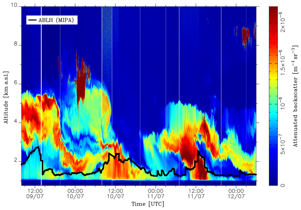
Figure 2High-resolution time series of the total attenuated backscatter at 1064 nm measured over Potenza during the EARLINET 72 h exercise (9–12 July 2012). Time resolution is 60 s, vertical resolution is 3.75 m. The black curve shows the ABLH as retrieved by the proposed MIPA algorithm.
It is important to highlight that the assumption to retrieve the ABLH as the top of the first detected aerosol layer is valid only if the ABL is above the full lidar overlap height. During nighttime observations, this condition may be not always verified, and in this case the algorithm detects as first edge the base of the layer next to the ABL top. This is clearly visible during the nighttime period in Fig. 2, where the real ABL is too low to be detected with the MUSA system and the retrieved ABLH is typically overestimated (Di Girolamo et al., 1999).
As explained in Sect. 3, the MIPA algorithm is composed of four different modules: an edge detector based on Canny filter (see Sect. 3.4), a module for reducing the vertical resolution (see Sect. 3.2), the pre-processing module described in Sect. 3.3 to be applied before the edge detector and, finally, a post-processing (see Sect. 3.5) to be applied after the edge detector step. Figure 3 shows the role played by each of these modules in retrieving the ABLH for the Potenza 72 h dataset and also the reference ABLH retrieved using the ECMWF forecasts (brown circles). The ABLHs shown in the upper panel of Fig. 3 were calculated considering the different steps of the MIPA algorithm, i.e., applying the edge detector module on full-resolution data (curve a in the upper panel of Fig. 3), the vertical resolution reduction module and the edge detector (curve b), the vertical resolution reduction module, the pre-processing module and the edge detector (curve c) and finally the whole algorithm (curve d). It is evident that the edge detector is not sufficient to ensure a stable retrieval even if it is applied to a reduced resolution dataset. Consequently, the application of the post-processing module is crucial in the processing. The absolute differences with respect to the reference are plotted in bottom panel of Fig. 3. In calculating the absolute difference, the reference data have been always interpolated at the same resolution of the lidar data assuming that the ABL is slowly varying.

Figure 3(a) ABLH retrieved during the 72 h EARLINET exercise (9–12 July 2012) for Potenza. Gray, red, yellow and black lines show the ABLH retrieved from 1064 nm high-resolution total attenuated backscatter time series by applying the edge detector module on full-resolution data (curve a), the vertical resolution reduction module and the edge detector (curve b), the vertical resolution reduction module, the pre-processing module and the edge detector (curve c) and the whole MIPA procedure (curve d). Brown circles are the reference ABLHs as retrieved from atmospheric temperature and pressure profiles provided by ECMWF forecasts. (b) Absolute differences of the retrieved ABLHs with respect to the reference. The original time resolution of ECMWF forecasts is 1 h. They have been interpolated at the lidar data time resolution (60 s).
The upper panel of Fig. 4 shows the comparison between the ABLH retrieved by the MIPA algorithm and the corresponding one obtained by using more traditional ABLH detection approaches. Specifically, we applied to the same dataset different algorithms for the ABLH estimation: the MIPA algorithm 1, the derivative method described in Sect. 2.1 and the procedure based on WCT as in Sect. 2.2. The ABLH retrieved using the ECMWF forecasts is reported as brown circles in Fig. 4. The agreement among the ABLH obtained by applying the considered algorithms on lidar data is satisfactory. The MIPA algorithm provides the smallest discrepancies with respect to the reference. In general, all the algorithms overestimate the ABLH in nighttime conditions. As already mentioned earlier, this discrepancy can be due to two main reasons: the first one is related to the different definitions we adopted to retrieve the ABLH (the ABLH reference points are based on a thermodynamic definition of the ABL, while the ABLHs retrieved from lidar observations use the atmospheric aerosol as a proxy to characterize the ABL); the second reason is due to the fact that the ABLH as retrieved by ECMWF forecasts data may be below the full overlap of the MUSA lidar.

Figure 4(a) ABLH retrieved during the 72 h EARLINET exercise (9–12 July 2012) for Potenza. Black, red and yellow lines show the ABLH retrieved from 1064 nm high-resolution total attenuated backscatter time series applying MIPA, derivative and WCT algorithms, respectively. Brown circles are the reference ABLH as retrieved from atmospheric temperature and pressure profiles provided by ECMWF forecasts. (b) Absolute differences of the retrieved ABLHs with respect to the reference. The original time resolution of ECMWF forecasts data is 1 h. They have been interpolated at the lidar data time resolution (60 s).
The absolute difference of all the considered algorithms with respect to the reference is plotted in the bottom panel of Fig. 4, and a statistical analysis is reported in Table 2 for all the considered algorithms. Both Fig. 4 and Table 2 confirm the better performance of the MIPA algorithm with respect to the other approaches into the proposed benchmark.
Table 2Statistical analysis of the absolute differences with respect to the reference of the ABLH retrieved by applying MIPA, WCT and derivative approaches on Potenza 72 h high-resolution time series of the total attenuated backscatter at 1064 nm. The mean (Δmean), the median (Δmean), the standard deviation (ΔSD), the standard error (ΔSE), the minimum and the maximum of the absolute differences are given in meters. N is the number of points on which the statistics are made. The reference is assumed to be the ABLH calculated from the co-located atmospheric temperature and pressure profiles provided by ECMWF forecasts.
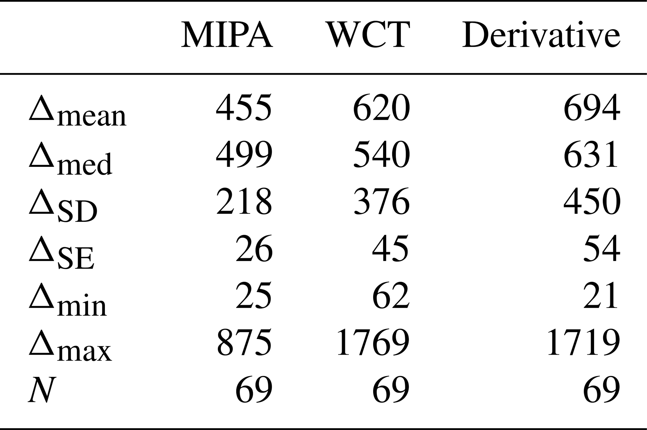
Figure 5 reports the lidar observations at 1064 nm made by PAOLI over the Évora site during the 72 h EARLINET exercise. Differently from Potenza, there are not lofted aerosol layers in the atmosphere and most of the aerosol load is trapped in the ABL. The typical evolution of the ABL due to solar activity is clearly visible in the plot. Moreover, sometimes there are small convective clouds formed on the top of ABL (see, for example, around 06:00 UTC of 11 July). The MIPA algorithm captures quite well the evolution of the ABLH (black line in Fig. 5).
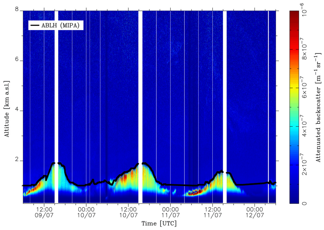
Figure 5High-resolution time series of the total attenuated backscatter at 1064 nm measured over Évora during the EARLINET 72 h exercise (9–12 July 2012). Time resolution is 30 s, vertical resolution is 30 m. The black curve shows the ABLH as retrieved by the MIPA algorithm.
Figure 6 is similar to Fig. 4 but refers to the 72 h Évora dataset. The only difference with respect to Potenza 72 h dataset is that, in this case, the reference is calculated by exploiting atmospheric temperature and pressure profiles provided by the GDAS forecasts.
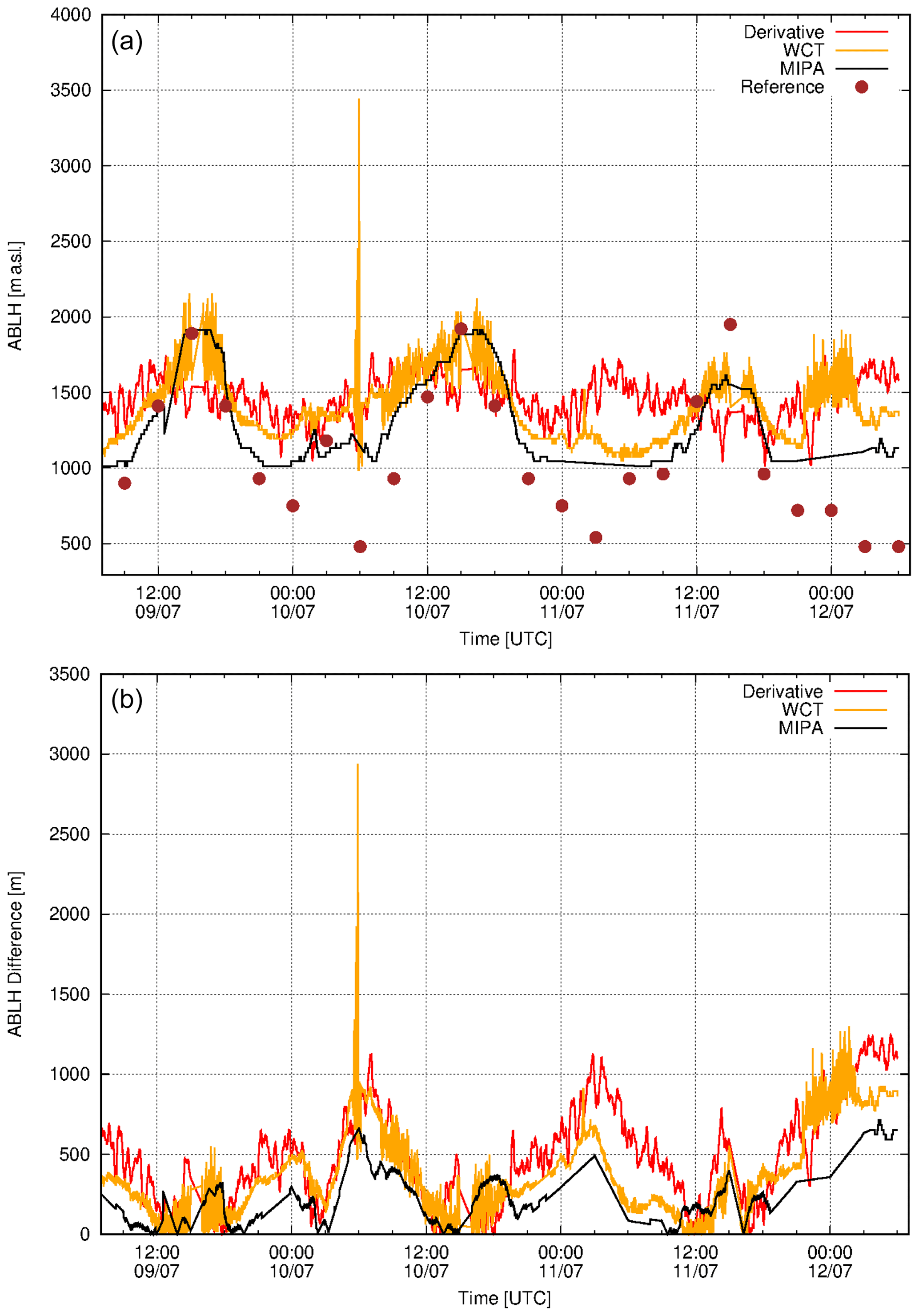
Figure 6(a) ABLH retrieved during the 72 h EARLINET exercise (9–12 July 2012) for Évora. Black, red and yellow lines show the ABLH retrieved from 1064 nm high-resolution total attenuated backscatter time series applying MIPA, derivative and WCT algorithms, respectively. Brown circles are the reference ABLHs retrieved from atmospheric temperature and pressure profiles provided by GDAS forecasts. (b) Absolute differences of the retrieved ABLHs withe respect to the reference. The original time resolution of GDAS forecasts data is 3 h. They have been interpolated at the lidar data time resolution (30 s).
Table 3 sums up the statistical analysis of the absolute differences with respect to the reference for all the considered algorithms for the 72 h Évora dataset. As for Potenza, the better performance is the one corresponding to the proposed ABLH retrieval algorithm. It is worth underlining that during daytime there is quite a good agreement between the GDAS forecasts and the outcomes of the MIPA approach; instead, during nighttime, the MIPA retrievals may be hindered by PAOLI's overlap for low ABLHs or overestimated in all the cases where there is a residual layer higher than the stable layer in the ABL.
4.2 Other Potenza cases
In this section, we describe three additional case studies on which the proposed MIPA algorithm has been evaluated. The three cases refer all to MUSA lidar observations during three longer continuous observations ever made over Potenza with MUSA.
The first case study refers to 21 April 2010 when the Potenza EARLINET station performed a quite long record of lidar measurement concurrently with the eruption of the Icelandic volcano Eyjafjallajökull occurred in April–May 2010. During the eruption, almost all the EARLINET stations promptly started continuous measurements whenever weather conditions allowed it, and the corresponding outcomes are described by Pappalardo et al. (2013).
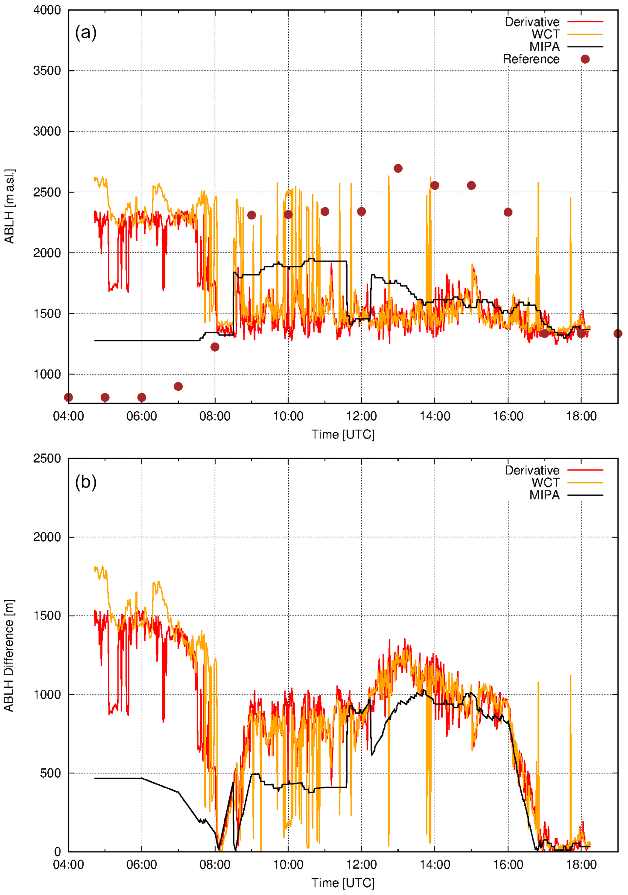
Figure 7(a) ABLH retrieved from the Potenza lidar measurements on 21 April 2010. Black, red and yellow lines show the ABLH retrieved from 1064 nm high-resolution total attenuated backscatter time series applying MIPA algorithm, derivative and WCT algorithms, respectively. Brown circles represent the reference ABLHs as retrieved from atmospheric temperature and pressure profiles provided by ECMWF forecasts. (b) Absolute differences of the retrieved ABLHs with respect to the reference. The original time resolution of ECMWF forecasts data is 1 h. They have been interpolated at the lidar data time resolution (60 s).
Table 3Statistical analysis of the absolute differences with respect to the reference of the ABLH retrieved by applying MIPA, WCT and derivative approaches on the Évora 72 h high-resolution time series of the total attenuated backscatter at 1064 nm. The mean (Δmean), the median (Δmean), the standard deviation (ΔSD), the standard error (ΔSE), the minimum and the maximum of the absolute differences are given in meters. N is the number of points on which the statistics are made. The reference is assumed to be the ABLH calculated from the co-located atmospheric temperature and pressure profiles provided by GDAS forecasts.
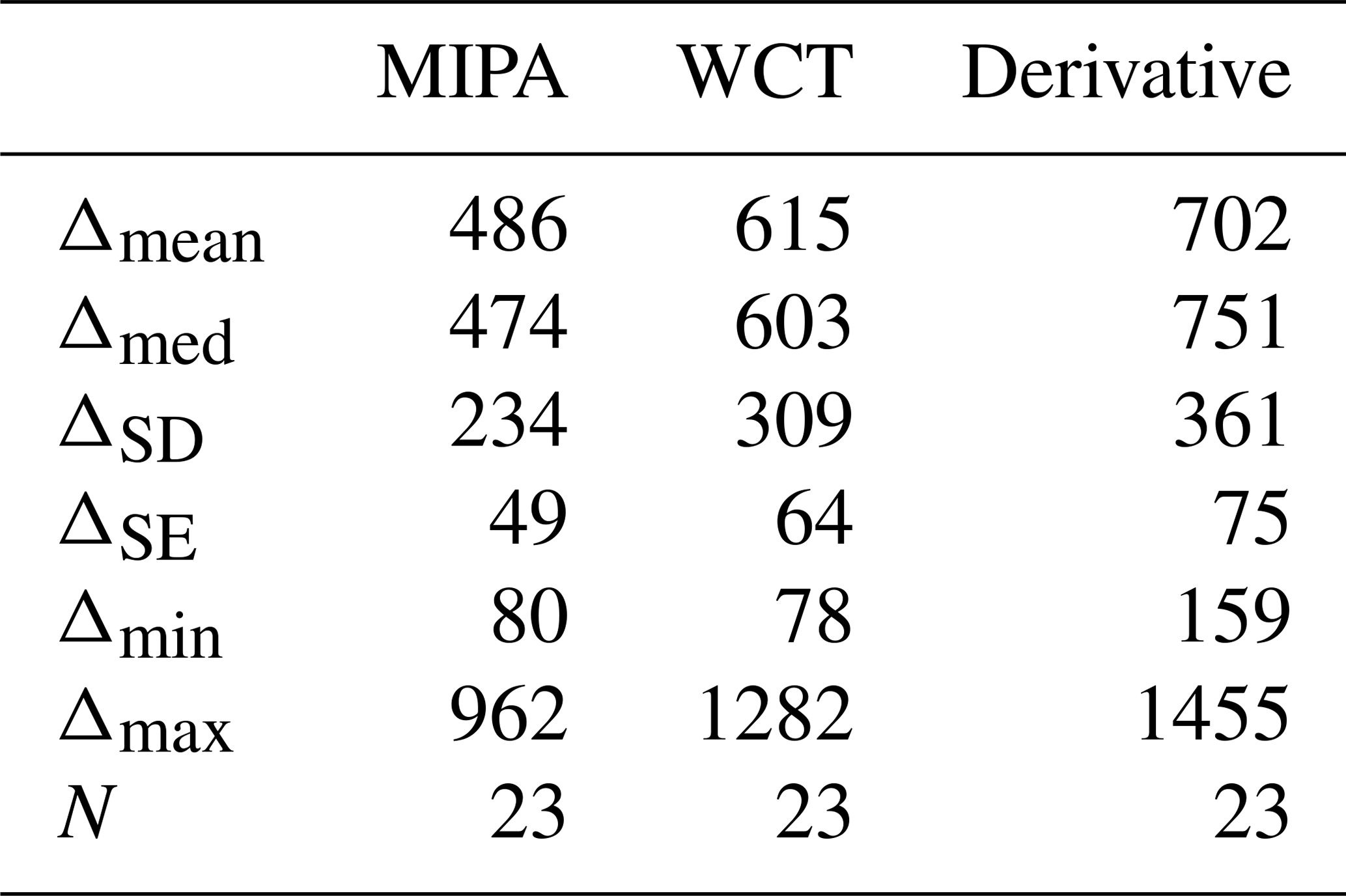
Figure 7 shows the comparison between the ABLH retrieved by the MIPA algorithm and the corresponding ABLH obtained by using the other considered algorithms (upper panel). ABLHs retrieved from ECMWF runs are assumed as reference (brown circles). The absolute difference of all the considered algorithms with respect to the reference is plotted in the bottom panel of Fig. 7. For this case, from 08:30 to 17:00 UTC, all the considered lidar retrieval algorithms give ABLH values systematically below the reference ones. This behavior can be explained by looking at Fig. 8, where the total attenuated backscatter time series at 1064 nm measured by the MUSA system on 21 April 2010 is shown. Moreover, the black line shows the ABLH retrieved by MIPA and the gray line shows the reference ABLH. Before 08:30 UTC, the real ABLH is below the MUSA overlap, and, consequently, as already mentioned earlier, the proposed algorithm overestimates the ABLH capturing the edge of the next layer. Starting from 08:30 UTC, the solar activity initiates and the ABLH starts to increase above altitudes exceeding the lidar overlap. Thus, from this point on, the ABLH retrieved by using lidar measurements should agree with the reference one. However, in this particular case, the lidar observations show that two separated aerosol layers are present below the reference ABLH (about 3 km a.s.l.) indicating that it is probably not a well-mixed ABL. The bottom layer (below about 1.5–2.0 km a.s.l.) is probably composed of local particles, while the upper one contains dust of mixed dust. Clearly, in conditions like this, the ABLH retrieved by lidar measurements (independently from the specific algorithm) will underestimate the real ABLH capturing the top of the first aerosol layer and not the top of the ABL.
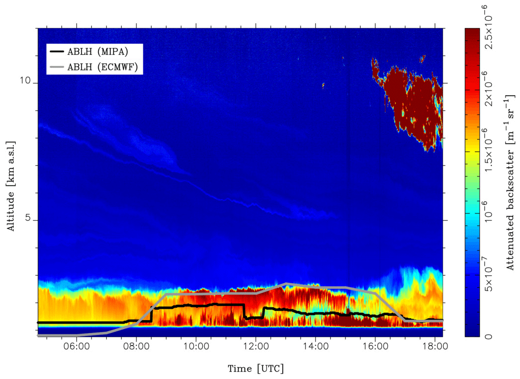
Figure 8High-resolution time series of total attenuated backscatter at 1064 nm measured over Potenza on 21 April 2010. Time resolution is 60 s; vertical resolution is 3.75 m. The black and gray curve shows the ABLH as retrieved by MIPA algorithm and by using ECMWF forecasts, respectively.
The other two cases refer to nighttime observations taken on 20 November 2014 and 13 July 2015. Figures 9 and 10 report the comparison of PBLH retrieved by all the considered algorithms (upper panel) and the absolute differences with respect to the reference (bottom panel) for the selected cases, respectively.
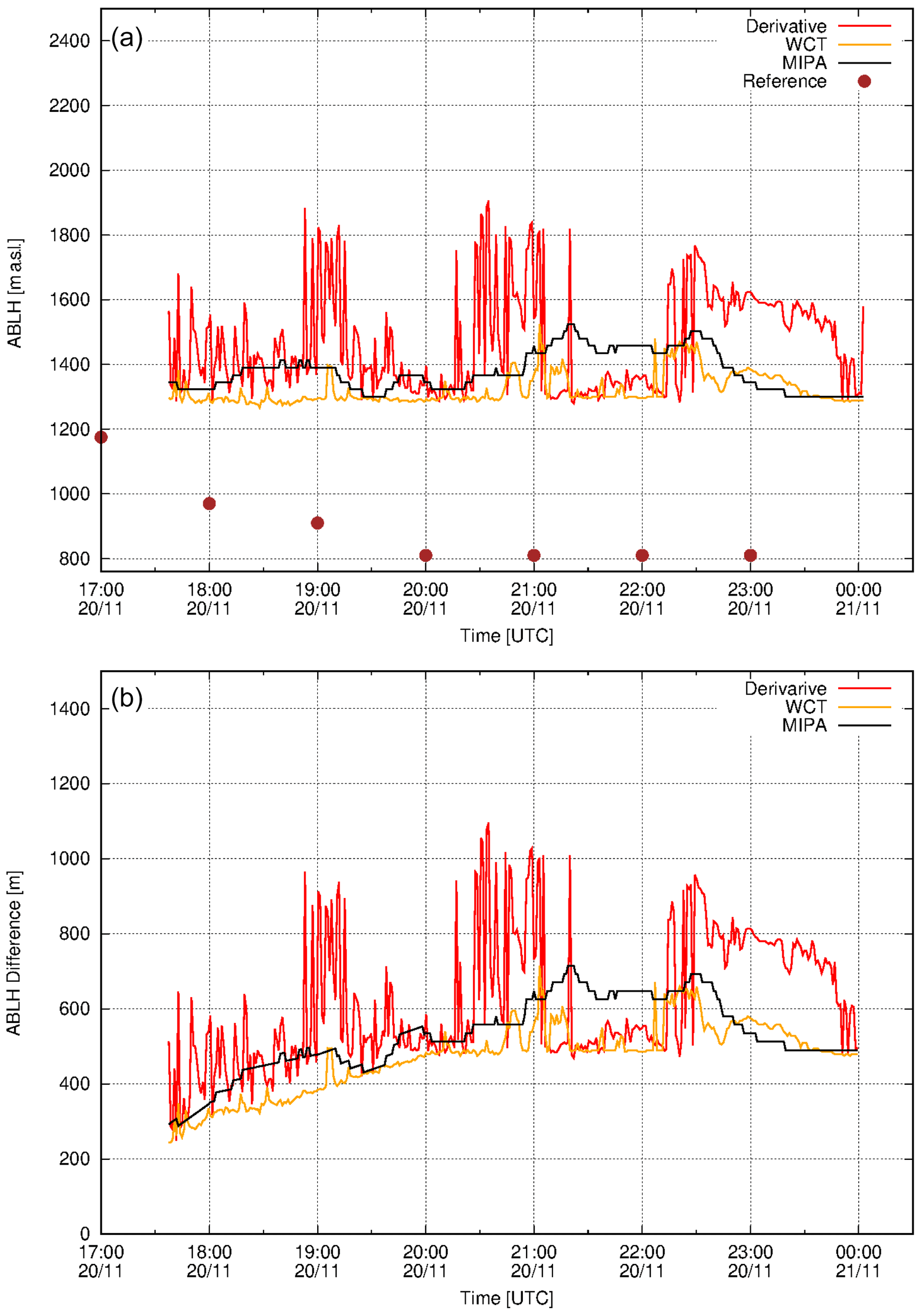
Figure 9(a) ABLH retrieved from the Potenza lidar measurements on 20 November 2014. Black, red and yellow lines show the ABLH retrieved from 1064 nm high-resolution total attenuated backscatter time series applying MIPA, derivative and WCT algorithms, respectively. Brown circles are the reference ABLHs as retrieved from atmospheric temperature and pressure profiles provided by ECMWF forecasts. (b) Absolute differences between the retrieved ABLHs with respect to the reference. The original time resolution of ECMWF forecasts data is 1 h. They have been interpolated at the lidar data time resolution (60 s).
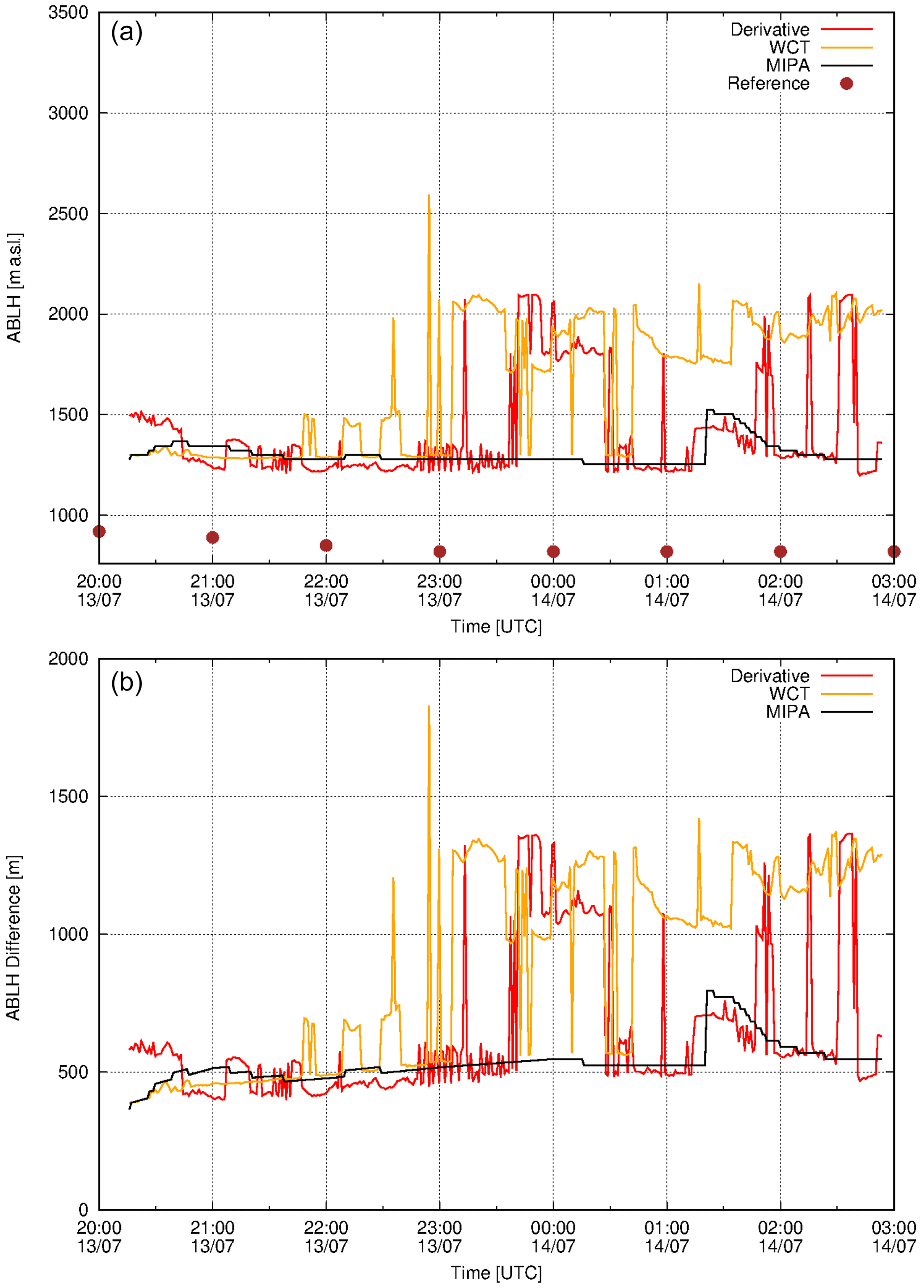
Figure 10(a) ABLH retrieved from the Potenza lidar measurements on 13 July 2015. Black, red and yellow lines show the ABLH retrieved from 1064 nm high-resolution total attenuated backscatter time series applying MIPA, derivative and WCT algorithms, respectively. Brown circles are the reference ABLHs as retrieved from atmospheric temperature and pressure profiles provided by ECMWF forecasts. (b) Absolute differences between the retrieved ABLHs with respect to the reference. The original time resolution of ECMWF forecasts data is 1 h. They have been interpolated at the lidar data time resolution (60 s).
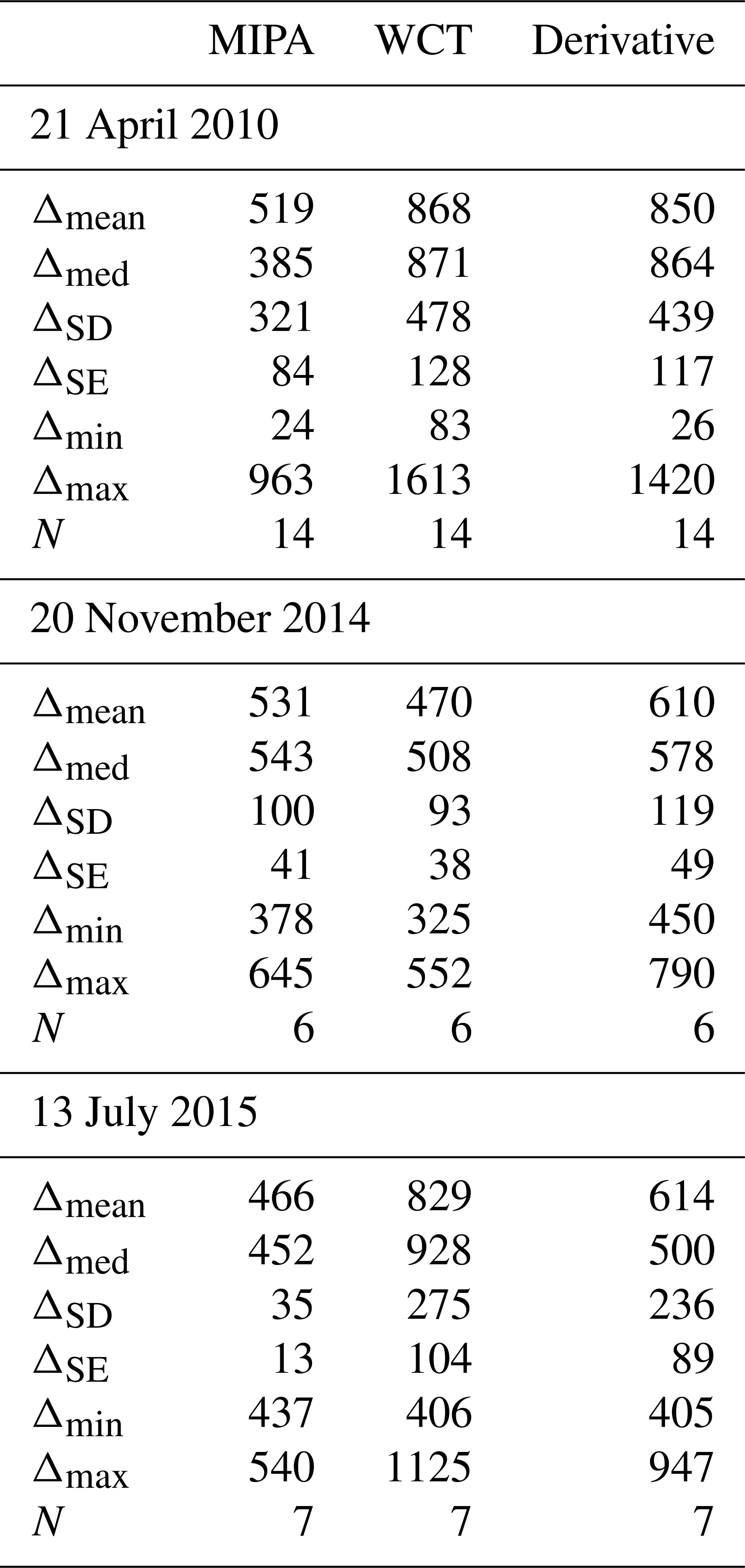
The agreement among all the considered algorithms is in general good for all the three cases. For all the cases in the dataset, the MIPA algorithm shows the highest accuracy with respect to the reference. This is confirmed also by the mean and median values of the absolute difference with respect to the reference summarized in Table 4 (minimum values of both these parameters are always obtained by using the proposed algorithm).
Table 4Statistical analysis of the absolute differences with respect to the reference of the ABLH retrieved by applying MIPA, WCT and derivative approaches on Potenza high-resolution time series of the total attenuated backscatter at 1064 nm in the three selected cases studies (21 April 2010, 20 November 2014, 13 July 2015). The mean (Δmean), the median (Δmean), the standard deviation (ΔSD), the standard error (ΔSE), the minimum and the maximum of the absolute differences are given in meters. N is the number of points on which the statistics are made. The reference is assumed to be the ABLH calculated from the co-located atmospheric temperature and pressure profiles provided by ECMWF forecasts.
The estimation of the ABLH is of crucial importance both for meteorological and air-pollution-related applications. In this work, we proposed a new algorithm to continuously retrieve the ABLH. This approach leverages the use of a fully image-based methodology (instead of analyzing the lidar observations profile by profile). The retrieval consists in applying to the image, during the pre-processing phase, morphological operators. Afterwards, an edge detection is considered. Finally, during the post-processing phase, the significant edges are extracted through a further filtering phase based on mathematical morphology and an object-based analysis. This approach has been compared with a proper benchmark consisting of state-of-the-art ABLH estimation methods, i.e., a gradient-based approach and a WCT-based method. For the latter, the filtering capabilities of the approach were pointed out. Different datasets acquired by two lidar systems located in two separated EARLINET permanent observational sites have been considered to assess the performance.
The results, relying upon several statistical indexes, put in evidence that the proposed approach is more accurate than the compared approaches belonging to the benchmark. In particular, we observed an improvement of the accuracy of about 30 % (on average) with respect to the closest state-of-the-art approach (i.e., the WCT). Moreover, the outcomes obtained by the MIPA are more stable than the other benchmarking methods. This can be easily pointed out by having a look at the results depicted in this paper, and it has also been corroborated by calculating measures of dispersion (e.g., the standard deviation) in the statistical analysis. The last concluding remark is about the computation analysis. Despite the proposed approach seeming quite complex, it leverages the use of very efficient filters based on mathematical morphology. The running times on large datasets (72 h) show excellent performance from this point of view, requiring just a few seconds for the execution of the whole signal processing chain. The bottleneck of the system turns out to be the object analysis phase. However, the computation times can be considered comparable with the other approaches proposed for the benchmark.
Finally, it is worth stressing that the MIPA approach does not depend on the absolute calibrated values but rather only on the correlation among adjacent lidar range bins, which is of crucial importance in order to form the image. This interesting feature could be very useful for future developments. Indeed, the MIPA approach could be easily adapted to address the task of the estimation of the ABLH using other widely available and continuously acquired data, such as, ceilometer data.
The developed code in MATLAB is available upon request. Once the stand-alone version is available, the software will be publicly available.
The lidar data are publicly available (upon registration) at https://actris.nilu.no/ (last access: 15 March 2021) (ACTRiS, 2021). The radiosonde data are available at http://weather.uwyo.edu/upperair/sounding.html (last access: 15 March 2021) (University of Wyoming, 2021). Radiosondes from Potenza – IMAA and Evora – ICT are available upon request.
GV and SL conceptualized the algorithm. GV developed the methodology and did the formal analysis. GV, GDA and DS validated the algorithm. GDA, AA and DB provided lidar, radiosounding and model data. GV, SL, GDA and DS took part in the process of the manuscript preparation. All authors reviewed and edited the draft. GP and GDA supervised the project. GP administered the project and acquired funds.
The authors declare that they have no conflict of interest.
This article is part of the special issue “EARLINET aerosol profiling: contributions to atmospheric and climate research”. It is not associated with a conference.
ACTRIS (https://www.actris.eu/, last access: 15 March 2021) has received funding from the European Union's Horizon 2020 research and innovation program under grant agreement nos. 654109 (ACTRIS-2), 759530 (ACTRIS-PPP), 871115 (ACTRIS-IMP) and 824068 (ENVRI-FAIR), and previously from the European Union Seventh Framework Programme (FP7/2007-2013) under grant agreement no. 262254. The Portuguese lidar station is also supported by national funds through FCT – Foundation for Science and Technology, I. P., within the scope of projects UIDB/04683/2020 and UIDP/04683/2020, and also through project TOMAQAPA (PTDC/CTAMET/29678/2017). Moreover, the authors gratefully acknowledge CloudNET for providing ECMWF and GDAS atmospheric forecasts for all the measurement cases included in this study.
This research received financial support from the European Union's Horizon 2020 research and innovation programme (grant agreement no. 654109 – ACTRIS-2 (Aerosols, Clouds, and Trace Gases Research InfraStructure)).
This paper was edited by Eduardo Landulfo and reviewed by two anonymous referees.
ACTRiS Data Centre: https://actris.nilu.no/, last access: 15 March 2021. a
Althausen, D., Engelmann, R., Baars, H., Heese, B., Ansmann, A., Müller, D., and Komppula, M.: Portable Raman Lidar PollyXT for Automated Profiling of Aerosol Backscatter, Extinction, and Depolarization, J. Atmos. Ocean. Tech., 26, 2366–2378, https://doi.org/10.1175/2009JTECHA1304.1, 2009. a
Baars, H., Ansmann, A., Engelmann, R., and Althausen, D.: Continuous monitoring of the boundary-layer top with lidar, Atmos. Chem. Phys., 8, 7281–7296, https://doi.org/10.5194/acp-8-7281-2008, 2008. a, b, c, d
Boers, R., Eloranta, E., and Coulter, R.: Lidar observations of mixed layer dynamics: Tests of parameterized entrainment models of mixed layer growth rate, J. Appl. Meteorol. Clim., 23, 247–266, 1984. a
Bösenberg, J., Hoff, R., Ansmann, A., Müller, D., Antuña, J. C., Whiteman, D., Sugimoto, N., Apituley, A., Hardesty, M., Welton, J., Eloranta, E., Arshinov, Y., Kinne, S., and Freudenthaler, V.: GAW Report No. 178: Plan for the implementation of the GAW Aerosol Lidar Observation Network GALION, Tech. rep., World Meteorological Organization, Geneva, available at: ftp://ftp.wmo.int/Documents/PublicWeb/arep/gaw/gaw178-galion-27-Oct.pdf (last access: 15 March 2021), 2008. a
Bracewell, R. N. and Bracewell, R. N.: The Fourier transform and its applications, in: vol. 31999, McGraw-Hill New York, 1986. a, b
Bravo-Aranda, J. A., de Arruda Moreira, G., Navas-Guzmán, F., Granados-Muñoz, M. J., Guerrero-Rascado, J. L., Pozo-Vázquez, D., Arbizu-Barrena, C., Olmo Reyes, F. J., Mallet, M., and Alados Arboledas, L.: A new methodology for PBL height estimations based on lidar depolarization measurements: analysis and comparison against MWR and WRF model-based results, Atmos. Chem. Phys., 17, 6839–6851, https://doi.org/10.5194/acp-17-6839-2017, 2017. a
Brooks, I.: Finding boundary layer top: application of a wavelet covariance transform to lidar backscatter profiles, J. Atmos. Ocean. Tech., 20, 1092–1105, 2003. a
Canny, J.: A computational approach to edge detection, IEEE Trans. Pattern Anal. Mach. Intel., PAMI-8, 679–698, 1986. a, b
Canut, G., Lothon, M., Saïd, F., and Lohou, F.: Observation of entrainment at the interface between monsoon flow and the Saharan Air Layer, Q. J. Roy. Meteorol. Soc., 136, 34–46, 2010. a
Cimini, D., Haeffelin, M., Kotthaus, S., Löhnert, U., Martinet, P., O'Connor, E., Walden, C., Coen, M. C., and Preissler, J.: Towards the profiling of the atmospheric boundary layer at European scale – introducing the COST Action PROBE, Bull. Atmos. Sci. Technol., 1, 23–42, 2020. a
Cohn, S. A. and Angevine, W. M.: Boundary layer height and entrainment zone thickness measured by lidars and wind-profiling radars, J. Appl. Meteorol., 39, 1233–1247, 2000. a
Comerón, A., Sicard, M., and Rocadenbosch, F.: Wavelet correlation transform method and gradient method to determine aerosol layering from lidar returns: some comments, J. Atmos. Ocean. Tech., 30, 1189–1193, 2013. a
Compton, J. C., Delgado, R., Berkoff, T. A., and Hoff, R. M.: Determination of planetary boundary layer height on short spatial and temporal scales: a demonstration of the covariance wavelet transform in ground-based wind profiler and lidar measurements, J. Atmos. Ocean. Tech., 30, 1566–1575, 2013. a
D'Amico, G., Amodeo, A., Baars, H., Binietoglou, I., Freudenthaler, V., Mattis, I., Wandinger, U., and Pappalardo, G.: EARLINET Single Calculus Chain –overview on methodology and strategy, Atmos. Meas. Tech., 8, 4891–4916, https://doi.org/10.5194/amt-8-4891-2015, 2015. a
D'Amico, G., Amodeo, A., Mattis, I., Freudenthaler, V., and Pappalardo, G.: EARLINET Single Calculus Chain – technical – Part 1: Pre-processing of raw lidar data, Atmos. Meas. Tech., 9, 491–507, https://doi.org/10.5194/amt-9-491-2016, 2016. a
Dang, R., Yang, Y., Hu, X.-M., Wang, Z., and Zhang, S.: A review of techniques for diagnosing the atmospheric boundary layer height (ABLH) using aerosol lidar data, Remote Sens., 11, 1590, https://doi.org/10.3390/rs11131590, 2019. a
Davis, K. J., Gamage, N., Hagelberg, C., Kiemle, C., Lenschow, D., and Sullivan, P.: An objective method for deriving atmospheric structure from airborne lidar observations, J. Atmos. Ocean. Tech., 17, 1455–1468, 2000. a
de Bruine, M., Apituley, A., Donovan, D. P., Klein Baltink, H., and de Haij, M. J.: Pathfinder: applying graph theory to consistent tracking of daytime mixed layer height with backscatter lidar, Atmos. Meas. Tech., 10, 1893–1909, https://doi.org/10.5194/amt-10-1893-2017, 2017. a
Di Girolamo, P., Ambrico, P. F., Amodeo, A., Boselli, A., Pappalardo, G., and Spinelli, N.: Aerosol Observations by Lidar in the Nocturnal Boundary Layer, Appl. Optics, 38, 4585–4595, 1999. a, b
Dionisi, D., Barnaba, F., Diémoz, H., Di Liberto, L., and Gobbi, G. P.: A multiwavelength numerical model in support of quantitative retrievals of aerosol properties from automated lidar ceilometers and test applications for AOT and PM10 estimation, Atmos. Meas. Tech., 11, 6013–6042, https://doi.org/10.5194/amt-11-6013-2018, 2018. a
Eresmaa, N., Karppinen, A., Joffre, S. M., Räsänen, J., and Talvitie, H.: Mixing height determination by ceilometer, Atmos. Chem. Phys., 6, 1485–1493, https://doi.org/10.5194/acp-6-1485-2006, 2006. a
Flamant, C., Pelon, J., Flamant, P. H., and Durand, P.: Lidar determination of the entrainment zone thickness at the top of the unstable marine atmospheric boundary layer, Bound.-Lay. Meteorol., 83, 247–284, 1997. a
Freudenthaler, V.: About the effects of polarising optics on lidar signals and the Δ90 calibration, Atmos. Meas. Tech., 9, 4181–4255, https://doi.org/10.5194/amt-9-4181-2016, 2016. a
Granados-Muñoz, M., Navas-Guzmán, F., Bravo-Aranda, J., Guerrero-Rascado, J., Lyamani, H., Fernández-Gálvez, J., and Alados-Arboledas, L.: Automatic determination of the planetary boundary layer height using lidar: One-year analysis over southeastern Spain, J. Geophys. Res.-Atmos., 117, 1–10, https://doi.org/10.1029/2012JD017524, 2012. a
Granados-Muñoz, M. J., Navas-Guzmán, F., Guerrero-Rascado, J. L., Bravo-Aranda, J. A., Binietoglou, I., Pereira, S. N., Basart, S., Baldasano, J. M., Belegante, L., Chaikovsky, A., Comerón, A., D'Amico, G., Dubovik, O., Ilic, L., Kokkalis, P., Muñoz Porcar, C., Nickovic, S., Nicolae, D., Olmo, F. J., Papayannis, A., Pappalardo, G., Rodríguez, A., Schepanski, K., Sicard, M., Vukovic, A., Wandinger, U., Dulac, F., and Alados-Arboledas, L.: Profiling of aerosol microphysical properties at several EARLINET/AERONET sites during the July 2012 ChArMEx/EMEP campaign, Atmos. Chem. Phys., 16, 7043–7066, https://doi.org/10.5194/acp-16-7043-2016, 2016. a
Haeffelin, M., Angelini, F., Morille, Y., Martucci, G., Frey, S., Gobbi, G., Lolli, S., O'dowd, C., Sauvage, L., Xueref-Rémy, I., Wastine, B., and Feist, D.: Evaluation of mixing-height retrievals from automatic profiling lidars and ceilometers in view of future integrated networks in Europe, Bound.-Lay. Meteorol., 143, 49–75, 2012. a
He, Q., Mao, J., Chen, J., and Hu, Y.: Observational and modeling studies of urban atmospheric boundary-layer height and its evolution mechanisms, Atmos. Environ., 40, 1064–1077, 2006. a
Hooper, W. P. and Eloranta, E. W.: Lidar measurements of wind in the planetary boundary layer: the method, accuracy and results from joint measurements with radiosonde and kytoon, J. Clim. Appl. Meteorol., 25, 990–1001, 1986. a
Lewis, J. R., Welton, E. J., Molod, A. M., and Joseph, E.: Improved boundary layer depth retrievals from MPLNET, J. Geophys. Res.-Atmos., 118, 9870–9879, 2013. a
Liu, S. and Liang, X.-Z.: Observed diurnal cycle climatology of planetary boundary layer height, J. Climate, 23, 5790–5809, 2010. a
Lolli, S., Delaval, A., Loth, C., Garnier, A., and Flamant, P. H.: 0.355-micrometer direct detection wind lidar under testing during a field campaign in consideration of ESA's ADM-Aeolus mission, Atmos. Meas. Tech., 6, 3349–3358, https://doi.org/10.5194/amt-6-3349-2013, 2013. a
Lolli, S., Khor, W. Y., Matjafri, M. Z., and Lim, H. S.: Monsoon Season Quantitative Assessment of Biomass Burning Clear-Sky Aerosol Radiative Effect at Surface by Ground-Based Lidar Observations in Pulau Pinang, Malaysia in 2014, Remote Sens., 11, 2660, https://doi.org/10.3390/rs11222660, 2019. a
Lyamani, H., Fernández-Gálvez, J., Pérez-Ramírez, D., Valenzuela, A., Antón, M., Alados, I., Titos, G., Olmo, F., and Alados-Arboledas, L.: Aerosol properties over two urban sites in South Spain during an extended stagnation episode in winter season, Atmos. Environ., 62, 424–432, 2012. a
Madonna, F., Amodeo, A., Boselli, A., Cornacchia, C., Cuomo, V., D'Amico, G., Giunta, A., Mona, L., and Pappalardo, G.: CIAO: the CNR-IMAA advanced observatory for atmospheric research, Atmos. Meas. Tech., 4, 1191–1208, https://doi.org/10.5194/amt-4-1191-2011, 2011. a, b
Mahrt, L.: Stratified atmospheric boundary layers, Bound.-Lay. Meteorol., 90, 375–396, 1999. a, b
Melfi, S., Spinhirne, J., Chou, S.-H., and Palm, S.: Lidar observations of vertically organized convection in the planetary boundary layer over the ocean, J. Clim. Appl. Meteorol., 24, 806–821, 1985. a
Menut, L., Flamant, C., Pelon, J., and Flamant, P. H.: Urban boundary-layer height determination from lidar measurements over the Paris area, Appl. Optics, 38, 945–954, 1999. a
Morille, Y., Haeffelin, M., Drobinski, P., and Pelon, J.: STRAT: An automated algorithm to retrieve the vertical structure of the atmosphere from single-channel lidar data, J. Atmos. Ocean. Tech., 24, 761–775, 2007. a
Pappalardo, G., Mona, L., D'Amico, G., Wandinger, U., Adam, M., Amodeo, A., Ansmann, A., Apituley, A., Alados Arboledas, L., Balis, D., Boselli, A., Bravo-Aranda, J. A., Chaikovsky, A., Comeron, A., Cuesta, J., De Tomasi, F., Freudenthaler, V., Gausa, M., Giannakaki, E., Giehl, H., Giunta, A., Grigorov, I., Groß, S., Haeffelin, M., Hiebsch, A., Iarlori, M., Lange, D., Linné, H., Madonna, F., Mattis, I., Mamouri, R.-E., McAuliffe, M. A. P., Mitev, V., Molero, F., Navas-Guzman, F., Nicolae, D., Papayannis, A., Perrone, M. R., Pietras, C., Pietruczuk, A., Pisani, G., Preißler, J., Pujadas, M., Rizi, V., Ruth, A. A., Schmidt, J., Schnell, F., Seifert, P., Serikov, I., Sicard, M., Simeonov, V., Spinelli, N., Stebel, K., Tesche, M., Trickl, T., Wang, X., Wagner, F., Wiegner, M., and Wilson, K. M.: Four-dimensional distribution of the 2010 Eyjafjallajökull volcanic cloud over Europe observed by EARLINET, Atmos. Chem. Phys., 13, 4429–4450, https://doi.org/10.5194/acp-13-4429-2013, 2013. a
Pappalardo, G., Amodeo, A., Apituley, A., Comeron, A., Freudenthaler, V., Linné, H., Ansmann, A., Bösenberg, J., D'Amico, G., Mattis, I., Mona, L., Wandinger, U., Amiridis, V., Alados-Arboledas, L., Nicolae, D., and Wiegner, M.: EARLINET: towards an advanced sustainable European aerosol lidar network, Atmos. Meas. Tech., 7, 2389–2409, https://doi.org/10.5194/amt-7-2389-2014, 2014. a
Sailor, D. J.: Simulated urban climate response to modifications in surface albedo and vegetative cover, J. Appl. Meteorol., 34, 1694–1704, 1995. a
Sicard, M., Pérez, C., Rocadenbosch, F., Baldasano, J., and García-Vizcaino, D.: Mixed-layer depth determination in the Barcelona coastal area from regular lidar measurements: methods, results and limitations, Bound.-Lay. Meteorol., 119, 135–157, 2006. a
Sicard, M., D'Amico, G., Comerón, A., Mona, L., Alados-Arboledas, L., Amodeo, A., Baars, H., Baldasano, J. M., Belegante, L., Binietoglou, I., Bravo-Aranda, J. A., Fernández, A. J., Fréville, P., García-Vizcaíno, D., Giunta, A., Granados-Muñoz, M. J., Guerrero-Rascado, J. L., Hadjimitsis, D., Haefele, A., Hervo, M., Iarlori, M., Kokkalis, P., Lange, D., Mamouri, R. E., Mattis, I., Molero, F., Montoux, N., Muñoz, A., Muñoz Porcar, C., Navas-Guzmán, F., Nicolae, D., Nisantzi, A., Papagiannopoulos, N., Papayannis, A., Pereira, S., Preißler, J., Pujadas, M., Rizi, V., Rocadenbosch, F., Sellegri, K., Simeonov, V., Tsaknakis, G., Wagner, F., and Pappalardo, G.: EARLINET: potential operationality of a research network, Atmos. Meas. Tech., 8, 4587–4613, https://doi.org/10.5194/amt-8-4587-2015, 2015. a, b
Sicard, M., Barragan, R., Muñoz Porcar, C. M., Comerón, A., Mallet, M., Dulac, F., Pelon, J., Arboledas, L. A., Amodeo, A., Boselli, A., Bravo-Aranda, J. A., D'Amico, Granados-Muñoz, M. J., Leto, G., Rascado, J. L. G., Madonna, F., Mona, L., Pappalardo, G., Perrone, M. R., Burlizzi, P., Rocadenbosch, F., Rodríguez-Gómez, A., Scollo, S., Spinelli, N., Titos, G., Wang, X., and Sanchez, R. Z.: Contribution of EARLINET/ACTRIS to the summer 2013 Special Observing Period of the ChArMEx project: monitoring of a Saharan dust event over the western and central Mediterranean, Int. J. Remote Sens., 37, 4698–4711, https://doi.org/10.1080/01431161.2016.1222102, 2016. a
Soille, P.: Morphological Image Analysis: Principles and Applications, Springer-Verlag, Berlin, Heidelberg, 2003. a, b, c, d, e
Steyn, D. G., Baldi, M., and Hoff, R.: The detection of mixed layer depth and entrainment zone thickness from lidar backscatter profiles, J. Atmos. Ocean. Tech., 16, 953–959, 1999. a
Su, T., Li, Z., and Kahn, R.: A new method to retrieve the diurnal variability of planetary boundary layer height from lidar under different thermodynamic stability conditions, Remote Sens. Environ., 237, 111519, https://doi.org/10.1016/j.rse.2019.111519, 2020. a, b
Summa, D., Di Girolamo, P., Stelitano, D., and Cacciani, M.: Characterization of the planetary boundary layer height and structure by Raman lidar: comparison of different approaches, Atmos. Meas. Tech., 6, 3515–3525, https://doi.org/10.5194/amt-6-3515-2013, 2013. a
Talianu, C., Nicolae, D., Ciuciu, J., Ciobanu, M., and Babin, V.: Planetary boundary layer height detection from LIDAR measurements, J. Optoelect. Adv. M., 8, 243–246, 2006. a
Toledo, D., Córdoba-Jabonero, C., and Gil-Ojeda, M.: Cluster Analysis: A new approach applied to Lidar measurements for Atmospheric Boundary Layer height estimation, J. Atmos. Ocean. Tech., 31, 422–436, 2014. a
Tomás, S., Rocadenbosch, F., and Sicard, M.: Atmospheric boundary-layer height estimation by adaptive Kalman filtering of lidar data, in: Remote Sensing of Clouds and the Atmosphere XV, vol. 7827, International Society for Optics and Photonics, Prague, Czech Republic, p. 782704, 2010. a
University of Wyoming: http://weather.uwyo.edu/upperair/sounding.html, last access: 15 March 2021. a
Wang, Y., Sartelet, K. N., Bocquet, M., Chazette, P., Sicard, M., D'Amico, G., Léon, J. F., Alados-Arboledas, L., Amodeo, A., Augustin, P., Bach, J., Belegante, L., Binietoglou, I., Bush, X., Comerón, A., Delbarre, H., García-Vízcaino, D., Guerrero-Rascado, J. L., Hervo, M., Iarlori, M., Kokkalis, P., Lange, D., Molero, F., Montoux, N., Muñoz, A., Muñoz, C., Nicolae, D., Papayannis, A., Pappalardo, G., Preissler, J., Rizi, V., Rocadenbosch, F., Sellegri, K., Wagner, F., and Dulac, F.: Assimilation of lidar signals: application to aerosol forecasting in the western Mediterranean basin, Atmos. Chem. Phys., 14, 12031–12053, https://doi.org/10.5194/acp-14-12031-2014, 2014. a
Yang, T., Wang, Z., Zhang, W., Gbaguidi, A., Sugimoto, N., Wang, X., Matsui, I., and Sun, Y.: Technical note: Boundary layer height determination from lidar for improving air pollution episode modeling: development of new algorithm and evaluation, Atmos. Chem. Phys., 17, 6215–6225, https://doi.org/10.5194/acp-17-6215-2017, 2017. a