the Creative Commons Attribution 4.0 License.
the Creative Commons Attribution 4.0 License.
 | 17 Mar 2021
A comparison of long-term trends in observations and emission inventories of NOx
Elena Macdonald
Noelia Otero
Air pollution is a pressing issue that is associated with adverse effects on human health, ecosystems, and climate. Despite many years of effort to improve air quality, nitrogen dioxide (NO2) limit values are still regularly exceeded in Europe, particularly in cities and along streets. This study explores how concentrations of nitrogen oxides (NOx = NO + NO2) in European urban areas have changed over the last decades and how this relates to changes in emissions. To do so, the incremental approach was used, comparing urban increments (i.e. urban background minus rural concentrations) to total emissions, and roadside increments (i.e. urban roadside concentrations minus urban background concentrations) to traffic emissions. In total, nine European cities were assessed. The study revealed that potentially confounding factors like the impact of urban pollution at rural monitoring sites through atmospheric transport are generally negligible for NOx. The approach proves therefore particularly useful for this pollutant. The estimated urban increments all showed downward trends, and for the majority of the cities the trends aligned well with the total emissions. However, it was found that factors like a very densely populated surrounding or local emission sources in the rural area such as shipping traffic on inland waterways restrict the application of the approach for some cities. The roadside increments showed an overall very diverse picture in their absolute values and trends and also in their relation to traffic emissions. This variability and the discrepancies between roadside increments and emissions could be attributed to a combination of local influencing factors at the street level and different aspects introducing inaccuracies to the trends of the emission inventories used, including deficient emission factors. Applying the incremental approach was evaluated as useful for long-term pan-European studies, but at the same time it was found to be restricted to certain regions and cities due to data availability issues. The results also highlight that using emission inventories for the prediction of future health impacts and compliance with limit values needs to consider the distinct variability in the concentrations not only across but also within cities.
- Article
(1971 KB) - Full-text XML
-
Supplement
(116 KB) - BibTeX
- EndNote


The assessment of air quality has been of interest for many years because it is affected by human activity and simultaneously has an effect on us and our environment. Depending on the air pollutant, impacts on human health, ecosystems, and the climate have been observed (Guerreiro et al., 2014). In this study the focus is on NOx, i.e. the sum of nitric oxide (NO) and nitrogen dioxide (NO2). Even though limit values are defined for NO2, the two pollutants are often assessed as NOx due to their close chemical coupling (Carslaw and Beevers, 2005). The share of either pollutant (NO or NO2) in the total amount of NOx depends on many factors such as the initial emissions, ambient concentrations of ozone (O3), and meteorological conditions (Carslaw and Beevers, 2005; von Schneidemesser et al., 2017). Due to the close coupling of NO and NO2, emission inventories (EIs) also typically report NOx emissions (Lee et al., 2015). Like most air pollutants, NOx can have adverse effects on human health and ecosystems. Exposure to NO2, both short-term and long-term, has been associated with increases in all-cause mortality as well as with adverse effects on cardiovascular and respiratory systems (Faustini et al., 2014; Mills et al., 2015). Furthermore, NOx plays an important role in the formation of secondary pollutants such as particulate matter (PM) and O3 (Carslaw et al., 2011a; von Schneidemesser et al., 2017), which in turn are associated with adverse effects on health, ecosystems, and climate (Guerreiro et al., 2014; Richter, 2009).
In the European Union (EU), limit values for NO2 in the atmosphere have been in place since 1985 (Council of the European Union, 1985). The most recent limit values are defined in a directive from 2008 and are set to an annual mean of 40 µg m−3 and an hourly mean of 200 µg m−3 that should not be exceeded more than 18 times a year (European Parliament and Council of the European Union, 2008). These limit values are still regularly exceeded. In 2017, exceedances of the annual NO2 limit were recorded in 16 EU member states (EEA, 2019a). Urban areas are particularly affected; in 2017, 86 % of the exceedances of the annual limit value were observed at air quality monitoring stations along roads (Carslaw et al., 2011a; EEA, 2019a).
Another aspect that makes NOx a pollutant of particular interest is the discrepancy that was found between emission standards and real-world emissions from some vehicle classes (Vestreng et al., 2009). Since the 1970s, road transport has been the main source of NOx emissions, and in recent years it was found that these emissions did not decrease as expected (Vestreng et al., 2009). To reduce air pollution, so-called Euro emissions standards were introduced in the 1990s which set limits for the exhaust emissions from new vehicles (Font and Fuller, 2016). These standards have been gradually tightened over the last decades, but it was noticed that the NOx emissions under real-world driving conditions did not reduce accordingly for some vehicles (Carslaw et al., 2011a). Especially diesel vehicles were found to have higher emissions (Carslaw et al., 2011a). It was estimated that, if true on-road NOx emissions of diesel vehicles met the regulatory standards, this would result in a reduction of the overall traffic emissions in a city by 30 to 75 % (von Schneidemesser et al., 2017).
Comparing EIs to measurements can help in understanding any inadequacies and uncertainties that are related to the EIs (Beevers et al., 2012). It has been acknowledged that even though the quality of EIs improved over the last years there are still large uncertainties associated with them (Lee et al., 2015; Vestreng et al., 2009). One way of evaluating EIs through a comparison with concentration measurements is by analysing trends rather than absolute or modelled values. When long-term trends are analysed, aspects like chemistry and meteorology can be assumed negligible, and it can be assessed whether the changes in the observed ambient concentrations reflect the changes that would be expected based on the emissions (Beevers et al., 2009).
The comparison of the trends in measurements and emissions was done using the so-called incremental approach. It was first used in a study by Lenschow et al. (2002) on PM in Berlin and is therefore also referred to as the Lenschow approach (Thunis, 2018). According to the approach, the difference between urban background and rural background concentration levels of a pollutant is the urban increment, and, similarly, the difference between measurements from urban traffic sites and the urban background makes up the roadside increment. According to Lenschow et al. (2002), the urban increment can be attributed to the total emission sources of a city, and, likewise, it can be assumed that traffic emissions lead to the roadside increments (e.g. Beevers et al., 2009; von Schneidemesser et al., 2017). Following from this, it is then assumed that any changes in either of the emissions should lead to proportional changes in the related increment, again in line with the above-mentioned studies.
A major advantage of this approach is that any large-scale processes, such as meteorological conditions or the dynamics of the mixing height of the atmosphere, should not confound the analysis because they are influencing both urban and rural concentration levels (Font and Fuller, 2016). Especially variations in the meteorological conditions can either falsely emphasise or mask a trend in the concentrations, and so minimising this effect allows a better comparison with emission changes (Beevers et al., 2009). Nevertheless, there are also aspects that have been criticised about this approach. For example, Thunis (2018) and Torras Ortiz and Friedrich (2013) noted that it is assumed that the rural measurements are not impacted by urban emissions even though this can likely be the case. To what extent this affects the accuracy of urban increments was evaluated before using the approach in this study.
The incremental approach is well established for the analysis of PM but has seen less application yet for the analysis of NOx. Urban increments of PM and NO2 were for example calculated by Elser et al. (2016), Petetin et al. (2014), Pey et al. (2010), and Thunis (2018), and roadside increments of PM, NO2, and NOx were estimated for example by Beevers et al. (2009), Font et al. (2019), and von Schneidemesser et al. (2017). Those studies all focus on individual cities, e.g. Berlin (von Schneidemesser et al., 2017), or small groups of cities, e.g. London and Paris (Font et al., 2019), and mainly assess ambient concentrations in major urban areas. Furthermore, most of the studies analyse set periods of time, such as 1 year (Elser et al., 2016), 5 years (Beevers et al., 2009), or 10 years (Font et al., 2019). In contrast to that, the study at hand attempts to apply the approach systematically to the analysis of trends in NOx across all of Europe. On one hand, this means that also smaller urban areas are included in the analysis. On the other hand, it also enhances the temporal scope to over 25 years for some cities instead of limiting it to a set time period.
The aim of this study is to examine how NOx concentrations and emissions have evolved over the last decades in European cities and how their trends relate to each other. Changes in urban and roadside increments will be compared to changes in total and traffic emission inventories to assess whether the trends align as would be expected or whether any discrepancies can be found. Furthermore, the study aspires to evaluate if the incremental approach is a useful tool for pan-European studies on NOx, especially with regards to data availability and aspects that are sometimes criticised about this approach. This was done by an examination of the data that are available for European cities, assessing the incremental approach in detail and finally applying it to the cities where the data allowed it.
Except as stated otherwise, all analyses were carried out using RStudio (RStudio Team, 2019) and R (R Core Team, 2020), along with the R packages listed in the Supplement (Table S1).
2.1 Data
The measurements of ambient NOx concentrations were obtained from the AirBase database. Observations from rural background (RB), urban background (UB), and urban traffic (UT) stations were used to calculate urban and roadside increments. From the respectively classified stations, daily NOx data were used to calculate annual averages for all years with sufficient data between 1990 and 2017. The data had to meet the following criteria, as suggested by the EEA (2009): the annual coverage of values should be at least 75 % in order to include data from the respective year, and each individual record needed to pass a visual quality screening. No minimum record length was set for urban stations.
The EIs were sourced as gridded emissions from the European Monitoring and Evaluation Programme (EMEP). The EMEP grid provides annual emission data from 1990 to 2017 in a 0.1∘ × 0.1∘ long–lat resolution in the geographic coordinate system WGS84 (Wankmueller, 2019). It is based on the national and sectoral emissions that are reported by the participating states under the Convention on Long-range Transboundary Air Pollution. Using QGIS 3.10 (QGIS Development Team, 2019) and shapefiles of the city boundaries (sources in the Supplement, Table S2), city averages of total and traffic NOx emissions per year were calculated from the gridded EIs.
Data on wind directions and wind speed were obtained for seven cities from the respective national weather services. For most cities, hourly data were available, but for two cities only three measurements per day were provided. A table listing the measuring stations that recorded the wind data as well as the temporal resolutions and time periods of the data sets can be found in the Supplement (Table S3).
2.2 Selection of cities
The selection of cities was based solely on the availability of air quality observations. A search algorithm was developed to find all cities with at least one UB and two UT stations. The cities were sorted by the record lengths of their stations, and the ones with promising data availability were subject to a visual inspection of the continuity and consistency of the annual data of all respective UB and UT stations. The resulting preselection of cities was analysed for the availability of rural stations in their surroundings. For the RB, long records from single stations were not considered as important as for the other two station types, but rather throughout the whole time period any station provides data. This led to a final selection of cities (see Sect. 3.1) that seemed suitable for the planned analysis.
2.3 Calculation of increments
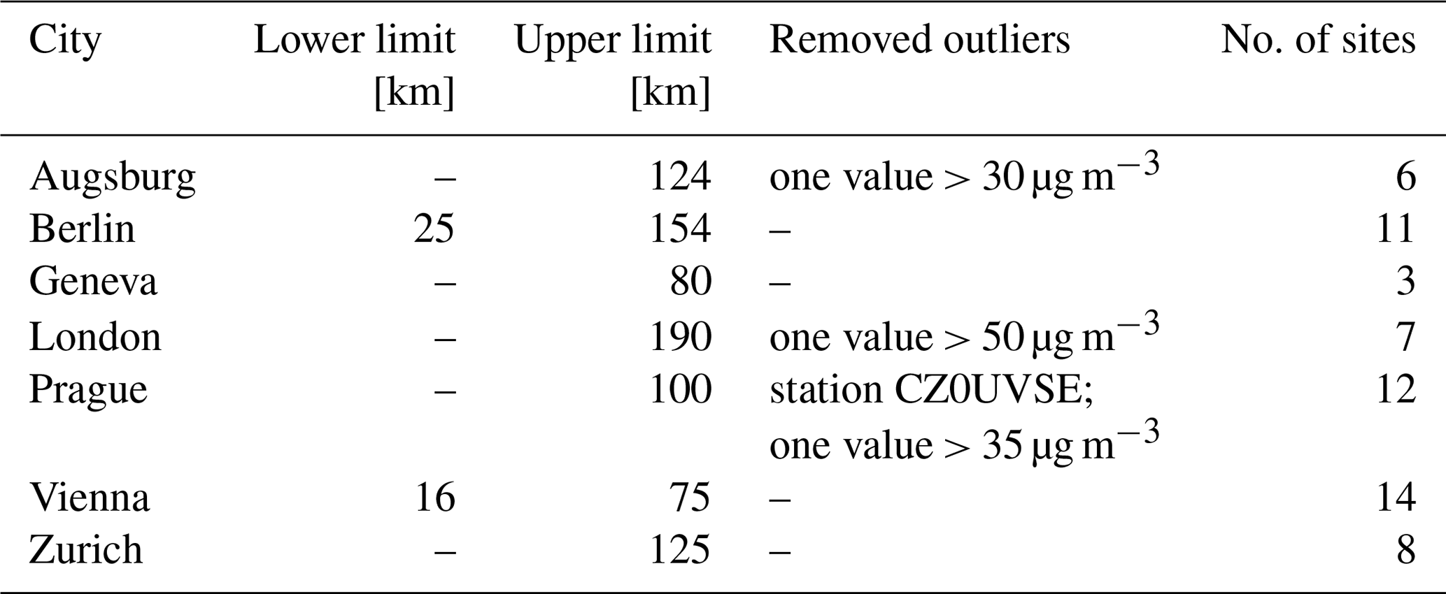
To analyse the air quality observations, increments were calculated based on annual averages derived from daily data. The urban increment was set as the difference between the UB concentration and the RB concentration (e.g. Lenschow et al., 2002; Thunis, 2018; Torras Ortiz and Friedrich, 2013). Similarly, the roadside increment was defined as the UT concentration minus the UB concentration (e.g. Beevers et al., 2009; Font et al., 2019; von Schneidemesser et al., 2017). While the data of each UT station were used individually to calculate roadside increments, one representative urban as well as rural background concentration was established for each city. For the UB concentration this was done by averaging the annual data of all UB stations in a city. Similarly, the RB concentration was set as the average of the annual data from several RB stations. To do so, the data of all RB stations which are within a 200 km radius around a city centre and which provided data for more than 8 years was examined, and stations were selected based on their data ranges. Where the stations in the vicinity of the city showed relatively consistent concentration levels to each other, a maximum radius for including stations was defined as the distance where a deviation from the consistent level was observed. Furthermore, some stations very close to or still within a city were excluded if they showed distinctively higher values, along with some stations further away where the concentration ranges indicated a potential local influence. Where the stations in the vicinity showed no consistent level, the city was excluded from the analysis of the urban increment.
Including stations with different record lengths in the calculation of a mean RB concentration can lead to inconsistencies in the number of stations providing data per year. In some years, only very few stations may have recorded data, and, if these stations measure comparatively high (or low) concentrations, such biases in the monitoring network can introduce misleading trends in the average (Lang et al., 2019). To resolve this issue, the mean RB levels were calculated using moving window regression as suggested by Lang et al. (2019), with the window width of 3 years recommended therein.
The impact of atmospheric transport
One of the underlying assumptions of the incremental approach is that the rural background concentrations are independent of the urban concentrations. If high air pollution in the urban area led to increased concentrations in the surrounding rural area, the calculated urban increment would underestimate the contribution of the city to the total concentration level (Pey et al., 2010). Some studies note that this is likely the case and that the urban increments should therefore be regarded as minimum (Pey et al., 2010; Thunis, 2018). A way in which urban pollution might impact rural concentrations is through atmospheric transport of pollutants from the city to rural areas (Torras Ortiz and Friedrich, 2013). To examine this effect, the daily RB data were split into subsets based on wind directions.
For each of the RB stations around a city, the direction in which the city is relative to the station's location was calculated, comparable to wind directions (0–360∘). Based on (7-)hourly measurements of wind speed and wind directions, daily averages of wind directions were calculated using vector calculations as denoted by Grange (2014). Afterwards, the daily data from each RB station were filtered by wind directions and split into two subsets: the first comprised all days when the wind blew within a 30∘ range from the city to the station, and the second comprised all other days. Hereinafter, the first subset will be referred to as the “downwind days”, and the second as “upwind days”. For both subsets and each RB station, annual averages were calculated, and subsequently the data from all stations around a city were averaged to two distinct mean RB levels. These downwind and upwind concentrations were compared with each other, as well as with the RB level based on the data from all days.
3.1 Availability of observational data
The availability of monitoring stations measuring NOx shows great variability across different countries and regions of Europe. In Fig. 1 the locations of RB, UB, and UT stations which are included in the AirBase database are shown, and the sites are coloured according to the number of years for which they provide NOx data through the database. This reveals regional differences in the available number of stations as well as in the length of recorded time series. A high density of stations from all three types is found in central Europe, while in Scandinavia, the Baltic states, and Finland the numbers are rather low. In general, there are fewer rural than urban stations, and this discrepancy is especially clear for France and most eastern European countries. France also stands out when looking at the record lengths that the stations provide since practically none of them has more than 5 years of data available. Most sites providing more than 15 years of data are located in central Europe, Great Britain, and Spain. While only a fifth of all stations are RB sites, the share of sites with records of 15 years or more is much higher for this type: 26 % as opposed to 13 and 10 % for UB and UT stations, respectively. The regional differences in the data availability restrict the analysis of cities with long-term data from all three station types to certain areas in Europe. In total, nine cities were selected which are all located in central Europe and Great Britain. These are Amsterdam, Augsburg, Berlin, Geneva, Linz, London, Prague, Vienna, and Zurich.
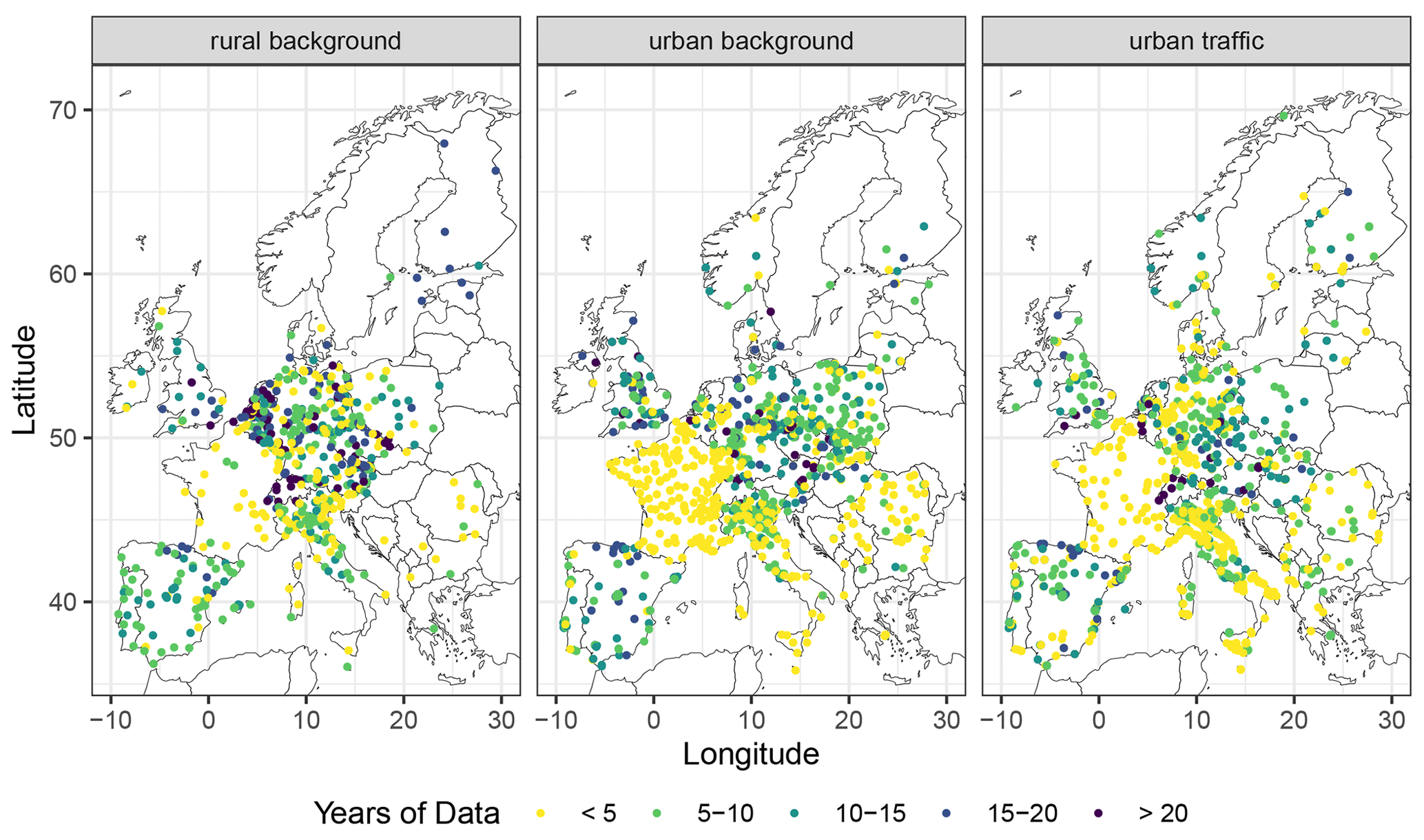
Figure 1Air quality monitoring stations from which NOx data are available through the AirBase database, coloured depending on the number of years that the provided records span. The stations are classified based on their locations as rural background, urban background, or urban traffic sites.
For some countries longer data sets seem to be available but are not provided in the AirBase database. For example, Font et al. (2019) conducted a study on air pollution in London and Paris where they used 10 years of NOx data – also for Paris where only less than 5 years of data per station were available in the database. For Austria the number of stations for which data are provided through AirBase dropped drastically from 2012 to 2013 even though according to the Environment Agency Austria all stations are still monitoring air quality up to date. Similar issues and findings with regards to the data availability through the database were also described in other studies and for other pollutants. For ozone, like for NOx, it was found that there is an uneven spatial distribution of stations with certain record lengths and that there are generally fewer sites in northern and eastern European countries and more sites in central Europe and Great Britain (Chang et al., 2017; EEA, 2009). It was also noted for ozone that longer data sets do exist outside AirBase and are available through other sources for some countries (EEA, 2009). Hence, these issues do not only apply to NOx, and it would be desirable to include all existing time series of air pollutant measurements in Europe in one database to allow long-term analyses which are not geographically biased or restricted to certain regions.
3.2 Urban and roadside increments
3.2.1 Urban increments
The mean UB levels for the nine cities were calculated based on all available UB data. For the mean RB levels rural stations were selected based on their distance to the city and data ranges. Table 1 lists the lower and upper limits for selecting RB sites as well as any outliers that were excluded before calculating averages. The RB data around Amsterdam and Linz did not show any consistent levels in the vicinity of the cities. These two cities were therefore considered unsuitable for the calculation of a mean RB level and with that also unsuitable for the analysis of an urban increment (UI).
Table 1Distance ranges within which rural background (RB) stations were considered to show consistent ranges, the outliers that were removed, and the final number of selected sites. “–” denotes that no lower limit was set or no outliers were removed.
For the seven cities where a consistent rural background level was found, UIs were calculated. In the following, all increments as well as emissions (see Sect. 3.3) will be presented both in absolute values and as percentages relative to a baseline year which was defined for each city based on the available data. The absolute UIs are shown in Fig. S1 in the Supplement and ranged between 23.34±3.62 µg m−3 in 2017 in Prague and 107.7±48.8 µg m−3 in 1997 in London. The percentage changes relative to the respective baseline years are shown in Fig. 2. The smallest reduction from the first to the last year with data was observed in Prague, where the UI decreased by 44.6 % from 1994 to 2017. Declines between 45 and 49 % over 20-year periods were estimated for Berlin, Augsburg, Geneva, and Vienna. In London the UI decreased by 52.0 % from 1996 to 2017, and in Zurich it decreased by 57.9 % between 1992 and 2017.

Figure 2Urban increments (UIs) and total emissions of NOx for seven European cities, relative to their values from a baseline year which was defined individually for each city dependent on the data availability. The UIs are derived from rural and urban background monitoring stations; emissions are averaged for the urban areas based on the EMEP emissions grid.
The absolute levels of the UIs exhibited a great variability. Torras Ortiz and Friedrich (2013) stated that it can be expected to find such variability when analysing UIs across different European countries due to the heterogeneity with regards to meteorology, topography, and emission release conditions across Europe. Since most of the analysed cities are located in central Europe, the meteorological differences are expected to be negligible at the assessed timescales. The other two factors are assumed to be of great importance, especially in the cities with high UIs. The high levels in London can most likely be linked to high emissions, as London has by far the highest total emissions per square kilometre out of the analysed cities (see Sect. 3.3). The second-highest UI values were observed for Geneva. Here, high emissions are unlikely to be the key factor leading to the observed high concentrations. In Geneva, the topography plays a more important role. The city is located at around 400 m a.s.l. at the end of a valley which opens up to the north-east, where Lake Geneva is situated. The remaining sides are framed with mountains which are between 1000 and 1700 m a.s.l. Cities in valley locations like this are known to show higher concentrations of air pollutants because they are prone to the formation of stable inversions, especially in winter, leading to an accumulation of pollutants near the surface (Schultz et al., 2017).
The change over time of the UIs is characterised for all cities by a downward trend and reductions of around 50 % throughout the analysed periods. Some cities, e.g. Zurich, show a relatively consistent decrease over time, while for other cities a stronger decline followed by stabilising values was observed. The latter was the case in Vienna, where the UI started to stabilise around 2000, and in London, where the last 10 years showed no strong trend. Studies on the trends of NOx measurements from different station types in the UK and London have found similar patterns: they observed a period that was characterised by decreasing concentrations followed by a period of more stable values (Carslaw et al., 2011a, b). In those studies, the change to more stable concentrations was observed between 2002 and 2004, while in the study at hand the downward trend extends until 2008. This slight difference can be mainly attributed to the different lengths of the analysed records: the last years examined here were not yet included in the earlier studies.
The share of the pollution measured in a city that can be attributed to sources within the urban area was found to be similar for most analysed cities. It can be estimated using the ratio of the UI to the UB concentration, and this ratio was calculated for each city and year. Overall, the ratios ranged between 55.9 and 84.5 % with a mean of 72.2 %. The highest average ratios were found in London and Ausgburg: 77.5 %. In Berlin, Zurich, and Prague the average ratios were between 70 and 75 %, and in Geneva and Vienna they were around 65 %. The ratio is usually distinctively higher for NOx than it is for PM, where only around half of the pollution measured in a city also originates in the urban area (Lenschow et al., 2002). This is due to the more local characteristics and shorter lifetime of NOx (Liu et al., 2016). The differences in the transport characteristics of the pollutants can affect the accuracy of the estimated UIs. Studies on PM criticised the characterisation of urban areas simply by their administrative borders instead of their actual urban sprawl or the extent of their commuting zones because it could lead to an underestimation of the total urban impact (Thunis, 2018; Torras Ortiz and Friedrich, 2013). This underestimation was not found for NOx, suggesting that taking commuting zones into account is of greater importance for pollutants that are easily transported in the atmosphere. When analysing cities with a great urban sprawl, it is nevertheless of particular importance to assess the data ranges of all surrounding RB stations prior to estimating a mean level to ensure that the stations actually represent rural rather than suburban conditions. As a result of doing so, the chances for underestimating the UI are drastically reduced.
For Amsterdam and Linz no UI could be calculated because no consistent RB level was found. For Amsterdam this is likely to be caused by the high urbanisation of the Netherlands. The Netherlands is considered one the most urbanised countries in Europe (Nabielek et al., 2016) and is also among the European countries with the highest population densities (Barrientos, 2019). The urban areas of the country are characterised by many small-to-medium-sized towns with relatively short distances between them (Nabielek et al., 2016). Some of the RB monitoring sites around Amsterdam are therefore likely influenced by urban areas, resulting in the great variation of concentration ranges that was observed.
The surrounding of Linz is not characterised by a particularly high urbanisation. Here, the varying topography in Austria and the positioning of some stations close to local emission sources such as industrial sites were hypothesised as potential causes for the varying data ranges. A detailed examination of the locations of the RB stations revealed that within the first 125 km of Linz all sites with a median greater than 20 µg m−3 are located east of Linz along the Danube River. While the other stations are spread in all directions around the city and are far from the river, the sites with higher values are all within a maximum of 3 km from the river bank. The Danube is an important shipping route, and inland waterway vessels were observed to emit great amounts of NOx (Pillot et al., 2016). Most vessels which are in operation nowadays use diesel engines without any emissions control because they were registered and have been in service since before the first European guidelines on emission limits for inland waterway vessels were introduced (Pillot et al., 2016). The high concentrations observed at some of the RB sites around Linz are therefore most likely caused by emissions from vessels on the river and should therefore not be considered representative of rural conditions.
3.2.2 The impact of atmospheric transport
The impact that urban pollution has on rural background sites due to atmospheric transport was assessed for the seven cities with consistent RB concentrations by calculating two mean RB levels: one based on downwind days and one based on all other days. For five of the cities, the mean RB level based on the downwind days is higher than the mean based on all days (see Fig. 3). This indicates that NOx is likely to be transported by wind from the cities to the surrounding rural areas. However, excluding the respective days leads to RB concentrations that differ only marginally from the RB concentrations where all days were included. When looking at annual NOx concentrations, the influence of atmospheric transport from a city to the rural areas was therefore found negligible.
For Augsburg and Geneva the results are not as clear. In both cases the mean RB levels based on the downwind days are in some years higher and in others lower than the averages of all days. A potential explanation for the values found in Augsburg is that some RB stations might also be influenced by atmospheric transport from a different near-by city. Munich is only 60 km away from Augsburg, and some stations might measure higher values on days when the wind is not coming from Augsburg because they are then downwind of Munich. Around Geneva the atmospheric transport is likely to be impacted by the surrounding topography as the city is situated at the end of a valley with high mountains rising on three sides. One of the assumptions of the conducted analysis is that the wind direction observed in a city can be taken as fairly representative for a bigger area around the city. While this simplified approach seems to lead to meaningful results for most cities, a very mountainous rural area could lead to a violation of this assumption. Furthermore, there are only three RB stations around Geneva that were considered representative for the mean RB level, and the data of those three stations were found problematic also for other analyses due to their relatively large data ranges.
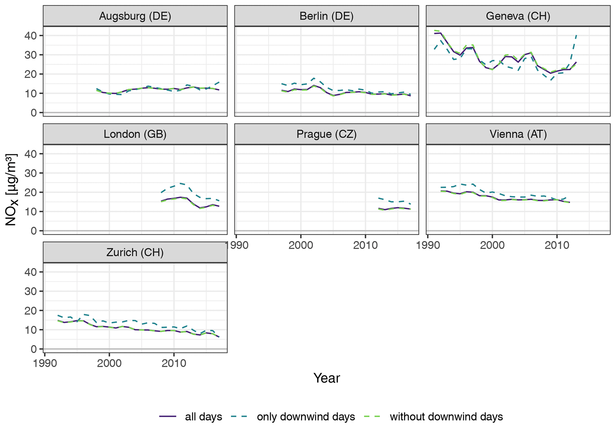
Figure 3The influence of atmospheric transport of NOx from cities to rural background (RB) stations. The depicted mean RB levels are based on three different subsets of daily data that were filtered by wind directions. “Downwind days” refers to all days when the wind blew within a 30∘ range from the city to a RB station.
3.2.3 Roadside increments
Roadside increments (RIs) were calculated for all nine selected cities, separately for each UT station. The time frames that were spanned by the increments differed greatly and ranged from 6 years in Amsterdam and Berlin to 27 years in Zurich and Prague. Similarly great variation was also found in the values themselves (Fig. S2). Both the highest and lowest RIs were estimated for two different stations in London. The overall highest value was 327.1 µg m−3 in 1991 at Cromwell Road in central London, and the overall lowest RI was −8.669 µg m−3 in 2003 at Kentish Way in the south-eastern London Borough of Bromley. Apart from London, RIs above 150 µg m−3 were only calculated for stations in Berlin. A few years with values above 100 µg m−3 were observed in Amsterdam, Augsburg, Prague, and Zurich, while the three remaining cities had lower RIs.
In Geneva, London, and Vienna negative RIs were calculated for some years at one station per city. A negative RI means that the concentration at the roadside location was lower than the urban background level in that year. In London the reason for this might be that the respective station is far from the city centre and that the calculated UB level is not representative for the conditions in that area. In a city of the size of London more accurate RIs might be obtained when estimating two different UB levels for the inner and outer city. In Vienna and Geneva, the observed negative RIs pose the question of whether the stations are placed properly at representative locations. It was noted that the distinction between background and traffic stations in Vienna is not as clear as for most other cities. Furthermore, different classifications of urban stations in Vienna according to the AirBase metadata and information from the Environment Agency Austria (Umweltbundesamt Österreich, 2017) were found. The latter classification was used.
Percentage changes relative to a common baseline year which was defined individually for each city dependent on the data availability were calculated for the RIs (Fig. 4). The strongest percentage change was observed at a station in Geneva where the RI decreased by 115.4 % from 1991 to 2014. The weakest reduction was found at a site in Amsterdam: the RI reduced by as little as 9.4 %. However, this was at one of the stations with a record of only 6 years, from 2012 to 2017. In most cities short periods or individual years with upward trends were observed, but in Linz both UT sites were found to have increasing RIs throughout the recorded period. They increased by 49.2 and 64.7 % from 1998 to 2012. Some UT sites in Amsterdam, Geneva, Linz, and Prague showed very strong year-to-year variations in the percentage changes due to relatively low RIs in the respective baseline years. The differences in the absolute values at those sites were small, at around 10 µg m−3, compared to the variations observed at other stations, e.g. in Berlin or London.
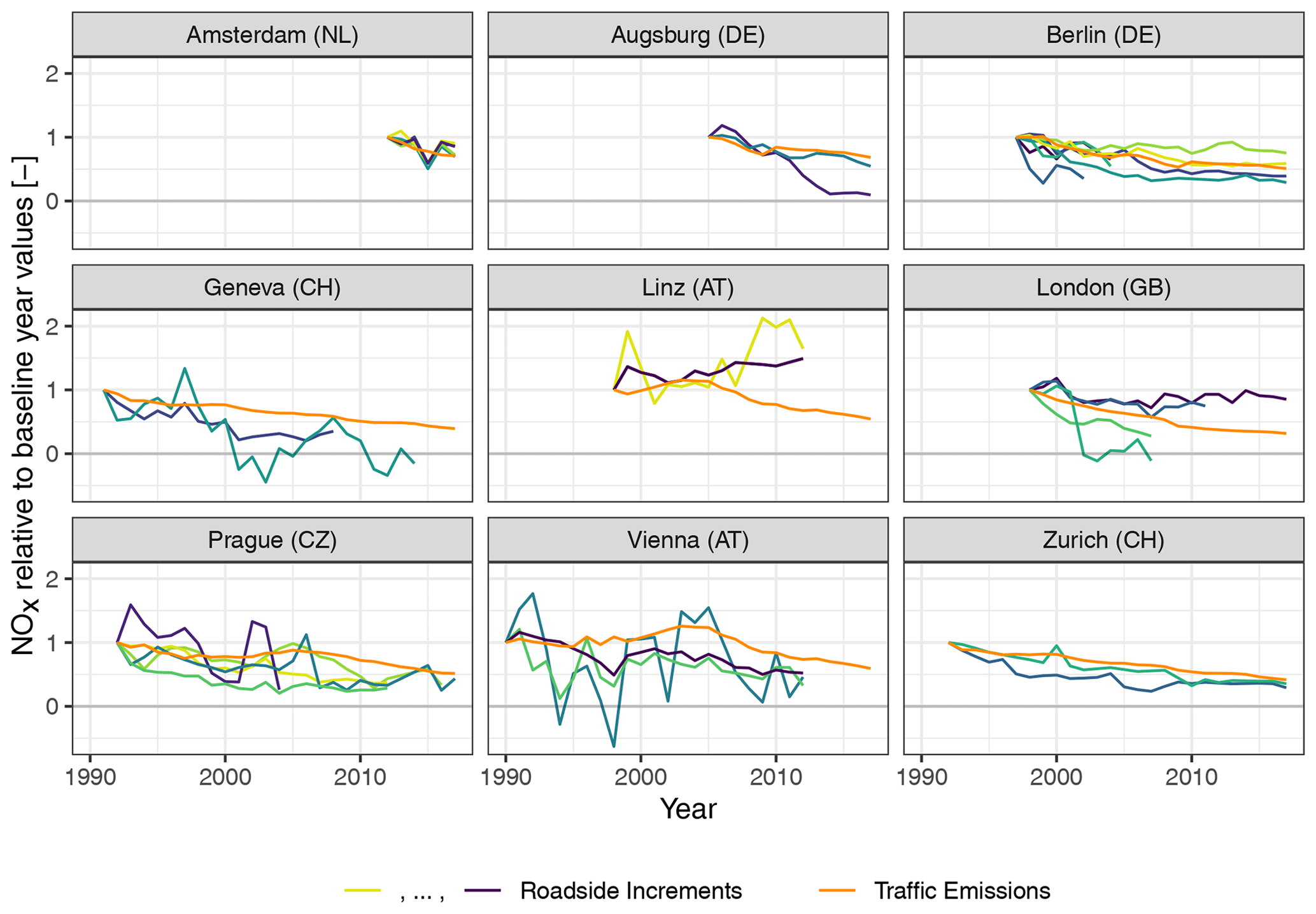
Figure 4Roadside increments (RIs) and traffic emissions of NOx for nine European cities, relative to their values from a baseline year which was defined individually for each city dependent on the data availability. The traffic emissions (orange lines) are averaged for the urban areas based on the EMEP emissions grid. All other lines depict individual RIs which are specific to a certain urban traffic monitoring station.
In most cities the direction of change agrees between the different RIs in the city. While the magnitude of change might differ, the sites from one city show either an upward or a downward trend. Only in some cities are there sites which were observed to have rather stable values, while other RIs from the same city continued to decrease. Great differences in the magnitudes of change were found, for example, in Augsburg and London. In Augsburg, one of the sites was at 54.6 % of the 2005 value in 2017, while the other station reduced down to 9.6 % in the same period. In London, at a station recording only 10 years of data the RI decreased to −11.0 % of its 1998 value, while another station was still at 85.3 % even after a 20-year period.
The reasons for differences in the magnitudes of change of several RIs in one city can be diverse. In London, three of the four sites providing data from 1998 to 2007 showed very similar declines over the 10-year period with regards to the absolute RIs: they all decreased by 75 to 85 µg m−3 (Fig. S2). Since they had measured very different levels in 1998, the percentage changes nevertheless showed the above-described discrepancy, which can be attributed to the very different characteristics of the locations of the UT sites. The station with high values and a smaller percentage reduction is situated in the inner city, while the other is located in the fringe area of London. For the two stations in Augsburg the discrepancy in change is present in the absolute and percentage values. The stronger decrease at one of the sites can be related to measures specific to that station: around 2010, the respective street was subject to extensive reconstructions which aimed at minimising the individual traffic and at expanding and strengthening the public transport (Stadtwerke Augsburg Verkehrs-GmbH swa, 2013). Most RIs are assumed to show a mix of the influence of the general trend typical for the respective city and the effects of local measures and local street characteristics.
Several studies have analysed the data of the monitoring sites in London over the last years. A large heterogeneity in the values and trends of UT sites has been observed (Font and Fuller, 2016). For the period 2004/2005 to 2009, Font and Fuller (2016) found that on average the RIs increased by around 1 % a−1, while Carslaw et al. (2011b) estimated downward trends in the NOx values from UT sites, and Beevers et al. (2012) found a decrease of around −2 % at streets in Outer London and a small increase or stable values at streets in Inner London. Even though the estimated trends vary, the different studies agree that the trends in the analysed years were rather small. This shows that in years with only slight changes or even stable values the selection and number of sites which are analysed and the way in which the results are aggregated can lead to different conclusions with regards to the overall trends. It also highlights that for RIs a separate assessment of the data of individual stations can lead to more and different insights than calculating an average RI.
3.3 Emission inventories
Total and traffic NOx emissions were averaged for each city based on the EMEP emission grid. Both showed overall declines from 1990 to 2017 in all cities even though in some cases periods of increases could be observed (Figs. S1 and S2). The total emissions were analysed for the same periods for which UIs were calculated; thus only seven of the nine cities and slightly different time frames for each city were assessed. The highest total emissions of 72.30 t km−2 were observed in 1996 in London, and the lowest in 2017 in Augsburg: 8.822 t km−2. The percentages relative to the baseline year values are depicted in Fig. 2. In Vienna, the emissions decreased by as little as 22.9 % from 1990 to 2012 and showed an increase between 1995 and 2003. In Geneva, Berlin, and Augsburg, emissions reduced between 35 and 45 % over periods of 23, 21, and 20 years, respectively. Reductions of around 50 % were observed in Prague from 1994 to 2017 and in Zurich from 1992 to 2017. The greatest decline was found in London: the emissions in 2017 were 67.0 % lower than in 1996.
The traffic emissions were assessed for all nine cities, but for different time periods depending on the baseline year of the RIs of each city. In Amsterdam the baseline year was set to 2012, and in the following 6 years the traffic emissions decreased by 29.1 %. A decrease of around 30 % was also found in Augsburg between 2005 and 2017. In this city, a slight increase of the emissions can be seen from 2009 to 2010. The same pattern is also present in the traffic emissions of Berlin, for the same years. Overall, the emissions decreased by around 50 % between 1997 and 2017 in Berlin. In Prague the emissions halved as well between 1992 and 2017, and in Geneva they decreased a bit more than half between 1991 and 2014. The other Swiss city, i.e. Zurich, showed a reduction by 58.3 % between 1992 and 2017. The two Austrian cities showed a similar pattern as was already observed for the total emissions in Vienna: the emissions increased until 2003 and then decreased again after 2005. In Vienna, the emissions were a quarter higher in 2003 than in 1990. Overall, they decreased by 26.3 %. In Linz, the reduction amounted to 32.3 % between 1998 and 2012. As was the case for the total emissions, the highest reduction in traffic emissions took place in London: a reduction by 68.3 % from 1998 to 2017.
Reductions in total emissions are linked, for example, to changes in the emissions from industrial sites in the cities or from the domestic heating sector (Senatsverwaltung für Stadtentwicklung und Umwelt, 2018). Reasons for the observed downward trends in traffic emissions are European emission standards and associated technology changes and end-of-pipe control measures (Crippa et al., 2016); updates of the vehicle fleets, which in turn can be accelerated for example by scrappage schemes or low-emissions zones (LEZs); the LEZs themselves; and local measures such as speed limits, road-specific vehicle restrictions, reconfigurations of road networks, or adaptive signalisation to reduce congestion (Bigazzi and Rouleau, 2017). It is difficult to attribute observed changes to specific measures, and the efficacy of the measures in bringing the levels down would have to be evaluated for each city individually and is not the focus of this study.
The trends in the emissions in Vienna and Linz did not show the continuous decline that was observed for the other cities. The peak between 2003 and 2005 was found to be also present in the national emission inventory and is linked to a large extent to an increase of the amount of fuel that was exported in the tanks of vehicles (Umweltbundesamt Österreich, 2016). It was estimated that roughly a quarter of the traffic emissions were actually caused in surrounding countries, due to the export of goods and relatively low fuel prices (Umweltbundesamt Österreich, 2016). This export of fuel is expected to be negligible in the cities, and adopting the upward trend of the national emissions to the trends in the cities might therefore lead to an overestimation of the actual change that was present in the traffic emissions of Vienna and Linz.
3.4 Comparison of increments and emissions
The increments of the NOx measurements were compared to the NOx emissions using the percentage changes of either one. RIs and traffic emissions were compared for all nine analysed cities, while UIs and total emissions were only compared for the seven cities where a consistent RB concentration could be estimated.
3.4.1 Total emissions and urban increments
For the majority of the seven cities the percentage changes observed in the UIs aligned fairly well with the changes of the total emissions, as can be seen in Fig. 2. Apart from Geneva and Vienna, the general trends of the NOx emissions seem to be reflected in the UIs. The UIs showed stronger annual variations than the emissions did, so the percentage change in the final years with data should be seen as momentary values, and the changes throughout the entire period should be considered to draw more meaningful conclusions. In Augsburg and Berlin emissions and UIs aligned well for the whole 20-year period, and also the percentage change values in 2017 differed only marginally between the two measures. In Prague the UI and the emissions were at around 55 and 50 %, respectively, of the baseline year values in 2017 and also generally showed similar declines throughout the analysed time frame. Despite the overall good agreement, there were more years when the emissions had reduced by a greater share than the UI had than the other way around. In London the same was observed but even more distinctly: only in 3 years were greater percentage reductions in the UI found than in the emissions. However, the discrepancy was relatively constant over time so that the change in the UI still seemed to follow the change in the emissions. In Zurich the opposite to what was seen in Prague and London was found: during most years the percentage change of the UI indicated greater reductions than that of the emissions. Nevertheless, the trends seemed to align well also in this city. In 2017, the UI had decreased by 57.9 %, and the total emissions by 49.8 %.
The two cities that showed relatively strong discrepancies between the temporal changes of the two measures were Geneva and Vienna. In the final years the differences amounted to 12.7 and 25.3 percentage points, respectively, but were even greater for many previous years. In Geneva, a good agreement was observed only for the first 2–3 years. Then, the UI showed a much stronger decline than the emissions for a few years, followed by a period when the changes were similar but at very different levels. In the last years, the emissions continued to decline at roughly the same rate as before, but the UI increased. In Vienna the discrepancy appeared even stronger. While the emissions started to increase at around 1995, the UI continued to decline, and when the emissions started to decrease in 2005 the UI stayed at a relatively constant level. In between, the percentage changes of the two measures differed by around 50 percentage points.
The more or less consistent discrepancies that were observed in London and Zurich can be related to the annual variability of the UIs. In both cities, the UIs showed strong changes between the first 2 years. In London for example, the UI increased by almost 20 µg m−3 from 1996 to 1997 and decreased again in the following year. Just as the value in the last year is a momentary value, so is the UI in the first year. If the data set of London had started 1 year later, the value of the baseline year would have been distinctively higher and the percentage reductions relative to that value therefore lower, resulting in a better agreement with the change of the emissions. Similarly, using 1993 as the baseline year instead of 1992 in Zurich would lead to a lower baseline value and also a better agreement with the percentage change of the total emissions. These examples show that the exact level of the relative reductions depends on the values in the baseline year and thus on the definition of that year. An agreement of how the percentage changes develop over time was therefore judged to be more important than an agreement in the exact percentage reductions for a specific year.
In Geneva and Vienna, a simple shift by defining a different baseline year could not resolve the discrepancies because these also extended to the change of the two measures over time. The peak in the emissions that was observed in Vienna is not reflected at all in the UI. In Sect. 3.3 it was discussed that the main cause of this peak was emissions from exported fuel. The discrepancy between the UI and the total emissions is therefore most likely based on differences between the emissions from used versus sold fuel in Austria. The discrepancy that was found for Geneva is likely related to inaccuracies in the UI rather than in the emissions. The UI of Geneva is – out of all seven UIs – the one that is based on the fewest monitoring sites, namely one UB station and three RB sites. Furthermore, the data measured at those stations differ in some ways to the data from comparable stations in and around other cities. However, the small number of stations makes it difficult to evaluate whether the measured concentrations can be considered accurate and representative for the respective location types.
Overall, the results support the assumption that a reduction in the total emissions should lead to a proportional reduction in the UI and that the latter can be attributed to the emission sources from the city, as was first stated by Lenschow et al. (2002). Apart from annual variations, long-term changes in total NOx emissions can give an idea about how the background concentrations in a city developed.
3.4.2 Traffic emissions and roadside increments
The percentage changes of the RIs span a very wide range, also in their relation to the traffic emissions. For some UT sites the estimated RIs showed a stronger decline than the emissions, while others reduced less. Similarly, there is a lot of variation between the cities, as can be seen in Fig. 4. In some cities the RIs and the emissions seem to align well, e.g. in Zurich; in others there is a great discrepancy, e.g. in Linz; and in yet others the different UT stations within a city show different signals and agree to varying levels with the emissions, e.g. in Berlin and London.
In Amsterdam, all five RIs showed a similar pattern of annual variations throughout the 6 years with data, with a distinct dip in 2015. The emissions declined relatively consistently during the same period. In 2017, two RIs had declined by 30 % relative to the 2012 values – just as the emissions had. The other three sites decreased by only 10 to 15 %. Overall, the reductions in the RIs and the traffic emissions seem to align for Amsterdam, but with just 6 years of data it is hard to judge. A very interesting feature in the traffic emissions of the city was observed from 2009 to 2010, when the values dropped by around 10 t km−2. Unfortunately, not enough RIs could be calculated for that time to evaluate whether the drop in the emissions was reflected in the measured concentrations.
In Augsburg, the two RIs were found to have changed very differently after 2010: one decreased by around 55 % from 2005 to 2017, while the other reduced by over 90 %. The emissions showed a reduction of around 32 %. The trends in the percentage changes appeared to agree well between the emissions and the first RI even though the values in the final year differed. The other RI showed a much stronger decline than the emissions, which – as was discussed before – could be related to reconstructions of the street network near the respective UT site. The RI is therefore considered to represent rather local changes in ambient concentrations, and it is not surprising that these do not align with the changes of the average traffic emissions of the city.
Berlin had a wide range of percentage changes in the RIs: the values were at 29.0 to 74.5 % of their 1997 levels in 2017. Over the same period, the traffic emissions reduced to 51.0 % of their 1997 level. Three of the four long-term UT sites showed similar reductions until around 2005, subsequently diverging to different levels. Until 2005 the percentage reduction of the emissions was also in line with that of the three UT sites. The RI of the fourth station diverged earlier and ended at a percentage level well below that of the emissions. The stronger decline observed at that station is linked to a set of local measures: in 2000 a speed limit of 30 km h−1 was introduced and an extension of an urban motorway parallel to the street was completed (Senatsverwaltung für Umwelt, Verkehr und Klimaschutz, 2019), and in 2005 heavy goods vehicles weighing more than 3.5 t were banned from driving through the street with the exception of originating or terminating traffic (Senatsverwaltung für Stadtentwicklung und Umwelt, 2013).
The two RIs that could be calculated for Geneva showed similar trends and patterns in their absolute values but differed by around 50 µg m−3 in the baseline year, 1991. Due to their different starting levels their percentage changes also differed substantially in some years. Compared to the traffic emissions, both showed stronger percentage reductions. The site with higher RI values only provided data until 2008. By that time the RI had decreased by 65 % relative to 1991, while the emissions had reduced by only 41 %. In that year, the other RI showed almost the exact same percentage reduction as the emissions: 44 %. However, this was only momentary because the RI peaked in that year. After 2008 the RI declined – even to negative values – and in 2014 it was at −15 % of its 1991 value. The emissions were at 47 % of their baseline level in that year. Overall, the RIs showed slightly steeper declines than the emissions especially in the first 10 years and seemed to stabilise around 2005, while the emissions showed a continuous decline.
In Linz, a strong discrepancy between the RIs and the emissions was found, especially in the second half of the analysed period. From 1998 to 2003 or 2005 the two RIs and the emissions showed similar increases. By 2003, the emissions had increased to 116 % of their baseline value, and the RIs to 105 and 115 %. In the following years they developed quite differently: the emissions started declining and in 2012 were at 68 % of the 1998 level. The RIs on the other hand kept increasing to 165 and 149 % of their baseline levels. The two UT sites are located in very different areas of the city, so that the upward trends are unlikely to be caused by a local measure but are rather linked to the general development of the city. Linz developed from a “steel city” to an important service and cultural centre in Upper Austria and a vibrating, lively, and growing city with a high number of daily commuters from surrounding municipalities (Amt der Oberösterreichischen Landesregierung, 2018). Furthermore, Linz is considered a trans-European transport nodal point (Amt der Oberösterreichischen Landesregierung, 2018). From 2001 to 2011, the total number of journeys in the city increased by almost 18 % (Magistrat der Landeshauptstadt Linz, 2012). This strong increase is most likely what drove the observed increase in the RIs. The traffic emissions of Linz do not show a comparable upward trend as the gridding of the national EI does not account for such local changes.
London is one of the cities where some RIs decreased more and others less than the emissions did. The two sites with stronger percentage changes only provide data until 2007, and in that year the respective RIs are at −11 and 28 % of their 1998 levels. The emissions decreased to 58 % of their baseline level. The other two RIs are at 57 and 72 % of their 1998 values in 2007 and show relatively stable values or slight increases in the years afterwards. The only RI that could still be calculated for 2017 was at 85 % of the baseline value, as opposed to the emissions, which were at 32 %. In Sect. 3.2.3, it was discussed that one reason for the strong differences in the percentage changes of the four RIs is the different characteristics of the stations' locations. The station where the RI showed negative values is situated in one of London's outskirts, while the station with the weakest decrease is in the inner city. London is the biggest of the analysed cities and therefore shows a lot of variation within the city. Nevertheless, the emissions were averaged over the entire urban area to retain consistency with the other cities. To compare RIs with emissions that are more representative of the area where a respective UT site is located, it might be useful to split all data into Inner and Greater London.
For Prague, many RIs could be calculated, and most of them showed similar trends. In the first 5 years after 1992 the decrease of the majority of the RIs agreed with the trend of the emissions. In the following years the RIs generally decreased further – apart from annual fluctuations – while the emissions increased slightly until 2005 and then decreased again. In 2012, four UT sites had provided data, and the corresponding RIs had all reduced by around 60 to 70 % relative to 1992. The emissions had only reduced by 34 % in the same period. In 2017, the only remaining RI had decreased by 56 %, and the emissions by 48 %, so that integrated over the entire period the percentage changes were almost identical. However, the way the RIs and the emissions changed over time did not align very well, and generally most RIs showed stronger reductions for most of the time than the traffic emissions did.
The traffic emissions in Vienna showed a peak around 2004, just as was observed for the traffic emissions of Linz and the total emissions of Vienna. The three RIs did not follow that trend. One RI also showed high percentage change values from 2003 to 2005, but this RI had rather low and partly even negative absolute values, so that the percentage values fluctuated quite strongly. The other two RIs increased from 1998 to 2001 but then started decreasing while the emissions were still increasing. As was mentioned before, the emission peak would probably not be present if the EI excluded emissions from exported fuel, and so the RIs were not expected to reflect that trend. In 2003, the emissions were at 126 % of their 1990 level, and the RIs at 66, 86, and 149 %. In the last year with data, i.e. 2012, the emissions were at 74 % of the baseline value, while the RIs had decreased to 33 to 52 % of their values from 1990.
Zurich shows a relatively good agreement between the percentage changes of the traffic emissions and one of the RIs even though the latter stabilised in recent years while the emissions continuously declined. The other RI showed a stronger decrease until around 1998 and then started to level off or slightly decrease. From 2010 onwards the percentage changes observed in both RIs were very similar to each other and showed no distinct trend. By 2017, both had reduced by 65 to 70 % of their 1992 levels. During the same period the traffic emissions decreased by 58 %. The stronger percentage change of one of the RIs in the first years is to a large extent due to the lower absolute value in the baseline year. The stabilisation of the RIs after 2010 while the emissions kept declining could indicate that the amount of NOx that was actually emitted in the city did not decrease as suggested by the EI. Similar findings were described in other studies and related to the discrepancies between NOx emission factors and real-world emissions from diesel vehicles as will be discussed in more detail further down in this section.
Overall, the RIs did not align as well with the emissions as the UIs did. They are more locally influenced, which is why even RIs from the same city can show very different values and trends. RIs can be impacted by the characteristics of the street, like its width or its orientation relative to the main wind direction, as well as by local measures, like restrictions for certain vehicles, the introduction of speed limits, or a reconfiguration of the road network. Differences between RIs in the inner city as opposed to the outskirts of a big city were observed in London. All these are factors which impact the ambient NOx concentrations very locally and which are not expected to affect the average traffic emissions of a city. Other measures, like the introduction of a LEZ, could potentially influence the concentrations at all UT sites within the zone, and their effects should also be seen in the average emissions due to the larger areal scope of the measures. All policies that affect the entire city or at least large parts of it should – if they are effective – lead to reductions in the average traffic emissions that are reflected in the RIs. Rather local measures on the other hand are one of the reasons for the discrepancies that were observed in the trends of RIs and traffic emissions.
Another reason for a poor agreement between the changes of emissions and RIs is that the EIs did not necessarily represent the actual changes of traffic emissions in the city. Rather, the EIs represent the emission changes observed at a national scale, and only the absolute levels were downscaled according to local characteristics. Especially the case of Linz demonstrated how this can lead to distinct discrepancies between the changes of emissions and RIs. In a study on London, the London Atmospheric Emission Inventory (LAEI) and the National Atmospheric Emission Inventory (NAEI) of the United Kingdom were compared to measurements of ambient NOx concentrations (Lee et al., 2015). The study found “a much closer agreement” of the measurements with the LAEI than with the NAEI and related that to the more accurate representation of traffic in London and thus more accurate traffic emissions. Another study on London also stated that using national EIs in analyses that focus on local scales can increase the degree of uncertainty in the results (Beevers et al., 2012). For studies that focus on cities, more accurate and meaningful results could be obtained if local instead of national EIs were used. However, it was noted that it can be difficult to obtain such local EIs and that they are sometimes very scarce in the number of years for which data are available.
Many studies, especially in London and the UK, have found similar disparities between the trends of NOx and NO2 emissions and ambient concentrations (e.g. Beevers et al., 2009, 2012; Carslaw et al., 2011b; Font and Fuller, 2016; Lee et al., 2015). Even when different EIs that were based on various sets of emission factors or activity data were analysed, none of them were found to agree sufficiently well with the changes in the concentration measurements (Beevers et al., 2012; Lee et al., 2015). Some compared better,while others showed very poor agreement, but overall it was noted that the estimated trends in the emissions were “too optimistic” compared with the observed measurement trends (Beevers et al., 2012). Using remote sensing data led to the conclusion that emission factors that were used in those EIs were generally underestimating the real emissions, particularly from some vehicle classes (Carslaw et al., 2011a, b). The assessments indicated that the theoretical reduction of NOx emissions from diesel vehicles as it was required by stricter emission standards did not actually take place and that some newer passenger cars still emitted at the same level as the previous generation cars had (Carslaw et al., 2011a, b). This disparity between emission factors and real-world emissions was identified as the main cause for the stronger reductions in the emissions than in the observed concentrations (Carslaw et al., 2011a). In the study at hand, it is difficult to evaluate to what extent the observed discrepancies are related to false emission factors which do not reflect real-world emissions because of the previously discussed factors that might also play a role.
Another potential reason for discrepancies between the trends of emissions and the trends of ambient concentrations is the impact of climate variability (e.g. Beevers et al., 2009; Yao and Zhang, 2020). Here, this influence is negligible due to the incremental approach: urban background concentrations and roadside concentrations within one city are affected by the same climatic variations, especially when looking at annual scales, and calculating the difference between these concentrations therefore minimises any climatic trend in the data.
The observed disparities between the trends in the RIs and the traffic emissions are in most cases linked to a combination of all of the discussed factors, like local differences within a city, a poor representation of changes specific to the city by the EI, and inaccurate emission factors for some vehicle classes. The importance of each factor and how strongly they affect the individual RIs can vary from city to city and probably even from UT site to UT site. Nevertheless, the fact that changes in RIs are in most cases not directly proportional to changes in estimated traffic emissions has some important implications. If EIs are used for future projections of ambient concentrations of NOx in cities, the large uncertainties associated with that have to be taken into account. Trying to forecast how the air quality will improve in cities by using the trends of national EIs could lead to massive biases as was shown particularly by the example of Linz and as was also stated by Beevers et al. (2012). Similarly, assuming the emissions will reduce as indicated by the emission factors has proven to lead to a potential overestimation of the trends in the ambient concentrations (Beevers et al., 2009). The high uncertainty associated with emission factors should not be ignored when drawing conclusions about future concentrations of air pollutants based on EIs. Especially when trying to evaluate future health impacts or compliance with limit values at the street level, the general uncertainties as well as the local differences within a city need to be considered to ensure an efficient management of air pollution that is caused by traffic.
Trends in ambient concentrations and emission inventories of NOx were compared using the incremental approach. Urban and roadside increments were calculated for nine European cities which were selected based on the availability of NOx measurements through the AirBase database. These cities are Amsterdam, Augsburg, Berlin, Geneva, Linz, London, Prague, Vienna, and Zurich. Furthermore, the potential impact that urban pollution might have through atmospheric transport on rural background (RB) concentrations was assessed to evaluate the accuracy of urban increments (UIs) of NOx.
The analysis of the availability of NOx observations through the AirBase database revealed some distinct regional differences. Both the number of stations and the lengths of the provided data records were higher in central Europe and Great Britain compared to any other part of Europe. Accordingly, the analysis of European cities was limited to this region. It was further restricted to very few cities due to short records, data gaps, and temporally non-overlapping records of urban background (UB) and urban traffic (UT) sites. Particularly extensive data sets were available for Berlin and Prague, where high numbers of UB and UT sites provided data records for 20 or more years, and records of the same lengths could also be compiled from the surrounding RB stations. While more data seem to be available outside the AirBase database, the data provided there set serious limitations to the analysis of long-term trends in increments in pan-European studies.
Assessing the impact of urban pollution on rural concentrations showed that atmospheric transport from cities to rural sites is negligible when annual averages of NOx are considered. On the days when the wind came from a city towards a RB station the measured concentrations were usually higher, but excluding those values had almost no effect on the annual averages. This could be different if UIs were analysed on shorter timescales, e.g. daily, or for other pollutants, e.g. PM.
Analysing the UIs showed that the assumption of finding consistent UB and RB levels in and around an urban area is true for most cities. However, for two of the nine cities the RB stations in the surrounding area did not show consistent concentrations, so that those cities were considered unsuitable for calculating UIs. The reasons for that were a very densely populated country with few actually rural areas around Amsterdam and a clear impact of inland waterway vessels on the Danube River at some of the RB sites around Linz. For the remaining seven cities consistent concentration levels were found, and UIs were calculated and compared to total emissions. The percentage changes of the two measures generally aligned well, as was expected. Only for two cities, i.e. Vienna and Geneva, did the changes of emissions and UIs differ. The discrepancies could be attributed to the emission inventory in one case and to probable inaccuracies in the UI in the other case. Over the analysed time frames from 20 to 25 years the UIs and the emissions showed overall downward trends in all cities. The UIs decreased by 45 to 60 %, and the total emissions by 23 to 67 %, but not continuously in some cities. The share of the NOx concentrations measured in a city that originates in the urban area was estimated using the ratio of the UI to the UB level. For the different cities, the ratio ranged between 55 and 85 % with a mean around 70 %, which shows that a great part of the NOx air pollution in a city is caused by activities within the city itself. Measures for reducing NOx concentrations should therefore strongly focus on the emission sources within urban areas.
The analysis of roadside increments (RIs) revealed a great variability within and across cities both in absolute levels and in trends. Most RIs showed general downward trends, but in some cities increasing values were found. Furthermore, some RIs decreased to negative values, raising questions about the adequacy of the locations and type classifications of the respective UB and UT sites. The traffic emissions showed overall downward trends in all cities with increasing values for a few years in some urban areas. The relation of changes in RIs to changes in traffic emissions was found to vary strongly, again within as well as across cities. In some cases, the discrepancies between the trends in traffic emissions and RIs might be related to inaccurate emission factors in the emissions inventories (EIs). However, there are also other important factors playing a role. City averages of traffic emissions do not accurately represent the emissions at the street level, and, furthermore, RIs are impacted by very site-specific factors such as speed limits or changes in the near-by road network. Considering the trend in a RI representative for how NOx concentrations generally changed at the street level of the respective city should therefore be viewed critically. Nevertheless, RIs provide valuable insight into how certain methods for emission reductions impact the ambient NOx concentrations at streets.
With regards to the mitigation of exceedances of limit values it became very clear that a strong focus should be the reduction of NOx emissions from sources which emit within urban areas as these are responsible for roughly three-quarters of the NOx air pollution in cities. Only a minor part stems from sources in the surrounding areas. Furthermore, the study revealed distinct differences between EIs and RIs which should be accounted for when using EIs to evaluate future health impacts or compliance with limit values at the street level. Only by considering these strong local differences within cities can an efficient management of air pollution in urban areas be ensured.
A more accurate comparison of trends in emissions with trends in increments could be achieved if EIs were available that are more representative of the true urban emissions. Ideally, the EIs should not include emissions from exported fuel, and the temporal changes should be downscaled or adopted properly to local changes in emission sources. While these more local EIs with a decent temporal resolution can be accessed for some cities, the current availability is limited for pan-European studies. Similarly, also the provisioning of NOx observations limits an analysis to certain European regions. It would have been interesting to include cities in other parts of Europe to assess how differences in meteorological conditions, e.g. between north and south, or differences in how traffic volumes and vehicle ages changed, e.g. between east and west, would have impacted the increments and their trends, but the available data did not allow for this. To be able to explore these aspects in future studies, access through the AirBase database to long-term records measured in cities across the whole of Europe would be very valuable. While the incremental approach was evaluated as a useful tool – particularly for NOx, where potentially confounding factors were found to be negligible – its application to long-term pan-European studies is currently restricted due to data availability.
The underlying code is available at https://doi.org/10.5281/zenodo.4604890 (Macdonald, 2021).
The data that were used are from third parties and freely accessible through their data repositories. Ambient concentration measurements can be found in the Airbase repository from the European Environment Agency (https://discomap.eea.europa.eu/map/fme/AirQualityExport.htm; EEA, 2019b), and gridded emissions data are available from the repository of the EMEP Centre of Emission Inventories and Projections (https://www.ceip.at/the-emep-grid/gridded-emissions/nox; EMEP CEIP, 2020).
The supplement related to this article is available online at: https://doi.org/10.5194/acp-21-4007-2021-supplement.
TB conceived the study and guided the data analysis. NO prepared the raw AirBase data set. EM performed the analysis and wrote the paper with contributions from each author.
The authors declare that they have no conflict of interest.
This work was hosted by IASS Potsdam, with financial support provided by the Federal Ministry of Education and Research of Germany (BMBF) and the Ministry for Science, Research and Culture of the State of Brandenburg (MWFK). Ambient concentration measurements were obtained through the AirBase (EEA) repository. Gridded emissions data were obtained from the EMEP (CEIP). Wind data were provided by CHMU, DWD, MeteoSchweiz, Met Office, and ZAMG. Elena Macdonald acknowledges the valuable discussions with and comments by Erika von Schneidemesser.
This research has been supported by the Bundesministerium für Bildung und Forschung (grant no. 01US1701).
This paper was edited by Leiming Zhang and reviewed by two anonymous referees.
Amt der Oberösterreichischen Landesregierung: Mobilitätsleitbild für die Region Linz, available at: https://www.linz.at/images/mobilitaetsleitbild_kumm_steig_um.pdf (last access: 15 July 2020), 2018. a, b
Barrientos, M.: Population density, Europe, available at: https://www.indexmundi.com/map/?v=21000&r=eu&l=en (last access: 14 April 2020), 2019. a
Beevers, S. D., Carslaw, D. C., Westmoreland, E., and Mittal, H.: Air pollution and emissions trends in London, King's College London and the Institute for Transport Studies, available at: https://www.researchgate.net/publication/242635799_Air_pollution_and_emissions_trends_in_London (last access: 26 July 2020) 2009. a, b, c, d, e, f, g, h, i
Beevers, S. D., Westmoreland, E., de Jong, M. C., Williams, M. L., and Carslaw, D. C.: Trends in NOx and NO2 emissions from road traffic in Great Britain, Atmos. Environ., 54, 107–116, https://doi.org/10.1016/j.atmosenv.2012.02.028, 2012. a, b, c, d, e, f, g
Bigazzi, A. Y. and Rouleau, M.: Can traffic management strategies improve urban air quality? A review of the evidence, J. Transp. Health, 7, 111–124, https://doi.org/10.1016/j.jth.2017.08.001, 2017. a
Carslaw, D. C. and Beevers, S. D.: Estimations of road vehicle primary NO2 exhaust emission fractions using monitoring data in London, Atmos. Environ., 39, 167–177, https://doi.org/10.1016/j.atmosenv.2004.08.053, 2005. a, b
Carslaw, D. C., Beevers, S. D., Tate, J. E., Westmoreland, E. J., and Williams, M. L.: Recent evidence concerning higher NOx emissions from passenger cars and light duty vehicles, Atmos. Environ., 45, 7053–7063, https://doi.org/10.1016/j.atmosenv.2011.09.063, 2011a. a, b, c, d, e, f, g, h
Carslaw, D. C., Beevers, S. D., Westmoreland, E., Williams, M., Tate, J., Murrells, T., Stedman, J., Li, Y., Grice, A., Kent, A., and Tsagatakis, I.: Trends in NOx and NO2 emissions and ambient measurements in the UK, available at: https://uk-air.defra.gov.uk/assets/documents/reports/cat05/1108251149_110718_AQ0724_Final_report.pdf (last access: 25 June 2020), 2011b. a, b, c, d, e
Chang, K.-L., Petropavlovskikh, I., Copper, O. R., Schultz, M. G., and Wang, T.: Regional trend analysis of surface ozone observations from monitoring networks in eastern North America, Europe and East Asia, Elem. Sci. Anth., 5, 50, https://doi.org/10.1525/elementa.243, 2017. a
Council of the European Union: Council Directive 85/203/EEC of 7 March 1985 on air quality standards for nitrogen dioxide, CELEX: 31985L0203, available at: https://eur-lex.europa.eu/legal-content/EN/TXT/?uri=CELEX:31985L0203 (last access: 12 March 2021), 1985. a
Crippa, M., Janssens-Maenhout, G., Dentener, F., Guizzardi, D., Sindelarova, K., Muntean, M., Van Dingenen, R., and Granier, C.: Forty years of improvements in European air quality: regional policy-industry interactions with global impacts, Atmos. Chem. Phys., 16, 3825–3841, https://doi.org/10.5194/acp-16-3825-2016, 2016. a
EEA (European Environment Agency): Assessment of ground-level ozone in EEA member countries, with a focus on long-term trends, Technical Report 7, EEA, Copenhagen, Denmark, 52 pp., 2009. a, b, c
EEA (European Environment Agency): Air quality in Europe – 2019 Report, Technical Report 10, EEA, available at: http://www.eea.europa.eu/publications/air-quality-in-europe-2019 (last access: 16 April 2020), 2019a. a, b
EEA (European Environment Agency): Download of air quality data – E1a and E2a data, Copenhagen, Denmark, available at: https://discomap.eea.europa.eu/map/fme/AirQualityExport.htm (last access: 15 March 2021), 2019b. a
Elser, M., Bozzetti, C., El-Haddad, I., Maasikmets, M., Teinemaa, E., Richter, R., Wolf, R., Slowik, J. G., Baltensperger, U., and Prévôt, A. S. H.: Urban increments of gaseous and aerosol pollutants and their sources using mobile aerosol mass spectrometry measurements, Atmos. Chem. Phys., 16, 7117–7134, https://doi.org/10.5194/acp-16-7117-2016, 2016. a, b
EMEP CEIP (Centre on Emission Inventories and Projections): Gridded NOx data, Vienna, Austria, available at: https://www.ceip.at/the-emep-grid/gridded-emissions/nox (last access: 15 March 2021), 2020. a
European Parliament and Council of the European Union: Directive 2008/50/EC of the European Parliament and of the Council of 21 May 2008 on ambient air quality and cleaner air for Europe, CELEX: 32008L0050, available at: https://eur-lex.europa.eu/legal-content/EN/TXT/?qid=1615566576777&uri=CELEX:32008L0050 (last accessed: 12 March 2021) 2008. a
Faustini, A., Rapp, R., and Forastiere, F.: Nitrogen dioxide and mortality: Review and meta-analysis of long-term studies, Eur. Respir. J., 44, 744–753, https://doi.org/10.1183/09031936.00114713, 2014. a
Font, A. and Fuller, G. W.: Did policies to abate atmospheric emissions from traffic have a positive effect in London?, Environ. Pollut., 218, 463–474, https://doi.org/10.1016/j.envpol.2016.07.026, 2016. a, b, c, d, e
Font, A., Guiseppin, L., Blangiardo, M., Ghersi, V., and Fuller, G. W.: A tale of two cities: is air pollution improving in Paris and London?, Environ. Pollut., 249, 1–12, https://doi.org/10.1016/j.envpol.2019.01.040, 2019. a, b, c, d, e
Grange, S. K.: Technical note: Averaging wind speeds and directions, https://doi.org/10.13140/RG.2.1.3349.2006, 2014. a
Guerreiro, C. B., Foltescu, V., and de Leeuw, F.: Air quality status and trends in Europe, Atmos. Environ., 98, 376–384, https://doi.org/10.1016/j.atmosenv.2014.09.017, 2014. a, b
Lang, P. E., Carslaw, D. C., and Moller, S. J.: A trend analysis approach for air quality network data, Atmos. Environ., 2, 100030, https://doi.org/10.1016/j.aeaoa.2019.100030, 2019. a, b
Lee, J. D., Helfter, C., Purvis, R. M., Beevers, S. D., Carslaw, D. C., Lewis, A. C., Møller, S. J., Tremper, A., Vaughan, A., and Nemitz, E. G.: Measurement of NOx fluxes from a tall tower in central London, UK and comparison with emissions inventories, Environ. Sci. Technol., 49, 1025–1034, https://doi.org/10.1021/es5049072, 2015. a, b, c, d, e
Lenschow, P., Abraham, H.-J., Kutzner, K., Lutz, M., Preu, J.-D., and Reichenbacher, W.: Some ideas about the sources of PM10, Atmos. Environ., 35, 23–33, https://doi.org/10.1016/s1352-2310(01)00122-4, 2002. a, b, c, d, e
Liu, F., Beirle, S., Zhang, Q., Dörner, S., He, K., and Wagner, T.: NOx lifetimes and emissions of cities and power plants in polluted background estimated by satellite observations, Atmos. Chem. Phys., 16, 5283–5298, https://doi.org/10.5194/acp-16-5283-2016, 2016. a
Macdonald, E.: Code for A Comparison of Long-term Trends in Observations and Emission Inventories of NOx, Zenodo, https://doi.org/10.5281/zenodo.4604890, 2021. a
Magistrat der Landeshauptstadt Linz: Gesamtes Verkehrsaufkommen in Linz, available at: http://www.linz.at/zahlen/050_Infrastruktur/050_Verkehr/ (last access: 15 July 2020), 2012. a
Mills, I. C., Atkinson, R. W., Kang, S., Walton, H., and Anderson, H. R.: Quantitative systematic review of the associations between short-term exposure to nitrogen dioxide and mortality and hospital admissions, BMJ Open, 5, 1–8, https://doi.org/10.1136/bmjopen-2014-006946, 2015. a
Nabielek, K., Hamers, D., and Evers, D.: Cities in the Netherlands, PBL Netherlands Environment Assessment Agency, The Hague, the Netherlands, 31 pp., 2016. a, b
Petetin, H., Beekmann, M., Sciare, J., Bressi, M., Rosso, A., Sanchez, O., and Ghersi, V.: A novel model evaluation approach focusing on local and advected contributions to urban PM2.5 levels – application to Paris, France, Geosci. Model Dev., 7, 1483–1505, https://doi.org/10.5194/gmd-7-1483-2014, 2014. a
Pey, J., Querol, X., and Alastuey, A.: Discriminating the regional and urban contributions in the North-Western Mediterranean: PM levels and composition, Atmos. Environ., 44, 1587–1596, https://doi.org/10.1016/j.atmosenv.2010.02.005, 2010. a, b, c
Pillot, D., Guiot, B., Cottier, P. L., Perret, P., and Tassel, P.: Exhaust emissions from in-service inland waterways vessels, J. Earth Sci. Geotech. Eng., 6, 205–225, 2016. a, b
QGIS Development Team: QGIS Geographic Information System, QGIS Association, available at: http://www.qgis.org (last access: 2 July 2020), 2019. a
R Core Team: R: A Language and Environment for Statistical Computing, R Foundation for Statistical Computing, Vienna, Austria, available at: https://www.R-project.org/, last access: 20 July 2020. a
Richter, A.: Nitrogen oxides in the troposphere – What have we learned from satellite measurements?, EPJ Web of Conferences, 1, 149–156, https://doi.org/10.1140/epjconf/e2009-00916-9, 2009. a
RStudio Team: RStudio: Integrated Development Environment for R, RStudio, Boston, USA, available at: http://www.rstudio.com/ (last access: 20 July 2020), 2019. a
Schultz, M. G., Klemp, D., and Wahner, A.: Luftqualität, in: Klimawandel in Deutschland, edited by: Brasseur, G., Jacob, D., and Schuck-Zöller, S., Springer Spektrum, Berlin and Heidelberg, Germany, 127–136, https://doi.org/10.1007/978-3-662-50397-3_13, 2017. a
Senatsverwaltung für Stadtentwicklung und Umwelt: Luftreinhalteplan 2011 bis 2017 für Berlin, available at: http://www.stadtentwicklung.berlin.de/umwelt/luftqualitaet/de/luftreinhalteplan/download/Luftreinhalteplan_Berlin_2011.pdf (last access: 17 February 2020), 2013. a
Senatsverwaltung für Stadtentwicklung und Umwelt: Langjährige Entwicklung der Luftqualität (Ausgabe 2018), available at: https://www.stadtentwicklung.berlin.de/umwelt/umweltatlas/e_text/k312.pdf (last access: 10 April 2020), 2018. a
Senatsverwaltung für Umwelt, Verkehr und Klimaschutz: Luftreinhalteplan für Berlin – 2. Fortschreibung, available at: https://www.berlin.de/senuvk/umwelt/luft/luftreinhaltung/luftreinhalteplan_2025/download/Luftreinhalteplan.pdf (last access: 15 May 2020), 2019. a
Stadtwerke Augsburg Verkehrs-GmbH swa: Der neue Kö, available at: https://www.projekt-augsburg-city.de/m-i-c-r-o-s-i-t-e-s/der-neue-koe/der-neue-koe/ (last access: 23 April 2020), 2013. a
Thunis, P.: On the validity of the incremental approach to estimate the impact of cities on air quality, Atmos. Environ., 173, 210–222, https://doi.org/10.1016/j.atmosenv.2017.11.012, 2018. a, b, c, d, e, f
Torras Ortiz, S. and Friedrich, R.: A modelling approach for estimating background pollutant concentrations in urban areas, Atmos. Pollut. Res., 4, 147–156, https://doi.org/10.5094/APR.2013.015, 2013. a, b, c, d, e
Umweltbundesamt Österreich: Klimaschutzbericht 2016, available at: https://www.umweltbundesamt.at/fileadmin/site/publikationen/REP0582.pdf (last access: 12 March 2021), 2016. a, b
Umweltbundesamt Österreich: Luftgütemessstellen in Österreich, available at: https://www.umweltbundesamt.at/fileadmin/site/publikationen/REP0607.pdf (last access: 20 April 2020), 2017. a
Vestreng, V., Ntziachristos, L., Semb, A., Reis, S., Isaksen, I. S. A., and Tarrasón, L.: Evolution of NOx emissions in Europe with focus on road transport control measures, Atmos. Chem. Phys., 9, 1503–1520, https://doi.org/10.5194/acp-9-1503-2009, 2009. a, b, c
von Schneidemesser, E., Kuik, F., Mar, K. A., and Butler, T.: Potential reductions in ambient NO2 concentrations from meeting diesel vehicle emissions standards, Environ. Res. Lett., 12, 114025, https://doi.org/10.1088/1748-9326/aa8c84, 2017. a, b, c, d, e, f, g
Wankmueller, R.: Updated Documentation of the EMEP Gridding System, Technical Report 06, CEIP, Vienna, Austria, 39 pp., 2019. a
Yao, X. and Zhang, L.: Decoding long-term trends in the wet deposition of sulfate, nitrate, and ammonium after reducing the perturbation from climate anomalies, Atmos. Chem. Phys., 20, 721–733, https://doi.org/10.5194/acp-20-721-2020, 2020. a