the Creative Commons Attribution 4.0 License.
the Creative Commons Attribution 4.0 License.
 | 09 Mar 2021
Global impact of COVID-19 restrictions on the surface concentrations of nitrogen dioxide and ozone
Christoph A. Keller
Mathew J. Evans
K. Emma Knowland
Christa A. Hasenkopf
Sruti Modekurty
Robert A. Lucchesi
Tomohiro Oda
Bruno B. Franca
Felipe C. Mandarino
M. Valeria Díaz Suárez
Robert G. Ryan
Luke H. Fakes
Steven Pawson
Social distancing to combat the COVID-19 pandemic has led to widespread reductions in air pollutant emissions. Quantifying these changes requires a business-as-usual counterfactual that accounts for the synoptic and seasonal variability of air pollutants. We use a machine learning algorithm driven by information from the NASA GEOS-CF model to assess changes in nitrogen dioxide (NO2) and ozone (O3) at 5756 observation sites in 46 countries from January through June 2020. Reductions in NO2 coincide with the timing and intensity of COVID-19 restrictions, ranging from 60 % in severely affected cities (e.g., Wuhan, Milan) to little change (e.g., Rio de Janeiro, Taipei). On average, NO2 concentrations were 18 (13–23) % lower than business as usual from February 2020 onward. China experienced the earliest and steepest decline, but concentrations since April have mostly recovered and remained within 5 % of the business-as-usual estimate. NO2 reductions in Europe and the US have been more gradual, with a halting recovery starting in late March. We estimate that the global NOx (NO + NO2) emission reduction during the first 6 months of 2020 amounted to 3.1 (2.6–3.6) TgN, equivalent to 5.5 (4.7–6.4) % of the annual anthropogenic total. The response of surface O3 is complicated by competing influences of nonlinear atmospheric chemistry. While surface O3 increased by up to 50 % in some locations, we find the overall net impact on daily average O3 between February–June 2020 to be small. However, our analysis indicates a flattening of the O3 diurnal cycle with an increase in nighttime ozone due to reduced titration and a decrease in daytime ozone, reflecting a reduction in photochemical production.
The O3 response is dependent on season, timescale, and environment, with declines in surface O3 forecasted if NOx emission reductions continue.
- Article
(14989 KB) - Full-text XML
- BibTeX
- EndNote


The stay-at-home orders imposed in many countries during the Northern Hemisphere spring of 2020 to slow the spread of the severe acute respiratory syndrome coronavirus 2 (SARS-CoV-2, hereafter COVID-19) led to a sharp decline in human activities across the globe (Le Quéré et al., 2020). The associated decrease in industrial production, energy consumption, and transportation resulted in a reduction in the emissions of air pollutants, notably nitrogen oxides (NOx= NO + NO2) (Liu et al., 2020a; Dantas et al., 2020; Petetin et al., 2020; Tobias et al., 2020; Le et al., 2020). NOx has a short atmospheric lifetime and are predominantly emitted during the combustion of fossil fuel for industry, transport, and domestic activities (Streets et al., 2013; Duncan et al., 2016). Atmospheric concentrations of nitrogen dioxide (NO2) thus readily respond to local changes in NOx emissions (Lamsal et al., 2011). While this may provide both air quality and climate benefits, a quantitative assessment of the magnitude of these impacts is complicated by the natural variability of air pollution due to variations in synoptic conditions (weather), seasonal effects, and long-term emission trends, as well as the nonlinear responses between emissions and concentrations. Thus, simply comparing the concentration of pollutants during the COVID-19 period to those immediately beforehand or to the same period in previous years is not sufficient to indicate causality. An emerging approach to address this problem is to develop machine-learning-based “weather-normalization” algorithms to establish the relationship between local meteorology and air pollutant surface concentrations (Grange et al., 2018; Grange and Carslaw, 2019; Petetin et al., 2020). By removing the meteorological influence, these studies have tried to better quantify emission changes as a result of a perturbation.
Here, we adapt this weather-normalization approach to not only include meteorological information but also compositional information in the form of the concentrations and emissions of chemical constituents. Using a collection of surface observations of NO2 and ozone (O3) from across the world from 2018 to July 2020 (Sect. 2.1), we develop a “bias-correction” methodology for the NASA global atmospheric composition model GEOS-CF (Sect. 2.2), which corrects the model output at each observational site based on the observations for 2018 and 2019 (Sect. 2.3). These biases reflect errors in emission estimates, sub-grid-scale local influences (representational error), or meteorology and chemistry. Since the GEOS-CF model makes no adjustments to the anthropogenic emissions in 2020, and no 2020 observations are included in the training of the bias corrector, the bias-corrected model (hereafter BCM) predictions for 2020 represent a business-as-usual scenario at each observation site that can be compared against the actual observations. This allows the impact of COVID-19 containment measures on air quality to be explored, taking into account meteorology and the long-range transport of pollutants. We first apply this to the concentration of NO2 (Sect. 3.1) and then O3 (Sect. 3.2) and explore the differences between the counterfactual prediction and the observed concentrations. In Sect. 3.3, we explore how the observed changes in the NO2 concentrations relate to emission of NOx, and in Sect. 3.4 we speculate what the COVID-19 restrictions might mean for the second half of 2020.
2.1 Observations
Our analysis builds on the recent development of unprecedented public access to air pollution model output and air quality observations in near-real time. We compile an air quality dataset of hourly surface observations for a total of 5756 sites (4778 for NO2 and 4463 for O3) in 46 countries for the time period 1 January 2018 to 1 July 2020, as summarized in Fig. 1 and Table 1. More detailed maps of the spatial distribution of observation sites over China, Europe, and North America are given in Figs. A1–A3. The vast majority of the observations were obtained from the OpenAQ platform and the air quality data portal of the European Environment Agency (EEA). Both platforms provide harmonized air quality observations in near-real time, greatly facilitating the analysis of otherwise disparate data sources. For the EEA observations, we use the validated data (E1a) for the years 2018–2019 and revert to the real-time data (E2a) for 2020. For Japan, we obtained hourly surface observations for a total of 225 sites in Hokkaido, Osaka, and Tokyo from the Atmospheric Environmental Regional Observation System (AEROS) (MOE, 2020). To improve data coverage in under-sampled regions, we also included observations from the cities of Rio de Janeiro (Brazil), Quito (Ecuador), and Melbourne (Australia). All cities offer continuous, hourly observations of NO2 and O3 over the full analysis period, thus offering an excellent snapshot of air quality at these locations. We include all sites with at least 365 d of observations between 1 January 2018 and 31 December 2019 and an overall data coverage of 75 % or more since the first day of availability. Only days with at least 12 h of valid data are included in the analysis. The final NO2 and O3 dataset comprise 8.9×10⁷ and 8.2×10⁷ hourly observations, respectively.
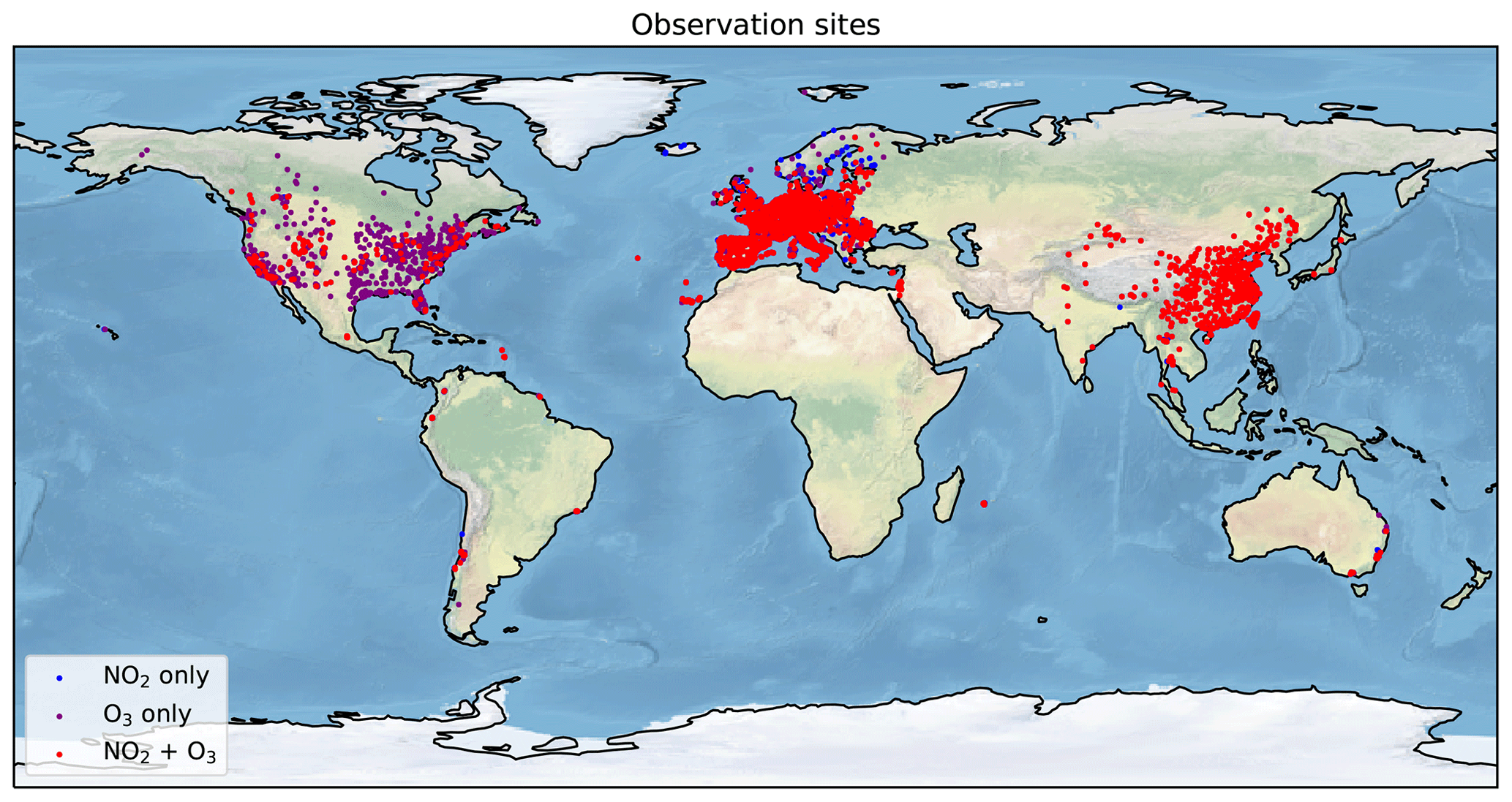
Figure 1Location of the 5756 observation sites included in the analysis. Red points indicate sites with both NO2 and O3 observations (3485 in total), purple points show locations with O3 observations only (978 sites), and blue points show locations with NO2 observations only (1293 sites). See the Appendix for detailed maps for North America, Europe, and China.
Table 1Observational data sources used in the analysis. Time period covers 1 January 2018–1 July 2020.
2.2 Model
Meteorological and atmospheric chemistry information at each of the air quality observation sites is obtained from the NASA Goddard Earth Observing System Composition Forecast (GEOS-CF) model (Keller et al., 2020). GEOS-CF integrates the GEOS-Chem atmospheric chemistry model (v12-01) into the GEOS Earth System Model (Long et al., 2015; Hu et al., 2018) and provides global hourly analyses of atmospheric composition at 25×25 km2 spatial resolution, available in near-real time at https://gmao.gsfc.nasa.gov/weather_prediction/GEOS-CF/data_access/, last access: 5 July 2020 (Knowland et al., 2020). Anthropogenic emissions are prescribed using monthly Hemispheric Transport of Air Pollution (HTAP) bottom-up emissions (Janssens-Maenhout et al., 2015), with imposed weekly and diurnal scale factors as described in Keller et al. (2020). The same anthropogenic base emissions are used for the years 2018–2020. Therefore, GEOS-CF does not account for any anthropogenic emission changes since 2018, notably any anthropogenic emission reductions related to COVID-19 restrictions. However, it does capture the variability in natural emissions such as wildfires (based on the Quick Fire Emissions Dataset, QFED) (Darmenov and Da Silva, 2015) or lightning and biogenic emissions (Keller et al., 2014). While the meteorology and stratospheric ozone in GEOS-CF are fully constrained by pre-computed analysis fields produced by other GEOS systems (Lucchesi, 2015; Wargan et al., 2015), no trace gas observations are directly assimilated into the current version of GEOS-CF. It thus provides a “business-as-usual” estimate of NO2 and O3 that can be used as a baseline for input into the meteorological normalization process.
2.3 Machine learning bias correction
2.3.1 Overall strategy
We use the XGBoost machine learning algorithm (https://xgboost.readthedocs.io/en/latest/#, last access: 15 March 2020) (Chen and Guestrin, 2016; Frery et al., 2017) to develop a machine learning model to predict the time-varying bias at each observation site at an hourly scale. XGBoost uses the Gradient Boosting framework to build an ensemble of decision trees, trained iteratively on the residual errors to improve the model predictions in a stagewise manner (Friedman, 2001). Based on the 2018–2019 observation–model differences, the machine learning model is trained to predict the systematic (recurring) model bias between hourly observations and the co-located model predictions. These biases can be due to errors in the model, such as emission estimates, sub-grid-scale local influences (representational error), or meteorology and chemistry. Since model biases are often site-specific, we train a separate machine learning model for each site.
The design of the XGBoost framework is determined by a set of hyperparameters, such as the learning rate, maximum tree depth, or minimum loss reduction. While a full hyperparameter optimization across all sites – e.g., by using a grid search approach – would be computationally prohibitive, we conducted hyperparameter sensitivity tests at few selected sites and found that the XGBoost performance only improved marginally at these sites when using hyperparameters other than the model defaults (less than 5 % improvement). In addition, we found that the sites respond differently to the same change in hyperparameter setup, suggesting that there is no uniform hyperparameter design that is optimal across all sites. Based on this, we chose to use the default XGBoost model parameters at all locations, with a learning rate of 0.3, minimum loss reduction of 0, maximum tree depth of 6, and L1 and L2 regularization terms of 0 and 1, respectively.
For each location, we split the 2-year training dataset into eight quarterly segments (January–March, April–June, etc.) and train the model eight times, each time omitting one of the segments (8-fold cross validation). The omitted segment is used as test data to validate the general performance of the machine learning model and to provide an uncertainty estimate, as is further discussed below. This approach aims to reduce the auto-correlation signal that can lead to overly optimistic machine learning results (Kleinert et al., 2021), while still including data from all four seasons in the testing. Once trained, the final model prediction at each location consists of the average prediction of the eight models.
The observations used in this analysis are not always quality-controlled, which can cause issues if erroneous observations are included in the training, such as unrealistically high O3 concentrations of several thousand parts per billion by volume. As an ad hoc solution to this problem, we remove all observations below or above 2 standard deviations from the annual mean from the analysis. Sensitivity tests using more stringent thresholds of 3 or even 4 standard deviations resulted in no significant change in our results.
2.3.2 Evaluation of model predictors
The input variables fed into the XGBoost algorithm are provided in Table A1. The input features encompass 9 meteorological parameters (as simulated by the GEOS-CF model: surface northward and eastward wind components, surface temperature and skin temperature, surface relative humidity, total cloud coverage, total precipitation, surface pressure, and planetary boundary layer height), modeled surface concentrations of 51 chemical species (O3, NOx, carbon monoxide, volatile organic compounds (VOCs), and aerosols), and 21 modeled emissions at the given location. In addition, we provide as input features the hour of the day, day of the week, and month of the year; these allow the machine learning model to identify systematic observation–model mismatches related to the diurnal, weekly, and seasonal cycle of the pollutants. In addition, for sites with observations available for the full two years, we provide the calendar days since 1 January 2018 as an additional input feature to also correct for inter-annual trends in air pollution, e.g., due to a steady decrease in emissions not captured by the model. This follows a similar technique to Ivatt and Evans (2020) and Petetin et al. (2020).
Gradient-boosted tree models consist of a tree-like decision structure, which can be analyzed to understand how the model uses the input features to make a prediction. Particularly useful in this context is the SHapely Additive exPlanations (SHAP) approach, which is based on game-theoretic Shapely values and represents a measure of each feature's responsibility for a change in the model prediction (Lundberg et al., 2017). SHAP values are computed separately for each individual model prediction, offering detailed insight into the importance of each input feature to this prediction while also considering the role of feature interactions (Lundberg et al., 2020). In addition, combining the local SHAP values offers a representation of the global structure of the machine learning model.
Figure A4 shows the distribution of the SHAP values for all NO2 predictors separated by polluted sites (left panel) and non-polluted sites (right panel), with polluted sites defined as locations with an annual average NO2 concentration of more than 15 ppbv. Generally, the model-predicted (unbiased) NO2 concentration is the most important predictor for the model bias, followed by the hour of the day, the day since 1 January 2018 (“trendday”), and a suite of meteorological variables including wind speed (u10m, v10m), planetary boundary hight (zpbl), and specific humidity (q10m). All of these factors are expected to highly impact NO2 concentrations and it is thus not surprising that the model biases are most sensitive to them. While there is considerable spread in the feature importance across the individual sites, there is little overall difference in the feature ranking between polluted vs. non-polluted sites.
Figure A5 shows the SHAP value distribution for all O3 predictors, again separated into polluted and non-polluted sites (using the same definition as for the NO2 sites). Unlike for NO2, the bias-correction models for polluted sites exhibit different feature sensitivities than the non-polluted sites. At polluted locations, the availability of reactive nitrogen (NO2, NOy, PAN) is the dominant factor for explaining the model O3 bias, reflecting the tight chemical coupling between NOx and O3 (Seinfeld and Pandis, 2016). This is followed by the month of the year, total precipitation (tprec), and O3 concentration, again variables that are expected to be correlated to O3. At non-polluted sites, the uncorrected O3 concentration is on average the most relevant input feature for the bias correctors, followed by the month of the year and the odd oxygen concentration (). The non-polluted sites are generally more sensitive to wind speed, reflecting the fact that O3 production and loss at these locations is less dominated by local processes compared to the polluted sites.
2.3.3 Machine learning model skill scores
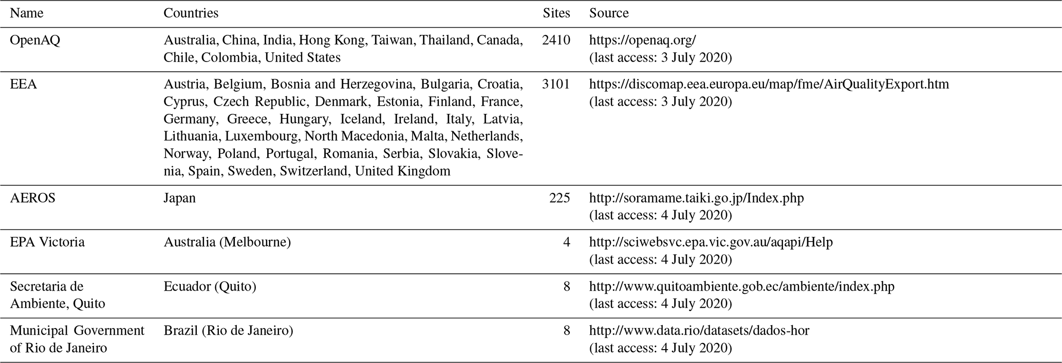
Figures 2 and 3 summarize the machine learning model statistics for NO2 and O3, respectively. The normalized mean bias (NMB), normalized root-mean-square error (NRMSE), and Pearson correlation coefficient (R) at each site are shown for both the training (blue) and the test (red) dataset. We define NMB as mean bias normalized by average concentration at the given site, and the NRMSE as the root-mean-square error normalized by the range of the 95th percentile concentration and 5th percentile concentration. Rather than using the mean as the denominator for the NRMSE, we choose the percentile window as a better reference point for the concentration variability at a given site. Using the mean as the denominator for the NRMSE would lead to very similar qualitative results.
For both NO2 and O3, the bias-corrected model predictions show no bias when evaluated against the training data, NRMSEs of less than 0.3, and correlation coefficients between 0.6–1.0 (NO2) and 0.75–1.0 (O3). Compared to the training data, the skill scores on the test data show a higher variability, with an average NMB of −0.047 for NO2 and −0.034 for O3, a NRMSE of 0.25 (NO2) and 0.18 (O3), and a correlation of 0.64 (NO2) and 0.84 (O3). We find no significant difference in skill scores between background vs. polluted sites or different countries.
A number of factors likely contribute to the poorer statistical results at some of the sites. Importantly, some sites might be prone to overfitting if the training data include events that are not easily generalizable, such as unusual emission activity (e.g., biomass burning, fireworks, closure of nearby point source) or weather patterns that are not frequently observed. In addition, the availability of test data at some locations is weak (less than 50 %), which can contribute to a poorer skill score.
2.3.4 Uncertainty estimation
To quantify the uncertainty of an individual model predictions at any given site, we use the standard deviation of the model-observation differences on the test data. For sites with 100 % test data coverage, this represents the standard deviation from a sample of 17 520 hourly model-observation pairs. The thus obtained individual NO2 prediction uncertainties range between 3.9–28 ppbv (mean = 8.5 ppbv) at polluted sites and 0.1–18 ppbv at clean sites (average of 4.9 ppbv). On a relative basis, this corresponds to an average uncertainty of 45 % at polluted sites and 65 % at clean sites. For O3, we obtain an average individual prediction uncertainty of 14 ppbv (4.6–33 ppbv) at polluted sites and 9.0 ppbv (2.8–45 ppbv) at clean sites, corresponding to an average relative uncertainty of an individual prediction of 29 % and 33 % at polluted and clean sites, respectively.
The results presented in this paper are averages aggregated over multiple hours and locations, and the reported uncertainties are adjusted accordingly by calculating the mean uncertainty from the above-described hourly uncertainties σi:
This assumes that the errors across individual sites are uncorrelated. The error covariance across sites is complex: two urban sites close to each other might show a low degree of error correlation due to local-scale (street, canyon, etc.) differences, whereas two background sites further apart might show significantly more correlation due to regional-scale (synoptic) processes. In addition, our uncertainty calculation also implies that the aggregated mean error approaches zero. Given that the average mean biases of the machine learning models are clustered around zero (Figs. 2 and 3), this is a valid general assumption – especially when aggregating across multiple sites. For simplicity we keep the current analysis but acknowledge that it might lead to overly optimistic uncertainty estimates for sites with a relatively large mean bias.
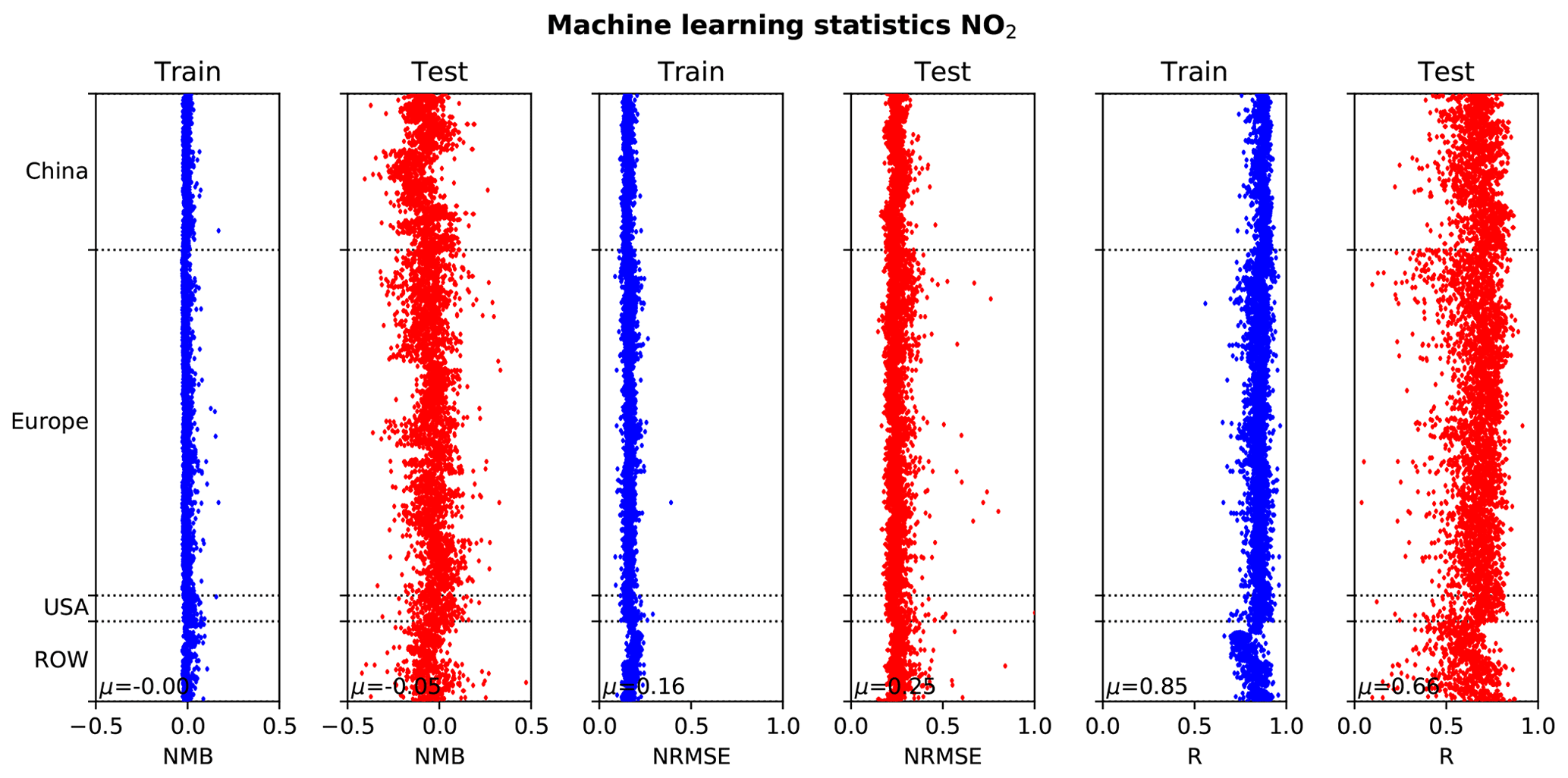
Figure 2Machine learning statistics between hourly observations and the corresponding bias-corrected model predictions for each observation location. Shown are the normalized mean bias (NMB), normalized root-mean-square error (NRMSE), and Pearson correlation coefficient (R) for the training data (blue) and the test data (red). Data are sorted by region: China, Europe, United States (USA), and rest of the world (ROW). The mean values across all locations are shown in the figure inset.
2.4 Lockdown dates
To support interpretation and guide visualizations, we include approximate national lockdown dates in all figures. The start and end dates for these are from https://en.wikipedia.org/wiki/COVID-19_pandemic_lockdowns, last access: 1 July 2020 (as of 1 July 2020) or based on local knowledge, with the full list of start and end dates given in Table A2. It should be noted that in many countries lockdown policy varied regionally and that many locations enacted “soft” stay-at-home orders before the official lockdowns. Human behavior is therefore expected to have changed considerably in many locations before the official lockdowns went into force.
3.1 Nitrogen dioxide
Figure 4 shows the weekly mean observations of NO2 concentration, the GEOS-CF estimate, and the BCM prediction based on the machine learning predictor trained on 2018–2019 for the five cities of Wuhan (China), Taipei (Taiwan), Milan (Italy), New York (USA), and Rio de Janeiro (Brazil) from January 2018 through June 2020. We choose these five cities for illustration as they represent a diverse level of socio-economic development and due to the cities' variable responses to the COVID-19 pandemic. These five cities are also illustrative of the varying quality of the uncorrected GEOS-CF predictions compared to the observations. For example, as shown by the dashed grey lines vs. the solid black lines in Fig. 4, the uncorrected model predictions are in good agreement with observations in Rio de Janeiro but underestimate the observed NO2 concentrations in Taipei and Milan while overestimating concentrations over New York. These differences are a combination of the observation–model scale mismatch (25×25 km2 vs. point observation) and model errors, such as the simulated spatiotemporal distribution of NOx emissions or the modeling of the local boundary layer. The model–observation mismatch is particularly pronounced for Wuhan, where the model does not capture the observed seasonal cycle, pointing to errors in the imposed seasonal cycle of NOx emissions in the model.
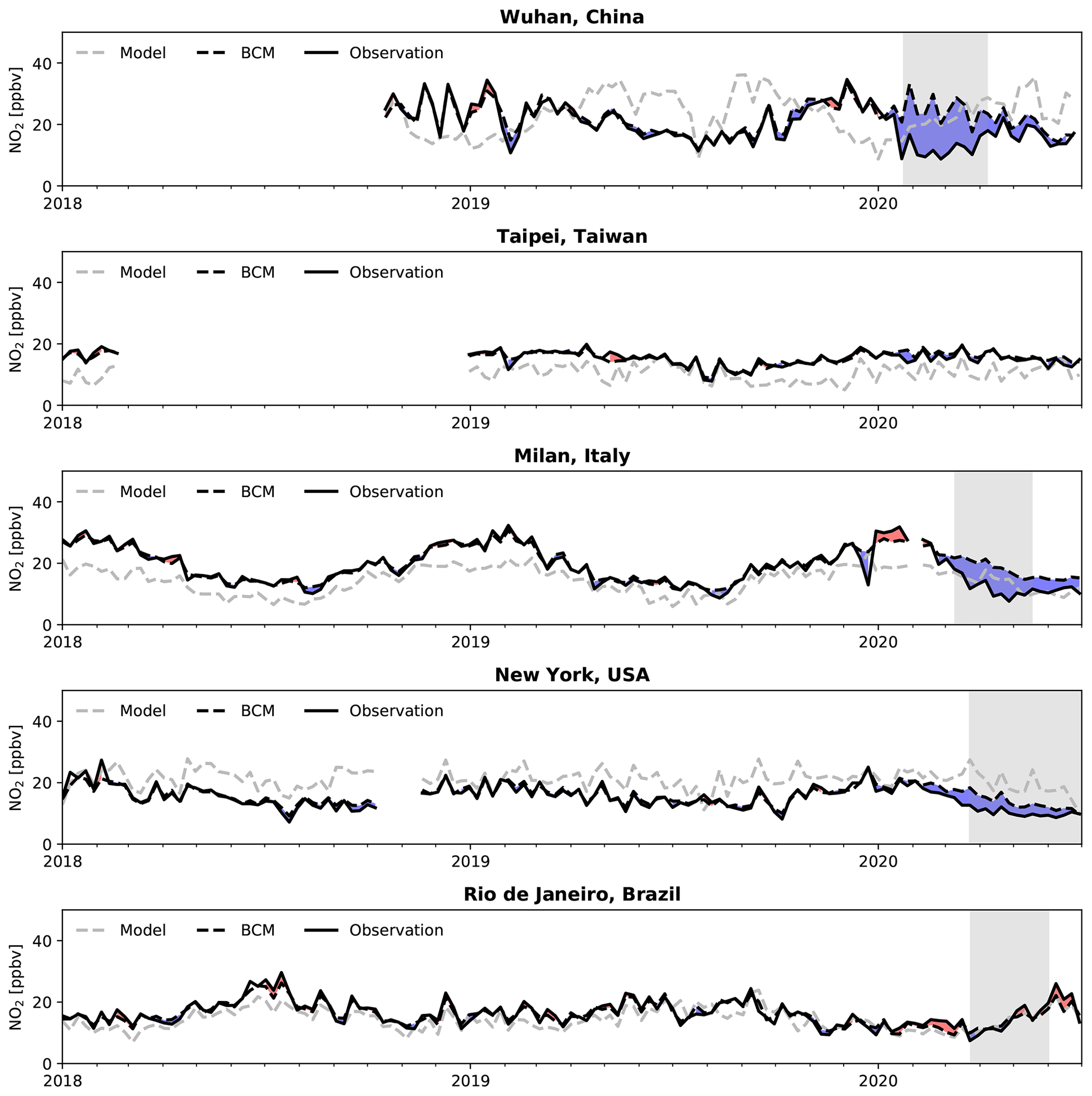
Figure 4Comparison of NO2 surface concentrations (ppbv = nmol mol−1) for Wuhan, Taipei, Milan, New York, and Rio de Janeiro for January 2018 through June 2020. Observed values are shown in solid black, the original GEOS-CF model simulation is shown in dashed grey, and the BCM predictions are in dashed black. The area between observations and BCM predictions is shaded blue (red) if observations are lower (higher) than BCM predictions. Grey areas represent the period of lockdown. Shown are the 7 d average mean values for the 9, 18, 19, 14, and 2 observational sites in Wuhan, Taipei, Milan, New York, and Rio de Janeiro, respectively. Observations for China are only available starting in mid-September 2018.
In contrast to the uncorrected model predictions, the BCM closely follows the observations for years 2018 and 2019 (dashed black lines in Fig. 4). The grey region in Fig. 4 shows the start and end of the implementation of COVID-19 containment measures. Once containment is implemented, observed concentrations start to diverge from the BCM prediction for Wuhan, Milan, and New York (Fig. 4). For Wuhan, we find a reduction in NO2 of 54 (48–59) % relative to the expected BCM value for February and March 2020, and average decreases of 30 %–40 % are found over Milan (24 %–43 %) and New York (20 %–34 %) starting in mid-March and lasting through April (Fig. 4; Tables A3–A5). For cities where restrictions have been mainly removed (Wuhan, Milan) concentrations rise back towards the BCM value, although the concentrations in neither city have been fully restored to what might be expected based on the business-as-usual GEOS-CF simulation.
Looking more broadly at cities around the globe, 53 of the 64 specifically analyzed cities feature NO2 reductions of between 20 %–50 % (Figs. A6–A8 and Tables A3–A5). Most locations issued social distancing recommendations prior to the legal lockdowns and observed NO2 declines often precede the official lockdown date by 7–14 d (e.g., Brussels, London, Boston, Phoenix, and Washington, D.C.).
For Taipei and Rio de Janeiro, the observations and the BCM show little difference (Fig. 4), consistent with the less stringent quarantine measures in these places. Other cities with only short-term NO2 reductions of less than 25 % include Atlanta (USA), Prague (Czech Republic), and Melbourne (Australia), again fitting with the comparatively relaxed containment measures in these places (Figs. A6–A8). In contrast, Tokyo (Japan) and Stockholm (Sweden), which also implemented a less aggressive COVID-19 response, exhibit NO2 reductions comparable to those of cities with official lockdowns (>20 %), suggesting that economic and human activities were similarly subdued in those cities.
Substantial differences exist between cities in South America, with Rio de Janeiro and Santiago de Chile showing little change over the analyzed period, whereas Quito (Ecuador) and Medellín (Colombia) experienced a greater than 50 % reduction in NO2 after the initiation of strict restrictions measures in mid-March (Fig. A8 and Table A5). Concentrations in Medellín rebounded sharply in April and May, while concentrations in Quito remained 55 (52–58) % below business as usual throughout May and only started to return back to normal in June.
To evaluate the large-scale impact of COVID-19 restrictions on air quality, we aggregate the individual observation–model comparisons by country. We note that our estimates for some countries (e.g., Brazil, Colombia) are based on a single city and likely not representative of the whole country. On a country level, we find the sharpest and earliest drop in NO2 over China, where observed concentrations fell, on average, 55 (51–59) % below their expected value in early February when restrictions were implemented (Fig. 5). Concentrations remained at this level until late February, at which point they started to increase until restrictions were significantly relaxed in early April. Our analysis suggests that Chinese NO2 concentrations have recovered to within 5 (1–9) % of the business-as-usual values since then. For 2019 (dashed line in Fig. 5) the BCM shows a reduction in NO2 concentrations around Chinese New Year (5 February 2019), and it is likely that some reduction around the equivalent 2020 period (25 January 2020) would have occurred anyway. However, the 2020 reductions are significantly larger and more prolonged than in 2019. Similar to China, India shows large reductions in NO2 concentration (58 (49–67) %) coinciding with the implementation of restrictions in mid-March (Fig. 5); however, NO2 concentrations have not yet recovered by the end of June, reflecting the prolonged duration of lockdown measures. Other areas of Asia, such as Hong Kong and Taipei, implemented smaller restrictions than China or India and they show significantly smaller decreases (less than 20 %).
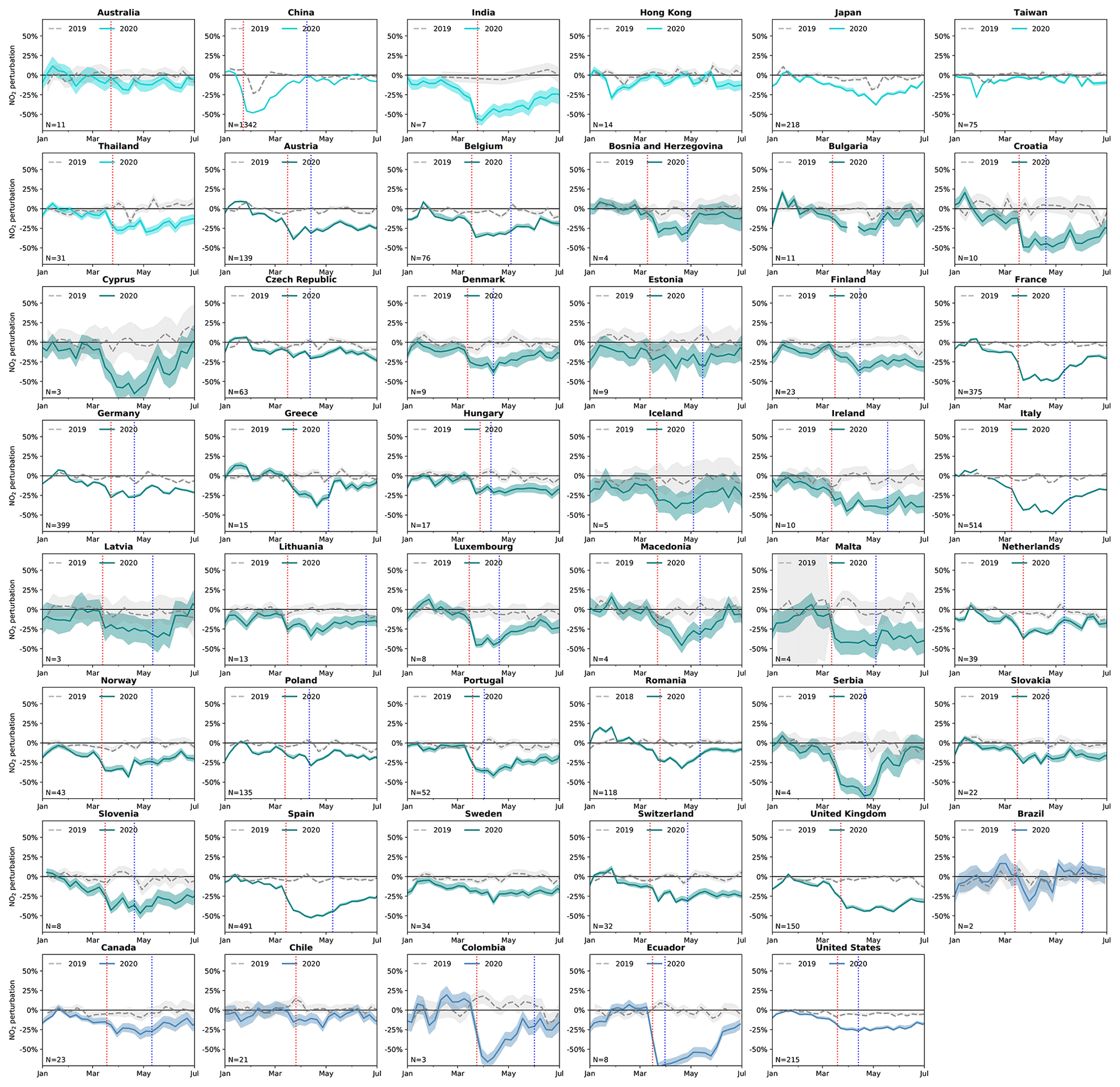
Figure 5The 7 d average fractional difference between observed NO2 and the BCM predictions for 46 countries between 1 January through 30 June, aggregated from all sites across each country (number of sites given at the bottom left of each panel). The thick line indicates the mean across all sites for the first half of 2020, with the shaded area representing the uncertainty estimate. Differing colors indicate differing regions (cyan: Asia and Australia; green: Europe; blue: Americas). The dashed grey line indicates the equivalent average for the same 6 month period in 2019 (note that 2019 data was included in the training). The dashed vertical red line indicates COVID-19 restriction dates, and the blue line indicates the beginning of easing measures.
For Europe and the United States, we find widespread NO2 reductions averaging 22 (19–25) % in March and 33 (30–36) % in April (Fig. 5). In some countries, recovery is evident as lockdown restrictions are removed or lessened (e.g., Greece, Romania), but in 29 out of 36 countries concentrations remain 20 % or more below the business-as-usual scenario throughout May and June.
3.2 Ozone
We follow the same methods for developing a business-as-usual counterfactual for O3 as we did for NO2 in Sect. 3.1. Any change in local O3 concentration arising from COVID-19 restrictions is set against a large seasonal increase in (background) concentrations in the Northern Hemisphere springtime (Fig. 6). Due to the longer atmospheric lifetime of O3 compared to NO2, the local O3 signal is expected to be comparatively small. This makes attributing changes in O3 concentration more challenging than for NO2. Our analysis shows an O3 increase of up to 50 % for some periods in cities with large NO2 reductions (e.g., Wuhan, Milan, Quito; Figs. 3 and A9–A11), but there is much less convincing evidence for a systematic O3 response across cities or on a regional level (Fig. 7). For example, our analysis shows little O3 difference in Beijing and Madrid during lockdown despite NO2 declines comparable to Wuhan or Milan (Figs. A9–A11). O3 enhancements of up to 20 % are found over Europe (e.g., Belgium, Luxembourg, Serbia), with a peak in early April, approximately 2 weeks after lockdown started (Fig. 7).

Figure 6Comparison of O3 surface concentrations for Wuhan, Taipei, Milan, New York, and Rio de Janeiro for January 2018 through June 2020. Observed values are shown in solid black, the original GEOS-CF model simulation is shown in dashed grey, and the BCM predictions are in dashed black. The area between observations and BCM predictions is shaded blue (red) if observations are lower (higher) than BCM predictions. The grey areas represent the period of lockdown. Shown are the 7 d average mean values for the 9, 18, 19, 14, and 4 observational sites in Wuhan, Taipei, Milan, New York, and Rio de Janeiro, respectively. Observations for China are only available starting in mid-September 2018.
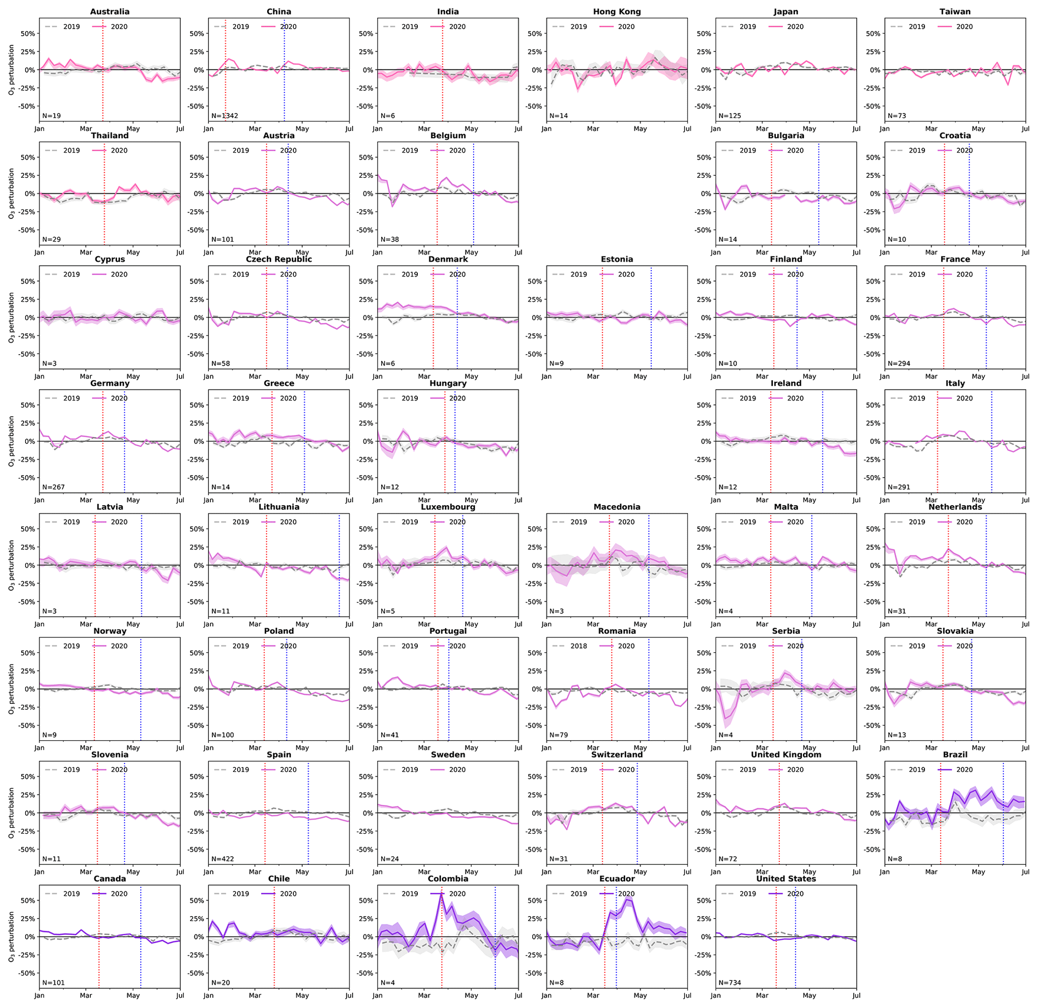
Figure 7Similar to Fig. 5 but for O3 and without Bosnia and Herzegovina and Iceland. Differing colors indicate differing regions (pink: Asia and Australia; light purple: Europe; dark purple: Americas).
The analysis of O3 is complicated by its nonlinear chemical response to NOx emissions. In the presence of sunlight, O3 is produced chemically from the oxidation of volatile organic compounds in the presence of NOx (Seinfeld and Pandis, 2016). Therefore, a decline in NOx emissions could decrease O3 production and thus suppress O3 concentrations. On the other hand, the process of NOx titration, in which freshly emitted NO rapidly reacts with O3 to form NO2, acts as a sink for O3 (Seinfeld and Pandis, 2016). Odd oxygen (Ox) is conserved when O3 reacts with NO and thus offers a tool for separating these competing processes. Figure 8 presents the global mean diurnal cycle for O3 and Ox for the 5-month period since 1 February 2020 for both the observations and the BCM model, based on the individual hourly predictions at each observation site aggregated by local hour. The analysis of O3 and Ox is based on the same set of observation sites where both NO2 and O3 observations are available (see Fig. 1). Compared to the BCM model, there has been an increase in the concentration of nighttime O3 (00:00–05:00 LT, local time, Fig. 8a) by 1 ppbv (ppbv = nmol mol−1) compared to the BCM, whereas Ox shows a decrease of 1 ppbv (Fig. 8b). While these changes are small in magnitude, they represent a multi-month aggregate over 3485 observation sites that are statistically significant at the 1 % confidence interval. It should be noted that the biases of the machine learning models show little diurnal variability (Figs. A12–13), suggesting that this result is not caused by poor model performance during specific times of the day.
Our results indicate that during the night reduced NO emissions led to a reduction in O3 titration, allowing O3 concentrations to increase. During the afternoon, we find that O3 concentrations are lower by 1 ppbv (Fig. 8a), while observed Ox concentrations are lower than the baseline model by almost 2 ppbv at 14:00 LT (Fig. 8b). We attribute the lower Ox to reduced net Ox production due to the lower NOx concentration, but as titration is also reduced, daytime O3 concentrations change little. Overall changes to mean O3 concentrations are small, but there is a flattening of the diurnal cycle.
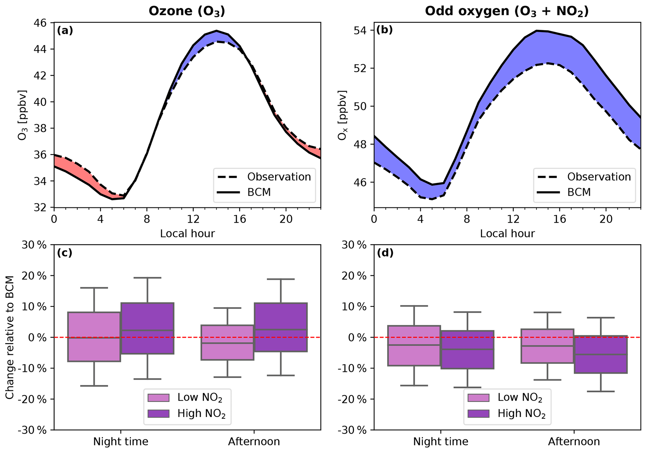
Figure 8Observed and BCM-modeled diurnal cycle of O3 (a) and Ox (b) averaged across all surface observation sites between 1 February 2020 through 30 June 2020 with estimated corresponding changes in surface O3 (c) and Ox (d) relative to the BCM. Bar plots (c and d) show observed changes during nighttime (0:00–05:00 LT) and the afternoon (12:00–17:00 LT) for locations with low (<15 ppbv) and high (>15 ppbv) NO2 concentrations (based on the 2019 average).
As shown in the lower panels in Fig. 8, both factors – enhanced nighttime O3 and reduced daytime Ox – are more pronounced at locations where preexisting NO2 concentrations are high (>15 ppbv). This suggests that the observed O3 deviations from the BCM are indeed coupled to NOx reductions due to COVID-19 restrictions, given that those are most pronounced at polluted sites.
3.3 NOx emission reductions
The NO2 analysis presented in Sect. 3.1 implies a stark reduction in NOx emissions. However, due to the impact of atmospheric chemistry, changes in NO2 concentrations do not reflect the same relative change in NOx emissions. Because of this, the NO2 NOx ratio and the NOx lifetime, both of which depend on seasonality and the local chemical environment, need to be taken into account when inferring NOx emissions from NO2 concentrations (Lamsal et al., 2011; Shah et al., 2020). To estimate the relationship between changes in NOx emission and changes in NO2 concentrations, we conducted a sensitivity simulation for the time period 1 December 2019 to 8 June 2020 using the GEOS-CF model with perturbed anthropogenic emissions. The perturbation simulation uses anthropogenic NOx emissions scaled based on adjustment factors derived from NO2 tropospheric columns observed by the NASA OMI instrument (Boersma et al., 2011). Daily scale factors were computed by normalizing coarse-resolution (2×2.5∘) 14 d NO2 tropospheric column moving averages by the corresponding moving average for year 2018 (the emissions base year in GEOS-CF; Sect. 2.2). Forest fire signals were filtered out based on QFED emissions and no scaling was applied over water. This results in anthropogenic emission adjustment factors of 0.3 to 1.4 (Fig. A14), comparable to the magnitude obtained from the observation–BCM comparisons at cities globally (Fig. 5) and capturing the range of expected NOx emission changes. However, it should be noted that the scale factors do not necessarily coincide in space and time with the ones derived from observations and the BCM, and they do not include any adjustment for the NO2 NOx ratio.
Figure 9a shows the response of NO2 surface concentration to a change in NOx emissions derived from the comparison of the sensitivity experiment against the GEOS-CF reference simulation. Our results indicate that NO2 concentrations drop, on average, by 80 % of the fractional decrease in anthropogenic NOx emission, with a further diminishing effect for emission reductions greater than 50 %. This reflects both the buffering effect of atmospheric chemistry and the presence of natural background NO2. The here-derived average sensitivity of 0.8 between a change in surface NO2 to a change in NOx emissions is comparable to the value of 0.86 () obtained by Lamsal et al. (2011) for the relationship between NOx emissions and tropospheric column NO2 observations.
To infer the reduction in anthropogenic NOx emissions due to COVID-19 containment measures during the first 6 months of 2020, we use the best linear fit between the simulated NOx NO2 sensitivity (dashed purple line in Fig. 9a). To do so, we calculate the monthly percentage emission change at each observation site based on the NO2 anomalies derived in Sect. 3.1 and the corresponding best fit NOx NO2 sensitivity (Fig. 9a). This is a simplification, as the local NOx NO2 sensitivity ratio is highly dependent on the local environment. To account for this uncertainty, we assign an absolute error of 15 % to our NOx NO2 sensitivity, as derived from the spread in the NOx NO2 ratio in the sensitivity simulation (Fig. 9a). We then aggregate these estimates to a country level by weighting them based on average NO2 concentrations per location, thus giving higher weight to locations with more nearby NOx emission sources. It should be noted that for some countries our estimates are based upon a small number of observation sites that might not be representative for the country as a whole. This is particularly true for India and Brazil, where less than 10 observation sites are available. While the smaller observation sample size is reflected in the wider uncertainty associated with these emission estimates compared to countries with a much denser monitoring network (e.g., China or Europe), the applied extrapolation method might incur errors that are not reflected in the stated uncertainty ranges.
To obtain absolute estimates in emission changes, the monthly country-level percentage emission changes are convoluted with bottom-up emissions estimates for 2015 from the Emission Database for Global Atmospheric Research (EDGAR v5.0_AP; Crippa et al., 2018, 2020). The choice of EDGAR v5.0 as the bottom-up reference inventory (over, e.g., the HTAP emissions inventory used in GEOS-CF) was motivated by the fact that its baseline has been updated more recently and the country emission totals – which our analysis is based on – are readily available.
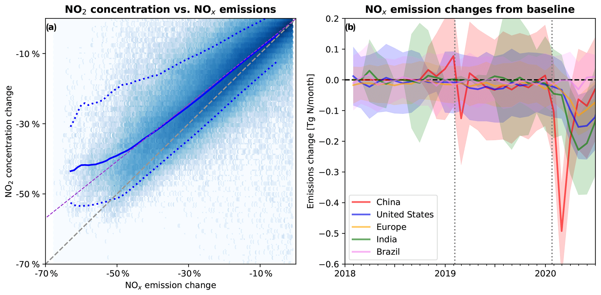
Figure 9(a) Response of NO2 surface concentration (y axis) to a change in NOx emissions (x axis), as deduced from a model sensitivity simulation (see methods). The solid blue line shows the mean value across all individual grid cells (blue squares) and the dotted blue lines show the 5 % and 95 % quantiles. The dashed purple line shows the best linear fit. (b) Estimated monthly change in NOx emissions from the baseline since 2018 for China (red), the United States (blue), Europe (yellow), India (green), and Brazil (purple), as estimated from observed NO2 concentration anomalies. Shaded areas indicate estimated emission uncertainties. Dotted grey lines indicate Chinese New Year 2019 and 2020.
As summarized in Table 2, we calculate that the total reduction in anthropogenic NOx emissions due to COVID-19 containment measures during the first 6 months of 2020 amounted to 3.1 (2.6–3.6) TgN (Fig. 9b and Table 2). This is equivalent to 5.5 (4.7–6.4) % of global annual anthropogenic NOx emissions (Table 2). Our estimate encompasses 46 countries that together account for 67 % of the total emissions (excluding international shipping and aviation). We have no information for significant countries such as Russia, Indonesia, or anywhere in Africa due to the lack of publicly available near-real-time air quality information. China accounts for the largest fraction of the total deduced emission reductions (28 %), followed by India (25 %), the United States (18 %), and Europe (12 %).
Table 2Anthropogenic NOx emission reductions in GgN month−1 as derived from NO2 concentration changes.

a EDGAR v5.0_AP 2015 annual emissions expressed as GgN month−1 (Crippa et al., 2020). b Primarily Indonesia, Iran, Mexico, Pakistan, Russia, Saudi Arabia, South Africa, South Korea, and Vietnam. NA: not available.
While our method does not allow for sector-specific emission attribution, we assume our results to be most representative for changes in traffic emissions (rather than say aircraft emissions) given the location of the observation sites. On average, traffic emissions represent 27 % of total anthropogenic NOx emissions (Crippa et al., 2018), and our derived total NOx emission reduction from January–June 2020 corresponds to 21 (17–24) % of global annual traffic emissions. The share of transportation on total NOx emissions is higher in the US and Europe (approx. 40 %) compared to India and China (20 %–25 %). Taking this into account, the derived ratio of NOx emission reductions to annual traffic emissions is 21 (16–26) % in the US, 25 (20–30) % in Europe, 39 (34–44) % in China, and 62 (55–69) % in India.
3.4 Long-term impact of reduced NOx emissions on surface O3
The response of O3 to NO2 declines in the wake of the COVID-19 outbreak is complicated by the competing influences of atmospheric chemistry. From February through June 2020, the diurnal observation-BCM comparisons suggest that the reduction in photochemical production was offset by a smaller loss from titration, as described in Sect. 3.2. This resulted in a flattening of the diurnal cycle and an insignificant net change in surface O3 over a diurnal cycle. The competing impacts of reduced NOx emissions on O3 production and loss are dependent on the local chemical and meteorological environment. This is reflected in the variable geographical response of O3 following the implementation of COVID-19 restrictions (Le et al., 2020; Dantas et al., 2020). Moreover, as atmospheric reactivity increases through the Northern Hemisphere spring and summer, the relative importance of photochemical production is expected to increase in the Northern Hemisphere.
To assess the potential seasonal-scale impact of reduced anthropogenic emissions on O3, we conducted two free-running forecast simulations between 8 June and 31 August 2020, initialized from the GEOS-CF simulation and the sensitivity simulation described in Sect. 3.3, respectively. Both simulations use the same biomass burning emissions based on a historical QFED climatology. For the forecast sensitivity experiment, we assume a sustained, time-invariant 20 % reduction in global anthropogenic emissions of NOx, carbon monoxide (CO), and VOCs. We chose to alter not only the anthropogenic emissions of NOx but also other pollutants whose anthropogenic emissions are highly correlated to NOx, as a reduction in NOx emissions without corresponding declines in CO and VOC emissions seems unrealistic.

Figure 10Change in mean surface O3 over the United States, Europe, and Asia for a sensitivity simulation with altered anthropogenic emissions. The top panels show daily average O3 concentrations at all observation sites within the given region (solid black, January–June), the bias-corrected GEOS-CF model (“BCM”, solid black, 1 January–8 June) continued with a business-as-usual GEOS-CF forecast from 9 June to 31 August, and GEOS-CF forecast assuming sustained 20 % anthropogenic emission reduction (blue). The bottom panels show mean changes in surface O3 for July and August for the low emissions simulation relative to the business-as-usual forecast.
Figure 10 shows the differences between the reference forecast and the sensitivity simulation over the United States, Europe, and China. Our results indicate that sustained lower anthropogenic emissions lead to a general decrease in surface O3 concentrations of 10 %–20 % over eastern China, Europe, and the western and northeastern US during July and August relative to the business-as-usual reference forecast simulation. However, it is also notable that in some locations the model forecast O3 concentrations increase by an equivalent amount (e.g., Scandinavia, southern central US and Mexico, northern India), reflecting the high nonlinearity of atmospheric chemistry. This highlights the complex interactions between emissions, chemistry, and meteorology and their impact on air pollution on different time scales.
The combined interpretation of observations and model simulations using machine learning can be used to remove the confounding effect of meteorology and atmospheric chemistry, offering an effective tool to monitor and quantify changes in air pollution in near-real time. The global response to the COVID-19 pandemic presents a perfect test bed for this type of analysis, offering insights into the interconnectedness of human activity and air pollution. While national mitigation strategies have led to substantial regional NO2 concentration decreases over the past decades in many places (e.g., Hilboll et al., 2013; Russell et al., 2012; Castellanos and Boersma, 2012), the widespread and near-instantaneous reduction in NO2 following the implementation of COVID-19 containment measures indicates that there is still large potential to lower human exposure to NO2 through reduction of anthropogenic NOx emissions.
The here-derived NO2 reductions are in good agreement with other emerging estimates. For instance, we determine an 18 % decline over China for the 20 d after Chinese New Year relative to the preceding 20 d, consistent with the 21 % reduction reported in Liu et al. (2020a). Similarly, our estimated 22 % reduction over China for January to March 2020 is in excellent agreement with the 21 %–23 % reported by Liu et al. (2020b). For Spain, we obtain an NO2 reduction of 46 % between March 14 to 23 April , again in close agreement with the values reported in Petetin et al. (2020).
While large reductions in NO2 concentrations are achievable and immediately follow curtailments in NOx emissions, the O3 response is more complicated and can be in the opposite direction, at times by as much as 50 % (Jhun et al., 2015; Le et al., 2020). The O3 response is dependent on season, timescale, and environment, with an overall tendency to lower surface O3 under a scenario of sustained NOx emission reductions. This shows the complexities faced by policy makers in curbing O3 pollution.
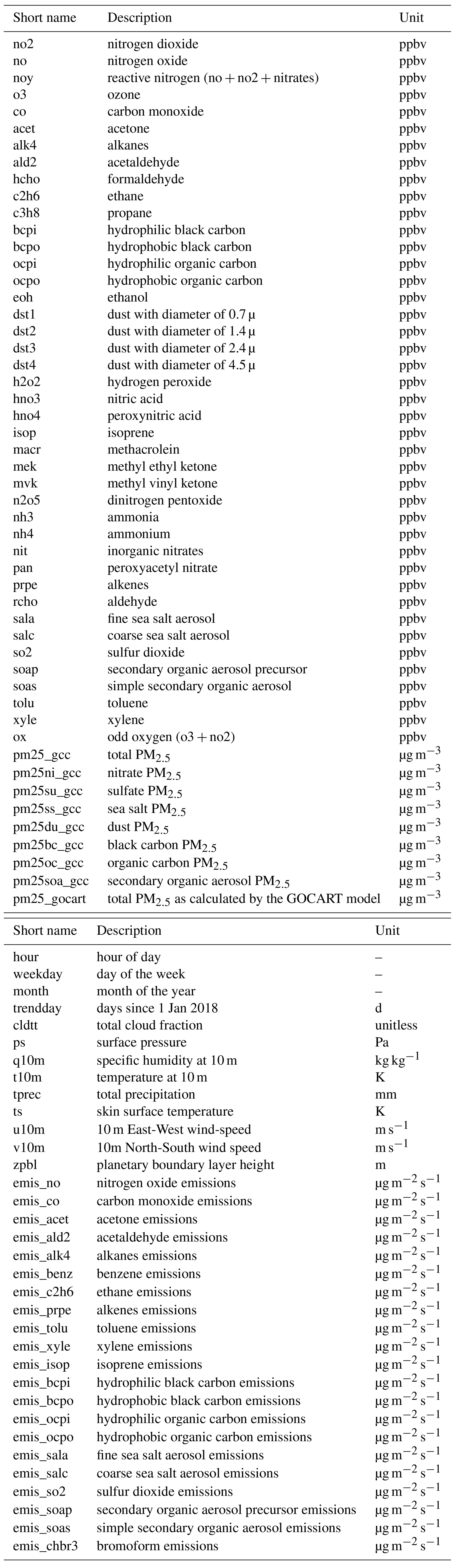

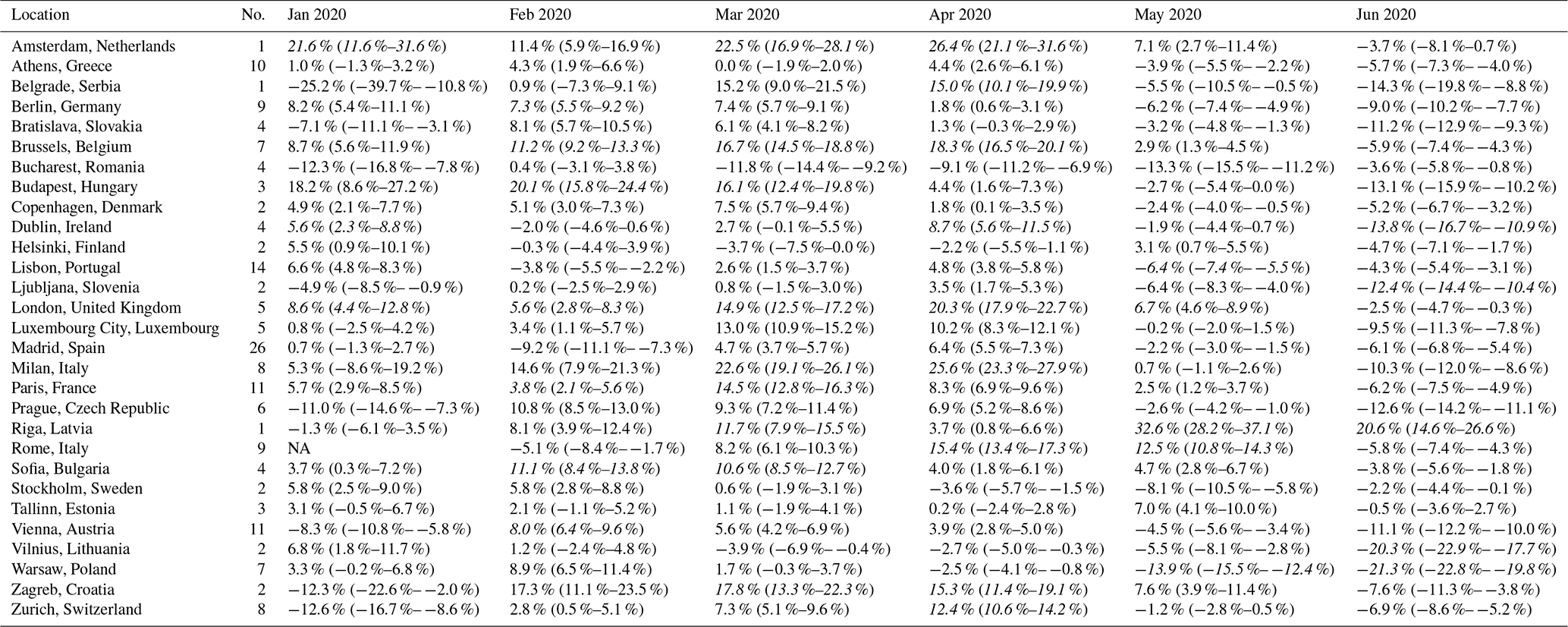
Table A3Monthly changes in NO2 concentrations relative to the bias-corrected model predictions for cities in Asia and Australia. Values in italics denote values that are statistically different from business as usual (p<0.001 based on a Kolmogorov–Smirnov test).
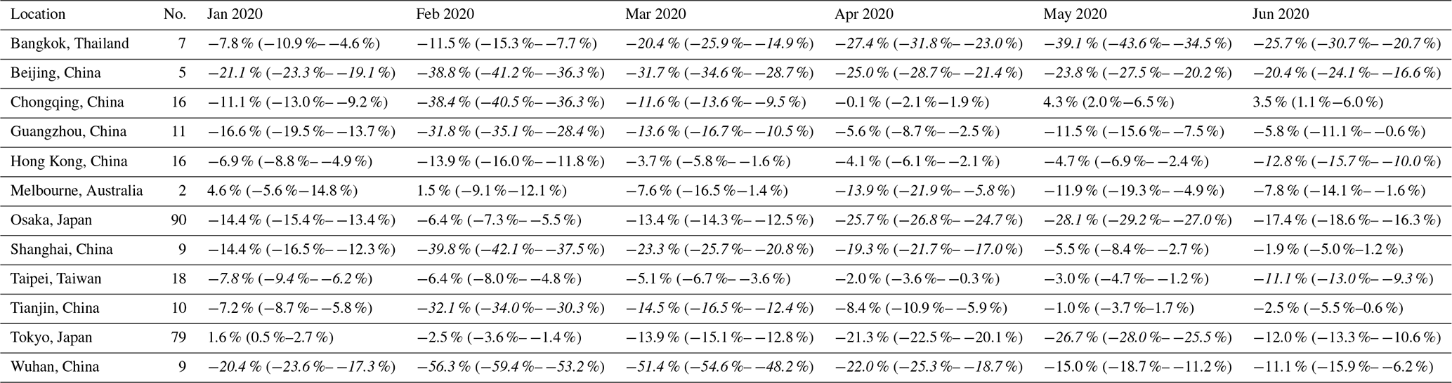
Table A4Monthly changes in NO2 concentrations relative to the bias-corrected model predictions for cities in Europe. Values in italics denote values that are statistically different from business as usual (p<0.001 based on a Kolmogorov–Smirnov test).

NA: not available.
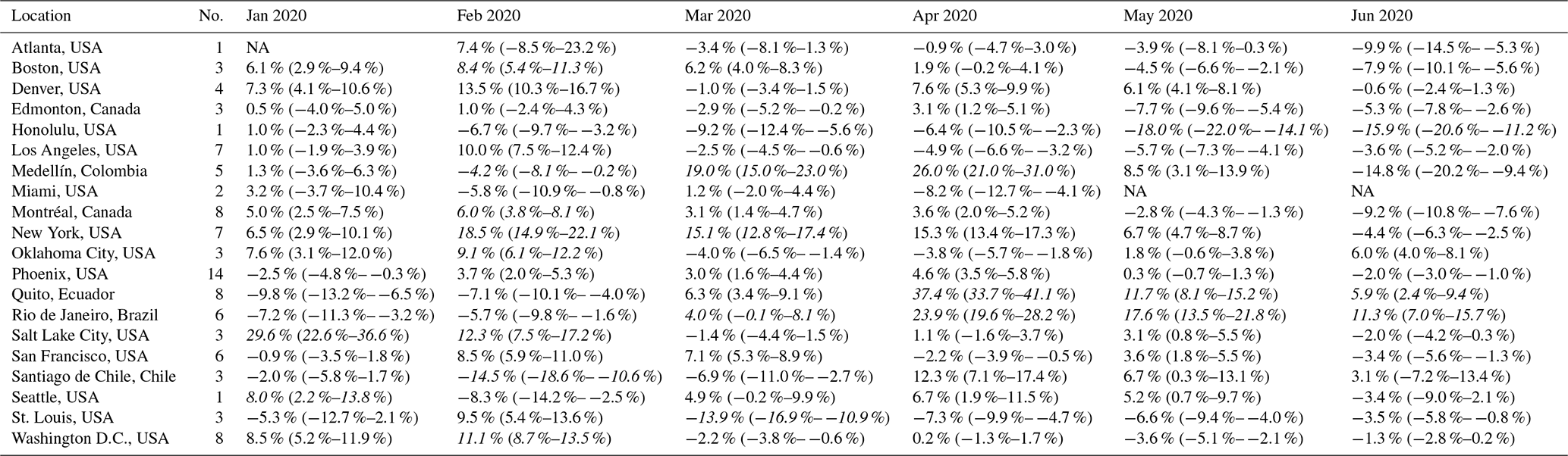
Table A5Monthly changes in NO2 concentrations relative to the bias-corrected model predictions for cities in North America and South America. Values in italics denote values that are statistically different from business as usual (p<0.001 based on a Kolmogorov–Smirnov test).

NA: not available.
Table A6Monthly changes in O3 concentrations relative to the bias-corrected model predictions for cities in Asia and Australia. Values in italics denote values that are statistically different from business as usual (p<0.001 based on a Kolmogorov–Smirnov test).
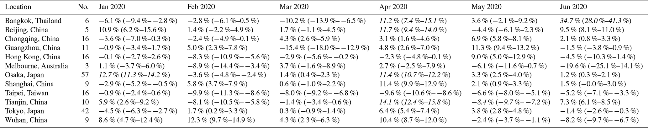
Table A7Monthly changes in O3 concentrations relative to the bias-corrected model predictions for cities in Europe. Values in italics denote values that are statistically different from business as usual (p<0.001 based on a Kolmogorov-Smirnov test).
NA: not available.
Table A8Monthly changes in O3 concentrations relative to the bias-corrected model predictions for cities in North America and South America. Values in italics denote values that are statistically different from business as usual (p<0.001 based on Kolmogorov–Smirnov test).
NA: not available.
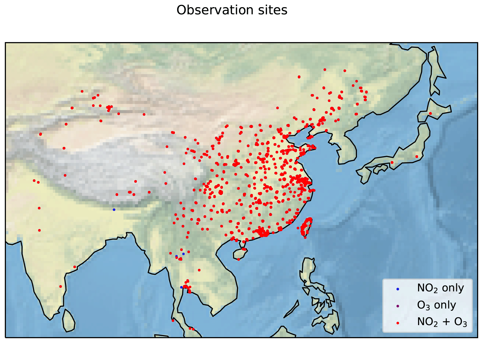
Figure A1Close-up image of Chinese observation sites included in the analysis. Red points indicate sites with both NO2 and O3 observations, purple points show locations with O3 observations only, and blue points show locations with NO2 observations only.
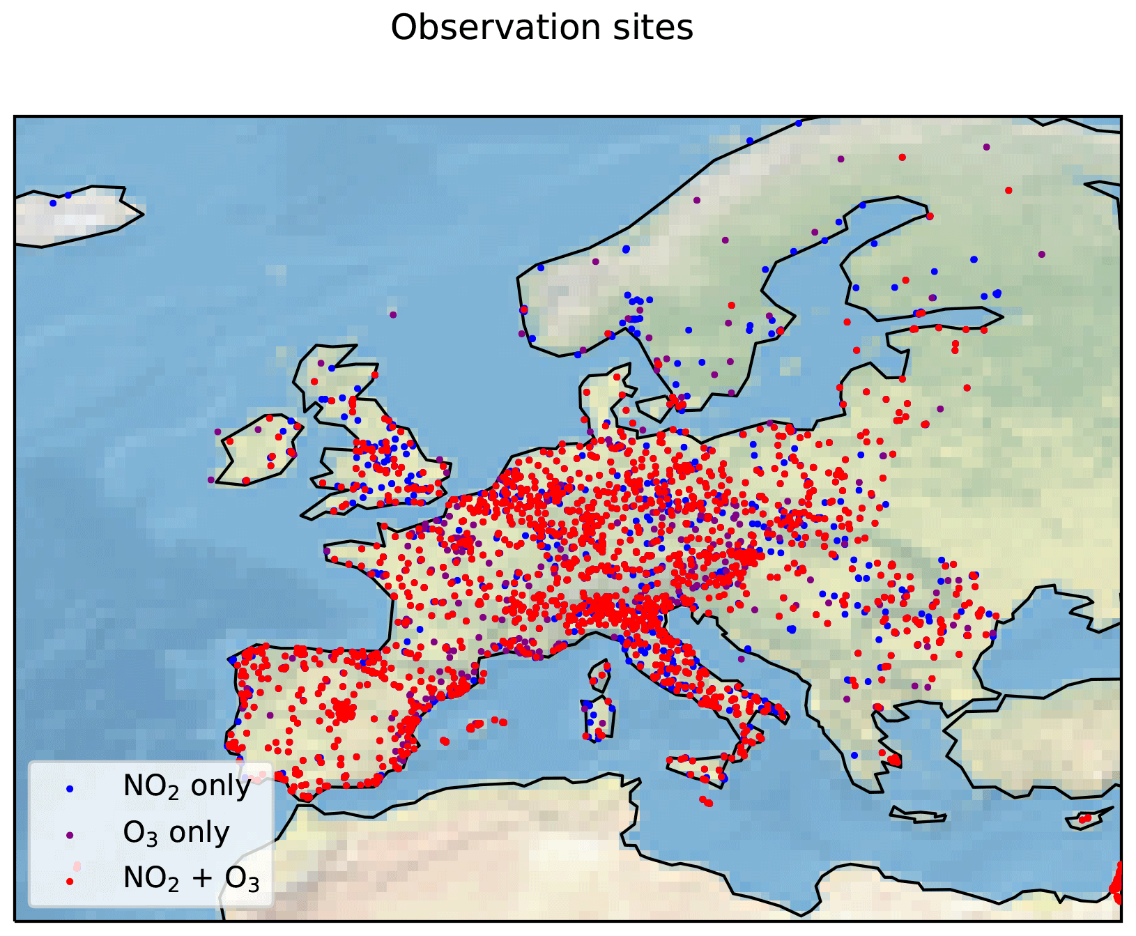
Figure A2Close-up image of European observation sites included in the analysis. Red points indicate sites with both NO2 and O3 observations, purple points show locations with O3 observations only, and blue points show locations with NO2 observations only.
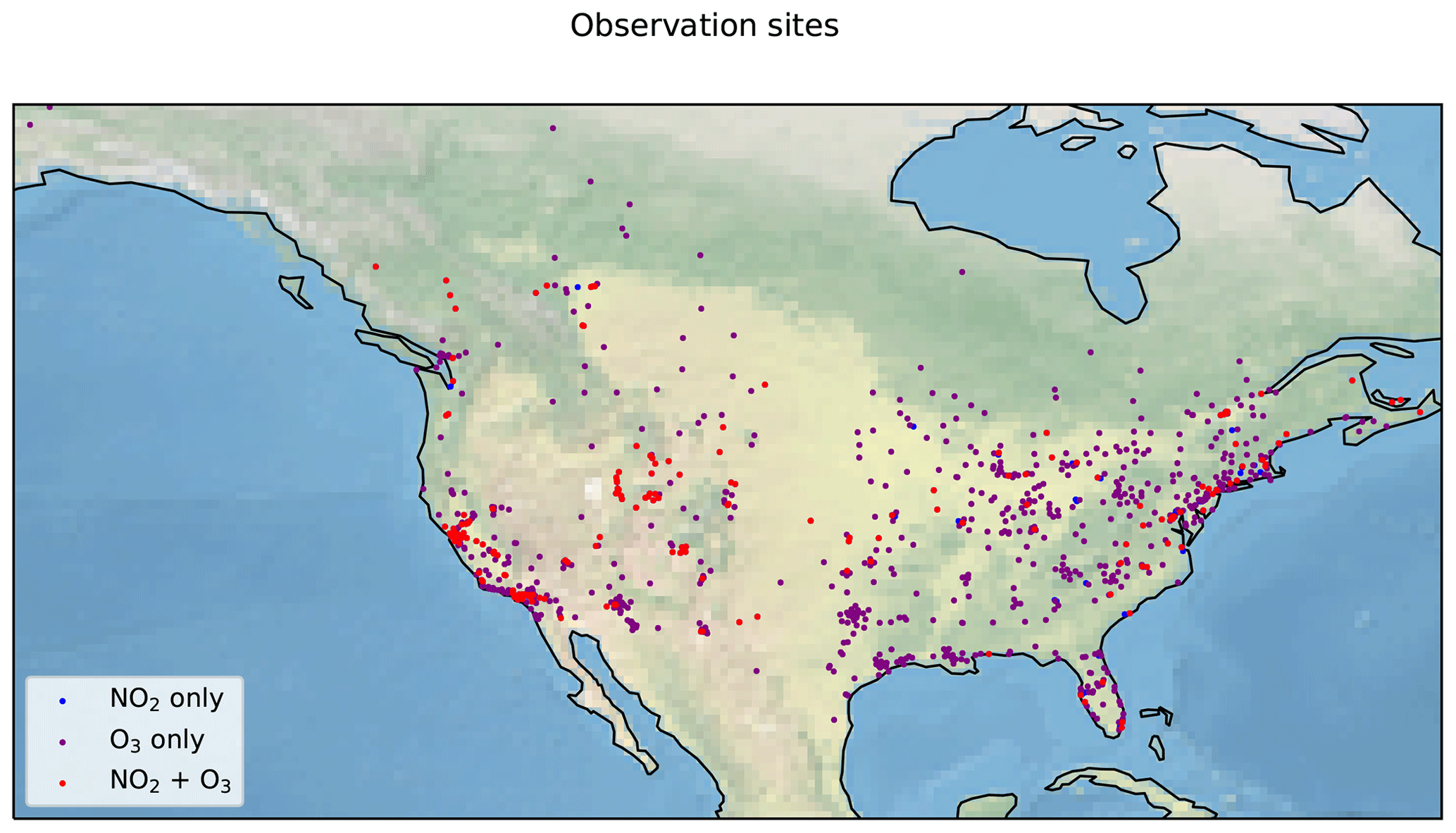
Figure A3Close-up image of North American observation sites included in the analysis. Red points indicate sites with both NO2 and O3 observations, purple points show locations with O3 observations only, and blue points show locations with NO2 observations only.
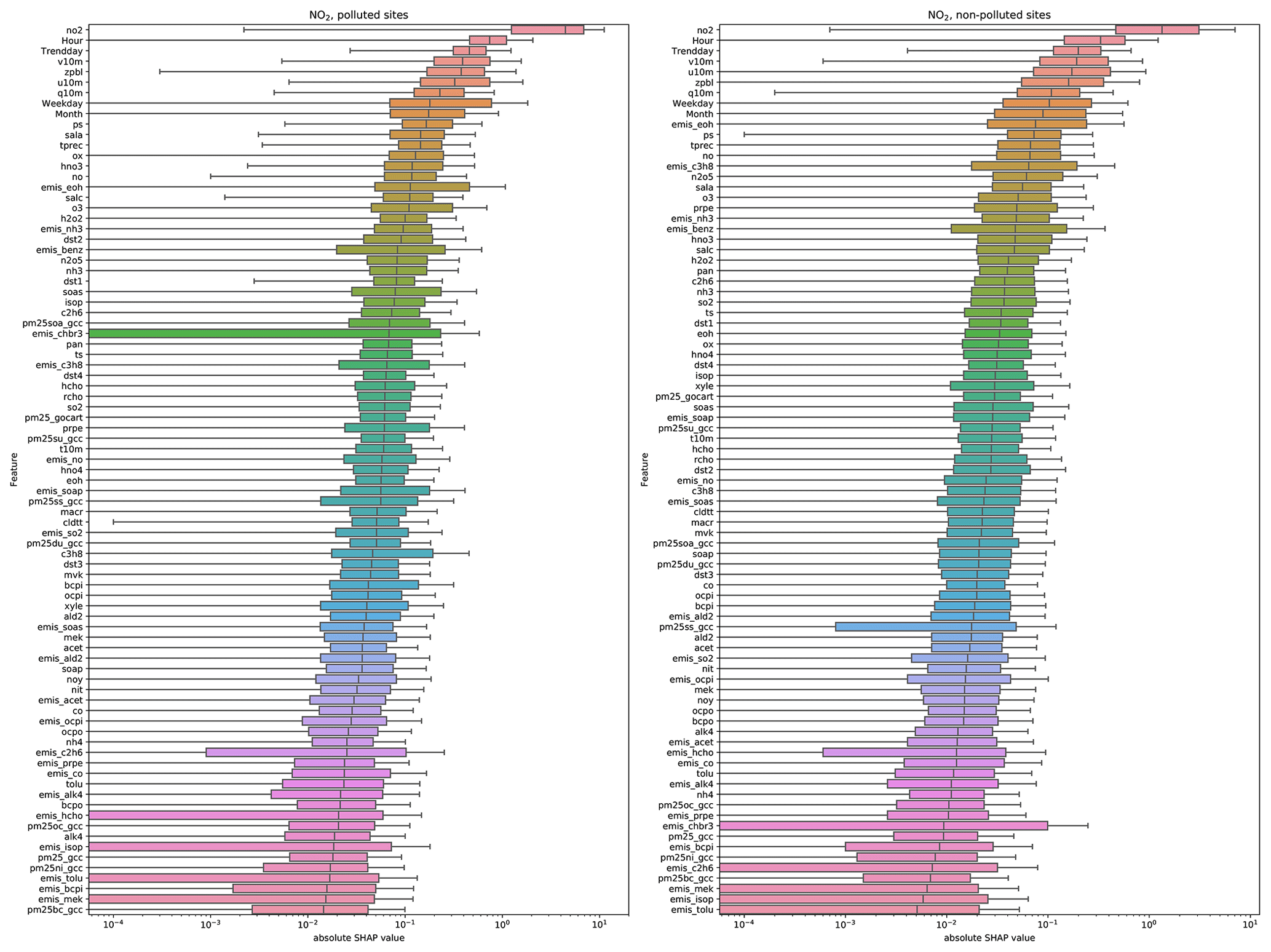
Figure A4Importance of input variables (features) for the XGBoost models trained to predict NO2 model bias. Shown are the distribution of the absolute SHAP values for each feature, ranked by the average importance of each feature. Higher SHAP value indicates higher feature importance. The left panel shows results for polluted sites (average annual NO2 concentration >15 ppbv) and the right panel shows results for all other sites.

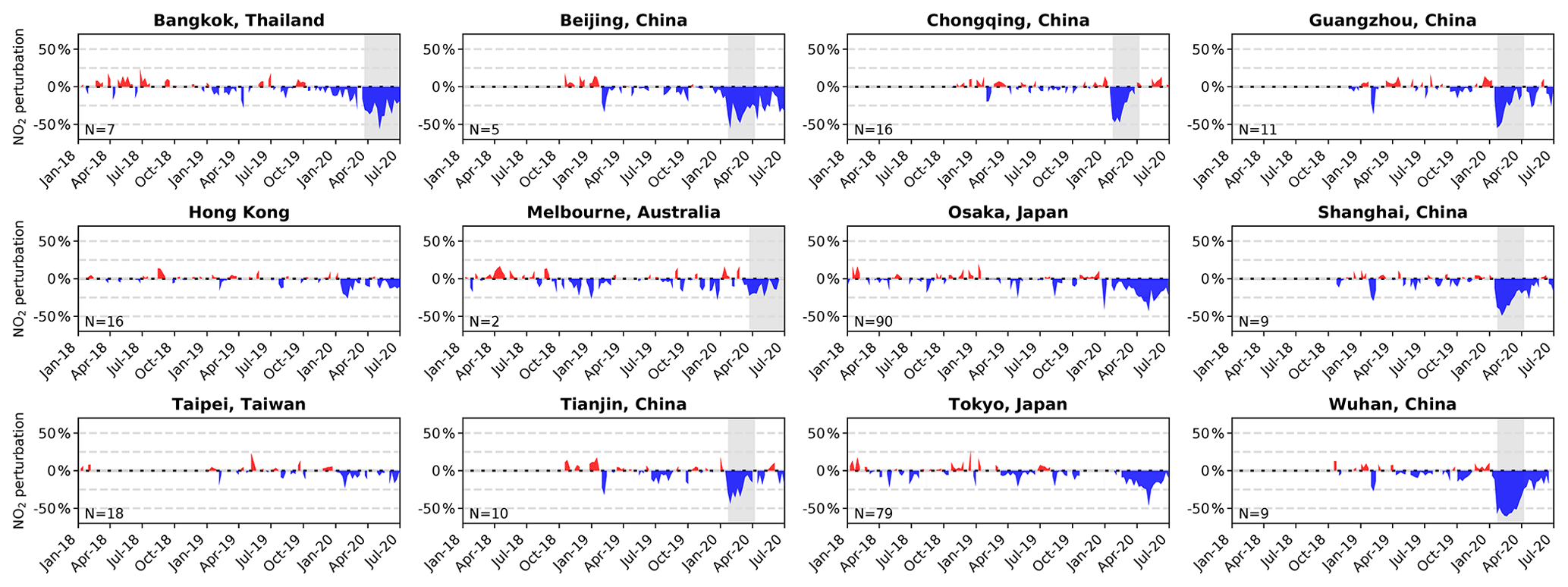
Figure A6Normalized fractional NO2 perturbations (observation–bias-corrected model, normalized by the bias-corrected model prediction) from 1 January 2018 through June 2020 for selected cities in Asia and Australia. Grey-shaded areas indicate COVID-19 lockdown periods. Number of sites per city are shown in the bottom left of each panel.
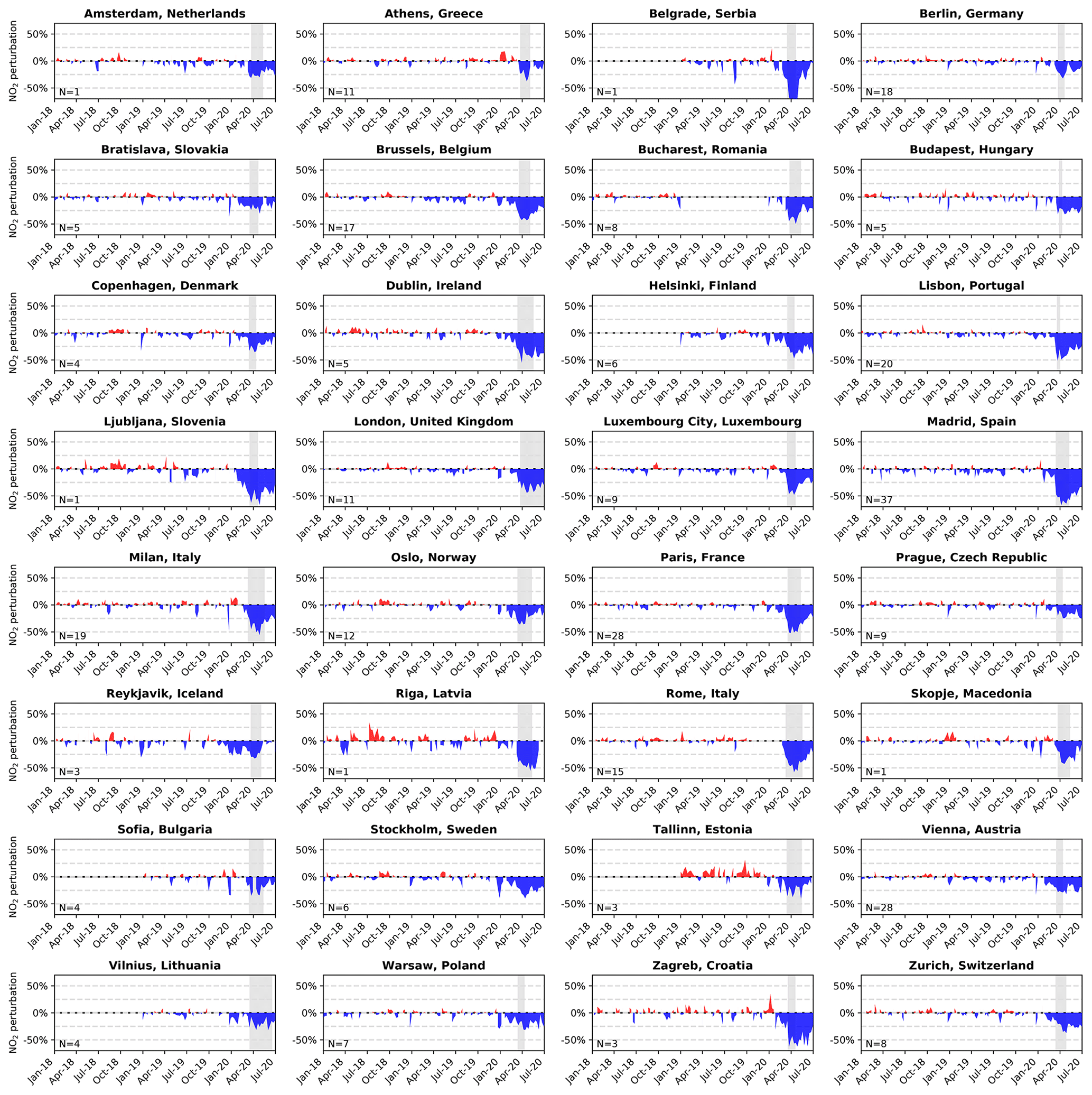
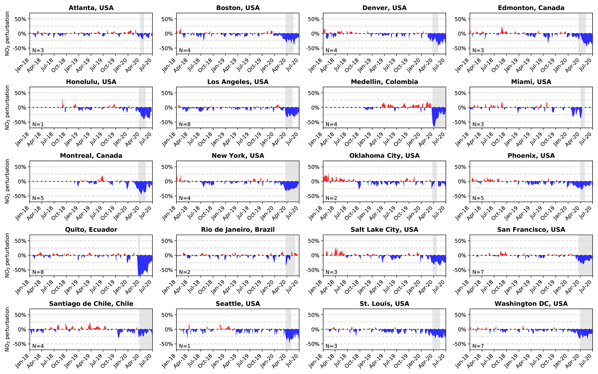
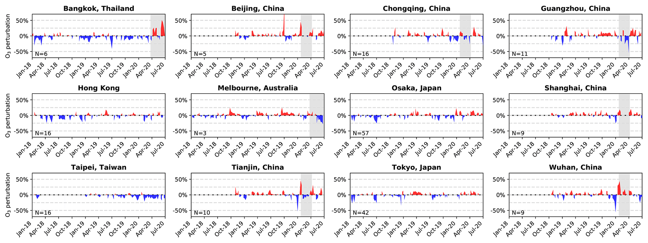
Figure A9Normalized fractional O3 perturbations (observation–bias-corrected model, normalized by the bias-corrected model prediction) from 1 January 2018 through June 2020 for selected cities in Asia and Australia. Grey-shaded areas indicate COVID-19 lockdown periods. Number of sites per city are shown in the bottom left of each panel.
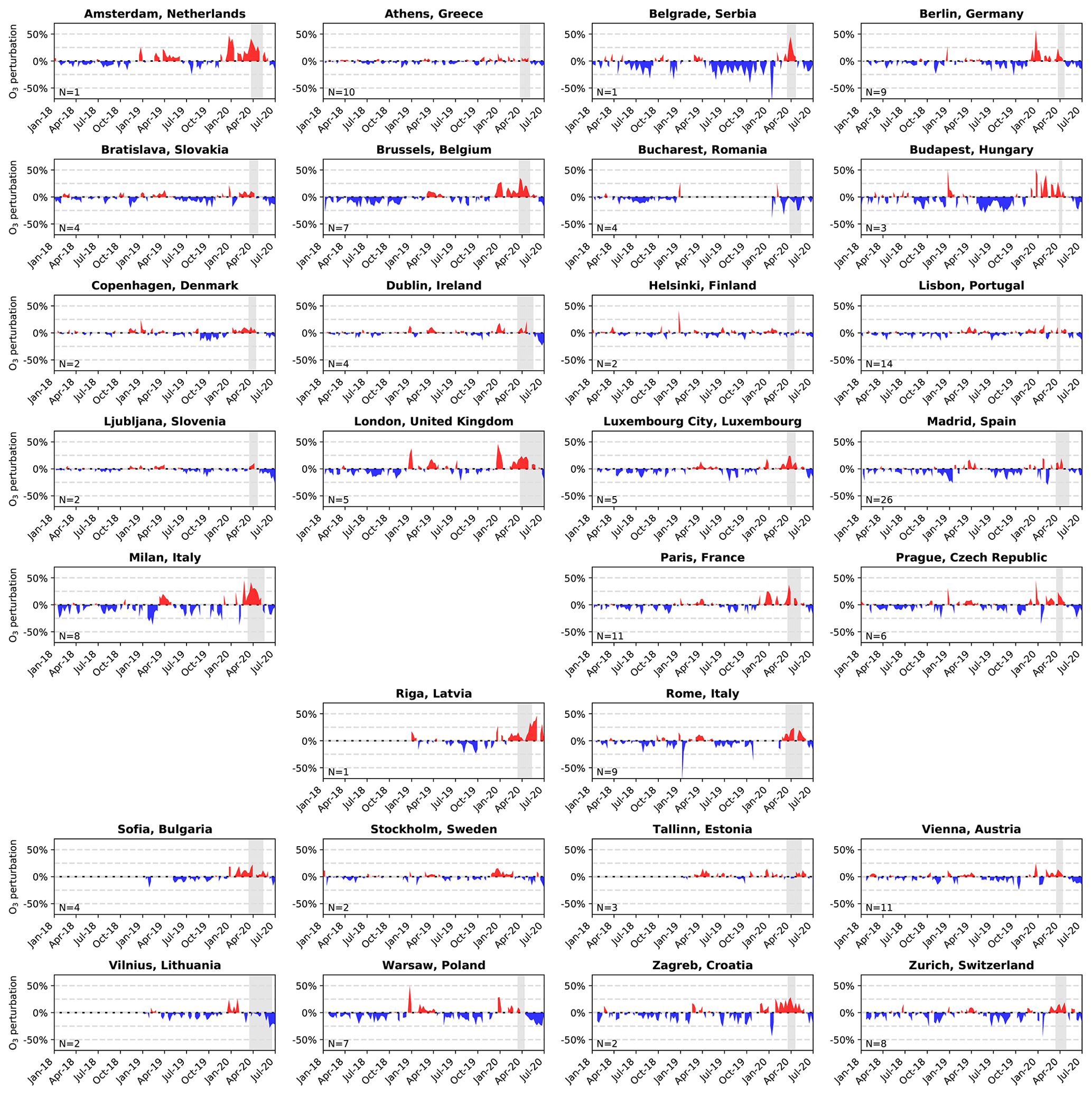
Figure A10The same as Fig. A9 but for Europe. No observations are available for Reykjavik, Oslo, and Skopje.
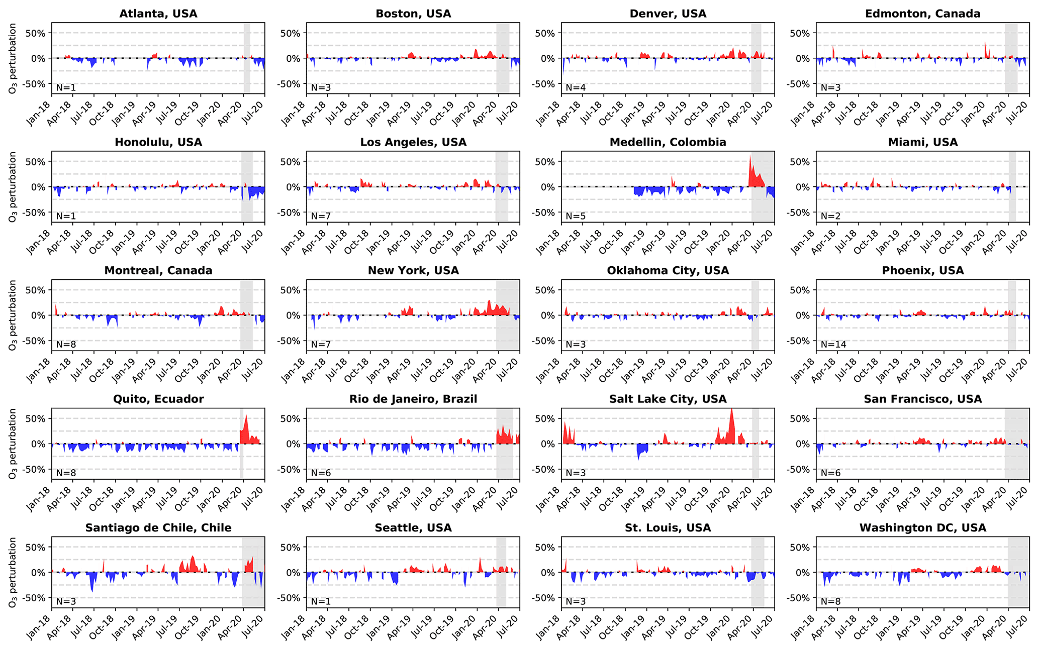
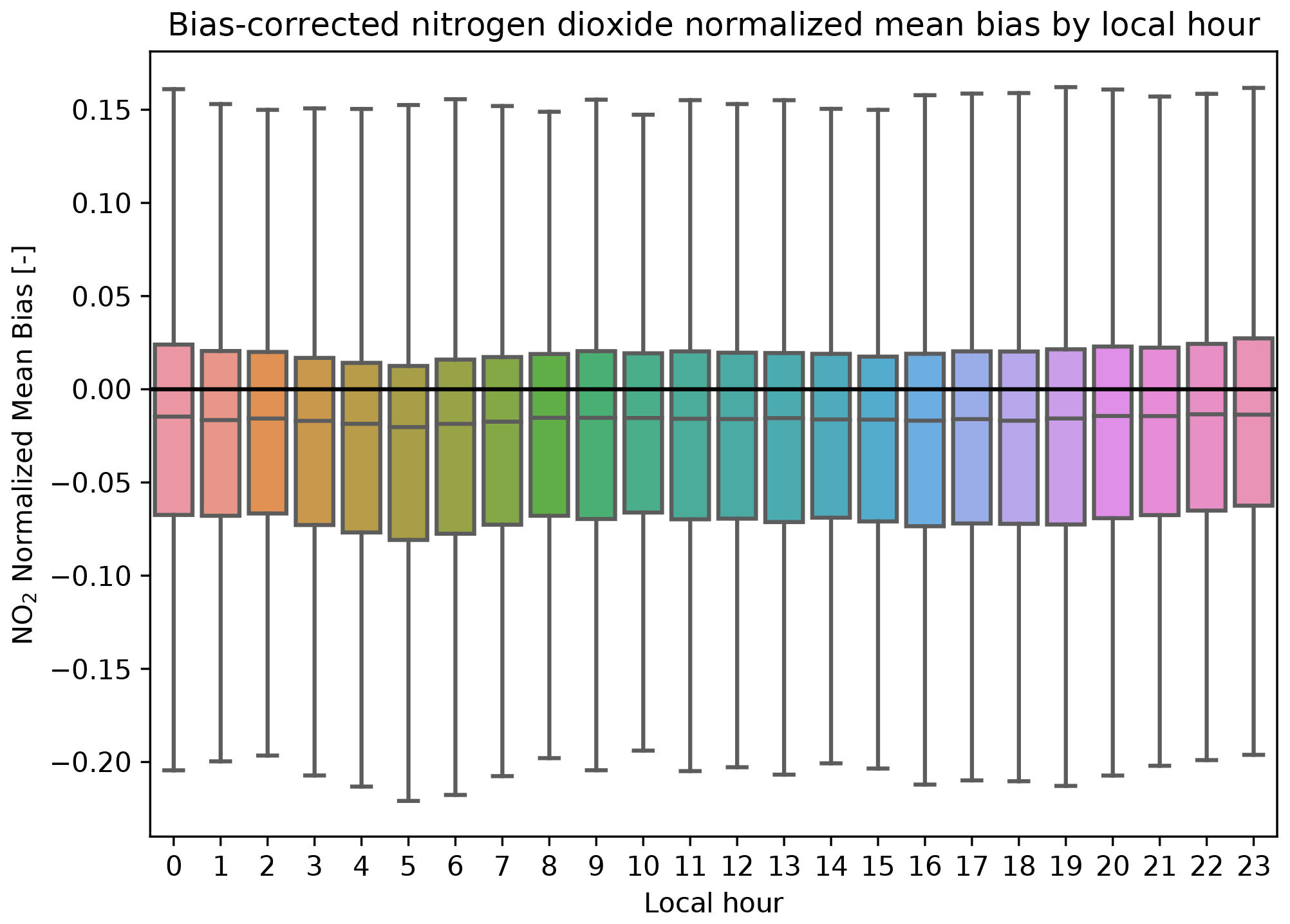
Figure A12Distribution of normalized mean bias of the machine-learning-corrected nitrogen dioxide concentrations at all available observation sites as a function of local hour. Shown are the results for the test dataset.
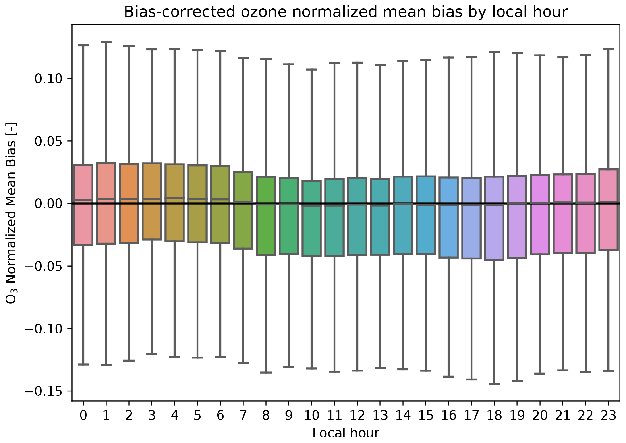
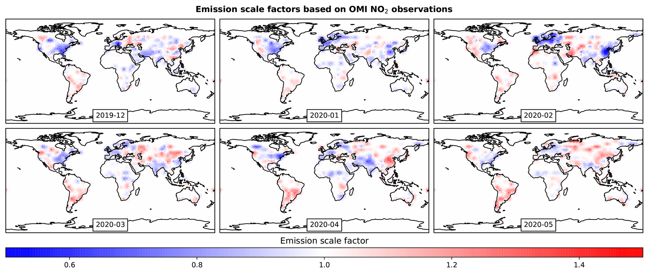
Figure A14Emission scale factors used for model sensitivity simulation. Shown are the monthly average perturbations applied to the GEOS-CF anthropogenic base emissions.
The model output and air quality observations used in this study are all publicly available (see methods). The output from the GEOS-CF sensitivity simulation, as well as the bias-corrected model predictions, are available from Christoph A. Keller upon request.
CAK and MJE designed the study and conducted the main analyses. CAH and SM contributed OpenAQ observations. TO provided observations and interpretations for Japan. FCM and BBF provided observations and interpretations for Rio de Janeiro, and MVDS provided observations and interpretations for Quito. RGR provided observations for Melbourne and helped analyze results for Australia. KEK and RAL conducted the GEOS-CF simulations. KEK and CAK conducted the GEOS-CF sensitivity experiments and forecasts. LHF conducted NOx to NO2 sensitivity simulations. SP contributed to overall study design and context discussion. All authors contributed to the writing.
The authors declare that they have no conflict of interest.
Resources supporting the model simulations were provided by the NASA Center for Climate Simulation at the Goddard Space Flight Center (https://www.nccs.nasa.gov/services/discover, last access: 7 July 2020). We thank Jenny Fisher (University of Wollongong, Australia) for helpful discussions. Mathew J. Evans and Luke H. Fakes are thankful for support from the University of York's Viking HPC facility.
This research has been supported by the NASA Modeling, Analysis and Prediction (MAP) Program (16-MAP16-0025).
This paper was edited by Andreas Richter and reviewed by two anonymous referees.
Boersma, K. F., Eskes, H. J., Dirksen, R. J., van der A, R. J., Veefkind, J. P., Stammes, P., Huijnen, V., Kleipool, Q. L., Sneep, M., Claas, J., Leitão, J., Richter, A., Zhou, Y., and Brunner, D.: An improved tropospheric NO2 column retrieval algorithm for the Ozone Monitoring Instrument, Atmos. Meas. Tech., 4, 1905–1928, https://doi.org/10.5194/amt-4-1905-2011, 2011.
Castellanos, P. and Boersma, K.: Reductions in nitrogen oxides over Europe driven by environmental policy and economic recession, Sci. Rep., 2, 265, https://doi.org/10.1038/srep00265, 2012.
Chen, T. and Guestrin, C.: XGBoost: A Scalable Tree Boosting System, Proceedings of the 22nd ACM SIGKDD International Conference on Knowledge Discovery and Data Mining, August 2016, San Francisco California USA, 785–794, https://doi.org/10.1145/2939672.2939785, 2016.
Crippa, M., Solazzo, E., Huang, G., Guizzardi, D., Koffi, E., Muntean, M., Schieberle, C., Friedrich, R., and Janssens-Maenhout, G.: High resolution temporal profiles in the Emissions Database for Global Atmospheric Research, Sci. Data, 7, 121, https://doi.org/10.1038/s41597-020-0462-2, 2020.
Crippa, M., Guizzardi, D., Muntean, M., Schaaf, E., Dentener, F., van Aardenne, J. A., Monni, S., Doering, U., Olivier, J. G. J., Pagliari, V., and Janssens-Maenhout, G.: Gridded emissions of air pollutants for the period 1970–2012 within EDGAR v4.3.2, Earth Syst. Sci. Data, 10, 1987–2013, https://doi.org/10.5194/essd-10-1987-2018, 2018.
Dantas, G., Siciliano, B., França, B. B., da Silva, C. M., and Arbilla, G.: The impact of COVID-19 partial lockdown on the air quality of the city of Rio de Janeiro, Brazil, Sci. Total Environ., 729, 139085, https://doi.org/10.1016/j.scitotenv.2020.139085, 2020.
Darmenov, A. S. and da Silva, A.: The Quick Fire Emissions Dataset (QFED)–Documentation of versions 2.1, 2.2 and 2.4, Technical Report Series on Global Modeling and Data Assimilation, NASA//TM-2015-104606, Vol. 38, 212 pp., 2015.
Duncan, B. N., Lamsal, L. N., Thompson, A. M., Yoshida, Y., Lu, Z., Streets, D. G., Hurwitz, M. M., and Pickering, K. E.: A space-based, high-resolution view of notable changes in urban NOx pollution around the world (2005–2014), J. Geophys. Res. 121, 976–996, https://doi.org/10.1002/2015JD024121, 2016.
Frery J., Habrard A., Sebban M., Caelen O., and He-Guelton, L.: Efficient Top Rank Optimization with Gradient Boosting for Supervised Anomaly Detection, in: Machine Learning and Knowledge Discovery in Databases, edited by: Ceci, M., Hollmén, J., Todorovski, L., Vens, C., and Džeroski, S., ECML PKDD 2017, Lecture Notes in Computer Science, Vol. 10534, Springer, Cham, https://doi.org/10.1007/978-3-319-71249-9_2, 2017.
Friedman, J. H.: Greedy function approximation: A gradient boosting machine, Ann. Stat., 29, 1189–1232, https://doi.org/10.1214/aos/1013203451, 2001.
Grange, S. K. and Carslaw, D. C.: Using meteorological normalisation to detect interventions in air quality time series, Sci. Total Environ., 653, 578–588, https://doi.org/10.1016/j.scitotenv.2018.10.344, 2019.
Grange, S. K., Carslaw, D. C., Lewis, A. C., Boleti, E., and Hueglin, C.: Random forest meteorological normalisation models for Swiss PM10 trend analysis, Atmos. Chem. Phys., 18, 6223–6239, https://doi.org/10.5194/acp-18-6223-2018, 2018.
Hilboll, A., Richter, A., and Burrows, J. P.: Long-term changes of tropospheric NO2 over megacities derived from multiple satellite instruments, Atmos. Chem. Phys., 13, 4145–4169, https://doi.org/10.5194/acp-13-4145-2013, 2013.
Hu, L., Keller, C. A., Long, M. S., Sherwen, T., Auer, B., Da Silva, A., Nielsen, J. E., Pawson, S., Thompson, M. A., Trayanov, A. L., Travis, K. R., Grange, S. K., Evans, M. J., and Jacob, D. J.: Global simulation of tropospheric chemistry at 12.5 km resolution: performance and evaluation of the GEOS-Chem chemical module (v10-1) within the NASA GEOS Earth system model (GEOS-5 ESM), Geosci. Model Dev., 11, 4603–4620, https://doi.org/10.5194/gmd-11-4603-2018, 2018.
Ivatt, P. D. and Evans, M. J.: Improving the prediction of an atmospheric chemistry transport model using gradient-boosted regression trees, Atmos. Chem. Phys., 20, 8063–8082, https://doi.org/10.5194/acp-20-8063-2020, 2020.
Janssens-Maenhout, G., Crippa, M., Guizzardi, D., Dentener, F., Muntean, M., Pouliot, G., Keating, T., Zhang, Q., Kurokawa, J., Wankmüller, R., Denier van der Gon, H., Kuenen, J. J. P., Klimont, Z., Frost, G., Darras, S., Koffi, B., and Li, M.: HTAP_v2.2: a mosaic of regional and global emission grid maps for 2008 and 2010 to study hemispheric transport of air pollution, Atmos. Chem. Phys., 15, 11411–11432, https://doi.org/10.5194/acp-15-11411-2015, 2015.
Jhun, I., Coull, B. A., Zanobetti, A., and Koutrakis, P.: The impact of nitrogen oxides concentration decreases on ozone trends in the USA, Air Qual. Atmos. Health., 8, 283–292, https://https://doi.org/10.1007/s11869-014-0279-2, 2015.
Keller, C. A., Long, M. S., Yantosca, R. M., Da Silva, A. M., Pawson, S., and Jacob, D. J.: HEMCO v1.0: a versatile, ESMF-compliant component for calculating emissions in atmospheric models, Geosci. Model Dev., 7, 1409–1417, https://doi.org/10.5194/gmd-7-1409-2014, 2014.
Keller, C. A., Knowland, K. E., Duncan, B. N., Liu, J., Anderson, D. C., Das, S., Lucchesi, R. A., Lundgren, E. W., Nicely, J. M., Nielsen, J. E., Ott, L. E., Saunders, E., Strode, S. A., Wales, P. A., Jacob, D. J., and Pawson, S.: Description of the NASA GEOS Composition Forecast Modeling System GEOS-CF v1.0, Earth and Space Science Open Archive, p. 38, https://doi.org/10.1002/essoar.10505287.1, 2020.
Kleinert, F., Leufen, L. H., and Schultz, M. G.: IntelliO3-ts v1.0: a neural network approach to predict near-surface ozone concentrations in Germany, Geosci. Model Dev., 14, 1–25, https://doi.org/10.5194/gmd-14-1-2021, 2021.
Knowland, K. E., Keller, C. A., and Lucchesi, R.: File Specification for GEOS-CF Products, GMAO Office Note No. 17 (Version 1.1), 37 pp., available at: http://gmao.gsfc.nasa.gov/pubs/office_notes, last access: 4 July 2020.
Lamsal, L. N., Martin, R. V., Padmanabhan, A., van Donkelaar, A., Zhang, Q., Sioris, C. E., Chance, K., Kurosu, T. P., and Newchurch, M. J.: Application of satellite observations for timely updates to global anthropogenic NOx emission inventories, Geophys. Res. Lett., 38, L05810, https://https://doi.org/10.1029/2010GL046476, 2011.
Le, T., Wang, Y., Liu, L., Yang, J., Yung, Y. L., Li, G., and Seinfeld, J. H.: Unexpected air pollution with marked emission reductions during the COVID-19 outbreak in China, Science, 702–706, https://https://doi.org/10.1126/science.abb7431, 2020.
Le Quéré, C., Jackson, R. B., Jones, M. W., Smith, A. J. P., Abernethy, S., Andrew, R. M., De-Gol, A. J., Willis, D. R., Shan, Y., Canadell, J. G., Friedlingstein, P., Creutzig, F., and Peters, G. P.: Temporary reduction in daily global CO2 emissions during the COVID-19 forced confinement, Nat. Clim. Change, 647–653, https://doi.org/10.1038/s41558-020-0797-x, 2020.
Liu F., Page, A., Strode, S. A., Yoshida, Y., Choi, S., Zheng, B., Lamsal, L. N., Li, C., Krotov, N. A., Eskes, H., van der A., R., Veefkind, P., Levelt, P. F., Hauser, O. P., and Joiner, J.: Abrupt decline in tropospheric nitrogen dioxide over China after the outbreak of COVID-19, Sci. Adv., 6, 28, https://doi.org/10.1126/sciadv.abc2992, 2020a.
Liu, Z., Ciais, P., Deng, Z., Lei, R., Davis, S. J., Feng, S., Zheng, B., Cui, D., Dou, X., Zhu, B., Guo, R., Ke, P., Sun, T., Lu, C., He, P., Wang, Y., Yue, X., Wang, Y., Lei, Y., Zhou, H., Cai, Z., Wu, Y., Guo, R., Han, T., Xue, J., Boucher, O., Boucher, E., Chevallier, F., Tanaka, K., Wei, Y., Zhong, H., Kang, C., Zhang, N., Chen, B., Xi, F., Liu, M., Breon, F-M., Lu, Y., Zhang, Q., Guan, D., Gong, P., Kammen, D. M., He, K., and Schnellhuber, H. J.: Near-real-time monitoring of global CO2 emissions reveals the effects of the COVID-19 pandemic, Nat. Commun., 11, 5172, https://doi.org/10.1038/s41467-020-18922-7, 2020b.
Long, M. S., Yantosca, R., Nielsen, J. E., Keller, C. A., da Silva, A., Sulprizio, M. P., Pawson, S., and Jacob, D. J.: Development of a grid-independent GEOS-Chem chemical transport model (v9-02) as an atmospheric chemistry module for Earth system models, Geosci. Model Dev., 8, 595–602, https://doi.org/10.5194/gmd-8-595-2015, 2015.
Lucchesi, R.: File Specification for GEOS-5 FP-IT, GMAO Office Note No. 2 (Version 1.4) 58 pp., available at: http://gmao.gsfc.nasa.gov/pubs/office_notes.php (last access: 4 July 2020), 2015.
Lundberg, S. M. and Lee, S.-I.: A unified approach to interpreting model predictions, Adv. Neural Inf. Process. Syst., 30, 4768–4777, 2017.
Lundberg, S. M., Erion, G., Chen, H., DeGrave, A., Prutkin, J. M., Nair, B., Katz, R., Himmelfarb, J., Bansal, N., and Lee, S.-I.: From local explanations to global understanding with explainable AI for trees, Nat. Mach. Intell., 2, 56–67, https://doi.org/10.1038/s42256-019-0138-9, 2020.
Ministry of the Environment (MOE), Government of Japan: The Atmospheric Environmental Regional Observation System (AEROS), available at: http://soramame.taiki.go.jp/Index.php last access: 3 July 2020 (in Japanese).
Petetin, H., Bowdalo, D., Soret, A., Guevara, M., Jorba, O., Serradell, K., and Pérez García-Pando, C.: Meteorology-normalized impact of the COVID-19 lockdown upon NO2 pollution in Spain, Atmos. Chem. Phys., 20, 11119–11141, https://doi.org/10.5194/acp-20-11119-2020, 2020.
Russell, A. R., Valin, L. C., and Cohen, R. C.: Trends in OMI NO2 observations over the United States: effects of emission control technology and the economic recession, Atmos. Chem. Phys., 12, 12197–12209, https://doi.org/10.5194/acp-12-12197-2012, 2012.
Shah, V., Jacob, D. J., Li, K., Silvern, R. F., Zhai, S., Liu, M., Lin, J., and Zhang, Q.: Effect of changing NOx lifetime on the seasonality and long-term trends of satellite-observed tropospheric NO2 columns over China, Atmos. Chem. Phys., 20, 1483–1495, https://doi.org/10.5194/acp-20-1483-2020, 2020.
Seinfeld, J. H. and Pandis, S. N.: Atmospheric Chemistry and Physics: From Air Pollution to Climate Change, John Wiley & Sons, Hoboken, 2016.
Streets, D. G., Canty, T., Carmichael, G. R., de Foy, B., Dickerson, R. R, Duncan, B. N., Edwards, D. P., Haynes, J. A., Henze, D. K., Houyoux, M. R., Jacob, D. J., Krotkov, N. A., Lamsal, L. N., Liu, Y., Lu, Z., Martin, R. V., Pfister, G. G., Pinder, R. W., Salawitch, R. J., and Wecht, K. J.: Emissions estimation from satellite retrievals: A review of current capability, Atmos. Environ., 77, 1011–1042, https://doi.org/10.1016/j.atmosenv.2013.05.051, 2013.
Tobías, A., Carnerero, C., Reche, C., Massagué, J., Via, M., Minguillón, M. C., Alastuey, A., and Querol, X.: Changes in air quality during the lockdown in Barcelona (Spain) one month into the SARS-CoV-2 epidemic, Sci. Total Environ., 726, 138540, https://doi.org/10.1016/j.scitotenv.2020.138540, 2020.
Wargan, K., Pawson, S., Olsen, M. A., Witte, J. C., Douglass, A. R., Ziemke, J. R., Strahan, S. E., and Nielsen, J. E.: The Global Structure of Upper Troposphere-Lower Stratosphere Ozone in GEOS-5: A Multi-Year Assimilation of EOS Aura Data, J. Geophys. Res.-Atmos, 120, 2013–2036, https://https://doi.org/10.1002/2014JD022493, 2015.