the Creative Commons Attribution 4.0 License.
the Creative Commons Attribution 4.0 License.
 | 09 Mar 2021
The impact of inhomogeneous emissions and topography on ozone photochemistry in the vicinity of Hong Kong Island
Yong-Feng Ma
Domingo Muñoz-Esparza
Cathy W. Y. Li
Mary Barth
Guy P. Brasseur
Global and regional chemical transport models of the atmosphere are based on the assumption that chemical species are completely mixed within each model grid box. However, in reality, these species are often segregated due to localized sources and the influence of topography. In order to investigate the degree to which the rates of chemical reactions between two reactive species are reduced due to the possible segregation of species within the convective boundary layer, we perform large-eddy simulations (LESs) in the mountainous region of Hong Kong Island. We adopt a simple chemical scheme with 15 primary and secondary chemical species, including ozone and its precursors. We calculate the segregation intensity due to inhomogeneity in the surface emissions of primary pollutants and due to turbulent motions related to topography. We show that the inhomogeneity in the emissions increases the segregation intensity by a factor of 2–5 relative to a case in which the emissions are assumed to be uniformly distributed. Topography has an important effect on the segregation locally, but this influence is relatively limited when considering the spatial domain as a whole. In the particular setting of our model, segregation reduces the ozone formation by 8 %–12 % compared to the case with complete mixing, implying that the coarse-resolution models may overestimate the surface ozone when ignoring the segregation effect.
- Article
(8364 KB) - Full-text XML
- BibTeX
- EndNote


The spatial distribution of reactive species in the atmosphere derived by global or regional chemical–meteorological models is obtained by solving a system of nonlinear continuity (mass conservation) equations coupled with the Navier–Stokes (momentum) and energy conservation equations (Brasseur and Jacob, 2017). In most cases, a numerical approximation of the solution of these partial differential equations is found at a finite number of locations on a grid that covers the three-dimensional (3D) geographical domain under consideration. The size of the spatial patterns that is explicitly resolved by such models is determined by the size of the adopted grid meshes. Smaller features, called subgrid-scale (SGS) processes, which influence the large-scale dynamical and chemical solutions, are often represented by closure relations based on empirical parameterizations.
With the computer resources currently available, the spatial resolution adopted for the discretization of the model equations is typically of the order of 50–100 km in the case of global models and 1–50 km in the case of regional models used for operational numerical weather and climate predictions. Thus, in both cases, small-scale processes such as turbulent motions in the boundary layer, mountain flows, sea breeze, urban dynamics, and shallow clouds, as well as the complexity of surface chemical emissions, are crudely represented or parameterized. Coarse models, for example, assume total mixing between trace species inside each grid mesh and therefore do not accurately account for the segregation that may exist between these species in turbulent flows. The segregation effect is important for fast reactions, of which the chemical timescale is shorter than the turbulent timescale. In this case the reactants remain segregated rather than reacting, and such segregation tends to reduce the averaged rate at which chemical reactions happen within a model grid mesh (Komori et al., 1991; Schumann, 1989). Previous studies, such as Vilà-Guerau de Arellano and Duynkerke (1993) and Kramm and Meixner (2000), considered the segregation effect in the boundary layer parameterization in the chemical transport models and showed that it is important to take the segregation into account in current photochemical models.
Numerical treatment of the turbulent flow can be provided by large-eddy simulation (LES) models. LES is a rapidly evolving approach for modeling the turbulent flows, which was initially proposed by Smagorinsky (1963) and first explored by Deardorff (1970). In this approach, the unsteady Navier–Stokes and continuity equations are filtered to remove the smallest eddies while capturing the eddy motions at a size larger than a specified cutoff width. The interactions of the larger, resolved eddies and the smaller, unresolved eddies are addressed by specifying a SGS stress model (Deardorff, 1970; Smagorinsky, 1963).
The LES technique has been used in past studies to quantify the segregation effect in the turbulent atmospheric boundary layer. Schumann (1989) simulated a single reaction in the convective boundary layer with one bottom-up and one top-down tracer and showed that the segregation of one reaction is dependent on the ratio of the chemical and turbulent timescales, the concentration ratio of the two reactants, and the initial condition. Patton et al. (2001) used LES to simulate scalars that are emitted from forest canopy with different decay rates and presented the influence of chemical reactivity on the scalar distribution, variance, and vertical flux, which affect the segregation. Other LES studies with different configurations of surface emissions pointed out that spatially inhomogeneous emissions influence the segregation intensities considerably. These studies, such as Krol et al. (2000), Auger and Legras (2007), and Ouwersloot et al. (2011), mainly focused on isoprene chemistry and compared the segregation intensities of the reaction between isoprene and the hydroxyl radical (OH) with homogenous and inhomogeneous isoprene emissions and showed that the heterogeneity in the emissions largely increases the segregation intensities. There are other factors that affect the segregation intensities. For example, Li et al. (2016) investigated the sensitivity of the segregation of volatile organic compounds (VOCs) to weather conditions (e.g., temperature, humidity, and the presence of clouds). They showed that isoprene segregation is largest under warm and convective conditions. Kim et al. (2016) showed that the segregation intensity of isoprene and OH differs at low- and high-nitrogen-oxide (NOx) levels caused by the primary production and loss reactions of OH under a different NOx regime. Li et al. (2017) added the effect of aqueous-phase chemistry in a LES model and showed that the segregation of OH and isoprene is enhanced in clouds. Studies focusing on isoprene chemistry in a forested region have been initiated to understand the underestimation of the OH in global models (Dlugi et al., 2019; Ouwersloot et al., 2011). These studies all used flat domains and calculated the domain-averaged segregation intensities to account for the errors induced by the turbulence in regional or global models. However, the impact of the terrain on the segregation was not considered. Previous studies showed that complex terrain has an important impact on the turbulence structure in the boundary layer (e.g., Cao et al., 2012; Rotach et al., 2015; Liang et al., 2020) and on the evolution with time of the boundary layer height (De Wekker and Kossmann, 2015). Therefore, the segregation intensity is expected to be affected by the topography.
This paper uses a LES model included in the Weather Research and Forecasting (WRF) model (Skamarock et al., 2008, 2019) to investigate the importance of segregation between reacting species in an area where surface emissions are spatially very inhomogeneous and the flow is turbulent under the influence of a complex topography. Under such conditions, the vertical mixing and the reaction rates between chemical species in the boundary layer are expected to be sensitive to the strength of the large eddies. The simulations are performed in a geographical area covering Hong Kong Island. The surface wind measurements from the Hong Kong Observatory (HKO) station show the prevailing wind blowing from the east about 80 % of the time and from the west about 15 % of the time (Shu et al., 2015). There are two important features in the air pollution in Hong Kong: the pollution sources are concentrated in the very dense urban region, mostly along the coast, while natural emissions occur in large forested areas in the center of the island; both regions are separated by complex topography. With the intense and inhomogeneous emissions in such an urban environment, the resultant segregation can cause a large impact on the calculation of chemical reactions (Li et al., 2021). This impact is expected to be even larger with the influence of complex topography. In this study, we therefore set up a domain with a mountainous terrain characterized by complex flows determined by the topography and the occurrence of related turbulent motions.
The purpose of the study is to investigate the importance of interactions between chemistry and turbulence in the planetary boundary layer (PBL) as well as to assess how the spatial segregation between chemical species affects the nonlinear production and destruction rates of key chemical species including ozone. Since the study is intended to be conceptual, we adopt a simple chemical scheme to represent the chemical interactions between ozone and its precursors. We make plausible assumptions about the spatial distribution of the surface emissions of primary species emitted in the forested and urbanized areas of the island. We estimate how the vertical eddy transport fluxes of the chemical species and the covariance between their concentrations, generally unaccounted for in coarse atmospheric models, affect the distribution of chemical species in the lowest levels of the atmosphere in the vicinity of the island.
The present modeling study should be viewed as a step towards a more complex and realistic investigation of chemical and turbulent processes occurring in the densely populated urban area of Hong Kong, characterized by a complex urban canopy of high-rise buildings and street canyons built on an uneven topography surrounded by the ocean and affected by emissions in mainland China and other Asian countries and by the presence of an active harbor with intense shipping in the region. The present study focuses on the impact of the heterogenous emissions and the turbulent flow generated by the topography on chemical processes. The model description and dynamical and chemical settings are introduced in Sect. 2. Results of the large-eddy simulations and the interpretations of the model output are presented in Sect. 3. Section 4 provides the principal conclusions of this study.
2.1 Model description
The WRF model (version 4.0.2) with the ARW (Advanced Research WRF) core (Skamarock et al., 2008, 2019) was used to perform mesoscale meteorology simulations that provided the initial fields for the large-eddy simulations. The LES module included in WRF was run in an idealized mode as implemented and evaluated by Moeng et al. (2007), Kirkil et al. (2012), and Yamaguchi and Feingold (2012). A low-pass filter was applied to separate the large and small eddies, where the large eddies (energy-injection scales near the classic inertial range of 3D turbulence) were explicitly resolved, while the small eddies were parameterized by the SGS model. In the idealized LES, the initial physical conditions were specified by uniform values over the entire domain; a random perturbation was imposed initially on the mean temperature field at the lowest four grid levels to initiate the turbulent motions.
2.2 Dynamical settings
A nested two-domain setup was adopted for the LES simulation. The size of the outer domain was 45 km × 45 km, and the spatial resolution was 300 m. The size of the inner domain was 24 km × 24 km, with a horizontal grid spacing of 100 m. The vertical layers were the same for both domains with 100 vertical levels, and the model top was set at 4 km altitude. Double periodic boundary conditions were used in both the west–east and south–north directions for the outer domain. One-way nesting was used, in which the outer domain provided turbulence-inclusive boundary conditions for the inner domain (Moeng et al., 2007; Muñoz-Esparza et al., 2014).
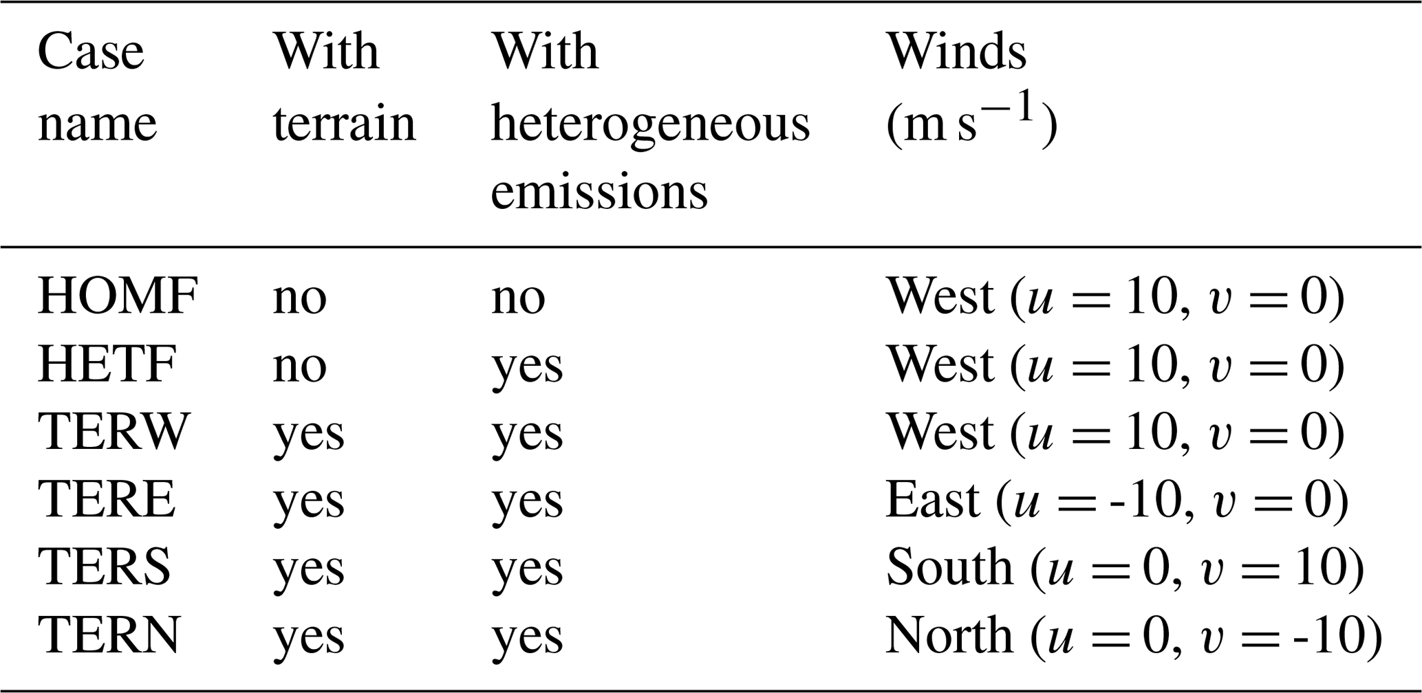
The initial profiles for the potential temperature (θ) and water mixing ratio (q) for the outer domain were taken from the output of the mesoscale WRF run operated at a spatial resolution of 1.33 km (shown by the dashed green line in Fig. 1) and were interpolated to 40 m vertical grid spacing, with the highest level located at 4 km. The date (1 August 2018) and time of the day (04:00 UTC; 12:00 local time) were chosen to correspond to a typical summer condition in Hong Kong with a well-developed convective boundary layer. Four cases were considered, with initial winds blowing uniformly from the west (TERW; TER stands for terrain), the east (TERE), the south (TERS), and the north (TERN), respectively. The initial wind speed in each case was equal to 10 m s−1.
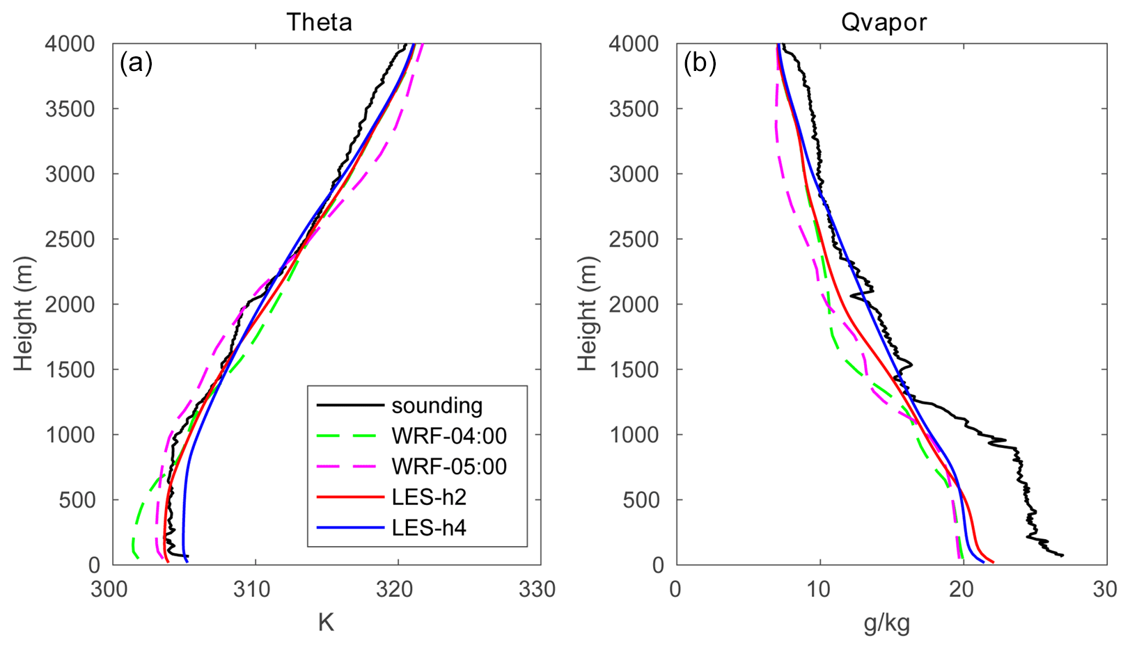
Figure 1The evolution of the profiles for potential temperature (a) and water mixing ratio (b) from mesoscale WRF (dashed green lines at 04:00 UTC; dashed magenta lines at 05:00 UTC) and LES (solid red lines for hour 2 from the start time; solid blue lines for hour 4). The measurements at King's Park station taken at 05:00 UTC are shown by black lines (data source: http://www.hko.gov.hk, last access: 13 January 2020).
The LES version adopted here used Deardorff's turbulent kinetic energy (TKE) scheme to compute the SGS eddy viscosity and eddy diffusivity for turbulent mixing. The Coriolis parameter was set according to the latitude of Hong Kong Island. The Kessler microphysics scheme (Kessler, 1969) was used to derive cloudiness in the model. The WRF's radiation, land surface, and PBL schemes were all turned off. We applied a fixed sensible heat flux of 230 W m−2 at the bottom boundary, while the latent heat flux was calculated in the model from the surface water vapor content specified at the beginning of the simulations. We chose to apply a relatively small sensible heat flux (compared to summer noon conditions in Hong Kong) in order to produce a gradual development of the boundary layer and keep the convection condition unchanged during the course of the simulation. With this choice, the buoyancy flux was dominated in the simulation by the kinematic sensible heat flux, which is about 2–3 times larger than the kinematic moisture heat flux.
The outer model domain was assumed to be entirely flat, while the inner domain included a representation of the topography of Hong Kong Island. This modeling setup followed the approach of Kosović et al. (2014). The elevation of the surface was taken from the ALOS world 3D data (Takaku et al., 2014), distributed by OpenTopography (https://opentopography.org; last access: 1 June 2020), with a spatial resolution of 30 m. To avoid numerical errors due to the terrain-following coordinate, the terrain was somewhat smoothed in areas where the surface slope exceeds 25∘. The smoothed terrain height is shown in Fig. 2a. To simplify the simulation, and to focus on the terrain shape instead of the terrain types, the surface of the entire domain was set as land to ignore the influence of the sea.
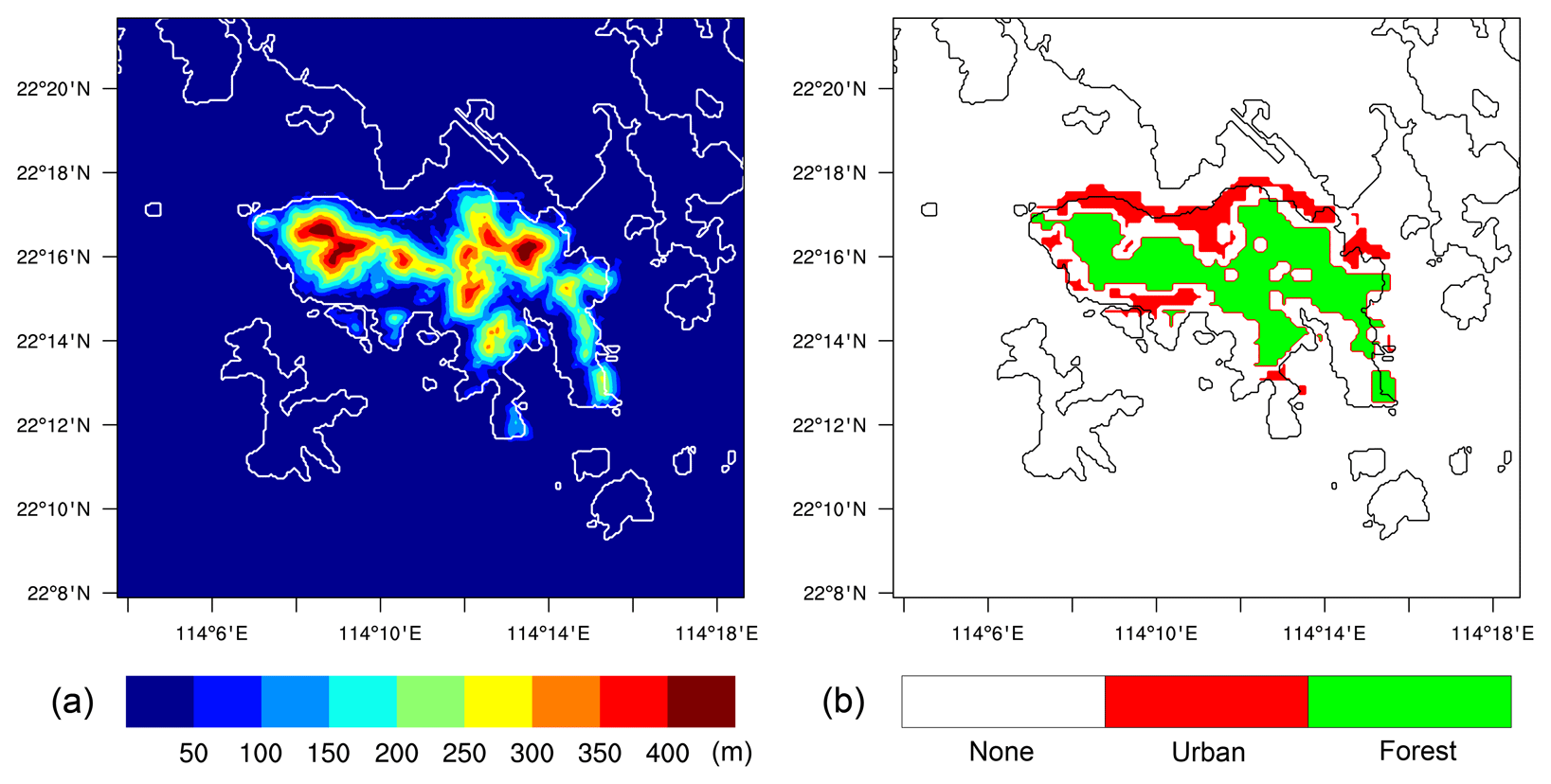
Figure 2Elevation of the topography for Hong Kong Island (a) and emission map (b); red is the anthropogenic emission area, and green represents the biogenic emission.
2.3 Chemical settings
A simple O3–NOx–VOC chemical mechanism with 15 reactive species and 18 photochemical reactions (see Table 1) was adopted in this conceptual study and is based on the simple scheme for ozone production from hydrocarbon oxidation described in the textbook by Brasseur and Jacob (2017). We included two primary hydrocarbons, RH-A and RH-B, which represent anthropogenic (labeled -A) and biogenic (labeled -B) VOCs, respectively. RH-A was treated as a surrogate for propane and RH-B as a surrogate for isoprene. The corresponding rate constants (k) for the oxidation by the hydroxyl radical OH at a temperature of 300 K are equal to 1.1 × 10⁻¹² and 1.0 × 10⁻¹⁰ cm3 molec.−1 s−1, respectively. We can derive the lifetime of RH-A and RH-B by the expression , with the respective values of the rate constants k. With an OH concentration ([OH]) of 5 × 10⁶ molec. cm−3, the corresponding chemical lifetimes of RH-A and RH-B are approximately 2 d and 30 min, respectively.
Table 1The chemical reactions used in the model. The unit of first-order reaction rate coefficients is per second (s−1) and that of second-order reaction rate coefficients is cubic centimeters per molecule per second (cm3 molec.−1 s−1).
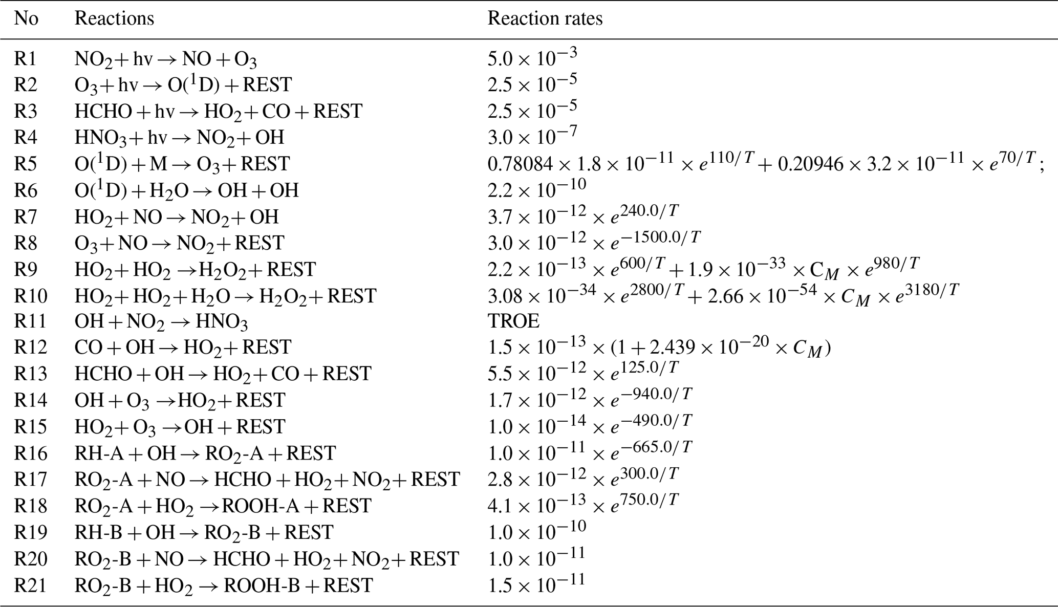
Note that T stands for temperature, M stands for air, CM stands for the air density, and REST stands for the products that are not evaluated. TROE = × 0.6, k1= 2.6 × 10−30 × (300)3.2 × CM, k2= )1.3).
Among all the species, NO, CO, RH-A, and RH-B were emitted at the surface. The background conditions of the polluted atmosphere were represented by assuming emission rates in the outer domain to be uniform, with values of 1.2 × 10¹², 8.0 × 10¹², and 7.0 × 10¹¹ molec. cm−2 s−1, for NO, CO, and RH-A respectively. The RH-B emission was set to be 3.0 × 10¹¹ molec. cm−2 s−1 for the conditions in Hong Kong with a large tropical forested area. For the inner domain, we considered two specific regions corresponding to urban and forested areas, based on information provided by the land use map from ESA CCI (ESA, 2017; https://www.esa-landcover-cci.org, last access: 1 June 2020). The resulting emission map on the nested domain that includes terrain features is shown in Fig. 2b, with NO, CO, and RH-A emitted in the urban region and RH-B emitted in the forested region. The emission rates in the inner domain were calculated by dividing the corresponding values adopted in the outer domain by the area fraction of the corresponding land use type, so that the averaged emission rates for the whole inner domain were the same as those of the outer domain. In order to separate the influence of the emissions and topography, two additional simulations were conducted. A simulation with homogeneous emissions and without topography for both domains (HOMF; HOM stands for homogeneous emission; F stands for flat terrain) was performed as a baseline experiment. To assess the role of the inhomogeneous emissions in our results, a simulation with flat terrain but with inhomogeneous emissions as shown in Fig. 2b (referred to as HETF; HET stands for heterogeneous emission; F stands for flat terrain) was also conducted. The details of all the experiments are listed in Table 2.
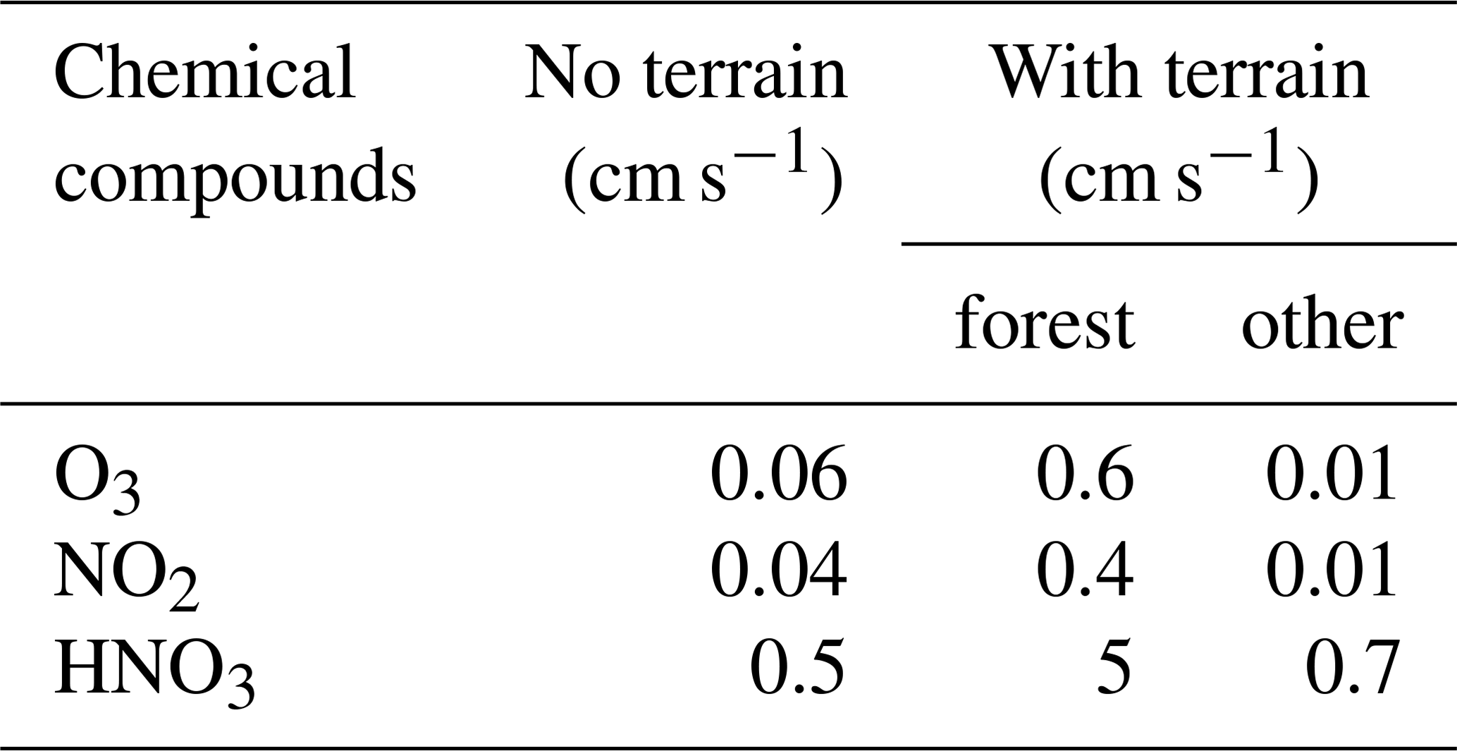
An atmospheric destruction of reservoir species (HNO3, H2O2, ROOH-A, ROOH-B) was applied to balance the surface emissions of the primary species. The removal of these reservoirs by photolytic processes in the atmosphere is slow (more than 2 weeks in the case of HNO3 and several days for peroxides), so that most of the loss is due to wet removal or dry deposition. The model did not consider the possible occurrence of convective precipitation as often observed during summertime in Hong Kong, and hence no detailed formulation was used for the wet removal in the LES model. However, in order to keep a balance (stationary state) in the background concentrations and avoid an accumulation of species produced from the ongoing emissions, the removal of the soluble species HNO3, H2O2, ROOH-A, and ROOH-B occurred with a first-order rate of 2.5 × 10⁻⁵ s−1 (lifetime of about half a day). This lifetime may be viewed as representing the mean time period separating successive convective rain events during summertime. For the dry deposition on the surface, for the grass/forested areas outside the urbanized regions we adopted values based on the measurements of Wu et al. (2011) and on the analysis of Ganzeveld and Lelieveld (1995). The values were reduced over urban areas. The detailed deposition velocities for the different species and the different land types are provided in Table 3.
In order to generate reasonable initial profiles for the chemical species for the two-domain simulations and to reduce the spin-up time, a simple one-domain LES simulation was run for 2 d using the same chemical scheme as in the two-domain simulation. The one-domain LES used the same homogeneous emissions as described above. The time-varying photolysis rates were calculated by the TUV (tropospheric ultraviolet and visible) scheme for producing the diurnal variation in the photochemistry. The domain-averaged profiles for the chemical species at 12:00 local time of the second day were then used as the chemical initial profiles for the two-domain simulations. The initial profiles are shown by green lines in Fig. 3.
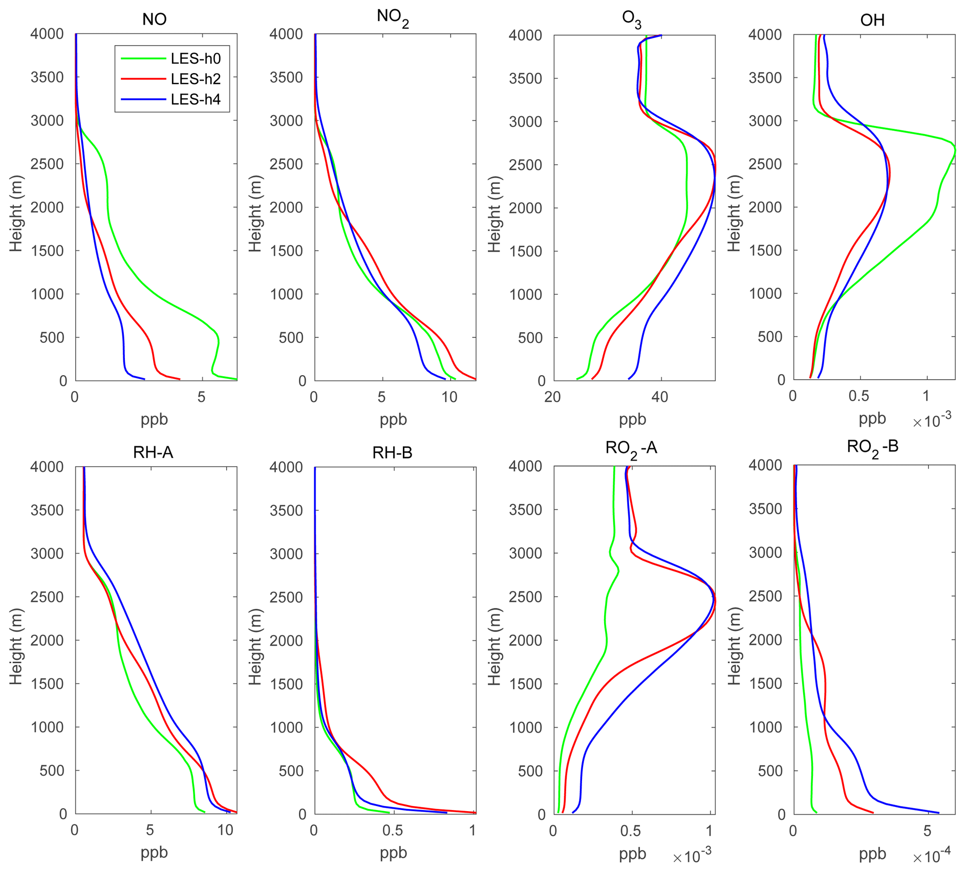
Figure 3Domain-averaged profiles of the selected chemical compounds at the initial time (green lines), hour 2 (red lines), and hour 4 (blue lines) for the HOMF case.
2.4 Formulations of chemistry–turbulence interactions
Following the concept of the Reynolds decomposition, any physical variable A, such as the concentration of chemical species, can be expressed as the sum between its mean value 〈A〉 (here 〈〉 stands for time average) and the fluctuation A′ caused, for example, by turbulent motions:
For a second-order chemical reaction,
with the reaction rate constant,
where k0 and T0 are reaction-dependent constants, and the rate R of the reaction is expressed as
If we ignore the temperature fluctuation (i.e., , the averaged reaction rate is
where is the chemical covariance between the two reacting chemicals, and IAB is called the segregation intensity (Danckwerts, 1952), defined as
The intensity of the segregation is therefore equal to the covariance of the two reactants divided by the product of their mean concentrations. IAB is equal to zero when the chemicals A and B are fully mixed and equal to −100 % when the two chemicals are fully segregated. For initially segregated A and B, the corresponding segregation intensity is closer to −100 % if the chemical reaction between the two species is fast. IAB is positive when the concentrations of the two chemicals are correlated.
The intensity of segregation between two species A and B is related to the Damköhler number (Da) (Damköhler, 1940):
where τturb is the turbulent timescale (typically 10 min during daytime, considerably longer during nighttime), and τchem, A(B) is the reaction timescale of A when reacting with B. If the chemical timescale of A is shorter than the turbulent timescale (Da > 1; called the fast chemistry limit), the reaction between A and B is limited by the rate at which turbulent motions bring reacting species together; the covariance between fluctuating components as well as the segregation intensity are high. This occurs when the reaction rate constant k is large (Schumann, 1989; Vinuesa and Vilà-Guerau de Arellano, 2005, 2011) or when the emission of A or B is intense (Molemaker and Vilà-Guerau de Arellano, 1998; Kim et al., 2016; Li et al., 2021). Other factors such as inhomogeneous emissions (Ouwersloot et al., 2011; Auger and Legras, 2007; Li et al., 2021) and other structures that obscure mixing also result in a more negative segregation intensity. Under this situation, coarse models such as regional chemical transport models may not provide accurate results since they ignore the influence of subgrid-scale turbulence on the rate at which a reaction between A and B occurs. When the Damköhler number Da≪1 (called the slow chemistry limit), the chemical species A under consideration is well mixed with small covariances with reactant B and with no significant segregation. In this case, the reaction is controlled by chemistry, and its rate is proportional to the product of the mean concentrations. This represents a case in which the rate of chemical reactions is well represented in coarse models. When the Damköhler number is close to 1, the interaction between chemistry and turbulence is strong as the chemical species are equally controlled by chemistry and turbulence.
In the Reynolds decomposition described here, the reaction rate is thus expressed by the sum of two terms: the first term is proportional to the product of the mean concentrations, represented, for example, by the concentration averaged over a grid cell in a global and regional model. The second term accounts for the contribution of subgrid chemical–turbulent interactions and can be estimated using a large-eddy simulation. The effective rate constant keff of a reaction affected by turbulent motions is therefore (Vinuesa and Vilà-Guerau De Arellano, 2005)
Thus, a negative value of the segregation intensity IAB tends to reduce the average rate at which a reaction occurs, while a positive value of IAB leads to an enhancement in this rate.
The segregation intensity can also be written as a function of the correlation coefficient and the concentration fluctuation intensity, as shown in the paper by Ouwersloot et al. (2011). The standard deviation of A is expressed as , and the covariance of A and B is , so the segregation intensity becomes
where
is the correlation coefficient of A and B, which determines the sign of the segregation intensity, while
defined as the concentration fluctuation intensity of A and B, controls the strength of the segregation. In this paper, the mean fields of the chemical species were all calculated as a 1 h time average at given points in the domain.
The simulations for the inner domain were analyzed and are shown in this section. The results of the simulations are presented in several subsections. First, we derive domain-averaged characteristics of physical and chemical quantities (i.e., temperature, humidity, concentrations of chemical species) from a baseline experiment (HOMF) that ran with uniform surface emissions in the absence of topography. Second, we analyze the effects of inhomogeneous (spatially concentrated) surface emissions (HETF) on the distribution of chemical species and on the spatial segregation between reacting species. Third, we discuss the impact of the topography on the same quantities. Finally, we assess the influence of different mean wind directions on our model results.
3.1 General development
The time evolution of the profiles of the potential temperature and water vapor mixing ratio (averaged over the entire domain) is shown in Fig. 1. The dashed lines represent the output from the mesoscale WRF model at a spatial resolution of 1.33 km. The dashed green lines at 04:00 UTC (12:00 local time) represent the initial profiles adopted for the LES simulation, and the dashed magenta lines are the WRF output at 05:00 UTC (13:00 local time). At this time, the temperature has increased in the boundary layer, and the top of the PBL has been lifted in response to the warming of the surface. The sounding measurements at 05:00 UTC at King's Park station are used to validate the simulated physical quantities (black lines in Fig. 1). The mesoscale WRF model reproduces the potential temperature quite well, while it underestimates the water vapor mixing ratio, especially in the boundary layer. This may be related to a simulated weaker southerly wind, which results in relatively less water vapor transport from the South China Sea. The red and blue solid lines show the large-eddy simulation (HOMF) after 2 and 4 integration hours, respectively. The simulated water vapor from LES is higher than in the mesoscale model, and the agreement with the measurements is improved, especially at high altitudes. The convective boundary layer height is detected by the virtual potential temperature (θv) gradient method, which is defined as the height where (the subscript “s” represents the surface) first exceeds a threshold value (Liu and Liang, 2010). Due to the constant surface heat flux forcing, the PBL height gradually increases with a trend of ∼0.028 m s−1. The PBL height is about 797 and 985 m at hour 2 and hour 4, respectively. This deepening tendency of the PBL is the same as in the mesoscale WRF simulation, but the growth in the PBL height in LES is slower than that in WRF because of the small surface heat flux adopted in the LES model. It should be noted that the derived PBL heights are sensitive to the estimation methods (e.g., Seidel et al., 2010; Li et al., 2019). The virtual potential temperature gradient method is chosen because the calculated PBL height is consistent with that derived in the mesoscale WRF. However, to be considered as realistic, the calculated PBL heights should be compared to a sufficient number of observations rather than mesoscale WRF estimates. In fact, the PBL processes and cloud convection are difficult to be represented in the mesoscale models (Mapes et al., 2004; Barth et al., 2007), and the derived PBL heights are strongly affected by the cloud physics and PBL schemes adopted in the simulations (e.g., Li et al., 2019). The estimated turbulent timescale for the LES simulation is about 9 min, which is similar to timescales reported in previous studies (e.g., Anfossi et al., 2006).
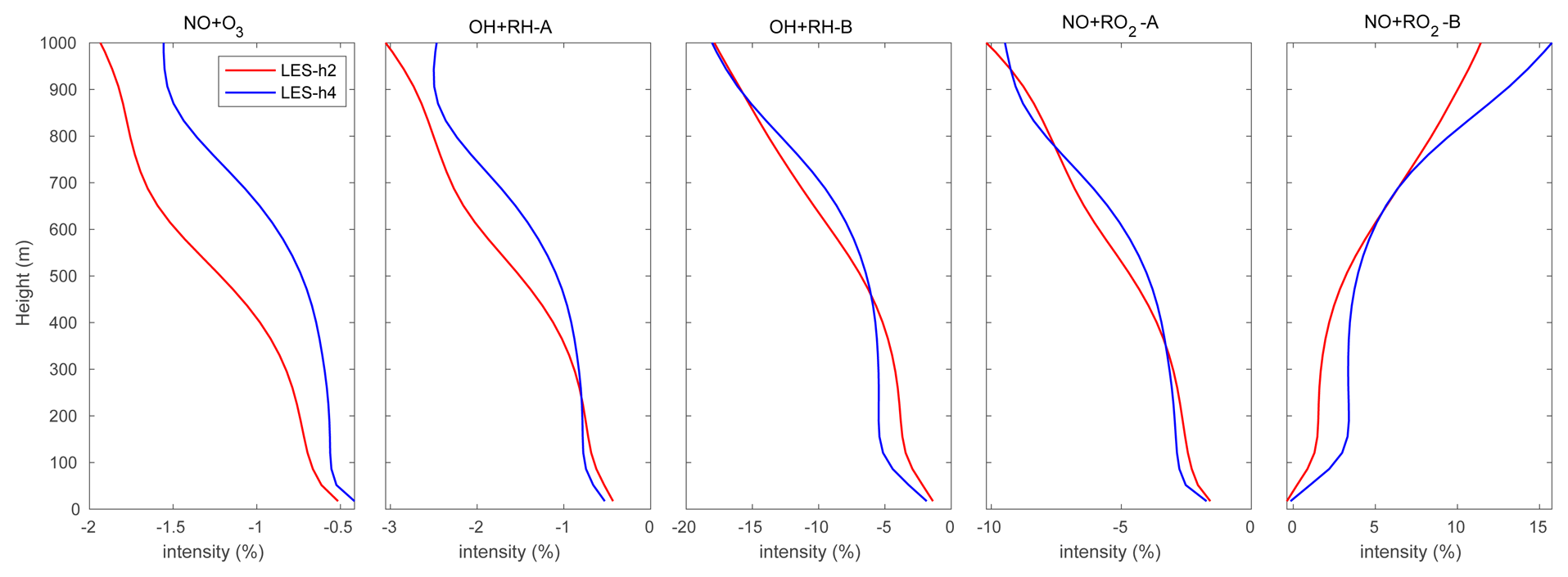
Figure 4Domain-averaged segregation intensity profiles of selected reactions at hour 2 (red) and hour 4 (blue) for the HOMF case.
Figure 3 shows the domain-mean profiles of several chemical species at hours 2 and 4. The green lines represent the initial profiles applied in the LES model. The profiles at hours 2 and 4 are very similar, which suggests that stationary conditions have been reached in the LES simulation. The atmospheric concentrations of the species emitted at the surface (NO, RH-A, RH-B) are largest near the ground and decrease with altitude. Because O3 is consumed by NO and since NO is highest at the surface, the O3 concentration is lowest in the bottom layers of the model. The same situation exists for OH that reacts with the primary species CO, RH-A, and RH-B that are emitted at the surface. NO2 is produced by the reaction between NO and O3; this reaction is therefore largely dependent on the NO concentration, so that the NO2 shows a similar profile to that of NO. RO2-A and RO2-B are produced by the oxidation by OH of RH-A and RH-B; however, RH-A reacts more slowly than RH-B, and therefore the RO2-A vertical profile is more affected by the concentration of OH than RO2-B that shares the same structure as that of RH-B.
In order to assess the average effect of turbulence on the reaction rates, we calculated the segregation intensities (IAB) using Eq. (6) and averaged them over the entire domain (shown in Fig. 4) for the following five reactions:
Among these reactions, Reaction (R8) plays a key role in linking the atmospheric levels of tropospheric ozone and nitrogen oxides; Reactions (R16) and (R17) represent the degradation path of anthropogenic VOCs, while Reactions (R19) and (R20) account for the same reactions but for biogenic VOCs. In this study, we only analyze the segregation effect in the boundary layer up to 800 m to avoid the more complex influence from clouds that are formed higher up in the atmosphere. Using Eq. (7), we derive in the daytime boundary layer Damköhler numbers Da(NO) and Da(O3) of 9.8 and 0.5 respectively for Reaction (R8). The Damköhler numbers for the degradation of primary anthropogenic and biogenic hydrocarbons RH-A and RH-B by the hydroxyl radical OH are 0.004 and 0.3, respectively. This indicates that the oxidation of the anthropogenic hydrocarbon (surrogate of propane) is slow, while it is considerably faster in the case of the biogenic hydrocarbon (surrogate of isoprene). The value of 0.3 calculated for RH-B is in the range of 0.01–1.0 derived by previous studies of isoprene (e.g., Patton et al., 2001; Vinuesa and Vilà-Guerau de Arellano, 2005; Li et al., 2016; Dlugi et al., 2019). The Damköhler numbers for the reaction of peroxy radicals with nitric oxide, Da(RO2-A) and Da(RO2-B), are equal to 188 and 248 respectively, which indicates that the reaction of the organic peroxy radicals with NO is fast for both species from anthropogenic and biogenic origins (Verver et al., 2000). The calculation of the Damköhler number is sensitive to several factors including the weather conditions and the concentration of the species (Li et al., 2016). As a result, the calculated values of Da can vary over a wide range and change as one adopts a different chemical mechanism. The horizontal averaged segregation profiles for the selected reactions from the surface to 1000 m are shown in Fig. 4. For the LES experiment with flat terrain and homogenous emissions, the segregation is weak near the surface and becomes larger at higher altitudes. It is generated by the turbulent patterns of the flow. The segregation intensities for Reactions (R8), (R16), (R17), and (R19) are negative, which highlights the anti-correlation between the atmospheric concentration of the reactants. The segregation intensity, however, is positive in the case of Reaction (R20) because RO2 and NO are positively correlated. We calculated the statistics from the segregation fields for the center region of the domain (14 × 14 km2) so that we exclude the influence of the buffering zone near the lateral boundaries of the domain. We provide values for two altitude layers: 0–500 and 500–800 m, as shown in Table 4. The separation at 500 m is adopted to make comparisons with subsequent simulations in which the effect of the terrain is considered. The mean segregation intensity for the reaction between NO and O3 is −0.60 % below 500 m and −0.95 % above 500 m, which are the smallest values among the five selected reactions. This results from the fact that the reaction rate between NO and O3 is relatively small, as well as the rapid cycling between NO and NO2. The intensities for the reaction between the anthropogenic hydrocarbon (RH-A) and OH are −0.84 % at the lowest levels and −1.52 % at the highest level, respectively. The reaction of the biogenic hydrocarbon (RH-B) is considerably faster than that of RH-A; as a result, segregation is as large as −5.08 % and −8.38 % for the low and high levels, respectively. The calculated segregation intensity for RH-B and OH is comparable to the values from previous studies, e.g., −7 % (PBL-averaged), as reported for the homogeneous case by Ouwersloot et al. (2011), and −5 % to −6 %, as found by Kim et al. (2016). Kim et al. (2016) showed that the segregation intensity between isoprene and OH varies with NOx levels. This results from the fact that the primary OH production and loss rates vary according to the NOx regime under consideration. Therefore, the differences between values reported by different studies can be attributed, at least in part, to the different NOx levels. Ouwersloot et al. (2011) used a low-NOx condition, while our study considers a polluted situation with high-NOx concentrations. In order to further compare with the previous studies, the relationship between segregation intensity and correlation coefficient (r) for the reaction between RH-B and OH is plotted in Fig. 5. The calculated correlation coefficients are mostly in the range of −0.6 to −1.0, which is consistent with the model results from Ouwersloot et al. (2011), while they are larger than the measurements from some campaigns resulting from the measurement noise (Dlugi et al., 2019). The mean values calculated for NO and RO2-A are −3.14 % and −5.38 %. For the reaction of the positively correlated species, NO and RO2-B, the segregation intensities are +2.77 % and +5.43 %.
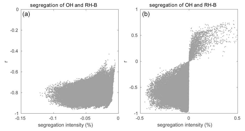
Figure 5Relationship between segregation intensity and correlation coefficient (r) for the reaction between OH and RH-B for (a) the HOMF simulation and (b) the HETF case.
Table 4List of the calculated segregation intensities for the center region (14 × 14 km2) of the domain.
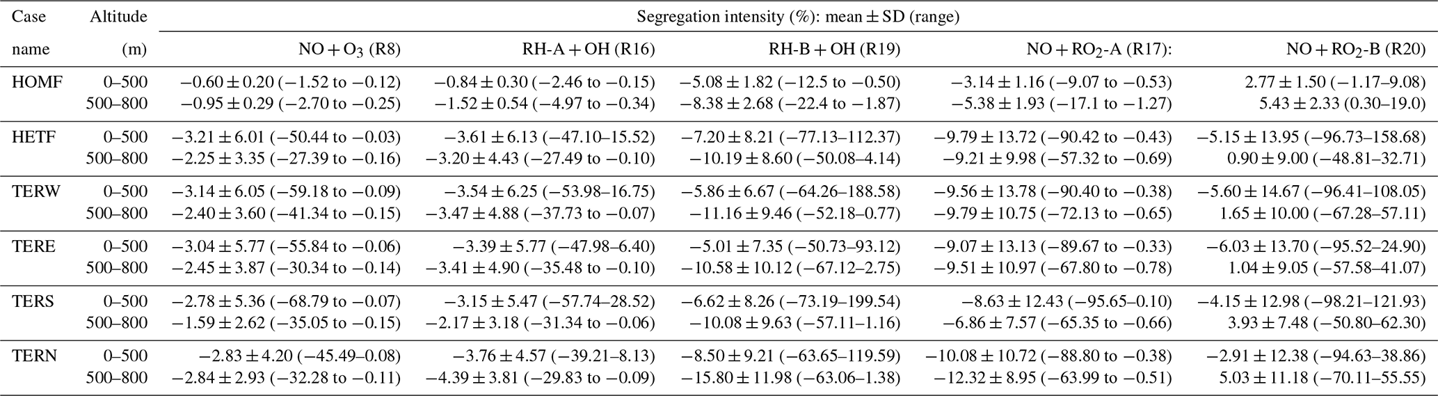
Figure 4 also shows that the negative segregation intensities are larger for hour 2 than for hour 4 of the simulation, while the positive segregation is smaller at hour 2 compared to hour 4. This highlights the enhanced mixing of the tracers as time proceeds, so that the reactions become increasingly effective.
3.2 Impact of inhomogeneous surface emissions on the chemical reactions
To investigate the impact of the spatially inhomogeneous emissions on Hong Kong Island, a control run (HETF) was conducted using the emission distribution shown in Fig. 2. The mean concentrations of several chemical species near the surface and in a vertical cross section along the west-east direction at latitude 22.275∘ N are shown in Fig. 6. NO with anthropogenic emissions has the highest concentrations in the urban area at the edge of Hong Kong Island. RH-A shares the same pattern as NO, so it is not shown here. Since RH-B has a biogenic source located in the forested region of the island, the highest values are found in the center of the island. NO2 produced by the reaction between NO and O3 shows the same pattern as NO, while O3, which is negatively correlated with NO, exhibits the lowest concentration in the urbanized area. OH, which is depleted by both anthropogenic and biogenic species, is characterized by low concentrations above the whole island. Since the anthropogenic emissions including CO and RH-A are considerably larger than the emissions of RH-B, the OH concentrations are lowest in the urbanized area. The OH concentration also shows peak values at the edge between the areas dominated by anthropogenic and biogenic emissions, where the destruction of the radical is smallest. The organic peroxy radicals of anthropogenic and biogenic origin, RO2-A and RO2-B, share the patterns found for OH and RH-B, respectively. This is consistent with the discussion in Sect. 3.1.
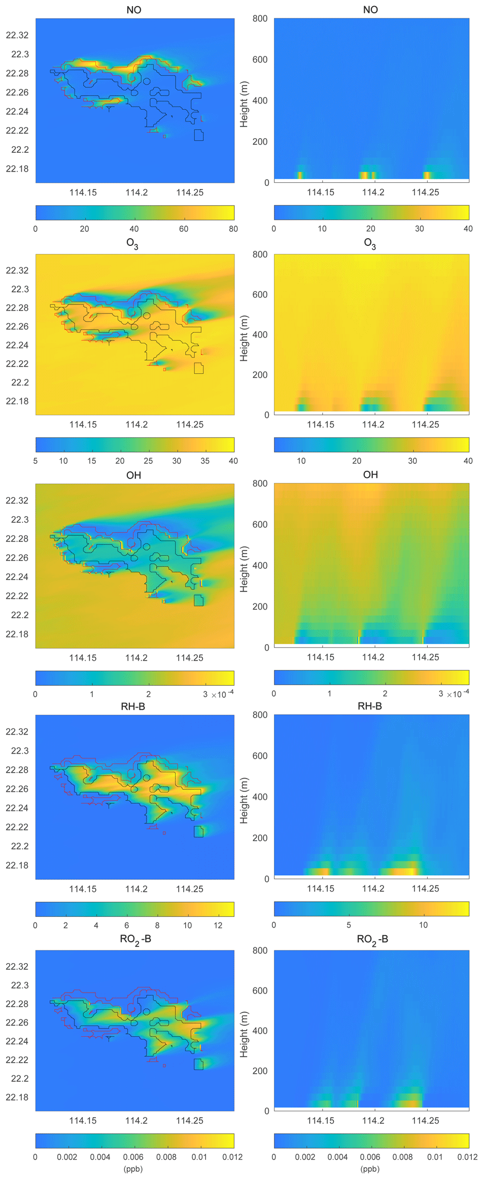
Figure 6Volume mixing ratio of the chemical species at the first level (left panels) and vertical cross section along latitude 22.275∘ N (right panels) at hour 4 for the HETF case. The red line shows the urban area, and the black line shows the forest area.
The segregation intensity derived for the HETF case is shown in Fig. 7. Since the segregation intensities of the reactions of OH with RH-A and NO with RO2-A have similar distribution to that of the NO and O3 reaction, they are not shown in the figure. Different from the HOMF experiment with homogenous emissions, the segregation intensity from the HETF run is largely dependent on the distribution of the emissions. The segregation map near the surface shows that intensity is much larger near the source region than at other locations. For the reaction of NO and O3, the concentration distributions of the two species are opposite to each other, and the segregation effect is negative. Because of the stronger depletion of OH by the anthropogenic species (both CO and RH-A) than by biogenic RH-B, the OH concentration is lower in the urban region and higher in the forest area, which results in a opposite pattern to RH-A. Thus, the segregation effect is negative for the reaction between RH-A and OH. This is also the case for the reaction between NO and RO2-A, since RO2-A follows the pattern of OH. The segregation map for RH-B and OH is complicated, with both positive and negative values, depending on the location; the positive segregation intensities are located mainly at the edge between urban and forested areas, where OH concentration exhibits some peaks in its concentration. Because RH-B depletes OH, the two species are expected to be negatively correlated; however, OH is also consumed by other species, which affects the distributions of the radical. This implies that the heterogenous emissions not only lead to different intensity distributions, but they also can change the sign of the segregation when one chemical species reacts with several species present in different concentrations at separated locations. The correlation coefficient for the RH-B and OH is shown in Fig. 5. Different from the simulation with homogenous emissions, the correlation coefficients vary between −1 and +0.7, which decide the sign of the segregation intensities. From the segregation map near the surface, we can see that the segregation intensities for NO and RO2-B are negative, which is different from the HOMF case in which the emissions are homogeneous. In the HOMF simulation, the emissions of NO and RH-B (which is highly correlated to RO2-B) are co-located, so NO and RO2-B are positively correlated, while in the HETF simulation, the emission of RH-B is separated from the NO emissions, resulting in a negative correlation between NO and RO2-B. The vertical patterns of the segregation intensity, shown in Fig. 7d–f, indicate that the impact of the emission distribution is substantial from the surface to about 500 m height and is affected by the strength of convection. It is seen that the segregation for NO and RO2-B is only negative at low altitudes; it becomes positive at higher levels, where the impact of the separated sources has vanished. This is consistent with what is reported by Ouwersloot et al. (2011) and Li et al. (2021) for their cases with heterogeneous emissions. The large magnitude of segregation intensity between RO2-B and NO near the surface is also comparable to the values reported in Li et al. (2021) in their cases with heterogeneous emissions.
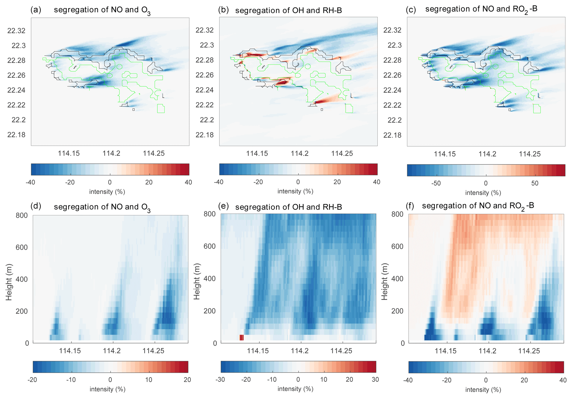
Figure 7Segregation intensities at the first level (a–c) and the vertical cross section along latitude 22.275∘ N (d–f) at hour 4 for the HETF case. The black line shows the urban area, and the green line shows the forest area.
The calculated mean segregation intensities for NO and O3 are −3.21 % and −2.25 % for the low- and high-altitude bands respectively, which is more than 5 times (low band) and 2 times (high band) larger than the HOMF simulation with homogeneous emissions (see details in Table 4). Since the influence of the emissions is stronger in the lowest levels, the segregation intensity is also larger at lower altitudes. In addition to the mean values, the maximum intensity can reach −50 %, implying that the impact of the heterogenous character of the emissions can be very strong at certain locations, specifically in the vicinity of the source regions. For the two other negatively correlated reactions, the mean segregation intensities for RH-A and OH are −3.61 % (low) and −3.20 % (high), and those for NO and RO2-A are −9.79 % and −9.21 %. For the reaction of RH-B with OH, which has both positive and negative intensities as shown in Fig. 7, the mean values are −7.20 % and −10.19 %. Even though the total segregation is characterized by a negative intensity, the maximum positive value of this quantity is higher than 100 %, which occurs near the surface; this may explain why the negative intensity at low altitudes is smaller than the intensity at high altitudes for this reaction. The segregation intensities under the inhomogeneous emission conditions are dependent on the distribution of the emission, so that the numbers cannot be compared directly; however, previous studies also show larger segregation intensities with heterogenous emissions. For instance, Ouwersloot et al. (2011) derive an isoprene segregation intensity of −12.6 % in their heterogeneous case; Kaser et al. (2015) derived intensities as large as −30 % from measurements of isoprene local segregation. Regarding the reaction of NO with RO2-B, the mean segregation intensity at the lower atmospheric levels is negative (−5.15 %) and at higher levels is positive (0.90 %). The small positive value is probably diminished by the negative intensities; therefore, it is smaller when produced in the HOMF simulation with homogeneous surface emissions.
3.3 Influence of the complex terrain
Over the flat terrain, the PBL evolution is mainly controlled by the upward surface heat flux and by the downward heat flux (entrainment) at the top of the PBL. Over the mountains, in addition to the thermally driven forcing, the advection of the flow, the occurrence of mountain waves, and the rotors also play important roles in the turbulence structure (De Wekker and Kossmann, 2015). In order to assess the role of the turbulence generated by the presence of mountains in the segregation between chemical species, we now consider the topography of Hong Kong Island in our model simulations (simulation TERW, TERE, TERS, TERN). The terrain is expected to affect the chemical reactions by changing (1) the turbulent strength and (2) the mean distribution of the chemical species. We first show these two effects by considering the simulation TERW, in which the prevailing mean winds are westerlies. The horizontal wind velocity and the total TKE (the sum of resolved TKE and SGS TKE) with the PBL height along latitude 22.275∘ N are displayed in Fig. 8, which shows how the topography affects the wind field and local turbulence. Compared to the case with flat terrain, the wind speed is smaller at the mountain base and in the valley, while it is significantly larger on the top of the mountains. The derived PBL height mirrors the shape of the terrain (De Wekker and Kossmann, 2015). The PBL height is depressed above the mountain base due to the subsiding circulation associated with the wind system along the slopes; a significant drop in the PBL height is seen over mountain ridges, which is attributed to the Bernoulli effect; and the PBL is elevated over valleys as the mixed layer is lifted by the horizontal advection from the high windward terrain and the local up-valley wind system. The TKE mainly increases behind the steep hills as a result of the flow separation and shear effect produced by the slope (Cao et al., 2012). The TKE associated with the terrain changes the concentration fluctuations of the chemical species.

Figure 8Vertical cross section of the horizontal wind speed (a, b) and total TKE (c, d) along latitude 22.275∘ N at hour 4 for simulations without terrain (left column; HOMF/HETF case) and with terrain (right column; TERW case). The black line indicates the PBL height.
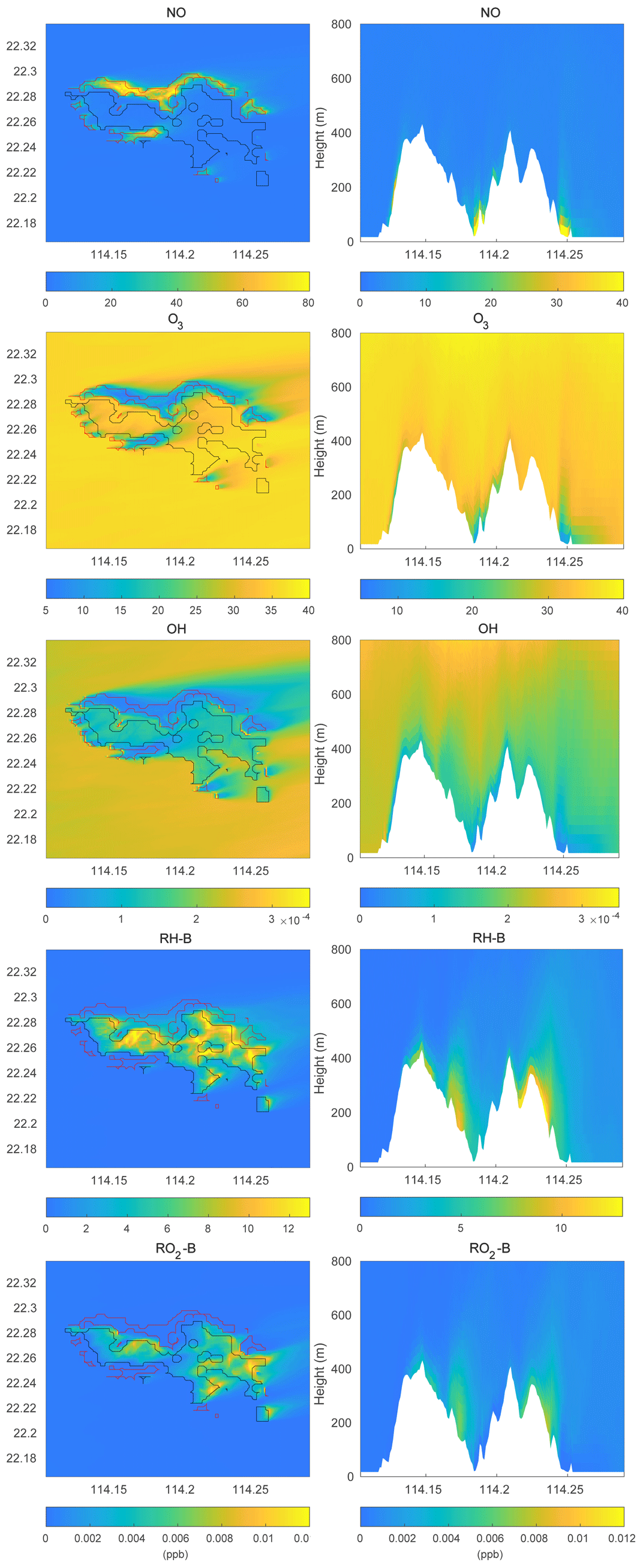
Figure 9Same as Fig. 6 but for the TERW case.
The simulated concentrations of chemical species are shown in Fig. 9. Compared to the concentration distributions from the HETF case without topography (Fig. 6), the overall patterns are similar when represented on quasi-horizontal terrain-following surfaces. There are, however, more defined structures in the concentration fields when taking the influence of the terrain into account. For the vertical cross sections, since the anthropogenic emissions are located in the urbanized areas around the mountains, the concentrations of NO and ozone are high in the valleys and low over the mountains. The concentrations of biogenic RH-B are highest near the surface of the mountains since this organic species is emitted by the trees located on the slopes of the mountains. The vertical distribution of OH is low near the surface everywhere above Hong Kong Island because it is depleted by both anthropogenic and biogenic species; however, the OH concentration is particularly low in the valleys because the anthropogenic species (CO and RH-A) consume large quantities of OH.
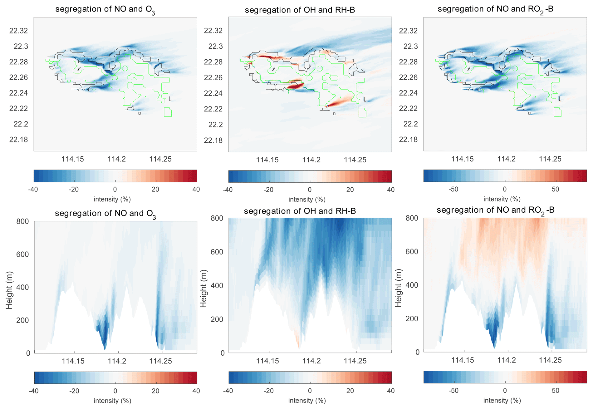
Figure 10Same as Fig. 7 but for the TERW case.
Figure 10 shows the calculated segregation intensities for three different reactions under consideration in this study. As for the mean concentration and the TKE distributions, the structure of the segregation intensities changes with the topography. For the distributions near the ground, it shares patterns similar to those found in the HETF case, since the near-surface chemical concentrations are similar in the two model experiments. For the vertical structures, the topography not only lifts the patterns by the height of the terrain, but it also changes the strength of the segregation intensities. For the reaction between NO and O3, the calculated mean segregation intensity is −3.14 % in the 0–500 m layer and −2.40 % in the 500–800 m layer. These values are similar to those derived in the HETF simulation, implying that the terrain does not substantially change the mean segregation. Because of the complexity of the topography with a large number of mountain ridges and valleys (and hence some possible compensating effects), the resulting influence of the topography appears on average to be relatively small. However, the local maximum intensity is −59.18 %, which is larger than the −50.44 % obtained in the HETF case. The terrain impact on the reaction of RH-A and OH and NO and RO2-A is the same as the reaction of NO with O3. For the reaction of OH and RH-B, the averaged intensity for the low-altitude band is −5.86 % and is therefore smaller than the −7.20 % obtained in the HETF case; however, the mean segregation intensity is −11.16 % for the higher altitude band, which is larger than in the HETF calculation. For the reaction between NO with RO2-B, negative segregation intensities are found mainly below 500 m, and positive intensities are derived above 500 m. The separation height is raised by about 300 m compared to the HETF case (no topography). The mean intensity below and above 500 m is −5.60 % and 1.65 % respectively.
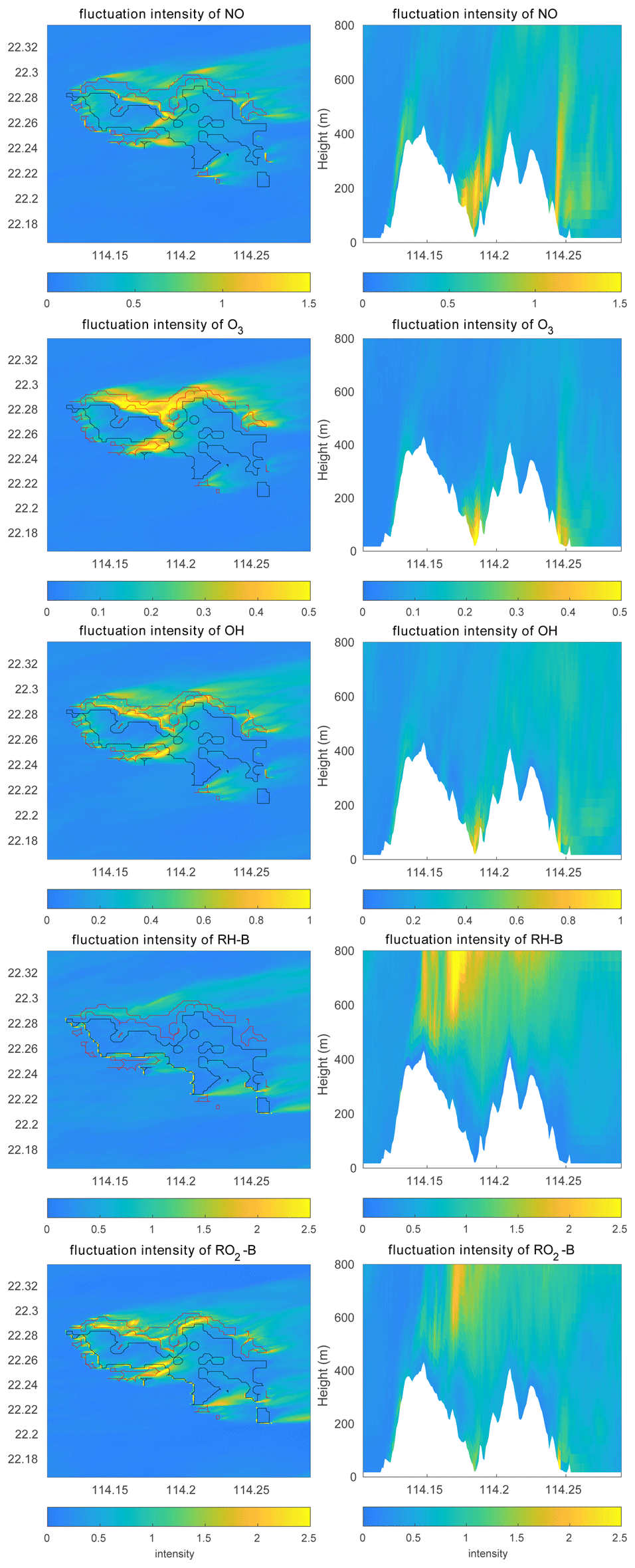
Figure 11Concentration fluctuation intensities (variance divided by the mean concentration) at the first level (left panels) and the vertical cross section along latitude 22.275∘ N (right panels) at hour 4 for TERW case. The red line shows the urban area, and the black line shows the forest area.
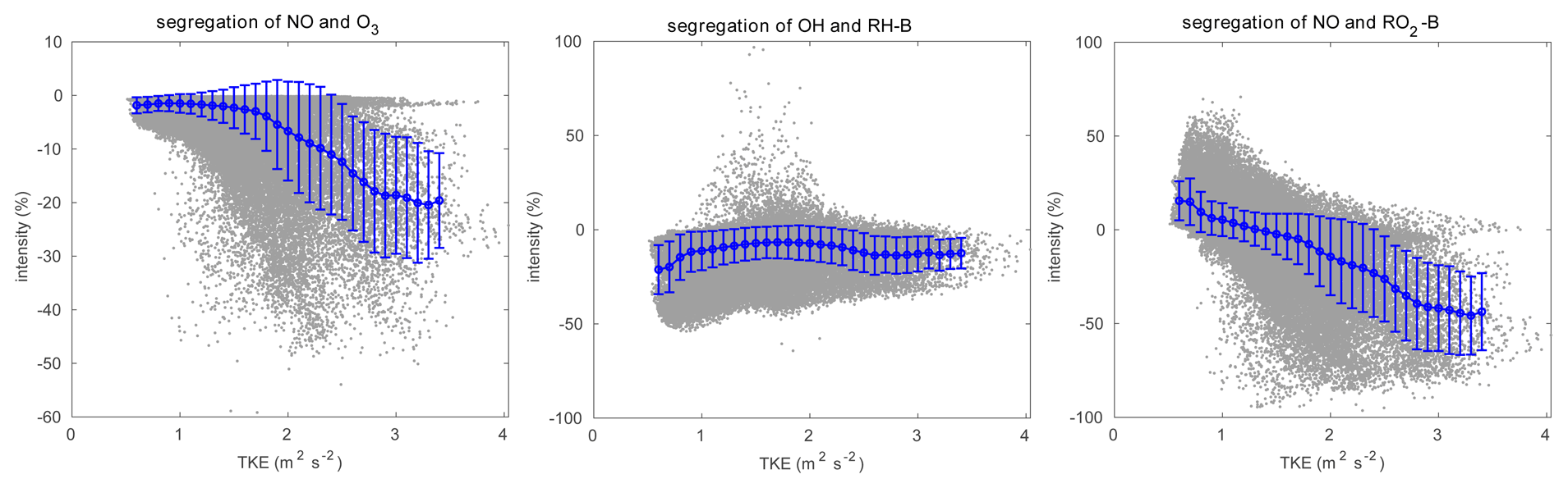
Figure 12Relationship between segregation intensity and TKE. The grey dots represent the raw data, and the blue dots are the mean value in every TKE bin with a width of 0.1 m2 s−2. The error bars show the standard deviations.
The concentration fluctuation intensities for the selected species are represented in Fig. 11. As defined in Sect. 2.4, the concentration fluctuation intensity depends on both the mean concentration and the intensity of the turbulence. For the anthropogenic emitted species such as NO, with high concentrations in the urban area, the fluctuation generated by the turbulence is relatively large because of the large concentration gradients in this region. The NO concentration fluctuation intensity is highest in the urban regions where fluctuations dominate, for instance, in the valley between the two mountain peaks and at the eastern side of the hills (the leeward slopes). This is consistent with the TKE distribution. In the case of O3, which is consumed by NO, the concentration is low in the urban area; however, the gradient in the concentration is large, and therefore the fluctuation intensity is strong. The situation is similar for OH. For the biogenic species RH-B and its secondary product RO2-B, the calculated concentration fluctuation intensity is low in their source region, implying that the TKE above the mountain is relatively small, and thus the concentration fluctuation intensity is inversely related to the concentration of the two species. As shown in Eq. (9), the sign of the segregation is controlled by the correlation factor r, and the segregation intensity depends on the concentration fluctuation intensity of both reactants. For the reaction of NO and O3, because the concentration fluctuation intensity for both species is strong in the urban region, the segregation is strong in this area, especially in areas where TKE is large. For the reaction of RH-B and OH, the segregation intensity is more dependent on the concentration fluctuation intensity of RH-B, which has larger values. The segregation intensity for the reaction of NO and RO2-B is controlled by NO at low altitudes, but it is dominated by RO2-B above 500 m. The relationship between the segregation intensity and TKE is shown in Fig. 12. For the reaction between NO and O3 and the reaction between NO and RO2-B, the segregation intensities generally increase with TKE, which is similar to the findings of Dlugi et al. (2014). This supports our hypothesis that terrain affects the segregation through the turbulent strength. However, there is no clear relationship between segregation intensity and TKE for the reaction between RH-B and OH. As discussed above, the source of RH-B is located on the top of the mountains where the TKE is relatively small, so the influence of TKE is overwhelmed by the emission distribution.
Table 5List of the calculated segregation differences between the experiments TERW and the HETF run for the center region (14 × 14 km2) of the domain.

To better analyze the impact of the topography, the differences of the segregation between the experiment TERW and HETF are shown in Fig. 13. The statistics of the differences are listed in Table 5. It shows that, even though the averaged intensities do not change substantially, the local influence of the terrain is important. The maximum differences are 57.95 %, 49.79 %, 154.03 %, 85.73 %, and 186.42 % for the five reactions under consideration. For the reaction between NO and O3, the negative intensity increases mainly in the valley near the center and on the east edge of the island and decreases in the north of the island and on the top of the mountains. The terrain impact on the reaction of NO with RO2-B is similar to what is found for the NO–O3 reaction near the surface, but it is different in the upper layers, where the positive segregation becomes stronger. The situation is more complicated for the reaction between OH and RH-B in the surface layer: the strongest influence of the terrain appears at the boundary between the urban and forest emissions, where the segregation intensity is largest. For the vertical distribution, the negative segregation decreases at most places in the lower levels, except to the west of the mountains and on the windward side of the slope. At higher altitudes, the negative segregation intensity increases.
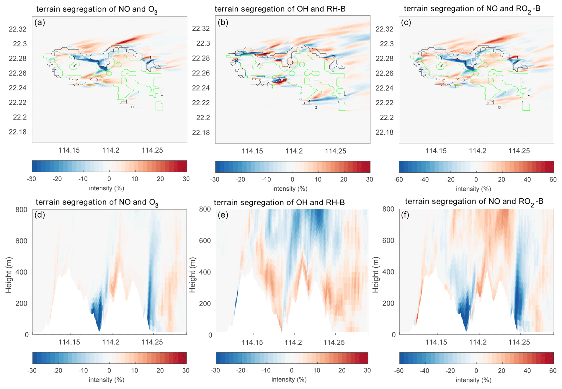
Figure 13Differences of the segregation intensity between TERW and HETF (TERW − HETF) at the first level (a–c) and the vertical cross section along latitude 22.275∘ N (d–f). The black line shows the urban area, and the green line shows the forest area.
The differences in the intensities of the concentration fluctuations between the simulations with and without topography are shown in Fig. 14. The concentration fluctuation intensities for NO, O3, and OH are all increased in the valleys and on the leeward side of the mountains at the east of the island. This results from the increase in the concentration gradient of these species and from the strong TKE created by the terrain. In contrast, the concentration fluctuation intensity of RH-B decreases in the region where TKE is large because the source of the RH-B is not located in an area where turbulence is strong. Thus, the model shows that the concentration fluctuation intensity of a chemical species is dependent on the emissions, the turbulent kinetic energy, and the relative location of the two terms. When we connect the segregation induced by topography with the differences of the concentration fluctuation intensities, we find that the segregation becomes stronger in areas where the concentration fluctuation intensities of both reactants increase, while it is weaker where their concentration fluctuation intensities decrease. The segregation intensity is dominated by the chemical species that has the largest concentration fluctuation intensity if the changes by the terrain of this latter quantity are opposite for the two reactants.
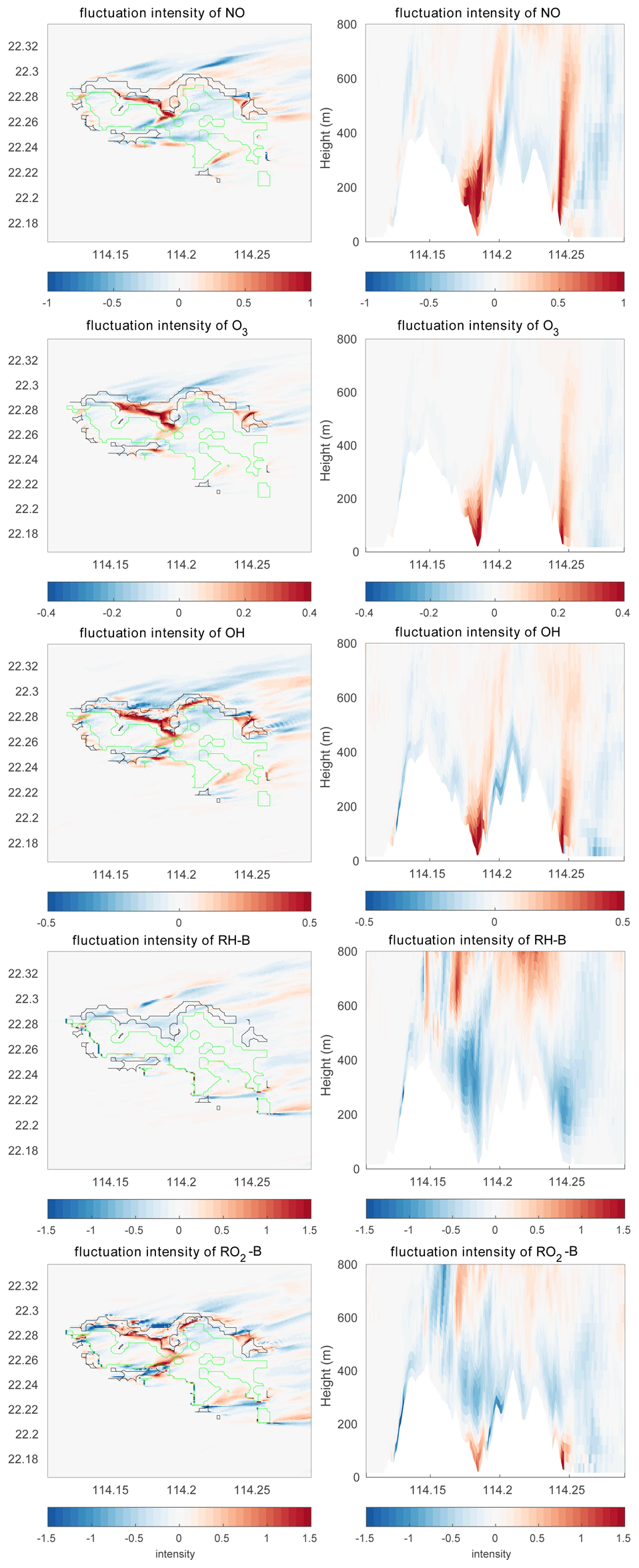
Figure 14Differences of the concentration fluctuation intensity (variance divided by the mean concentration) between TERW and HETF (TERW – HETF) at the first level (left panels) and the vertical cross section along latitude 22.275 °N (right panels). The black line shows the urban area, and the green line shows the forest area.
3.4 Impact on the ozone production and destruction
Finally, we estimate the impact of the segregation mechanisms on the formation of a key secondary species: ozone. In our chemical scheme, the limiting chemical processes in the photochemical production of this molecule are provided by the three reactions by which peroxy radicals convert NO into NO2 (see Table 1).
Here REST-A and REST-B represent possible secondary products that are not further considered in our simplified analysis. The photolysis of NO2 produced by the three reactions leads directly to the formation of ozone, and the production rate of odd oxygen (Ox= O3 + NO2), P(Ox), is expressed in a turbulent medium by
Here the brackets 〈〉 refer to the time-averaged concentration at each model grid point. Reaction rates k7, k17, and k20 and segregation intensities I7, I17, and I20 correspond to Reactions (R7), (R17), and (R20), respectively. Thus, the production rate of odd oxygen is not only determined by the product of the mean concentration of nitric oxide and peroxy radicals, but also by the chemical covariance between the fluctuations of these species.
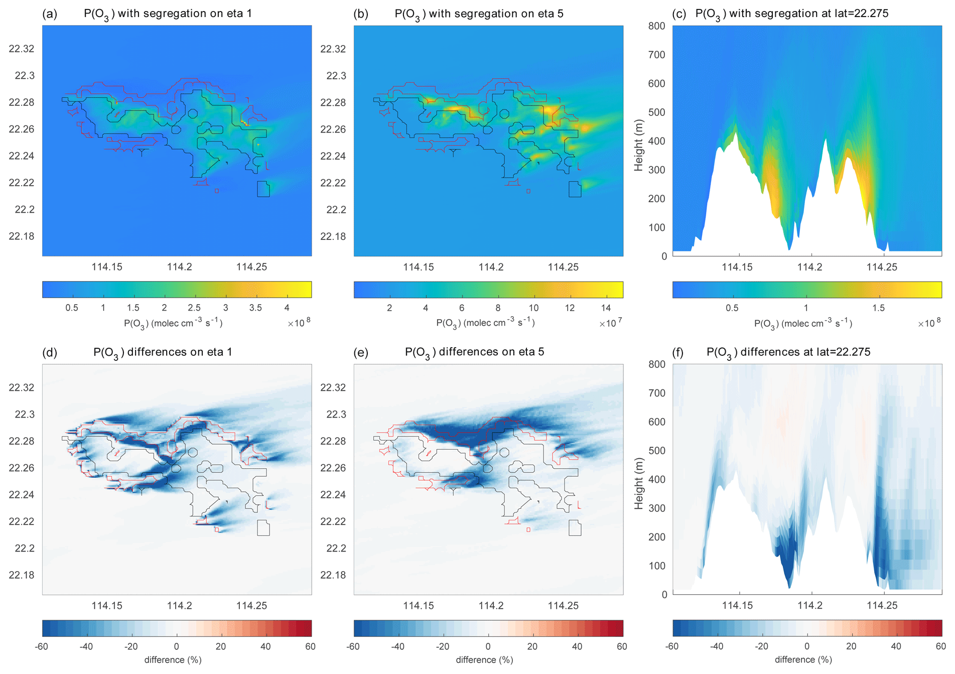
Figure 15(a–c) Production rate of ozone (molec. cm−3 s−1) in and around Hong Kong Island. (a) Values at the lowest model level, (b) values at model level 5, and (c) values as a function of height along the constant latitude of 22.275∘ N. (d–f) Same but for the percentage difference between ozone production rates with and without segregation effects taken into account.
The photochemical loss rate of Ox is due primarily to the following reactions:
with a loss rate in the turbulent medium expressed as
Figure 15a–b show the mean ozone production rate on model level 1 (at the surface following the terrain topography) and at model level 5 (about 200 m above the surface), with the effect of segregation included. A cross section of the same quantity is shown across Hong Kong Island along latitude 22.275∘ N in Fig. 15c. The figure highlights the complexity of the spatial patterns characterizing the formation of odd oxygen with the existence of values generally peaking at the northern and northeastern coasts of the island. A peak in the production is also found in the central valley and on the leeward slopes of the hills. Figure 15d–f show that the odd oxygen production rate resulting from the segregation effect is reduced by values that can reach more than 60 % locally, specifically along the coasts or in the valleys where the anthropogenic emissions (e.g., traffic) are highest. On average, the production rate of Ox over the central area (14 × 14 km2) of the inner domain is reduced by 8 % to 12 % in the first 1000 m of the boundary layer (Fig. 16). The change in the Ox loss rate is small and positive due to the positive correlation between ozone and OH and between ozone and HO2 but the negative correlation between O(1D) and water vapor.
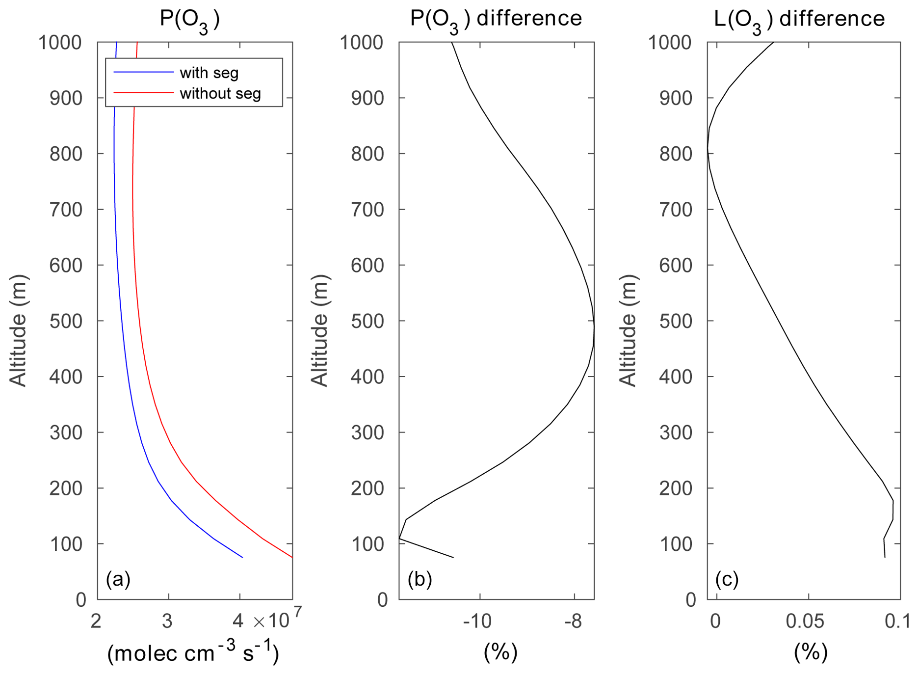
Figure 16(a) Vertical distribution of the ozone production rate (molec. cm−3 s−1) averaged over the central 14×14 km2 of the inner domain, with the effect of segregation taken into account (blue curve) or ignored (red curve). (b, c) Percentage difference between the two cases for the photochemical production and destruction rates.
3.5 Difference with the wind directions
Additional simulations were performed to assess if the prevailing wind direction affects the segregation intensity since different wind directions are expected to produce different spatial distributions of the turbulence generated by the topography. The calculated statistics are shown in Table 4. For the reaction between NO and O3, the mean segregation intensity in the lower layer is −3.14 %, −3.04 %, −2.78 %, and −2.83 %, respectively, for mean winds blowing from the west, east, south, and north directions; the corresponding intensities for the higher altitudes are −2.40 %, −2.45 %, −1.59 %, and −2.84 %, respectively. The largest segregation intensity for the lower level is from the west wind, while that for the higher level is from the north wind. The smallest segregation intensity is from the south wind for both altitude bands. For the reaction of RH-A with OH, the calculated mean intensities for the west, east, south, and north winds are −3.54 %, −3.39 %, −3.15 %, and −3.76 % for the lower altitudes and −3.47 %, −3.41 %, −2.17 %, and −4.39 % for the higher altitudes. The strongest segregation is generated by the north wind and the weakest by the south wind. The same qualitative result is found for the reaction between NO and RO2-A. In this case, the mean intensities are −9.56 %, −9.07 %, −8.63 %, and −10.08 % for the low level and −9.79 %, −9.51 %, −6.86 %, and −12.32 % for the high level in the four wind directions. For the reaction of RH-B with OH, the mean intensities are −5.86 %, −5.01 %, −6.62 %, and −8.50 % for the four wind directions at the low bands and −11.16 %, −10.58 %, −10.08 %, and −15.8 % for the high-altitude band. The east wind produces the strongest segregation, and the north wind has the lowest intensity at the low level; the south and the north winds give the highest and the lowest segregation intensity at the high level, respectively. For the reaction between NO and RO2-B, the averaged intensities are −5.60 %, −6.03 %, −4.15 %, and −2.91 % at low altitudes and 1.65 %, 1.04 %, 3.93 %, and 5.03 % at high altitudes. The negative intensity at the low level is largest when the wind is from the east and smallest when the wind is from the north. The positive segregation is strongest for the north wind and weakest for the east wind.
As discussed in the previous section, the large TKE appears at the leeward side of the hills, resulting from the flow recirculation and wind shear effect. However, TKE is high only at certain specific locations, while its magnitude is similar for the four experiments in the whole domain. On the other hand, the large TKE is expected to have a strong impact on the chemical reactions at the locations where the two reactants are characterized by large concentration gradients. This means that the influence of the TKE is dependent on the distribution of the chemical species too. The different wind directions seem to have a small impact on the mean segregation in our simulations, and this is probably because the topography is too complex, with a large number of mountain ridges and valleys, and therefore the influences are canceled out when considering the domain as a whole.
The large-eddy simulations presented here were performed to study how urban air pollution behaves at the turbulent scale, a scale that cannot be resolved by global or regional models. The segregation effect on the chemical reactions resulting from inefficient turbulent mixing was analyzed. The region of Hong Kong Island offers an interesting situation to conduct such a study because of the highly inhomogeneous surface emissions of reactive species and the complex topography.
The inhomogeneity in the emissions tends to increase the segregation intensities by a factor of 2–5 compared to the simulations performed with homogeneous emissions. In some cases, the heterogeneity in the emissions can even generate a change in the sign of the segregation, resulted from the separated sources of the two reactants. In our chemical mechanism, the reaction between NO and RO2-B is not affected by segregation if NO and RH-B emissions are co-located as in the HOMF case, but a separation between the location of the anthropogenic and biogenic emissions produces a segregation between NO and RH-B at low altitudes and thus a reduction in the effective rate at which the reaction between NO and RO2-B proceeds.
The topography plays a substantial role in the chemical reactions by influencing the turbulence distribution and intensity and hence impacting the concentration distributions. Near the mountains, the TKE increases on the leeward side of the slope, leading to more intense concentration fluctuations for the species with large concentration gradients. For the species with large spatial concentration gradients in areas where turbulence is weak (e.g., RH-B on the top of the mountain), the intensity of the concentration fluctuation is not enhanced.
The topography has important impact on the segregation intensity locally, especially if the terrain induces strong TKE values in areas where emissions are intense. The differences in the segregation intensities caused by the terrain can be larger than 50 % at certain locations; however, the mean influence of the topography over the whole domain remains relatively small.
Simulations performed for varied wind directions show few differences in the mean segregation intensities because the values of the TKE generated by the topography are high only at a limited number of locations (generally the leeward side of the mountains), with little impact on the spatially averaged intensity of the segregation.
In the particular setting of our model for Hong Kong Island, with heterogeneous emissions and mountainous topography, the averaged segregation intensities from the surface to 500 m are of the order of −3 %, −3.5 %, −6 %, −9.5 %, and −5.5 % for the NO + O3, OH + RH-A, OH + RH-B, NO + RO2-A, and NO + RO2-B reactions, respectively. At 500 m above the surface, segregation reduces the ozone formation by 8 % compared to a case with complete mixing. At 100 m above the surface, this reduction is close to 12 %.
The conceptual model presented here and applied to a region with very inhomogeneous conditions highlights the importance of segregation between reactive species, in particular in the convective planetary boundary layer. Segregation, whose intensity is a function of the chemical and turbulent time constants, occurs at spatial and temporal scales that are not resolved by usual global and regional chemical transport models. The study suggests that, when used in coarse-resolution models, the chemical rate constants measured in the laboratory should be adjusted in the boundary layer to correct for the subgrid segregation effect (see Eq. 8). This effect is ignored by these models because they assume complete mixing of reactive species within each grid cell.
The code or data used in this study are available upon request from the corresponding author.
YW designed and performed the experiments. YW and YFM analyzed the simulations. YW, YFM, and GPB wrote the article. GPB initiated the idea of the work. GPB and TW provided guidance to YW. DME and MB provided advice and support on the setup of the LES. In addition, DME, CWYL, and MB contributed to the editing of the article.
The authors declare that they have no conflict of interest.
Yong-Feng Ma's contribution to this work was supported by the Shenzhen Science & Technology Program (grant no. KQTD20180411143441009). The National Center for Atmospheric Research is sponsored by the US National Science Foundation. We would like to acknowledge high-performance computing support from NCAR Cheyenne.
This research has been supported by the Hong Kong Research Grants Council (grant no. T24-504/17-N). The article processing charges for this open-access publication were covered by the Hong Kong Research Grants Council (grant no. T24-504/17-N).
This paper was edited by Jason West and reviewed by two anonymous referees.
Anfossi, D., Rizza, U., Mangia, C., Degrazia, G. A., and Pereira Marques Filho, E.: Estimation of the ratio between the Lagrangian and Eulerian time scales in an atmospheric boundary layer generated by large eddy simulation, Atmos. Environ., 40, 326–337, https://doi.org/10.1016/j.atmosenv.2005.09.041, 2006.
Auger, L. and Legras, B.: Chemical segregation by heterogeneous emissions, Atmos. Environ., 41, 2303–2318, https://doi.org/10.1016/j.atmosenv.2006.11.032, 2007.
Barth, M. C., Kim, S.-W., Wang, C., Pickering, K. E., Ott, L. E., Stenchikov, G., Leriche, M., Cautenet, S., Pinty, J.-P., Barthe, Ch., Mari, C., Helsdon, J. H., Farley, R. D., Fridlind, A. M., Ackerman, A. S., Spiridonov, V., and Telenta, B.: Cloud-scale model intercomparison of chemical constituent transport in deep convection, Atmos. Chem. Phys., 7, 4709–4731, https://doi.org/10.5194/acp-7-4709-2007, 2007.
Brasseur, G. P. and Jacob, D. J.: Modeling of Atmospheric Chemistry, Cambridge University Press, Cambridge, 2017.
Cao, S., Wang, T., Ge, Y., and Tamura, Y.: Numerical study on turbulent boundary layers over two-dimensional hills–Effects of surface roughness and slope, J. Wind Eng. Ind. Aerodyn., 104, 342–349, https://doi.org/10.1016/j.jweia.2012.02.022, 2012.
Damköhler G.: Influence of turbulence on the velocity of flames in gas mixtures, Z. Elektrochem., 46, 601–626, 1940.
Danckwerts, P. V.: The definition and measurement of some characteristics of mixtures, Appl. Sci. Res., 3, 279–296, https://doi.org/10.1007/BF03184936, 1952.
Deardorff, J. W.: A numerical study of three-dimensional turbulent channel flow at large Reynolds numbers, J. Fluid Mech., 41, 453–480, https://doi.org/10.1017/S0022112070000691, 1970.
De Wekker, S. F. and Kossmann, M.: Convective boundary layer heights over mountainous terrain – A review of concepts, Front. Earth Sci., 3, 77, https://doi.org/10.3389/feart.2015.00077, 2015.
Dlugi, R., Berger, M., Zelger, M., Hofzumahaus, A., Rohrer, F., Holland, F., Lu, K., and Kramm, G.: The balances of mixing ratios and segregation intensity: a case study from the field (ECHO 2003), Atmos. Chem. Phys., 14, 10333–10362, https://doi.org/10.5194/acp-14-10333-2014, 2014.
Dlugi, R., Berger, M., Mallik, C., Tsokankunku, A., Zelger, M., Acevedo, O. C., Bourtsoukidis, E., Hofzumahaus, A., Kesselmeier, J., Kramm, G., Marno, D., Martinez, M., Nölscher, A. C., Ouwersloot, H., Pfannerstill, E. Y., Rohrer, F., Tauer, S., Williams, J., Yáñez-Serrano, A.-M., Andreae, M. O., Harder, H., and Sörgel, M.: Segregation in the Atmospheric Boundary Layer: The Case of OH – Isoprene, Atmos. Chem. Phys. Discuss. [preprint], https://doi.org/10.5194/acp-2018-1325, 2019.
ESA: Land Cover CCI Product User Guide Version 2, Tech. Rep., available at: http://maps.elie.ucl.ac.be/CCI/viewer/download/ESACCI-LC-Ph2-PUGv2_2.0.pdf (last access: 1 June 2020), 2017.
Ganzeveld, L. and Lelieveld, J.: Dry deposition parameterization in a chemistry general circulation model and its influence on the distribution of reactive trace gases, J. Geophys. Res., 100, 20999–21012, https://doi.org/10.1029/95JD02266, 1995.
Kaser, L., Karl, T., Yuan, B., Mauldin, R. L., Cantrell, C. A., Guenther, A. B., Patton, E. G., Weinheimer, A. J., Knote, C., Orlando, J., Emmons, L., Apel, E., Hornbrook, R., Shertz, S., Ullmann, K., Hall, S., Graus, M., de Gouw, J., Zhou, X., and Ye, C.: Chemistry-turbulence interactions and mesoscale variability influence the cleansing efficiency of the atmosphere, Geophys. Res. Lett., 42, 10894–10903, https://doi.org/10.1002/2015GL066641, 2015.
Kessler, E.: On the distribution and continuity of water substance in atmospheric circulations, Am. Meteorol. Soc., Boston, MA, https://doi.org/10.1007/978-1-935704-36-2_1, 1969.
Kim, S. W., Barth, M. C., and Trainer, M.: Impact of turbulent mixing on isoprene chemistry, Geophys. Res. Lett., 43, 7701–7708, https://doi.org/10.1002/2016GL069752, 2016.
Kirkil, G., Mirocha, J., Bou-Zeid, E., Chow, F., K., and Kosovi'c, B.: Implementation and evaluation of dynamic subfilter-scale stress models for large-eddy simulation using WRF, Mon. Weather Rev., 140, 266–284, https://doi.org/10.1175/MWR-D-11-00037.1, 2012.
Komori, S., Hunt, J. C. R., Kanzaki, T., and Murakami, Y.: The effects of turbulent mixing on the correlation between two species and on concentration fluctuations in non-premixed reacting flows, J. Fluid Mech. Digit. Arch., 228, 629–659, https://doi.org/10.1017/S0022112091002847, 1991.
Kosović, B., Mirocha, J. D., and Lundquist, K. A.: Validation of large-eddy simulation of flows over complex terrain with the weather research and forecasting model, 21st Symposium on Boundary Layers and Turbulence, 8–13 June 2014, Leeds, UK, 3A.3, 2014.
Kramm, G. and Meixner, F. X.: On the dispersion of trace species in the atmospheric boundary layer: a re-formulation of the governing equations for the turbulent flow of the compressible atmosphere, Tellus A, 52, 500–522, https://doi.org/10.3402/tellusa.v52i5.12279, 2000.
Krol, M. C., Molemaker, M. J., and Vilà-Guerau De Arellano, J.: Effects of turbulence and heterogeneous emission on photochemically active species in the convective boundary layer, J. Geophys. Res., 105, 6871–6884, https://doi.org/10.1029/1999JD900958, 2000.
Li, C. W. Y., Brasseur, G. P., Schmidt, H., and Mellado, J. P.: Error induced by neglecting subgrid chemical segregation due to inefficient turbulent mixing in regional chemical-transport models in urban environments, Atmos. Chem. Phys., 21, 483–503, https://doi.org/10.5194/acp-21-483-2021, 2021.
Li, Y., Barth, M. C., Chen, G., Patton, E. G., Kim, S. W., Wisthaler, A., Mikoviny, T., Fried, A., Clark, R., and Steiner, A. L.: Large-eddy simulation of biogenic VOC chemistry during the DISCOVER-AQ 2011 campaign, J. Geophys. Res., 121, 8083–8105, https://doi.org/10.1002/2016JD024942, 2016.
Li, Y., Barth, M. C., Patton, E. G., and Steiner, A. L.: Impact of in-cloud aqueous processes on the chemistry and transport of biogenic volatile organic compounds, J. Geophys. Res., 122, 11131–11153, https://doi.org/10.1002/2017JD026688, 2017.
Li, Y., Barth, M. C., and Steiner, A. L.: Comparing turbulent mixing of atmospheric oxidants across model scales, Atmos. Environ., 199, 88–101, https://doi.org/10.1016/j.atmosenv.2018.11.004, 2019.
Liang, J., Guo, Q., Zhang, Z., Zhang, M., Tian, P., and Zhang, L.: Influence of complex terrain on near-surface turbulence structures over Loess Plateau, Atmosphere-Basel, 11, 930, https://doi.org/10.3390/atmos11090930, 2020.
Liu, S. and Liang, X. Z.: Observed diurnal cycle climatology of planetary boundary layer height, J. Climate, 23, 5790–5809, https://doi.org/10.1175/2010JCLI3552.1, 2010.
Mapes, B. E., Warner, T. T., Xu, M., and Gochis, D. J.: Comparison of cumulus parameterizations and entrainment using domain-mean wind divergence in a regional model, J. Atmos. Sci., 61, 1284–1295, https://doi.org/10.1175/1520-0469(2004)061<1284:COCPAE>2.0.CO;2, 2004.
Moeng, C.-H., Dudhia, J., Klemp, J., and Sullivan, P.: Examining two-way grid nesting for large eddy simulation of the PBL using the WRF model, Mon. Weather Rev., 135, 2295–2311, https://doi.org/10.1175/mwr3406.1, 2007.
Molemaker, M. J. and Vilà-Guerau de Arellano, J.: Control of chemical reactions by convective turbulence in the boundary layer, J. Atmos. Sci., 55, 568–579, https://doi.org/10.1175/1520-0469(1998)055<0568:COCRBC>2.0.CO;2, 1998.
Muñoz-Esparza, D., Kosović, B., García-Sánchez, C., and van Beeck, J.: Nesting turbulence in an offshore convective boundary layer using large-eddy simulations, Bound.-Lay. Meteorol., 151, 453–478, https://doi.org/10.1007/s10546-014-9911-9, 2014.
Ouwersloot, H. G., Vilà-Guerau de Arellano, J., van Heerwaarden, C. C., Ganzeveld, L. N., Krol, M. C., and Lelieveld, J.: On the segregation of chemical species in a clear boundary layer over heterogeneous land surfaces, Atmos. Chem. Phys., 11, 10681–10704, https://doi.org/10.5194/acp-11-10681-2011, 2011.
Patton, E. G., Davis, K. J., Barth, M. C., and Sullivan, P. P.: Decaying scalars emitted by a forest canopy: a numerical study, Bound.-Lay. Meteorol., 100, 91–129, https://doi.org/10.1023/A:1019223515444, 2001.
Rotach, M. W., Gohm, A., Lang, M. N., Leukauf, D., Stiperski, I., and Wagner, J. S.: On the vertical exchange of heat, mass, and momentum over complex, mountainous terrain, Front. Earth Sci., 3, 76, https://doi.org/10.3389/feart.2015.00076, 2015.
Schumann, U.: Large-eddy simulation of turbulent diffusion with chemical reactions in the convective boundary layer, Atmos. Environ., 23, 1713–1727, https://doi.org/10.1016/0004-6981(89)90056-5, 1989.
Seidel, D. J., Ao, C. O., and Li, K.: Estimating climatological planetary boundary layer heights from radiosonde observations: Comparison of methods and uncertainty analysis, J. Geophys. Res., 115, D16113, https://doi.org/10.1029/2009JD013680, 2010.
Shu, Z. R., Li, Q. S., and Chan, P. W.: Statistical analysis of wind characteristics and wind energy potential in Hong Kong, Energy Convers. Manag., 101, 644–657, https://doi.org/10.1016/j.enconman.2015.05.070, 2015.
Skamarock, W. C. and Klemp, J. B.: A time-split nonhydrostatic atmospheric model for weather research and forecasting applications, J. Comput. Phys., 227, 3465–3485, https://doi.org/10.1016/j.jcp.2007.01.037, 2008.
Skamarock, W. C., Klemp, J. B., Dudhia, J., Gill, D. O., Liu, Z., Berner, J., Wang, W., Powers, J. G., Duda, M. G., Barker, D. M., and Huang, X.-Y.: A Description of the Advanced Research WRF Version 4, NCAR Tech. Note NCAR/TN-556+STR, 145 pp., https://doi.org/10.5065/1dfh-6p97, 2019.
Smagorinsky, J.: General circulation experiments with the primitive equations: I. the basic experiment, Mon. Weather Rev., 91, 99–164, https://doi.org/10.1175/1520-0493(1963)091<0099:GCEWTP>2.3.CO;2, 1963.
Takaku, J., Tadono, T., and Tsutsui, K.: Generation of High Resolution Global DSM from ALOS PRISM, Int. Arch. Photogramm. Remote Sens. Spatial Inf. Sci., XL-4, 243–248, https://doi.org/10.5194/isprsarchives-XL-4-243-2014, 2014.
Verver, G. H. L., van Dop, H., and Holtslag, A. A. M.: Turbulent mixing and the chemical breakdown of isoprene in the atmospheric boundary layer, J. Geophys. Res., 105, 3983–4002, https://doi.org/10.1029/1999JD900956, 2000.
Vilà-Guerau de Arellano, J. and Duynkerke, P. G.: Second-order closure study of the covariance between chemically reactive species in the surface layer, J. Atmos. Chem., 16, 145–155, https://doi.org/10.1007/BF00702784, 1993.
Vinuesa, J. F. and Vilà-Guerau de Arellano, J.: Introducing effective reaction rates to account for the inefficient mixing of the convective boundary layer, Atmos. Environ., 39, 445–461, https://doi.org/10.1016/j.atmosenv.2004.10.003, 2005.
Vinuesa, J. F. and Vilà-Guerau de Arellano, J.: Fluxes and (co-)variances of reacting scalars in the convective boundary layer, Tellus B, 55, 935–949, https://doi.org/10.3402/tellusb.v55i4.16382, 2011.
Wu, Z., Wang, X., Chen, F., Turnipseed, A. A., Guenther, A. B., Niyogi, D., Charusombat, U., Xia, B., Munger, J. W., and Alapaty, K.: Evaluating the calculated dry deposition velocities of reactive nitrogen oxides and ozone from two community models over a temperate deciduous forest, Atmos. Environ., 45, 2663–2674, https://doi.org/10.1016/j.atmosenv.2011.02.063, 2011.
Yamaguchi, T. and Feingold, G.: Technical note: Large-eddy simulation of cloudy boundary layer with the Advanced Research WRF model, J. Adv. Model. Earth Syst., 4, M09003, https://doi.org/10.1029/2012MS000164, 2012.