Comparative study on immersion freezing utilizing single-droplet levitation methods

Immersion freezing experiments were performed utilizing two distinct single-droplet levitation methods. In the Mainz vertical wind tunnel, supercooled droplets of 700 µm diameter were freely floated in a vertical airstream at constant temperatures ranging from −5 to −30 ^∘C, where heterogeneous freezing takes place. These investigations under isothermal conditions allow the application of the stochastic approach to analyze and interpret the results in terms of the freezing or nucleation rate. In the Mainz acoustic levitator, 2 mm diameter drops were levitated while their temperature was continuously cooling from +20 to −28 ^∘C by adapting to the ambient temperature. Therefore, in this case the singular approach was used for analysis. From the experiments, the densities of ice nucleation active sites were obtained as a function of temperature. The direct comparison of the results from two different instruments indicates a shift in the mean freezing temperatures of the investigated drops towards lower values that was material-dependent. As ice-nucleating particles, seven materials were investigated; two representatives of biological species (fibrous and microcrystalline cellulose), four mineral dusts (feldspar, illite NX, montmorillonite, and kaolinite), and natural Sahara dust. Based on detailed analysis of our results we determined a material-dependent parameter for calculating the freezing-temperature shift due to a change in cooling rate for each investigated particle type. The analysis allowed further classification of the investigated materials to be described by a single- or a multiple-component approach. From our experiences during the present synergetic studies, we listed a number of suggestions for future experiments regarding cooling rates, determination of the drop temperature, purity of the water used to produce the drops, and characterization of the ice-nucleating material. The observed freezing-temperature shift is significantly important for the intercomparison of ice nucleation instruments with different cooling rates.

1 Introduction

Immersion freezing is considered to be the most effective nucleation process for ice particle production in mixed-phase clouds (Diehl and Grützun, 2018). The ice nucleation abilities of atmospheric particles have been investigated very intensively in the last decades (Hoose and Möhler, 2012). Besides in situ measurements, laboratory-based investigation techniques are widely used to discover the basic physical and chemical processes and properties of ice-nucleating particles (INPs). Laboratory immersion freezing experiments aim to characterize of the temperature-dependent ice nucleation ability of different types of INPs under controlled conditions. The ice nucleation efficiency of INPs is commonly expressed in terms of ice-nucleation-active-site (INAS) density n_s(T). This is calculated from the experimentally determined total number of nucleation events per unit surface area of the particles. INAS density is used to represent the number of ice-active sites on the particles that are active between 0 ^∘C and the subzero temperature T (DeMott, 1995; Connolly et al., 2009; Murray et al., 2012; Hoose and Möhler, 2012). Another important parameter employed for describing the INP nucleation ability is the nucleation rate coefficient, i.e., the probability of nucleation at a certain temperature per unit time per unit surface area of the particle (Vali, 2014). The nucleation rate coefficient is determined using the classical nucleation theory on experiments under isothermal conditions (e.g., Rigg et al., 2013; Murray et al., 2011; Niedermeier et al., 2010).

Intercomparisons of measurement techniques revealed a wide scatter of measured ice nucleation activities of particles. This is due to differences in the measuring methods employed by the different instruments and the diversity in the sample preparation at different research sites. One essential and still-not-understood discrepancy arises between dry-dispersion and aqueous-suspension measurement techniques (Hiranuma et al., 2019). In the former, experiments employ water vapor condensation onto dry-dispersed particles followed by droplet freezing (e.g., cloud chambers, continuous-flow diffusion chambers), while the latter denotes experiments starting with test samples pre-suspended in water before cooling (e.g., freezing arrays, drop levitators). Several studies have focused on identifying potential reasons of this data diversity. Recently, two major international research activities were conducted and produced a large number of new data and results: one organized around the German INUIT (Ice Nucleation Research Unit) research community and the FIN (Fifth International Ice Nucleation Workshop). These intercomparison campaigns revealed data diversity over several orders of magnitude in n_s already among aqueous-suspension techniques also in case of a recommended protocol for sample treatment and preparation (Hiranuma et al., 2019; DeMott et al., 2018). As these studies concluded, a key strategy would be to rigorously examine and define the functionality, configuration, and limitations of the measurement techniques and instruments (DeMott et al., 2018).

Widely employed measurement instruments for investigating the immersion freezing of aqueous suspensions are freezing arrays (Murray et al., 2011; Hader et al., 2014; Budke and Koop, 2015; Schrod et al., 2016; Reicher et al., 2018; Harrison et al., 2018). They offer the possibility of experiments at constant temperatures and the determination of the nucleation rate coefficient of INPs or the provision of data on n_s(T) when utilizing cooling rate experiments. Their advantages of inexpensive and easy operation and the large number of simultaneously measurable droplets, offering good count statistics, promoted them for INP characterization experiments. In our study we go a step further to real atmospheric conditions of cloud droplets and avoid the contact of any supporting surface. The single-droplet levitation techniques employed offer experiments with natural droplet shapes and contact-free levitation, where the heat conduction of the released latent heat during freezing also better meets atmospheric conditions. The main disadvantage of the single-droplet levitation techniques is the limited number of individual droplet measurements they provide. In order to get statistically relevant numbers of data points, a series of experiments has to be conducted by an operator over a long time period, and, therefore, the long-term variation in the environmental conditions might lead to measurement uncertainties. Prominent single-droplet levitation techniques used for immersion freezing are an electrodynamic balance (Rzesanke et al., 2012; Hiranuma et al., 2015), in which a charged supercooled droplet of about 100 µm is levitated between electrodes; an acoustic levitator (Ettner et al., 2004; Diehl et al., 2014); and a vertical wind tunnel (von Blohn et al., 2005; Diehl et al., 2011, 2014). An optical levitator for freezing experiments was also reported (Ishizaka et al., 2011); however, to our best knowledge it has not yet been applied for investigating immersion freezing.

In the Mainz vertical wind tunnel laboratory at the Johannes Gutenberg University Mainz, in Germany, we have conducted immersion freezing experiments with aqueous suspensions employing two independent single-droplet levitation techniques within the framework of the INUIT research unit. Our laboratory hosts two major facilities, both attaining contact-free levitation of liquid droplets and cooling of the surrounding air down to about −28 ^∘C. The main equipment is the Mainz vertical wind tunnel (M-WT), where atmospheric hydrometeors are investigated in an air updraft maintained by means of two vacuum pumps (Szakáll et al., 2010; Diehl et al., 2011). All hydrometeors are floated at their terminal falling velocities so that the relevant physical quantities, as for instance the Reynolds number and the ventilation coefficient (i.e., the ratio of the water vapor mass flux from the drop for the cases of a moving and a motionless drop), are equal to those in the real atmosphere. The experiments in the M-WT are carried out at constant temperatures. The instrumentation of the laboratory is complemented by a walk-in cold room in which the Mainz acoustic levitator (M-AL) is situated. In the M-AL the free levitation is achieved at the nodes of a standing acoustic wave (Ettner et al., 2004; Diehl et al., 2014). Although the M-AL does not simulate atmospheric airflow conditions as the M-WT does, its simple setup and the possibility of the direct measurement of drops' surface temperature promoted it for immersion freezing measurements utilizing cooling rate experiments (DeMott et al., 2018).

The goal of the present study was to conduct a synergetic investigation of the immersion freezing ability of various INPs using two qualitatively different free-levitation methods. Furthermore, we aimed to provide direct intercomparisons of laboratory instruments, implementing different cooling rate conditions in immersion freezing experiments. Therefore, we carried out immersion freezing experiments in the M-AL and M-WT by using aqueous samples of INPs of different origin and types (biological particles as well as proxy and natural mineral dusts). The theoretical background of the drop and INP characteristics of drop levitating techniques are summarized in Sect. 2. The experimental setups for the synergetic study employing the M-WT and M-AL are introduced in Sect. 3. We present and discuss our experimental results in Sect. 4 and conclude with a summary and an outlook for future experiments in Sect. 5.

2 Theoretical background of heterogeneous freezing

The heterogeneous nucleation of ice, i.e., the phase transition from liquid to solid state of water induced by the growth of ice embryos at nucleation sites on INPs, takes place at different temperatures, depending on the properties of the particles immersed in water (Vali, 2014). The larger the particle, the higher the possibility that some part of its surface favors ice nucleation. Hence, the probability of freezing (or ice nucleation) is dependent on the total surface area of the particles (Hoose and Möhler, 2012). Nevertheless, freezing is a dynamic process in which molecules from the metastable liquid state join to (and detach from) the growing ice embryo. Therefore, nucleation is a time-dependent process and occurs under isothermal conditions as well (i.e., when the temperature remains constant). The interpretations of experimental immersion freezing results in the literature are based either on the stochastic (time- and temperature-dependent) or on the singular (temperature-dependent) hypothesis, depending on the experimental conditions. The stochastic approach is based on classical nucleation theory and represents a physical description; therefore, it can be applied even outside the experimentally investigated range of timescales and surface areas. In contrast, the assumptions underlying the singular approach are not consistent with experimental observations; thus, it is not a physical but an empirical description, and its application is restricted to the conditions during the measurements.

2.1 Stochastic approach

In experiments under isothermal conditions the number of unfrozen supercooled aqueous-suspension droplets in a population decays exponentially with time because at any point in time the number of freezing droplets is a function of the (decreasing) number of still-unfrozen droplets. The underlying assumption here is that each droplet freezes with the same probability when they contain identical INPs. The rate R_n which is used to describe this decay at a fixed temperature is determined from the number of the observed freezing events per unit time as (see Vali, 2014, for detailed discussion)

$$\begin{array}{}\text{(1)}& R_n(t,T)=-{\displaystyle \frac{\mathrm{1}}{N_{\mathrm{tot}}-n_{\mathrm{fr}}}}{\displaystyle \frac{\mathrm{d}{n}_{\mathrm{fr}}}{\mathrm{d}t}},\end{array}$$

where n_fr denotes the number of frozen droplets at time t and N_tot the total number of droplets in the population, i.e.,  the total number of the investigated individual droplets. After integrating Eq. (1) and assuming a constant, i.e., time-independent, freezing rate at a fixed temperature, the well-known expression follows

$$\begin{array}{}\text{(2)}& R\left(T\right)=-{\displaystyle \frac{\ln \left(\mathrm{1}-\frac{n_{\mathrm{fr}}}{N_{\mathrm{tot}}}\right)}{t}}\end{array}$$

In the stochastic approach, the time dependence of nucleation is taken into account by introducing the heterogeneous-nucleation-rate coefficient J_s – similarly to that for homogeneous nucleation (Pruppacher and Klett, 2010) – which gives the rate of change in the number of ice embryos per unit surface area of the ice-nucleating particle. (In case of homogeneous nucleation, J_hom is given per unit volume of liquid drop.) If all droplets in the population contain the same amount of particle surface, each ice-nucleating site of the particles is equivalent, and any part of the particle surface has an equal likelihood of containing an ice-nucleating site, the system is named single-component (Broadley et al., 2012; Herbert et al., 2014). Then, by definition,

$$\begin{array}{}\text{(3)}& J_{\mathrm{s}}\left(T\right)={\displaystyle \frac{R\left(T\right)}{A}}.\end{array}$$

Here A is the total particle surface area in each aqueous-suspension droplet, which can be calculated as

$$\begin{array}{}\text{(4)}& A=V_{\mathrm{d}}\cdot c\cdot \mathrm{SSA},\end{array}$$

with V_d being the drop volume, c the particle mass concentration in the sample solution, and SSA the specific surface area of the particle. In case of any interparticle variability in the ice-nucleating ability of the particle population, Eq. (3) cannot be used. Such a system is called multiple-component (Vali et al., 2015), which, however, can be divided into subpopulations of equally ice-active entities. Each subpopulation i can be treated as single-component and characterized by its number density n_s,i and nucleation rate coefficient J_s,i (Murray et al., 2011).

2.2 Singular approach

The concept of the singular approach is based on the observation that freezing of drops containing INPs occurs at a characteristic temperature once they are subjected to cooling. This also implies that supercooled droplets remain unfrozen arbitrarily long when exposed to a temperature T, even if they contain INPs which trigger freezing only at an INP-specific T_c<T. Hence, the time dependence of ice nucleation is assumed to be of secondary importance in comparison to the particle-to-particle variability in the ice-nucleating ability (Connolly et al., 2009). In this concept, ice nucleation occurs at particular sites on the surface of a particle, the so-called ice nucleation active sites (INASs), as soon as a temperature is reached which is characteristic of the INP material and its nucleating properties. Reaching this temperature by cooling, the droplet including the INPs freezes instantaneously. For the singular approach, the INAS surface density n_s(T) is defined as the cumulative number of sites per surface area that become active between 0 ^∘C and T and can be expressed as

$$\begin{array}{}\text{(5)}& n_{\mathrm{s}}\left(T\right)=-{\displaystyle \frac{\ln \left(\mathrm{1}-f_{\mathrm{ice}}\left(T\right)\right)}{A}},\end{array}$$

where $f_{\mathrm{ice}}\left(T\right)=\frac{n_{\mathrm{fr}}\left(T\right)}{N_{\mathrm{tot}}}$ is the frozen fraction, i.e., the cumulative fraction of droplets frozen between 0 ^∘C and T in the population.

If all droplets were of the same size and contained identical INPs with homogeneous surfaces and uniform ice-nucleating sites, then f_ice would be a unit step function at a characteristic temperature. Variability in INPs in experiments arising from diverse compositions, particle sizes, and locations of INASs on particles' surfaces results in a distribution of characteristic temperatures, i.e., freezing probabilities of aqueous-suspension droplets, which is represented by f_ice(T).

2.3 Cooling rate experiments

In practice, f_ice can be determined when a population of aqueous-suspension droplets is cooled down continuously or stepwise, and the number of freezing events as a function of time or temperature is registered. Cooling rates in, e.g., freezing-array (or cold-stage) experiments range from 1 to 10 K min⁻¹, representing also typical atmospheric rates. Employing a constant cooling rate r in the experiments, the temperature decreases with δT=rδt within a time interval δt. The number of frozen droplets per unit temperature interval in a single-component system is then calculated using the stochastic approach by rearranging Eqs. (2) and (3) to (e.g., Vali and Stansbury, 1966)

$$\begin{array}{}\text{(6)}& {\displaystyle \frac{\mathrm{1}}{N_{\mathrm{tot}}-n_{\mathrm{fr}}}}\mathrm{d}{n}_{\mathrm{fr}}=-{\displaystyle \frac{A\cdot J_{\mathrm{s}}\left(T\right)}{r}}\mathrm{d}T.\end{array}$$

This equation indicates that the number of frozen droplets at a given supercooling T decreases with an increasing cooling rate. Observations revealed that the nucleation rate coefficient is an exponential function of the temperature (Vali, 2014; Broadley et al., 2012; Murray et al., 2011; Broadley et al., 2012; Wright and Petters, 2013; Herbert et al., 2014):

$$\begin{array}{}\text{(7)}& \ln J_{\mathrm{s}}\left(T\right)=-\mathit{\lambda }\cdot T+\mathit{\varphi }.\end{array}$$

The gradient of the logarithm of the nucleation rate coefficient, λ, is a material-dependent parameter, while ϕ is the relative nucleating efficiency of the INPs. The conventional unit of λ is K⁻¹, reflecting its empirical definition by neglecting the units of ln J_s. Integration of Eq. (6) then yields to (Vali and Stansbury, 1966)

$$\begin{array}{}\text{(8)}& -\ln \left({\displaystyle \frac{\mathrm{1}-n_{\mathrm{fr}}}{N_{\mathrm{tot}}}}\right)={\displaystyle \frac{A}{\mathit{\lambda }\cdot r}}\exp \left(-\mathit{\lambda }\cdot T+\mathit{\varphi }\right).\end{array}$$

This equation shows that the same number of frozen droplets of a population occurs at different temperatures when using different cooling rates. The temperature difference calculated from Eq. (8) for cooling rates r₁ and r₂ is

$$\begin{array}{}\text{(9)}& \mathrm{\Delta }{T}_{\mathrm{f}}(r_{\mathrm{1}},r_{\mathrm{2}})={\displaystyle \frac{\mathrm{1}}{\mathit{\lambda }}}\ln \left({\displaystyle \frac{r_{\mathrm{1}}}{r_{\mathrm{2}}}}\right).\end{array}$$

The shift in the mean freezing temperatures ΔT_f was analyzed by Vali (2014) for a set of experimental data from the literature. For discussing the data, the temperature derivative of the logarithm of the experimentally determined freezing rate normalized by the aerosol total surface area was utilized:

$$\begin{array}{}\text{(10)}& \mathit{\omega }=-{\displaystyle \frac{\mathrm{d}\ln (R/A)}{\mathrm{d}T}}.\end{array}$$

Following this empirical definition, the unit of ω is K⁻¹, similarly to λ (cf. Eq. 7). When ${\mathit{\lambda }}^{-\mathrm{1}}={\mathit{\omega }}^{-\mathrm{1}}$, then the single-component stochastic approach leading to Eq. (9) holds and can be applied for calculating the temperature shift caused by different cooling rates. It was found that for kaolinite and volcanic-ash samples shown in Herbert et al. (2014), this approach was applicable. For the majority of the revised data Vali found ${\mathit{\lambda }}^{-\mathrm{1}}>{\mathit{\omega }}^{-\mathrm{1}}$; thus, the observed temperature shifts were smaller than predicted by the stochastic model. This deviation might be the result of ice-nucleating sites of different effectiveness in INP samples. Herbert et al. (2014) showed that applying a multiple-component stochastic model can indeed describe this behavior. For single-component systems Eq. (3) can be applied (i.e., $R/A=J_{\mathrm{s}}$), and therefore, the approach of Herbert et al. (2014) resulted in ω=λ, while for a multiple-component system ω≠λ. In this approach, λ is calculated from the temperature adjustment, which brings two data sets into agreement. The two data sets in Herbert et al. (2014) were n_s(T) spectra determined either by isothermal experiments utilizing two different residence times or by cold-stage experiments using two different cooling rates. For the former case, Herbert et al. (2014) used a temperature shift analog to Eq. (9):

$$\begin{array}{}\text{(11)}& \mathrm{\Delta }{T}_{\mathrm{iso}}(t_{\mathrm{1}},t_{\mathrm{2}})={\displaystyle \frac{\mathrm{1}}{\mathit{\lambda }}}\ln \left({\displaystyle \frac{\mathit{\lambda }\cdot t_{\mathrm{1}}}{t_{\mathrm{2}}}}\right),\end{array}$$

where t₁ and t₂ are the periods of time for which the particles are exposed to a constant temperature. For the cooling rate experiments, n_s(T) was determined by applying the singular approach. Although the singular approach excludes any temperature shift due to a change in cooling rate, there is experimental evidence contradicting this prediction (e.g., Vali, 1994). Such observations resulted in the so-called modified singular description (Vali, 1994; Murray et al., 2011), which offsets the n_s(T) spectrum to lower temperatures when higher cooling rates are applied. In accordance with this empirical description, Herbert et al. (2014) shifted the n_s(T) spectra to

$$\begin{array}{}\text{(12)}& n_{\mathrm{s}}\left(T\right)\to n_{\mathrm{s}}\left(T-{\displaystyle \frac{\ln \left(\left|r\right|\right)}{-\mathit{\lambda }}}\right).\end{array}$$

From their analysis Herbert et al. (2014) revealed that kaolinite and volcanic-ash samples can be described by the single-component stochastic approach, whereas for K-feldspar and mineral dust a multiple-component approach has to be applied.

For comparative analysis of the ice-nucleating ability of particles investigated by different experimental approaches, λ is a crucial parameter. Large values of λ indicate effective INPs and, therefore, weak time dependence, while less-effective INPs possess small λ values. Herbert et al. (2014) determined λ for a set of ice-nucleating materials and compared it to several literature data. The large variability in λ on the material of the INPs necessitates further quantification of λ for other atmospherically relevant INP species. The lack of laboratory data of λ and ω in the literature was also highlighted by Vali (2014).

In this study we measured the frozen fraction f_ice(T) of seven INP materials with two different methods, one utilizing isothermal conditions (M-WT) and the other demonstrating a continuously decreasing temperature (M-AL). From the isothermal M-WT experiments the freezing rate and its gradient ω were determined. Furthermore, from the measured f_ice(T) we calculated the INAS density n_s using Eq. (5). From the non-isothermal M-AL measurements n_s(T) was obtained by applying the singular description. Following the approach of Herbert et al. (2014), the temperature adjustment was determined, which brings the two n_s spectra into agreement. In this way the material-dependent parameter λ was calculated. We analyzed the λ and ω values of different INP materials and tested whether a single- or a multiple-component description can be applied to model their ice nucleation behavior. For the temperature shifts we normalized the cooling rate in Eq. (9) using a standard value of 1 K min⁻¹, which results in

$$\begin{array}{}\text{(13)}& \mathrm{\Delta }{T}_{\mathrm{f}}={\displaystyle \frac{\mathrm{1}}{\mathit{\lambda }}}\ln \left({\displaystyle \frac{\mathrm{1}}{\left|r_{\exp }\right|}}\right).\end{array}$$

In isothermal experiments the temperature shift was normalized by applying a standard time of 60 s (corresponding to a cooling rate of 1 K min⁻¹) as

$$\begin{array}{}\text{(14)}& \mathrm{\Delta }{T}_{\mathrm{iso}}={\displaystyle \frac{\mathrm{1}}{\mathit{\lambda }}}\ln \left({\displaystyle \frac{\mathit{\lambda }\cdot t_{\mathrm{res}}}{\mathrm{60}\mathrm{s}}}\right),\end{array}$$

where t_res is the characteristic residence time of droplets in the experiments.

The isothermal M-WT and cooling rate M-AL measurements were related to each other in terms of frozen fraction. The total observation time in the M-WT experiment was calculated to reach the same f_ice as a cooling rate experiment using the equation given by Herbert et al. (2014):

$$\begin{array}{}\text{(15)}& t_{\mathrm{iso}}={\displaystyle \frac{\mathrm{1}}{\mathit{\lambda }\cdot r}}.\end{array}$$

Applying the standard cooling rate of 1 K min⁻¹ and a typical λ value of 2, a total observation time of 30 s is obtained.

2.4 Surface temperature of freely levitating droplets in freezing experiments

As becomes obvious from the description above, the correct representation of the drop temperature in freezing experiments is of crucial importance. In freezing-array experiments the droplet temperatures are assumed to be equal to the substrate temperature, which is directly measured by a thermometer. Since the contact area between a droplet and the substrate is large, this is an appropriate assumption even for relatively large drops with volumes on the order of microliters. In single-droplet levitation techniques, as in the M-WT or M-AL, the droplets are subjected to continuous cooling by heat diffusion and convection. The surrounding medium is air, which is a far worse heat conductor than the substrates used in freezing-array experiments. The effect of this adaptive droplet cooling becomes significant for drops with volumes in the microliter range (equivalent to sizes in the millimeter range) because the amount of latent heat to be dissipated increases with volume as does the surface area of the drops.

Figure 1 Schematic plot of the temporal surface temperature evolution of a freezing droplet. (1) Supercooling of the liquid droplet until nucleation is initiated; (2) adiabatic-freezing stage, where rapid kinetic crystal growth takes place until supercooling is exhausted. No heat exchange with the environment. (3) Diabatic-freezing stage, in which ice crystal growth inside the droplet is governed by heat transfer with the environmental air; (4) cooling stage, where the ice particle cools down, adapting to the ambient temperature.

The freezing process of a single aqueous-solution droplet is depicted in Fig. 1 following the concept of Hindmarsh et al. (2003). After injection, the relatively warm droplet cools down (stage 1 in Fig. 1), and its surface temperature T_a approaches an equilibrium temperature T_e determined by the ambient temperature T_∞, the dew point, and ventilation (Pruppacher and Klett, 2010; and Appendix B):

$$\begin{array}{}\text{(16)}& T_{\mathrm{a}}(t\to \mathrm{\infty })=T_{\mathrm{e}}.\end{array}$$

In case of an evaporating droplet, the equilibrium surface temperature is always lower than the ambient temperature due to evaporative cooling. For a droplet in a continuous airflow, the temperature difference between the drop and its environment is further enhanced by ventilation, resulting in a net temperature deviation δ (see Appendix B2):

$$\begin{array}{}\text{(17)}& T_{\mathrm{\infty }}-T_{\mathrm{e}}=\mathit{\delta }.\end{array}$$

The temporal evolution of the surface temperature for a droplet placed in a cold environment is described mathematically by an exponential-decay function (see Appendix B2 for the derivation):

$$\begin{array}{}\text{(18)}& \begin{array}{rl}{T}_{\mathrm{e}}-T_{\mathrm{a}}\left(t\right)& =T_{\mathrm{\infty }}-T_{\mathrm{a}}\left(t\right)-\mathit{\delta }\\ & =\left[T_{\mathrm{\infty }}-T_{\mathrm{a}}(t=\mathrm{0})-\mathit{\delta }\right]\exp \left(-t/\mathit{\tau }\right),\end{array}\end{array}$$

with τ being the relaxation time, i.e., the time constant of the temperature adaptation. The main physical parameters that determine τ, and therefore the total cooling time of the droplet, are the drop size, the ventilation coefficient, and the ambient temperature and dew point (see Appendix B2). Hence, for given experimental conditions, the temporal evolution of the drop's surface temperature in stage 1 can be calculated using Eq. (18). In cold-stage experiments, freezing-stage 1 proceeds very quickly due to the large contact area (Harrison et al., 2018); in single-droplet levitation techniques this can take up to several minutes. Drop freezing occurs at some instant in time or at some specific temperature. As soon as nucleation is initiated inside the supercooled drop, rapid kinetic crystal growth takes place (stage 2 in Fig. 1). This process is characterized by a sudden temperature increase due to the release of latent heat (which predominantly diffuses into the droplet) until the supercooling is exhausted, and the drop surface temperature rises to the ice–water equilibrium temperature (i.e., to 0 ^∘C when the water activity of the investigated sample is ≈1, as it was in our experiments). For the drop-freezing experiments, this characteristic temperature or time instant is to be measured (see Sect. 3.2). Subsequently, a diabatic freezing of the whole droplet takes place (stage 3). The temporal duration of this freezing stage is determined by the heat exchange between the particle and its environment; therefore it proceeds slower than stage 2. In the end, the frozen particle cools down to the ambient temperature (stage 4).

3 Methods

3.1 Material and sample preparation

The experiments were carried out using seven different types of materials, which are listed in Table 1. All of these materials are considered to be important constituents of atmospheric ice nucleation particles. We investigated two cellulose types as biological INP surrogates: microcrystalline and fibrous cellulose (hereafter MCC and FC, respectively). Among the investigated mineral dust materials, feldspar (especially K-feldspar) exhibits the highest ability to initiate ice formation. It is a prevalent component of desert dusts so that, by scaling down, it is representative of dust samples in dependence on their composition (Atkinson et al., 2013). Illite NX can be considered to be a proxy for desert dust since their mineralogical compositions are similar (Broadley et al., 2012). Montmorillonite K10 and kaolinite (Sigma-Aldrich) are commercially available and characterized mineral dust materials of relevance for the atmosphere, which also have been the subject of several previous studies. Furthermore, we used a natural desert dust particle sample, the ice nucleation abilities of which have been investigated with different measurement techniques during the INUIT09 measurement campaign (Ullrich et al., 2019).

Table 1 Aerosol material and sources measured in the current study. Also given are the specific surface area (SSA) and the concentrations used for the immersion freezing experiments in the M-AL and in M-WT.

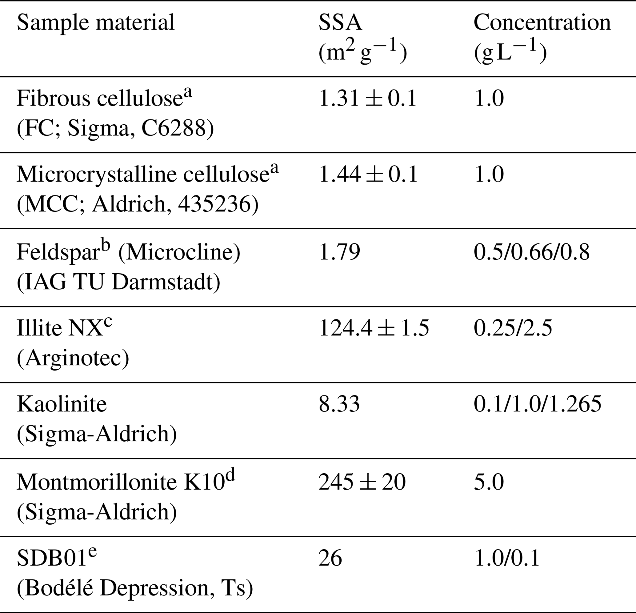
^a Same as used in Hiranuma et al. (2018). ^b Same as FS01 in Peckhaus et al. (2016). ^c Same as in Diehl et al. (2014) and Hiranuma et al. (2015). ^d Same as in Diehl et al. (2014). ^e Same as in Ullrich et al. (2019).

Atmospherically relevant INPs exhibit an extremely wide range in their heterogeneous-freezing ability. Furthermore, there is a large spread in the specific surface area (SSA) of the investigated materials from around 1 to 245 m² g⁻¹ (see Table 1). We therefore chose diverse mass concentrations for each of the different particle types to obtain reasonable numbers of freezing events within the temperature ranges of our measurement facilities. Furthermore, since the volume of the investigated droplets in the M-AL was approximately 20 times larger than in the M-WT, we used reduced mass concentrations in the M-WT to obtain overlapping freezing curves with the two methods (see Eq. 5).

Prior to each set of experiments, 20 to 40 mL aqueous suspension was prepared by mixing sample particles of known weight (measured by an analytical balance from Sartorius) with high-purity water (CHROMASOLV water for high-precision liquid chromatography, HPLC, Sigma-Aldrich). Between the measurement runs the aqueous suspension was continuously stirred at a very low rate using a magnetic stirrer to avoid coagulation and sedimentation of the particles in the suspension. A hypodermic syringe was used to inject suspension droplets into the measuring instruments. For the M-AL measurements, the syringe was filled with aqueous suspension after an idle time of about 30 min without stirring (following the sample preparation protocol of Hiranuma et al., 2019) so that at the uppermost part of the solution a homogeneous suspension was generated. For the M-WT measurements we abandoned an idle time because in this case we could presume already-homogeneous suspension due to the low particle concentration. Furthermore, the syringe was shaken prior to droplet injection in both M-AL and M-WT experiments to homogenize the particle distribution in droplets. Otherwise no pre-treatment procedures were applied.

Although efforts were made to unify and standardize the sample generation, we cannot rule out INP surface area variation among the investigated droplets. There are several sources of uncertainty in total surface area inside droplets like inhomogeneous distribution of particles among injected droplets, externally or internally mixed particles, aggregation due to sedimentation, and internal circulation. The most appropriate way to determine the actual INP surface area would be the continuous measurement of the surface area inside each droplet under investigation, but that seems not feasible currently. Another possibility is the measurement using size-selected particles, as in the study of Hartmann et al. (2016). Neglecting the variability in composition and surface area of INPs may introduce significant error in calculated n_s(T) and J_s(T) (Barahona, 2020). Furthermore, the assumption of identical INP surface area in each droplet imposes a cooling rate and surface area dependence on J_s(T) (Alpert and Knopf, 2016; Knopf et al., 2020). In our analysis we considered the error sources in concentration determination, in SSA, and in droplet size for determining the propagated error for the calculated parameters.

3.2 Experimental setups and procedures

The characteristics and deliverables of the M-WT and M-AL instruments essential for the present study are summarized in Table 2 and are described in the following subsections. Detailed descriptions of the experimental facilities are given, e.g., in Szakáll et al. (2010) and Diehl et al. (2011, 2014).

Table 2 Characteristics of the experiments conducted with the M-WT and M-AL.

3.2.1 M-WT (Mainz vertical wind tunnel)

The Mainz vertical wind tunnel (M-WT) is a worldwide unique experimental facility designated for the laboratory investigation of atmospheric hydrometeors, such as cloud droplets, raindrops, graupel, hailstones, and snowflakes. Single hydrometeors are floated freely at their terminal velocities in the laminar vertical updraft of the wind tunnel. Hence, the relevant physical properties of the hydrometeors, such as Reynolds numbers and ventilation coefficients, are equal to their values in the real atmosphere (Szakáll et al., 2010; Diehl et al., 2011).

For the immersion freezing experiments, the air in the M-WT was cooled down and kept constant (within ±0.3 ^∘C) at various temperatures between −15 and −30 ^∘C. For appropriate measurement statistics, at each temperature, particle type, and INP concentration, a total number of 70 aqueous-suspension droplets were investigated. After injection, each droplet was floated in the M-WT until it froze or until the experiment was terminated because of reaching a predefined time limit. The onset of freezing is characterized as a sudden significant change in floating behavior of the droplet caused by the irregular shape of the frozen particle. This changing behavior was visually observed and registered by the operator during the experiments. In this way, the total observation time, i.e., the time duration from injection until the onset of freezing, was recorded (Diehl et al., 2014). When a droplet did not freeze within 35 s, it was counted as unfrozen. In our earlier immersion freezing studies, we levitated the supercooled droplets for at most 30 s (if freezing was not initiated sooner), in accord with Eq. (15). We extended this total observation time by 5 s to consider the approximate time period a drop needed to approach its equilibrium temperature in the M-WT (Fig. 2). Furthermore, wind speed, air temperature, and dew point temperature (typically in a range from −20 to −35 ^∘C) in the wind tunnel were recorded continuously at 2 Hz temporal resolution.

The drop surface temperature was calculated using Eq. (B21) considering thermal-steady-state conditions between the levitating drop and its surrounding air. The time needed to approach the equilibrium temperature in the M-WT experiments within 0.2 K difference (i.e., below the temperature measurement precision of the applied PT100 sensor) was calculated at distinct M-WT air temperatures and plotted in Fig. 2 for different dew points. In the calculations the starting drop temperature was set to 20 ^∘C. One can observe a slight dependence of the adaptation time on the air temperature, but T_e was typically reached within 5 to 6 s for air temperatures between −15 and −28 ^∘C. In the calculations, dew points of −30, −27.5, and −25 ^∘C were applied, and the results are merged in the plot shown in Fig. 2. Hence, the adaptation time was found to be practically independent of the dew point for the M-WT experiments.

Figure 2 Time needed to approach the equilibrium temperature T_e with an accuracy of 0.2 ^∘C as a function of air temperature T_∞. Calculations carried out for dew point temperatures −30, −27.5, and −25 ^∘C are plotted by black, red, and blue dots, respectively. The data points were calculated using Eq. (B21). The regression line is $t_{\mathrm{a}}=\mathrm{3.46}-\mathrm{0.09}{T}_{\mathrm{\infty }}$ (T_∞ in ^∘C).

Typical droplet diameters were approximately 700 µm, corresponding to volumes around 0.18 µL. The size of each investigated droplet was determined from its terminal velocity (Beard, 1976), i.e., from the vertical air speed needed for freely suspending it, which can be measured with high accuracy in the M-WT (Diehl et al., 2014).

Immersion freezing in M-WT experiments was investigated under isothermal measurement conditions; hence, the stochastic approach was applied first for data analysis. Thus, the rate constant R and the nucleation rate coefficient J_het were calculated from Eqs. (2) and (3), respectively, using the number of freezing events as a function of the freezing time. In the analysis the freezing time of each droplet was calculated by subtracting the adaptation time (Fig. 2) from the total observation time lasting from droplet injection until the onset of freezing. Furthermore, from the number of freezing events over the whole observation time period, the frozen fraction f_ice(T) and the INAS density n_s(T) (Eq. 5) were determined by employing the singular approach by equating R⋅t to n_s.

Background measurements were carried out before each experimental run by floating at least 10 HPLC (high-precision liquid chromatography) water droplets for 35 s in the tunnel. We have not observed any freezing event during these test measurements, which indicates the absence of impurities (i.e., background active INPs) in both the HPLC water droplets and the wind tunnel.

3.2.2 M-AL (Mainz acoustic levitator)

The main component of the M-AL measurement facility is an acoustic levitator (APOS BA 10, tec5 GmbH), in which contact-free single-droplet levitation is maintained by a standing ultrasonic wave (Diehl et al., 2014). The M-AL is placed inside a walk-in cold room, where the ambient temperature was set to be −30 ^∘C for the freezing experiments. In order to prevent any disturbing air motion, which might cause unsteady temperature condition and unstable levitation or carry ice-nucleating particles onto the levitating drop surface, the M-AL was surrounded by a protective acrylic housing. Using this setup, the air temperature in the M-AL was −28 ^∘C, as measured by a PT100 sensor. An infrared thermometer (KT 19.82 II, Heitronics) and a digital video camera (USB-CAM-103H, Phytek GmbH) were arranged around the acrylic housing of the levitator.

One of the main advantages of the experimental setup of the M-AL is the direct observation of the surface temperature of the levitated drops during the cooling–freezing process, which was performed by the infrared thermometer at a rate of 2 Hz. The minimum observable spot size of the infrared thermometer restricted the minimum levitated-drop diameter to 2 mm. The actual drop size was determined from the images captured by the digital video camera instantaneously after injecting the drop into the M-AL. An example of a video recorded during an experiment on the ice nucleation ability of cellulose is provided as a video supplement of this paper (see https://doi.org/10.5446/46729, Szakáll and Mayer, 2020). In the video, the air temperature in the cold room measured by a PT-100 sensor, the continuously determined drop size (as the volume-equivalent diameter), and the drop surface temperature measured by the infrared thermometer are displayed. The recorded drop cools continuously, adapting its temperature to the ambient temperature until the freezing is initiated at about −21.8 ^∘C. The onset of freezing can be observed by the sudden change in the transparency of the droplet and the increase in the drop surface temperature to 0 ^∘C.

In case of M-AL experiments, the droplet surface temperature approached the equilibrium temperature in a slower manner than in the M-WT, which was primarily due to the larger drop size and smaller ventilation effect stemming from the acoustic field (see Appendix B3). The relatively moderate cooling and large drop surface area enabled us to determine the freezing temperature of the individual drops with high accuracy by the infrared thermometer. In Fig. 3 two typical examples of M-AL measurements are plotted: in one case (black line) no freezing occurred, and the experiment was terminated after 80 s measurement time. In the other case (red line), freezing was initiated after 35.5 s cooling, at about −21.3 ^∘C surface temperature. The arithmetic mean of the three recorded temperatures preceding the deepest drop surface temperature during the last 1.5 s before the onset of freezing, i.e., the temperature in transition from stage 1 to stage 2 in Fig. 1, was considered to be the freezing temperature. The number of frozen droplets was measured and binned in 1 K intervals to calculate f_ice and thereby n_s by applying the singular approach (Eq. 5).

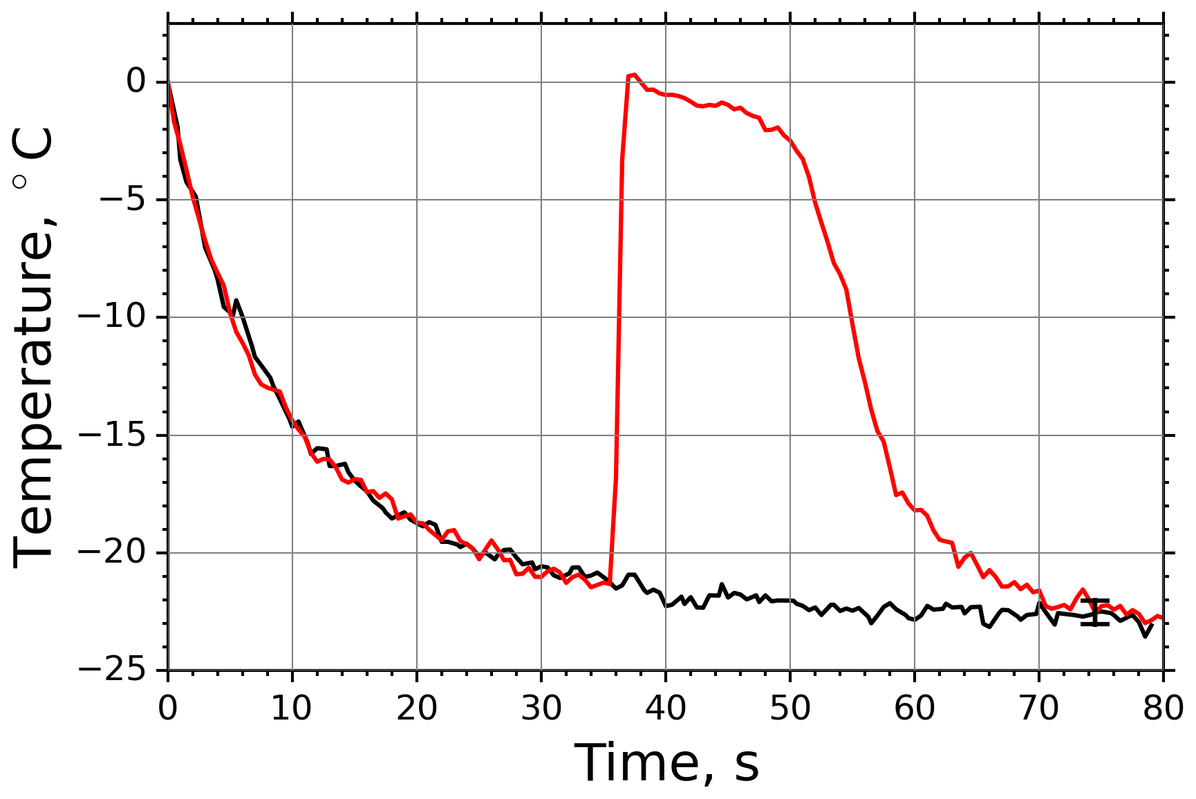
Figure 3 Measured surface temperatures of two droplets levitated in the M-AL: examples of freezing (red line) and non-freezing (black line) events. The measurement uncertainty in the temperature was ±0.5 K.

The temporal evolution of the drop temperature in the sample experimental run of the M-AL depicted in Fig. 3 can be described by the exponential-decay function Eq. (B16) with τ=11.3 s, applying a ventilation coefficient of 5.6, which is in accord with the findings of Lierke (1995). The relaxation time τ was determined for each experimental run in the M-AL and showed typical values between 8.94 and 15.42 s.

The actual cooling rate at a time instant during temperature adaptation is defined as $r\left(t\right)=-\mathrm{d}T/\mathrm{d}t$, which can be calculated after rearranging Eq. (18) to

$$\begin{array}{}\text{(19)}& T_{\mathrm{a}}=T_{\mathrm{e}}-\left(T_{\mathrm{e}}-T_{\mathrm{a}}(t=\mathrm{0})\right)\exp \left(-t/\mathit{\tau }\right).\end{array}$$

After some manipulation the actual cooling rate can be written as

$$\begin{array}{}\text{(20)}& r\left(T_{\mathrm{a}}\right)={\displaystyle \frac{T_{\mathrm{a}}-T_{\mathrm{e}}}{\mathit{\tau }}}.\end{array}$$

The r(T_a) curve for τ=11.3 s is shown in Fig. 4. It is apparent from the figure that at high temperatures the cooling rate is substantially high and gets moderate values only at low temperatures close to the equilibrium temperature. For such large cooling rates in M-AL measurements, Eq. (13) predicts a significant shift in drop freezing temperature.

Figure 4 Actual cooling rate as a function of temperature in the M-AL for the example shown in Fig. 3, with τ=11.3 s.

4 Results and discussion

In this section we present the results of M-WT and M-AL experiments on immersion freezing using the clay mineral kaolinite. The data for other materials listed in Table 1 are presented in Appendix A.

4.1 M-WT experimental results

Figure 5 shows the INAS densities computed using Eq. (5) from f_ice spectra obtained from M-WT measurements of kaolinite with concentrations of 0.1 and 1.0 g L⁻¹, marked with light- and dark-blue symbols, respectively. The number of data points is limited to five, which is the issue of the M-WT experiments being very laborious for collecting statistically relevant numbers of measurements for each temperature. Comparing Fig. 5 with the INAS densities of other investigated materials presented in Appendix A reveals that kaolinite is a good atmospheric INP, exhibiting large n_s values that, nevertheless, vary steeply over 1 order of magnitude within the investigated temperature range of only 4 K, i.e., here from 252 to 256 K.

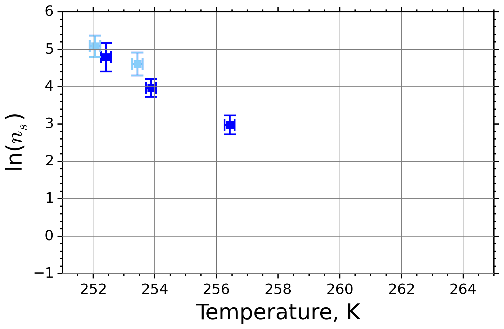
Figure 5 INAS density for kaolinite as a function of temperature determined from the frozen fraction of 0.1 and 1.0 g L⁻¹ suspension drops (marked with light and dark blue, respectively) investigated in the M-WT. Each data point represents 70 individually measured droplets, each of which with diameter of approximately 700 µm. The error bars represent the 1σ values of the measured air temperatures and the calculated drop sizes.

Figure 6 Kaolinite: (a) the decrease in fraction of droplets which remained liquid with time at different temperatures in the isothermal experiments in the M-WT. The colors correspond to different temperatures; experiments with particle concentrations of 0.1 and 1 g L⁻¹ are plotted by triangles and rectangles, respectively. The gray symbol marks a data point for 1 g L⁻¹ at 253.9 K and indicates typical error bars. (b) Freezing rate of kaolinite normalized to surface area as a function of temperature calculated from (a) using Eq. (21). The horizontal error bars are the 1σ values of the measured temperatures, while the vertical error bars represent the fit error in $R/A$ calculation.

For computing n_s for Fig. 5 using Eq. (5), the fraction of frozen droplets f_ice was determined by employing the singular approach, i.e., by counting the number of droplets frozen in an experimental run, disregarding the time from injection until freezing. A droplet remaining liquid for up to 35 s (i.e., the end of the experimental run) was classified as unfrozen.

From the time-resolved measurement data from the M-WT, the time dependence of the freezing process was analyzed. For that, Eq. (2) was rearranged to

$$\begin{array}{}\text{(21)}& \ln \left({\displaystyle \frac{n_{\mathrm{liq}}(T,t)}{N_{\mathrm{tot}}}}\right)=-R\left(T\right)\cdot t,\end{array}$$

where $n_{\mathrm{liq}}(T,t)=\mathrm{1}-n_{\mathrm{fr}}(T,t)$ is the number of droplets remaining liquid after time t at temperature T. Figure 6 depicts the time dependence of liquid ratio from the M-WT measurements at five different temperatures and using the two distinct concentrations of kaolinite as for Fig. 5. The times needed for the injected droplets to reach their equilibrium temperatures (i.e., 6 s; see Fig. 2) were subtracted from the recorded time interval between injection and freezing. At lower temperatures and with higher particle surface areas per drop (i.e., higher INP concentration), the curves get steeper, indicating that freezing proceeds faster. Figure 6a clearly shows the expected exponential decay of liquid drops predicted by the stochastic approach. The temperature dependence of the normalized freezing rate according to Eq. (21) as shown in Fig. 6b was determined by computing the slopes of the curves in Fig. 6a and dividing them by the total surface areas of INPs immersed in the examined water droplets. Figure 6b reveals the expected linear dependency of $R/A$ in agreement with Eq. (10). Hence, ω, which is the slope of $R/A$ (see Eq. 10), can readily be determined for the investigated kaolinite sample from Fig. 6b by linear regression as $\mathit{\omega }=\mathrm{0.49}\pm \mathrm{0.03}$. (Here the error in ω is the standard error in the linear fit.) Note that if the INPs can be considered to be single-component, then $J_{\mathrm{s}}=R/A$. In our experiments, the total surface area A was estimated from the concentration of the aqueous solution and from the specific surface area. Accurately measuring the actual total surface area of INPs inside the droplets, which should be taken into account for calculating ω and J_s, is currently not feasible. Therefore, the error in A might be significantly higher than estimated, which would result in a false classification of the INPs as single-component.

4.2 M-AL experimental results

Frozen fractions of kaolinite suspension with 1.265 g L⁻¹ concentration as a function of temperature are shown in Fig. 7a. Error bars are associated with the temperature bin interval (±0.5 K), and the uncertainty in the determination of f_ice stems from the counting statistics and the experimental temperature uncertainty. The active-site density n_s calculated from Eq. (5) using f_ice in Fig. 7a is plotted in Fig. 7b. Here the error bars originate from Gaussian error propagation when using the measured data in Fig. 7a. From the calculation we excluded the data points for which f_ice was above 90 % or below 10 %. This cutoff was introduced because in these cases the uncertainty in f_ice was very large due to the poor counting statistics when freezing or unfreezing events occur very rarely.

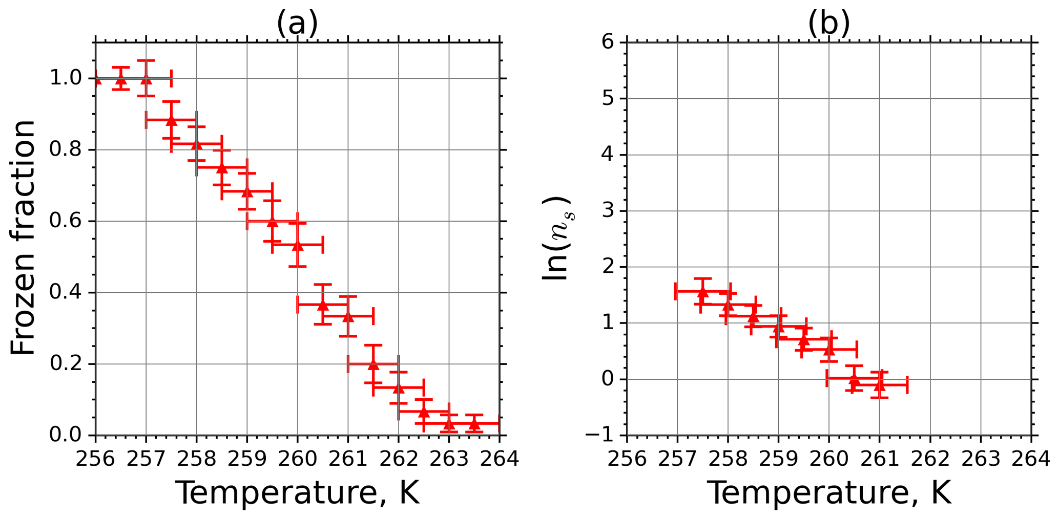
Figure 7 (a) Frozen fraction of 2 mm aqueous-suspension droplets containing 1.265 g L⁻¹ kaolinite measured in the M-AL. (b) INAS density of kaolinite as a function of temperature determined from the spectrum shown in (a).

Another criterion for using f_ice for further evaluations was that it should significantly exceed the background nucleation caused by impurities in the water used for generating the aqueous suspension. To determine this background spectrum, we investigated pure water droplets before each experimental run in the M-AL, similarly to the M-WT measurements. However, in contrast to the findings for the M-WT, some of the HPLC water droplets froze in the M-AL. This indicates that the abundance of impurities in the HPLC water was high enough in the relatively large (∼4 µL) drops in the M-AL to initiate freezing. Therefore, f_ice spectra for pure water samples were measured in a similar way as for the INPs (Fig. 8). Although the number of freezing droplets was relatively small at temperatures higher than 248 K, in some cases (e.g., when low concentrations were used) the INP nucleus spectra had to be corrected by considering the water background spectrum as described below.

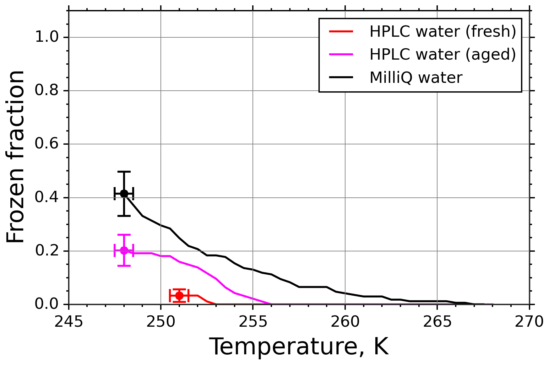
Figure 8 Freezing spectra of water of different purity grades: high-precision liquid chromatography water (HPLC; Sigma-Aldrich) and in-house-purified Milli-Q water.

In earlier experiments in the M-AL (e.g., Diehl et al., 2014), in-house-produced Milli-Q water was used as a solvent for the aqueous solutions. Therefore, we also analyzed the Milli-Q water in our present experiments. The results are plotted by black symbols in Fig. 8. Apparently, using HPLC water from a freshly opened chemical bottle (red symbols) reduces the background f_ice. Nevertheless, the f_ice spectrum of HPLC water changed with time and increased significantly after about a year (magenta symbols), indicating an aging effect. This behavior of different water types is in accord with the finding of Hiranuma et al. (2019). Since it is difficult to eliminate the contribution of INPs still present in high-purity water (see Fig. 8, and Whale et al., 2015), we applied a background correction method described below using the f_ice spectrum for pure water drops collected prior and during each set of experiments.

The background spectra were also corrected by shifting the freezing temperature following Vali (2014) with

$$\begin{array}{}\text{(22)}& \mathit{\beta }=\mathrm{0.66}\lg \left(r\right).\end{array}$$

Although Vali proposed the factor of 0.66 for the temperature correction of pure water, this parameter depends most probably on the type of impurities in the water. This is also suggested by Fig. 8 since the frozen-fraction spectra are significantly different for different water samples, purity grades, and water age. Nevertheless, the temperature correction of Eq. (22) barely shifts the background spectra: β=0.46 for 252 K, where the cooling rate in the M-AL is approximately 252 K min⁻¹. Such a temperature shift would increase the background frozen fraction by less than 0.05. Therefore, no background subtraction (as, e.g., in Hader et al., 2014) was applied, but a cutoff temperature was defined where the difference between the background and the INP spectra was less than 0.05. This correction method was only necessary for FC and MCC in our experiments, while the other materials initiated freezing at higher temperatures for the investigated concentrations.

5 Reconciling the M-WT and M-AL experimental data by temperature correction

Plotting the INAS densities obtained from M-WT and M-AL experiments, respectively, in one figure reveals an apparent shift in the curves in either ln (n_s) or in the temperature (Fig. 9a). This shift was found for all investigated materials but with different magnitudes (see Appendix A). Curves of INASs as a function of temperature from the same experimental methods (M-AL or M-WT) but measuring different INP concentrations (see Table 1) do not spread in such a systematic way, which indicates that the shift stems very likely from the detected freezing temperatures. Since the M-AL exhibits a very large cooling rate for temperatures higher than 255 K (see Fig. 4), a temperature shift predicted by Eq. (13) can be significant for some given materials depending on their λ values. Nevertheless, we thoroughly checked other possible sources of any systematic freezing-temperature shift. One obvious issue might arise from the relatively large volume of the drops examined in the M-AL. In the experiments the surface temperature of the drops was continuously measured; however, if the drop cools down at a high rate, heat from the drop interior might not be transported outward sufficiently quickly. Some INPs are located inside the drop, i.e., away from the drop surface; hence, they would experience higher temperatures than measured by the IR thermometer. This might falsify the experimentally determined temperature dependence of the ice-nucleating ability. Nevertheless, our computation of the temporal evolution of a continuously cooling drop showed a maximum temperature difference of 0.5 K between the drop interior and surface, which is within the measurement error in the M-AL (see Appendix B4). This temperature difference is higher at higher temperatures, where fewer freezing measurements were carried out. At surface temperatures below 258 K, the difference is only about 0.2 K. Furthermore, the number of kaolinite particles in a 0.1 g L⁻¹ aqueous-suspension drop of 2 mm diameter, for instance, is approximately 300 000. Thus, numerous particles will occur in the coldest region of the drop. Since a single particle is sufficient to initiate nucleation, the warmer temperature in the drop interior plays a minor role in initiating the freezing.

Figure 9 (a) Composite INAS density spectrum of kaolinite from the uncorrected M-WT (blue) and M-AL (red) measurements. Panels (b) and (c) show the temperature-corrected data points from the M-WT and M-AL experiments based on λ and ω, respectively. The dash-dotted line in (c) is the regression line for the corrected data points obtained by employing the optimal λ value as in (b).

To modify the measurement data according to the temperature shift due to cooling rate and interparticle variability in ice nucleation efficiency, we follow the approach of Herbert et al. (2014) as described in Sect. 2. We present here only the case of kaolinite as an example; the approach was applied to reconcile the data for all examined materials. Those results are presented in Appendix A. The procedure for modifying for the raw data set in the M-AL and M-WT is depicted as a flow diagram in Fig. B5.

Determination of λ

The parameter λ for the temperature shift was determined assuming that with the correct λ value, the ln (n_s) data from the two M-WT and M-AL experiments converge onto one single curve. Therefore, the temperatures of the unmodified data were shifted by applying Eq. (11) to the isothermal experimental data from the M-WT and Eq. (13) to the data obtained using the continuous-cooling approach of the M-AL. For each investigated INP species a set of λ values varying from 0.1 to 8.0 in 0.1 steps applied for the modification in Eqs. (14) and (13). A linear fit to the derived ln (n_s) (solid black line and black data points in Fig. 10a) and the RMSE (root mean square error) between the data and the linear fit were calculated for each set of modified experimental data. The RMSE for the set of λ values for the kaolinite experiments is depicted in Fig. 10b. The optimal λ value, 1.7 in the present case, corresponds to the minimum of the RMSE curve. This optimal value provides the best linear fit among the tested λ values.

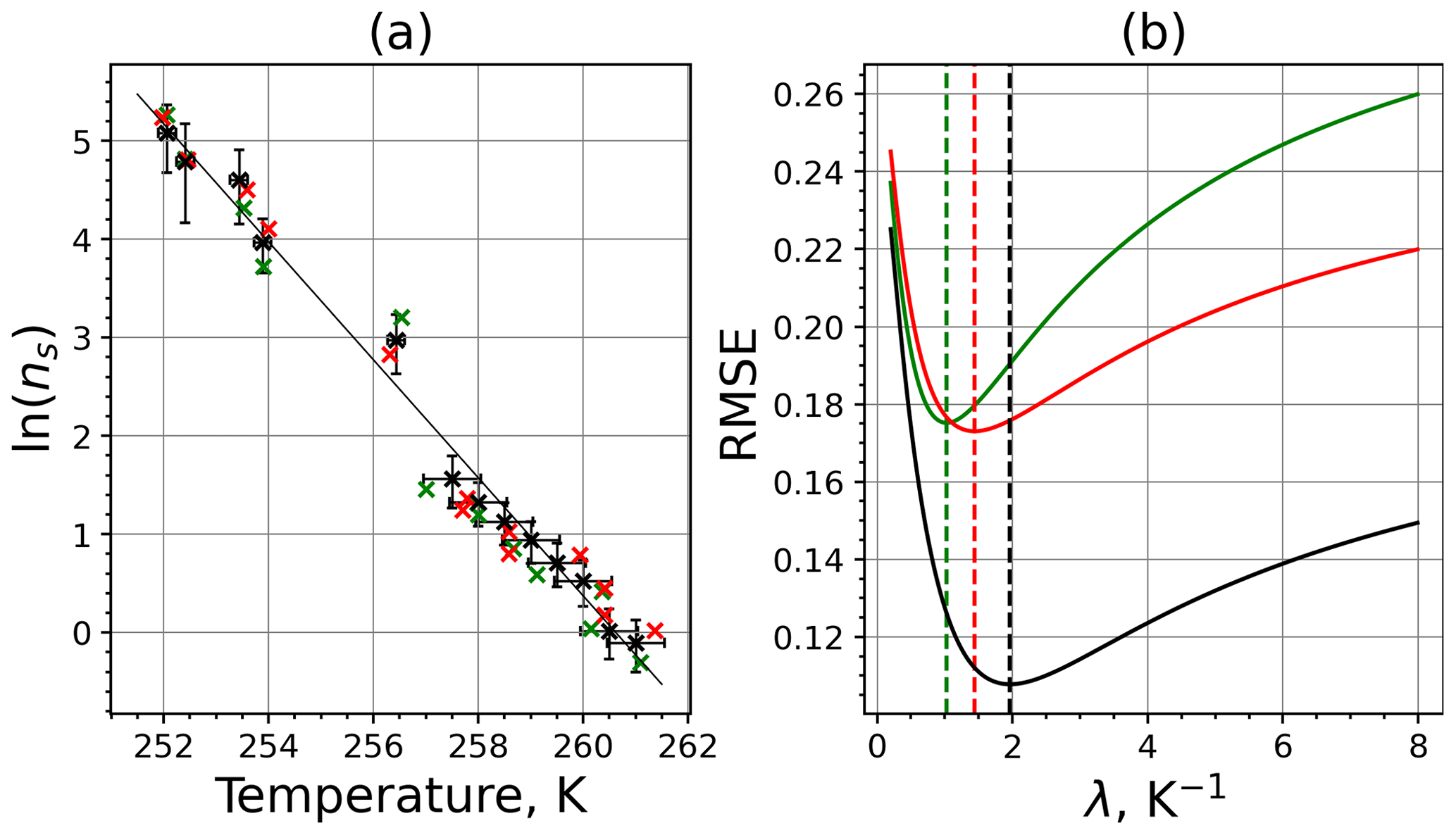
Figure 10 (a) Original (black; same as in Fig. 9a) data set and two data sets randomly generated within the experimental error interval (red and green) using the measured INAS densities of kaolinite. The solid black line is the linear fit to the original experimental data set. (b) RMSE as a function of lambda for 2 of the 1000 randomly generated data sets. The dashed vertical lines indicate the optimal lambda values for the red, green, and black curves.

To determine the error in λ originating from the measurement error, the following procedure was used. We generated random data around each of the actually calculated n_s data points but within the bounds of the measurement error (assuming the error bar of the measurement corresponding to 1σ). Hence, the number of data points for the λ analysis did not change, but each data point was shifted in both temperature and n_s. Here, the distribution of n_s and T was not considered; random values within the error bounds were taken. Then, the optimal λ value for this modified data set was determined. We repeated this procedure 1000 times by generating new random data points, and from the statistical analysis of the obtained λ values, Δλ was calculated. Choosing random values within the 1σ bounds around the mean data and neglecting values outside this bound might result in overestimating Δλ. As an example for the procedure, two randomly generated data sets (plotted in red and green colors) and the corresponding RMSE values as a function of λ are shown in Fig. 10a and b, respectively.

The optimal λ value of 1.7 was used to apply the temperature shift caused by the residence time dependency of the freezing process in the M-WT and by the cooling rate dependency in the M-AL. The modified data points together with the fitted regression line are plotted in Fig. 9b. When comparing Fig. 9b to Fig. 9a, the agreement between the modified data points from the two distinct experimental methods is apparent. This is also supported by the high R² value of the regression line.

The temperature gradient of the normalized freezing rate, ω, is determined in Sect. 4.1 from the time dependency of the frozen fraction measured in the M-WT. The data points modified by the temperature shift Eq. (13) presuming ω=λ are plotted in Fig. 9c together with the best-fit line. Again, an obvious agreement can be seen between the two distinct experimental methods.

For a single-component INP, ω is equal to λ, which was found in Herbert et al. (2014) for their kaolinite sample from the Clay Mineral Society. In our study the ω=0.49 and λ=1.7 values for our kaolinite sample from Sigma-Aldrich differ. The deviation in the temperature correction based on λ and ω is further emphasized in Fig. 9c, where the regression lines obtained by employing the optimal λ values and ω are plotted by dash-dotted and dashed lines, respectively. This plot suggests that the kaolinite sample investigated in our study has to be treated as a multi-component system, and the determined λ value should be employed for modifying the measured freezing temperatures.

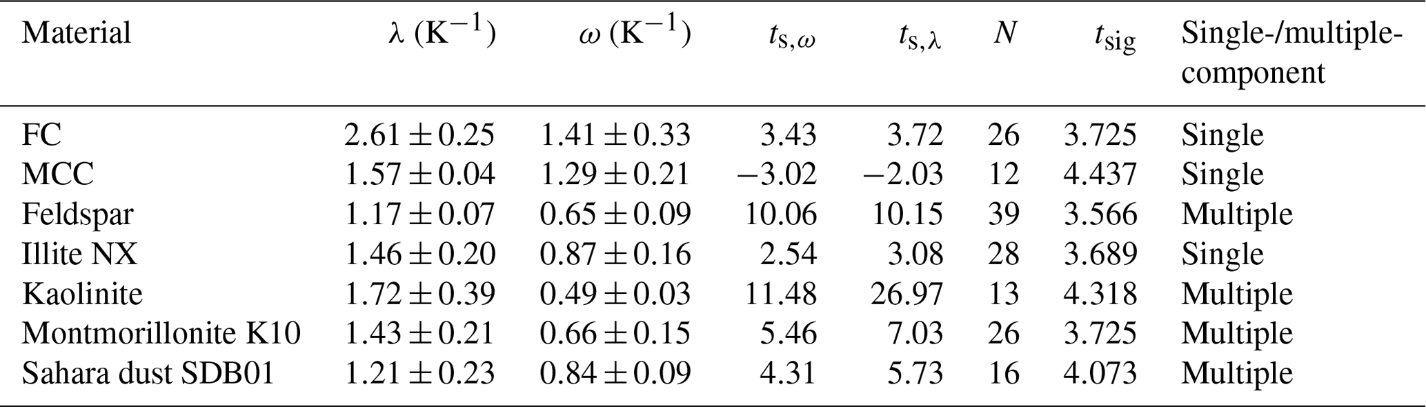
The ω and λ values for the investigated materials are listed in Table 3. After the definition of Vali (1994) and Herbert et al. (2014), all materials exhibit multiple-component behavior since ω<λ in all cases. Nevertheless, for some materials, e.g., illite NX, despite different λ and ω values the deviation between the data sets modified using λ or ω was not obvious (see Appendix A). To obtain further insights into this feature, we performed statistical-significance tests as follows.

Table 3 λ and ω values and the classification of the investigated materials. The results of statistical t tests are also given: calculated t values, number of samples (data points), and t values showing significance in α=99.5 %.

First, we computed the arithmetic-mean curve of the two best-fit lines corresponding to λ and ω, respectively, and calculated their mean deviation $\stackrel{\mathrm{‾}}{d}$ from that mean curve. The ultimate question of our statistics tests was whether the mean deviation is significant with respect to the measurement error and data scatter. Hence, as the next step, the error-weighted standard deviations of the residuals s_ω and s_λ were calculated as

$$\begin{array}{}\text{(23)}& {\displaystyle }{s}_{\mathit{\omega }}=\sqrt{{\displaystyle \frac{{\sum }_{i=\mathrm{1}}^N\frac{{\left({\mathrm{\Delta }}_{\mathit{\omega },i}-\stackrel{\mathrm{‾}}{{\mathrm{\Delta }}_{\mathit{\omega }}}\right)}^{\mathrm{2}}}{\mathrm{\Delta }{T}_i^{\mathrm{2}}}}{{\sum }_{i=\mathrm{1}}^N\frac{\mathrm{1}}{\mathrm{\Delta }{T}_i^{\mathrm{2}}}}}}\text{(24)}& {\displaystyle }{s}_{\mathit{\lambda }}=\sqrt{{\displaystyle \frac{{\sum }_{i=\mathrm{1}}^N\frac{{\left({\mathrm{\Delta }}_{\mathit{\lambda },i}-\stackrel{\mathrm{‾}}{{\mathrm{\Delta }}_{\mathit{\lambda }}}\right)}^{\mathrm{2}}}{\mathrm{\Delta }{T}_i^{\mathrm{2}}}}{{\sum }_{i=\mathrm{1}}^N\frac{\mathrm{1}}{\mathrm{\Delta }{T}_i^{\mathrm{2}}}}}},\end{array}$$

where ΔT_i is the temperature measurement error, Δ_ω,i and Δ_λ,i are the deviations of the corrected data points from the corresponding best-fit curves, and $\stackrel{\mathrm{‾}}{{\mathrm{\Delta }}_{\mathit{\omega }}}$ and $\stackrel{\mathrm{‾}}{{\mathrm{\Delta }}_{\mathit{\lambda }}}$ are the mean values of these deviations. For the significance test we applied a two-sided Student t test to a significance level of 99.9 % and calculated

$$\begin{array}{}\text{(25)}& {\displaystyle }{t}_{\mathrm{s},\mathit{\omega }}={\displaystyle \frac{|\stackrel{\mathrm{‾}}{d}-{\mathit{\mu }}_{\mathrm{0}}|}{s_{\mathit{\omega }}}}\cdot \sqrt{N}\text{(26)}& {\displaystyle }{t}_{\mathrm{s},\mathit{\lambda }}={\displaystyle \frac{|\stackrel{\mathrm{‾}}{d}-{\mathit{\mu }}_{\mathrm{0}}|}{s_{\mathit{\lambda }}}}\cdot \sqrt{N},\end{array}$$

where N is the number of data points. The null hypothesis was that the two linear curves do not significantly differ; thus, μ₀=0 for their deviation from the arithmetic-mean curve. In Table 3 we listed the calculated t_s,ω and t_s,λ, the number of data points, and the tabulated t_sig (β=99.9 %) values for the Student t test for each material. If t_s,ω or t_s,λ is greater than t_sig (β=99.9 %), then the null hypothesis is rejected. That means that the two best-fit lines differ significantly with respect to data scatter and measurement error, and consequently, the material is treated as multiple-component on a 99.9 % confidence level. Otherwise we consider the material to be single-component, although the statistical test does not prove the null hypothesis. Hence, we classify the material as single- or multiple-component within our measurement error and data scatter.

As listed in Table 3, according to our statistical test, kaolinite, feldspar, montmorillonite, and Sahara dust are multiple-component, while illite NX, FC, and MCC are single-component INPs. This implies that the definition of Herbert et al. (2014) to distinguish between single- and multiple-component samples on the basis of λ and ω values cannot directly be adapted to our M-AL and M-WT experiments. This is the consequence of the adaptive cooling of the drops in the M-AL, which results in a temperature dependence on the λ-based correction. Thus, the same λ value caused a higher temperature correction at higher temperatures (see Fig. B4 in Appendix B). Therefore, our analysis indicates that statistic tests have to be performed considering both data scatter and measurement error to compare the λ and ω values. This procedure improves the classification of the materials as single- or multiple-component.

The statistical tests supported the finding that the kaolinite that we analyzed is multiple-component. That contradicts the finding of Herbert et al. (2014), who showed their kaolinite sample (KGa-1b from the Clay Mineral Society) to be single-component with $\mathit{\lambda }=\mathit{\omega }=\mathrm{1.12}$. This indicates that these two kaolinite samples are different, and thus the result outputs cannot directly be compared since the ice nucleation activity of materials depends on their specific chemical composition, which is known to be very variable for kaolinite. For example, the λ value for the kaolinite used in the cooling experiments of Wright and Petters (2013) was 1.7, which is equal to our result. In contrast, the Fluka kaolinite sample measured by Welti et al. (2012), which is known to contain particles of very-ice-active feldspar, had a λ value of 2.2 (see Table 2 in Herbert et al., 2014). In general, we found slightly higher λ values for biological aerosols (FC and MCC) than for mineral dusts. This results in smaller ΔT in Eq. (9), and hence, biological INPs show a weaker time dependence, in agreement with the findings of Peckhaus et al. (2016) and Budke and Koop (2015). For the investigated samples in our experiments, the temperature correction ranged from ≈0.5 K up to several kelvins, depending on the material's λ value (see also Fig. B4).

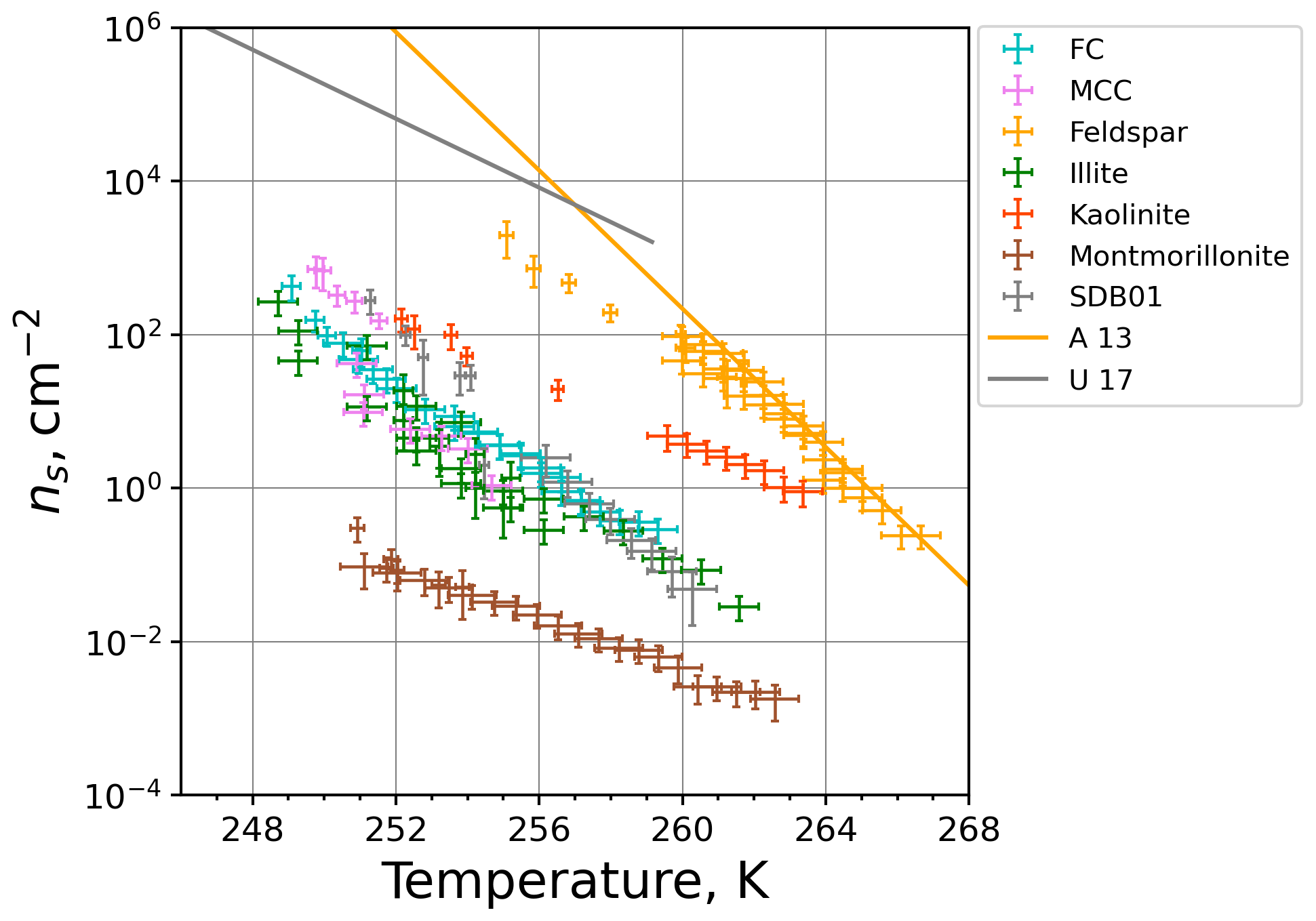
Figure 11 INAS densities of the investigated materials as a function of temperature. The data points are composites from M-WT and M-AL measurements and are corrected for the cooling rate. Orange and gray solid lines show parameterizations for feldspar (Atkinson et al., 2013) and desert dust (Ullrich et al., 2017), respectively.

The composite plot of the INAS densities for all investigated materials obtained by M-WT and M-AL measurements is shown in Fig. 11. In accord with the literature (e.g., Atkinson et al., 2013), feldspar is by far the most efficient ice-nucleating particle type among the investigated dust materials. Besides feldspar, kaolinite also has a high ice nucleation efficiency, in particular at higher temperatures. The biological particles (FC, MCC) and the clay minerals illite NX and Sahara dust have similar temperature-dependent n_s values. The one exception is montmorillonite, which was found to be the least efficient within the investigated temperature range from 248 to 266 K. Also shown in Fig. 11 are parameterizations for feldspar (Atkinson et al., 2013) and for desert dust (Ullrich et al., 2017). Our temperature-corrected feldspar data fit very well to the parameterization of Atkinson et al. (2013), which was based on cold-stage experiments, i.e.,  using aqueous suspensions of INP material. In contrast, the desert dust parameterization of Ullrich et al. (2017) is based on dry-deposition experiments and predicts higher INAS densities as measured in the M-WT and M-AL. This is in accord with the literature as for example Hiranuma et al. (2019) revealed different INAS densities when dry-deposition or aqueous-suspension techniques were utilized.

6 Conclusions and suggestions

Immersion freezing efficiencies of different types of aerosol particles such as pure and natural clay minerals as well as biological particles were studied using two distinct measurement techniques: an acoustic levitator (M-AL) and a vertical wind tunnel (M-WT). Both instruments utilize freely floating individual droplets.

The INAS densities of different types of aerosol particles obtained by the M-AL and M-WT revealed a shift in the freezing temperatures to lower values. Such a shift in freezing temperatures became obvious in our earlier experiments in the measurement campaigns FIN02 (DeMott et al., 2018) and INUIT (Hiranuma et al., 2019). Therefore, we had already corrected the data published in those papers for the freezing-temperature shift. Following the procedure depicted in Fig. B5, we were able to bring the INAS densities obtained from the two different methods in line. We have also reconciled our earlier experiments on illite NX (Diehl et al., 2014) and ascertained that those data were burdened with a temperature shift as well. A modification of the data in Diehl et al. (2014) according to our new findings further improves the agreement of the data from the M-WT and M-AL (green symbols in Fig. 11).

Taking advantage of having two independent single-droplet levitation methods located in our laboratory, we determined the material-dependent λ value, which determines the temperature shift due to cooling rate for the investigated aerosol types based on the analysis method suggested by Herbert et al. (2014). Furthermore, we classified the aerosol materials investigated in this study as single- or multiple-component, i.e., whether their nucleation process shows weak or strong time dependence. This result has a direct impact on the applicability of the singular approach to the evaluation of data from immersion freezing with various INP types, i.e., whether the time dependence of freezing can be neglected or not. Further, if an INP type is single-component, the temperature shift can ultimately be calculated from the gradient of the measured freezing rate ω.

An important conclusion on the applicability of laboratory immersion freezing techniques can be made due to the different airflow conditions applied in our experiments. In the M-WT a continuous airflow is established around a floating droplet (correctly simulating real atmospheric conditions), whereas the M-AL maintains levitation with a very weak airflow. Since the INAS densities obtained by the M-WT and M-AL after applying the temperature shift due to the cooling rate show very good agreement, one can conclude that the airflow around the droplets containing the INPs does not significantly influence the immersion freezing process.

Based on the experiences collected during the presented synergetic study, we suggest the following points for future immersion freezing studies:

• If the instrument used for the measurements utilizes a continuously varying cooling rate, then its temperature adaptation decay first has to be characterized in terms of equilibrium temperature and decay constant and the corresponding uncertainties. Furthermore, the drop temperature has to be measured directly because it can significantly deviate from the ambient temperature.

• When comparing the ice nucleation efficiencies measured by different instruments utilizing distinct cooling rates, the comparison has to be carried out very carefully and critically. We suggest using the same or at least similar cooling rates in the different instruments in such intercomparison studies.

• We note from Fig. 8 that freezing behavior and, consequently, the necessity of background correction depend on the purity grade and age of water used for producing aqueous-suspension samples. Therefore, this water has to be carefully characterized for all experiments as well.

• In case the INAS densities are measured by applying a non-standard cooling rate (i.e., r≠1 K min⁻¹), the freezing temperatures have to be corrected following the procedures of Herbert et al. (2014) and the one described in this study. It has to be taken into account that the temperature shift is material-dependent and most probably temperature-dependent for most of the INPs.

• By the characterization of the aerosol material in terms of a temperature shift due to changes in the cooling rate, statistical-significance tests should be carried out taking both the data scatter and the measurement error into account. Of course, by increasing the measurement sensitivity (i.e., decreasing the measurement error) or by decreasing the data scatter (either by improving the measurement accuracy or due to a reduced natural variability in the sample material), the prediction of whether the ice nucleation of the material can be described using a single- or a multiple-component model will be more accurate. Nevertheless, the classification can only be obtained within the measurement error and accuracy of the applied experimental method.

• In cloud models the cooling rate has to be considered, and the freezing temperatures of materials have to be corrected, taking the material-dependent λ values into account.

• It has to be emphasized that the total surface area of the particles in the individual droplets is a crucial parameter for the procedure described in this paper (see Eq. 5). It can vary, for instance, with sample particle size distribution or due to aggregation inside the droplets. It should be determined in each droplet under investigation, which seems currently not feasible. In our study we estimated the total surface area from the concentration of our aqueous solutions and from the specific surface areas of the materials. Alternatively, size-selected particles might be used for the immersion freezing measurements, which would decrease the surface area uncertainty (Alpert and Knopf, 2016) and improve the analysis conducted here. We also note that the model calculations of Alpert and Knopf (2016) concluded that the assumption of identical particle surface area in the droplets imposes a cooling rate dependence on J_s, which was not the case in our considerations. Based on these calculations, Knopf et al. (2020) demonstrated that surface area variance and stochasticity explain the freezing of illite NX. Furthermore, as demonstrated by Barahona (2020), composition and surface area variation between INPs may introduce biases in calculated n_s(T) and J_s(T), implying the necessity of the accurate determination of these quantities in laboratory immersion freezing experiments. The variability in particle surface area from droplet to droplet in our M-WT measurements might cause the non-linear behavior of $\ln (n_{\mathrm{liq}}/N_{\mathrm{tot}})$ for some INP materials (see Appendix A).

• The λ parameter and the temperature shifts in some aerosol species determined by Herbert et al. (2014) and in the present study serve rather for orientation. We suggest the determination of such temperature shifts for the specific material samples under investigation in each future experimental study on immersion freezing of aerosol particles. Variations in chemical composition, aging, sample contamination, and other parameters can result in changes in λ.

Appendix A: Further reconciled experimental results

In this section we provide the experimental results for the determination of the temperature-dependent freezing rate (as in Fig. 6) as well as the composite INAS density spectra from the M-WT and M-AL using λ and ω (as in Fig. 9) for the materials listed in Table 1.

A1 Fibrous cellulose (FC)

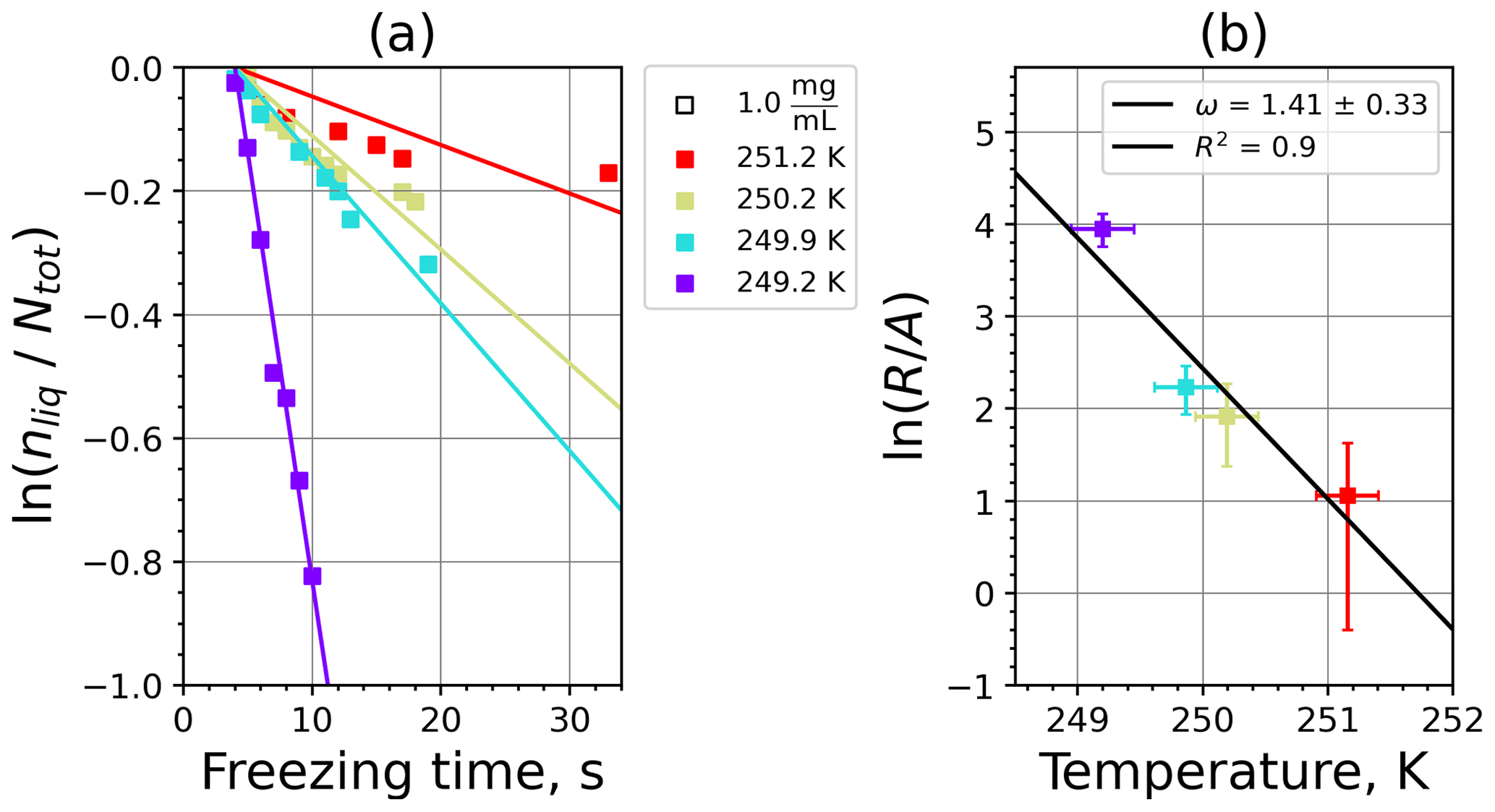
Figure A1 (a) The decrease in fraction of droplets which remained liquid with time at different temperatures in the isothermal experiments of fibrous cellulose (FC) at the M-WT. The colors correspond to different temperatures (particle concentrations of 1 g L⁻¹). Typical error bars are depicted in Fig. 6. (b) Freezing rate of FC normalized to surface area as a function of temperature.

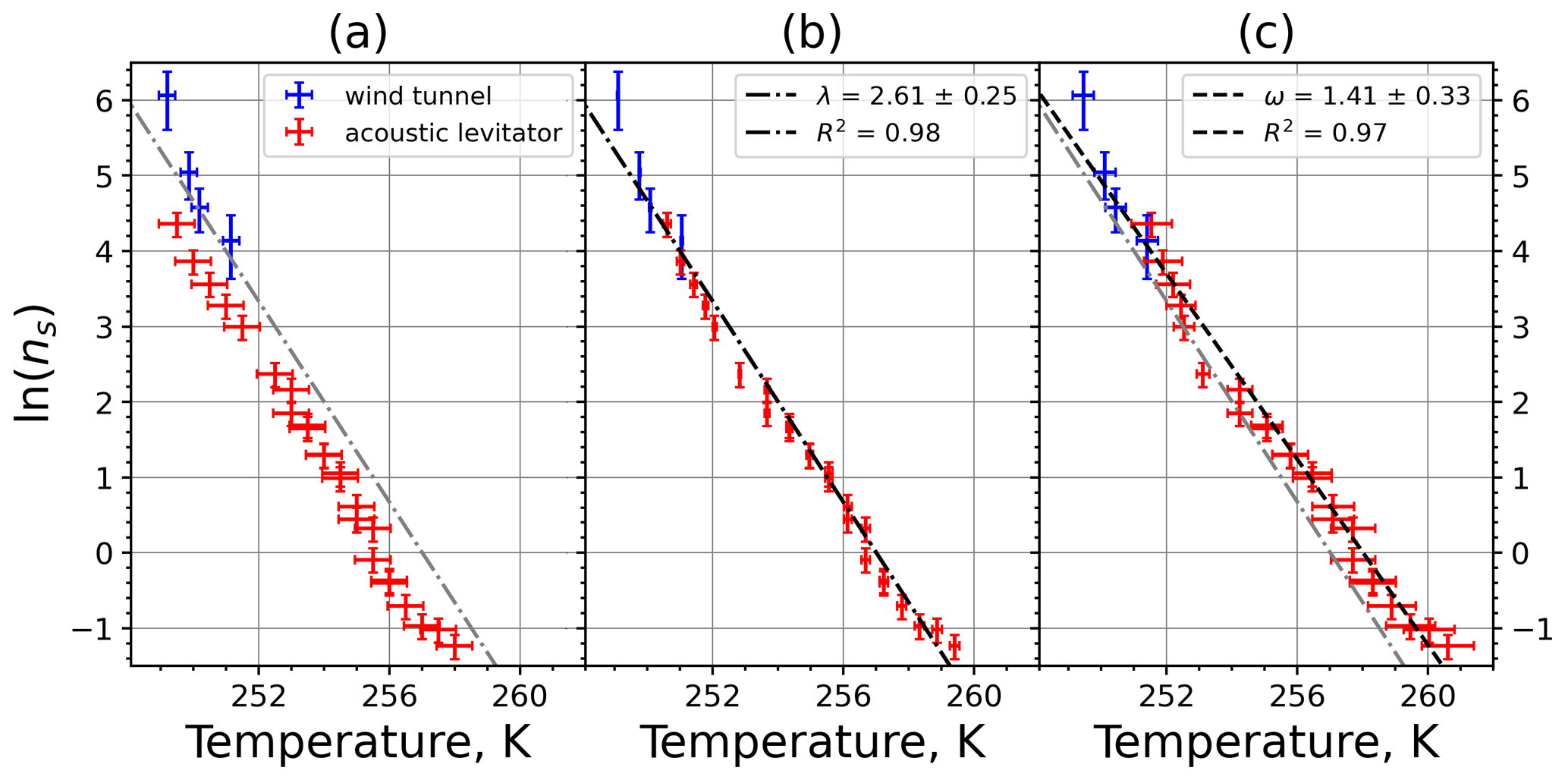
Figure A2 (a) Composite INAS density spectrum of FC from the uncorrected M-WT (blue) and M-AL (red) measurements. Panels (b) and (c) show the temperature-corrected data points from the M-WT and M-AL experiments based on λ and ω, respectively. The dash-dotted line in (c) is the regression line on corrected data points obtained by employing the optimal λ value as in (b).

A2 Microcrystalline cellulose (MMC)

Figure A3 (a) The decrease in fraction of droplets which remained liquid with time at different temperatures in the isothermal experiments of microcrystalline cellulose (MCC) at the M-WT. The colors correspond to different temperatures (particle concentrations of 1 g L⁻¹). Typical error bars are depicted in Fig. 6. (b) Freezing rate of MCC normalized to surface area as a function of temperature.

Figure A4 (a) Composite INAS density spectrum of MCC from the uncorrected M-WT (blue) and M-AL (red) measurements. Panels (b) and (c) show the temperature-corrected data points from the M-WT and M-AL experiments based on λ and ω, respectively. The dash-dotted line in (c) is the regression line on corrected data points obtained by employing the optimal λ value as in (b).

A3 Feldspar

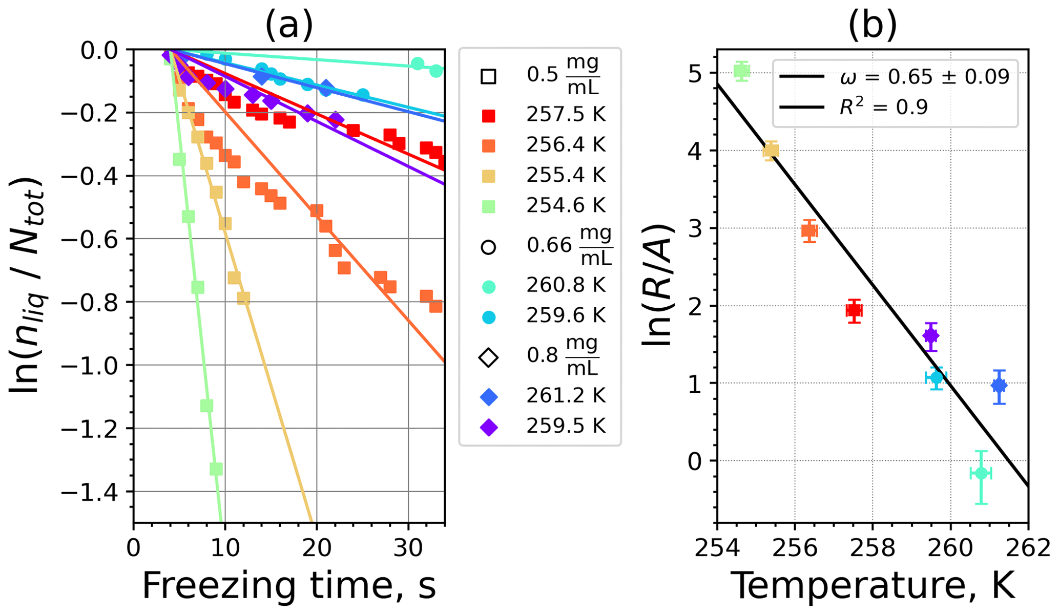
Figure A5 (a) The decrease in fraction of droplets which remained liquid with time at different temperatures in the isothermal experiments for feldspar at the M-WT. The colors correspond to different temperatures; experiments with particle concentrations of 0.5, 0.66, and 0.8 g L⁻¹ are plotted by rectangles, circles, and triangles, respectively. Typical error bars are depicted in Fig. 6. (b) Freezing rate of feldspar normalized to surface area as a function of temperature.

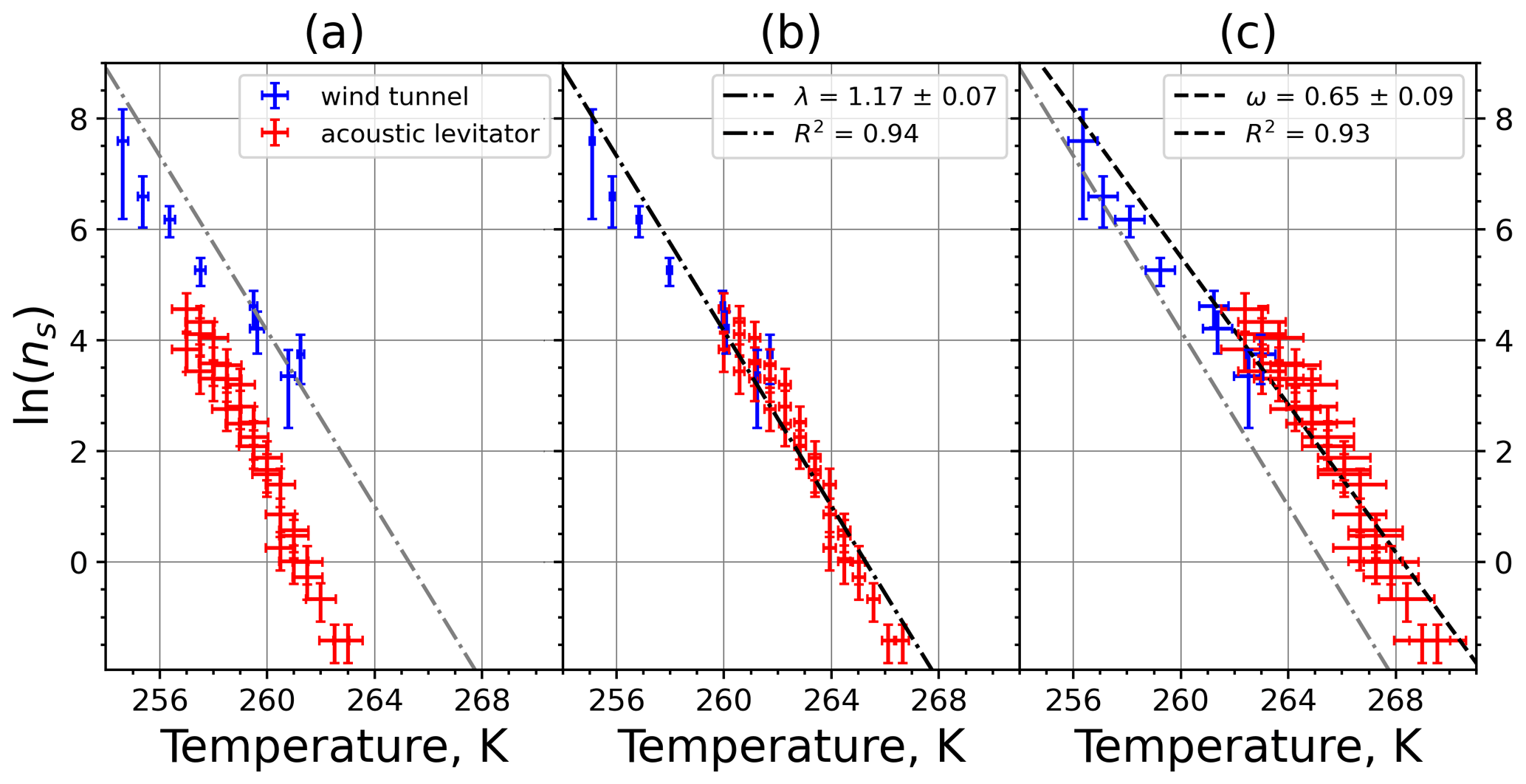
Figure A6 (a) Composite INAS density spectrum of feldspar from the uncorrected M-WT (blue) and M-AL (red) measurements. Panels (b) and (c) show the temperature-corrected data points from the M-WT and M-AL experiments based on λ and ω, respectively. The dash-dotted line in (c) is the regression line on corrected data points obtained by employing the optimal λ value as in (b).

A4 Illite NX

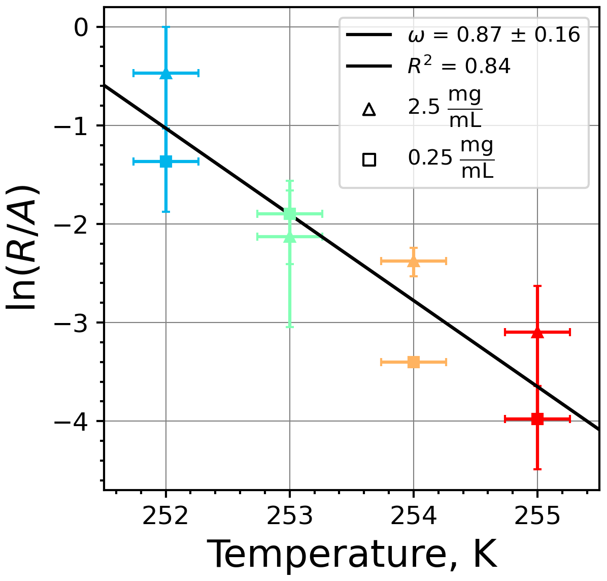
Figure A7 Freezing rate of illite NX normalized to surface area as a function of temperature for experiments at the M-WT with particle concentrations of 2.5 and 0.25 g L⁻¹ (plotted by triangles and rectangles, respectively). Freezing rates were calculated from the time dependence of the liquid ratio of illite NX presented in Fig. 6 in Diehl et al. (2014).

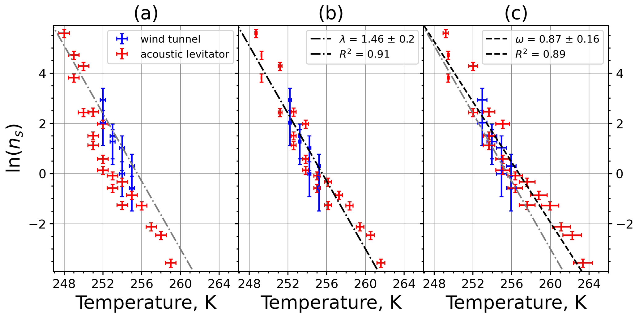
Figure A8 (a) Composite INAS density spectrum of illite NX from the uncorrected M-WT (blue) and M-AL (red) measurements. Panels (b) and (c) show the temperature-corrected data points from the M-WT and M-AL experiments based on λ and ω, respectively. The dash-dotted line in (c) is the regression line on corrected data points obtained by employing the optimal λ value as in (b).

A5 Montmorillonite

Figure A9 (a) The decrease in fraction of droplets which remained liquid with time at different temperatures in the isothermal experiments for montmorillonite at the M-WT. The colors correspond to different temperatures (particle concentrations of 5 g L⁻¹). Typical error bars are depicted in Fig. 6. (b) Freezing rate of montmorillonite normalized to surface area as a function of temperature.

Figure A10 (a) Composite INAS density spectrum of montmorillonite from the uncorrected M-WT (blue) and M-AL (red) measurements. Panels (b) and (c) show the temperature-corrected data points from the M-WT and M-AL experiments based on λ and ω, respectively. The dash-dotted line in (c) is the regression line on corrected data points obtained by employing the optimal λ value as in (b).

A6 Sahara dust SDB01

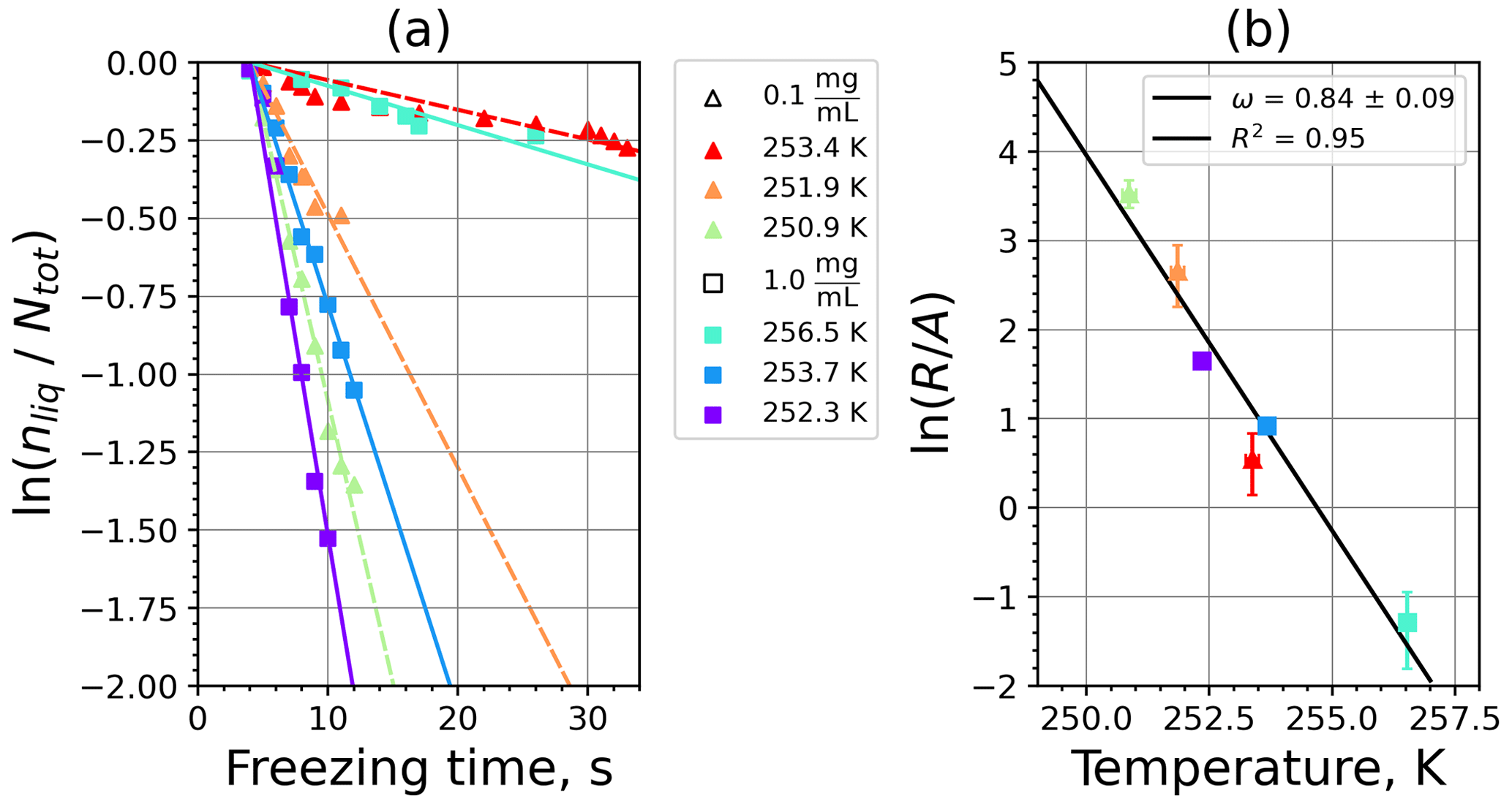
Figure A11 (a) The decrease in fraction of droplets which remained liquid with time at different temperatures in the isothermal experiments for Sahara dust at the M-WT. The colors correspond to different temperatures (particle concentrations of 5 g L⁻¹). Typical error bars are depicted in Fig. 6. (b) Freezing rate of Sahara dust normalized to surface area as a function of temperature.

Figure A12 (a) Composite INAS density spectrum of Sahara dust from the uncorrected M-WT (blue) and M-AL (red) measurements. Panels (b) and (c) show the temperature-corrected data points from the M-WT and M-AL experiments based on λ and ω, respectively. The dash-dotted line in (c) is the regression line on corrected data points obtained by employing the optimal λ value as in (b).

Appendix B: Drop temperature adaptation in the M-AL and in the M-WT

A liquid droplet placed in a colder or warmer environment tends to a quasi-steady-state temperature difference between itself and its surroundings. In order to describe the temperature adaptation process, diffusional and convective transfer of heat and mass for water vapor is considered. We follow the concept of Pruppacher and Klett (2010) in the forthcoming derivation. Hence, first, the heat and mass transfer of a motionless droplet is described, and after that the effect of air ventilation is introduced. The symbols used here are listed in Appendix C.

B1 Diffusional heat and mass transfer of a motionless drop in equilibrium

When computing the simple case of the diffusional heat transfer of a motionless water droplet in air, latent heat from condensation or evaporation is not considered. The rate of heat is calculated by integrating the heat flux density over the entire droplet surface. The heat flux density can be derived from Fourier's law, which in spherical coordinates reads as

$$\begin{array}{}\text{(B1)}& j_{\mathrm{h},r}{|}_{r=a}=-k_a{\left({\displaystyle \frac{\partial T}{\partial r}}\right)}_{r=a},\end{array}$$

where r is the distance from the drop center. Thus, the rate of heat transfer of a motionless drop considering pure diffusional heat transfer is

$$\begin{array}{}\text{(B2)}& {\left({\displaystyle \frac{\mathrm{d}q}{\mathrm{d}t}}\right)}_{\mathrm{0}}=-k_a\underset{S}{\int }{\left({\displaystyle \frac{\partial T}{\partial r}}\right)}_{r=a}dS.\end{array}$$

The temperature is determined by solving the heat conduction equation, which has its form in spherical coordinates for a motionless drop under steady-state thermal conditions:

$$\begin{array}{}\text{(B3)}& {\displaystyle \frac{{\partial }^{\mathrm{2}}T}{\partial r^{\mathrm{2}}}}+{\displaystyle \frac{\mathrm{2}}{r}}{\displaystyle \frac{\partial T}{\partial r}}=\mathrm{0}.\end{array}$$

This partial differential equation is solved using the boundary conditions

$$\begin{array}{}\text{(B4)}& {\displaystyle }T(r=\mathrm{\infty })=T_{\mathrm{\infty }}\text{(B5)}& {\displaystyle }T(r=a)=T_{\mathrm{a}}.\end{array}$$

where T_∞ is the temperature in the free air, i.e., far away from the drop, and T_a is the drop surface temperature, while a is the drop radius. The solution for the temperature as a function of r is

$$\begin{array}{}\text{(B6)}& T\left(r\right)=T_{\mathrm{\infty }}+\left(T_{\mathrm{a}}-T_{\mathrm{\infty }}\right){\displaystyle \frac{a}{r}}.\end{array}$$

Hence,

$$\begin{array}{}\text{(B7)}& {\left({\displaystyle \frac{\mathrm{d}q}{\mathrm{d}t}}\right)}_{\mathrm{0}}=\mathrm{4}\mathit{\pi }a{k}_a\left(T_{\mathrm{\infty }}-T_{\mathrm{a}}\right).\end{array}$$

Similarly to the heat transfer, the mass transfer rate of a motionless droplet in equilibrium with its surrounding air is calculated from

$$\begin{array}{}\text{(B8)}& {\left({\displaystyle \frac{\mathrm{d}m}{\mathrm{d}t}}\right)}_{\mathrm{0}}=-D_{\mathrm{v}}\underset{S}{\int }{\left({\displaystyle \frac{\partial {\mathit{\rho }}_{\mathrm{v}}}{\partial r}}\right)}_{r=a}\mathrm{d}S,\end{array}$$

where D_v is the water vapor diffusion coefficient, and ρ_v is the water vapor density in the surrounding air around the water droplet. The water vapor density can be found by solving the convective-diffusion equation:

$$\begin{array}{}\text{(B9)}& {\displaystyle \frac{\partial {\mathit{\rho }}_{\mathrm{v}}}{\partial t}}+\mathrm{\nabla }{\mathit{\rho }}_{\mathrm{v}}u=D_{\mathrm{v}}{\mathrm{\nabla }}^{\mathrm{2}}{\mathit{\rho }}_{\mathrm{v}}.\end{array}$$

This differential equation is simplified for a motionless drop in a steady state to Laplace's equation in the form ∇²ρ_v=0 (cf. Eq. B3). The boundary conditions for the problem are

$$\begin{array}{}\text{(B10)}& {\displaystyle }{\mathit{\rho }}_{\mathrm{v}}(r=\mathrm{\infty })={\mathit{\rho }}_{\mathrm{v},\mathrm{\infty }}\text{(B11)}& {\displaystyle }{\mathit{\rho }}_{\mathrm{v}}(r=a)={\mathit{\rho }}_{\mathrm{v},a},\end{array}$$

where ρ_v,∞ and ρ_v,a are the water vapor densities in the air far away from the drop and at the drop surface, respectively. The solution of the governing differential equation is similar to that for the heat transfer. Thus, the rate of change in the mass of a motionless droplet due to diffusion of water vapor under steady-state conditions is given by

$$\begin{array}{}\text{(B12)}& {\left({\displaystyle \frac{\mathrm{d}m}{\mathrm{d}t}}\right)}_{\mathrm{0}}=\mathrm{4}\mathit{\pi }{D}_{\mathrm{v}}\left({\mathit{\rho }}_{\mathrm{v},\mathrm{\infty }}-{\mathit{\rho }}_{\mathrm{v},a}\right).\end{array}$$

B2 Heat and mass transfer of an evaporating drop in airflow

We now consider the more realistic and atmospherically relevant case involving also the effect of air motion around the droplet. The total rate at which a drop falling in air gains heat is the sum of the convective heat flux from the air to the drop and the heat loss of the drop by releasing latent heat due to evaporation:

$$\begin{array}{}\text{(B13)}& {\left({\displaystyle \frac{\mathrm{d}q}{\mathrm{d}t}}\right)}_a=\mathrm{4}\mathit{\pi }a{k}_a\left(T_{\mathrm{\infty }}-T\left(t\right)\right)\cdot f_{\mathrm{h}}+L_e{\displaystyle \frac{\mathrm{d}m}{\mathrm{d}t}}\cdot f_{\mathrm{v}},\end{array}$$

where the so-called ventilation coefficients f_h and f_v are introduced, accounting for the enhanced heat and mass transfer, respectively, due to ventilation. Thus, for a drop in an airflow f_h>1 and f_v>1, while a motionless evaporating drop can be described using Eq. (B13) by setting f_h=1 and f_v=1. In the M-AL or in M-WT, where a warm (≈20 ^∘C) drop is injected into a cold subsaturated environment, both terms on the right-hand side of Eq. (B13) are negative. The drop cools down at a rate proportional to its mass m determined by

$$\begin{array}{}\text{(B14)}& {\left({\displaystyle \frac{\mathrm{d}q}{\mathrm{d}t}}\right)}_a=m{c}_{\mathrm{w}}{\displaystyle \frac{\mathrm{d}}{\mathrm{d}t}}\left(T_{\mathrm{a}}-T_{\mathrm{\infty }}\right),\end{array}$$

where c_w is the specific heat capacity of water. By equating Eqs. (B13) and (B14) we get the governing equation for the temperature adaptation of the droplet as

$$\begin{array}{}\text{(B15)}& \begin{array}{rl}{\displaystyle \frac{\mathrm{4}\mathit{\pi }}{\mathrm{3}}}& a^{\mathrm{3}}{\mathit{\rho }}_{\mathrm{w}}{c}_{\mathrm{w}}{\displaystyle \frac{\mathrm{d}}{\mathrm{d}t}}\left(T_{\mathrm{\infty }}-T_{\mathrm{a}}\left(t\right)\right)\\ & =-\mathrm{4}\mathit{\pi }a{k}_a\left(T_{\mathrm{\infty }}-T_{\mathrm{a}}\left(t\right)\right)\cdot f_{\mathrm{h}}\\ & -\mathrm{4}\mathit{\pi }a{L}_e{D}_{\mathrm{v}}\left({\mathit{\rho }}_{\mathrm{v},\mathrm{\infty }}-{\mathit{\rho }}_{\mathrm{v},a}\right)\cdot f_{\mathrm{v}}.\end{array}\end{array}$$

After integration, we obtain the following solution of this differential equation:

$$\begin{array}{}\text{(B16)}& T_{\mathrm{\infty }}-T_{\mathrm{a}}\left(t\right)-\mathit{\delta }=\left(T_{\mathrm{\infty }}-T_{\mathrm{a}}(t=\mathrm{0})-\mathit{\delta }\right)\exp \left(-t/\mathit{\tau }\right),\end{array}$$

with the time constant

$$\begin{array}{}\text{(B17)}& \mathit{\tau }={\displaystyle \frac{a^{\mathrm{2}}{\mathit{\rho }}_{\mathrm{w}}{c}_{\mathrm{w}}}{\mathrm{3}\left[k_a{L}_e{D}_{\mathrm{v}}{\left(\frac{\mathrm{d}{\mathit{\rho }}_{\mathrm{v}}}{\mathrm{d}T}\right)}_{\mathrm{sat}}\right]\cdot f_{\mathrm{h}}}}\end{array}$$

and

$$\begin{array}{}\text{(B18)}& \mathit{\delta }={\displaystyle \frac{D_{\mathrm{v}}{L}_e{f}_{\mathrm{v}}\left[\frac{\mathrm{1}-r_{\mathrm{v}}}{r_{\mathrm{v}}}{\mathit{\rho }}_{\mathrm{v},\mathrm{\infty }}\right]}{k_a\cdot f_{\mathrm{h}}+L_e{D}_{\mathrm{v}}{f}_{\mathrm{v}}{\left(\frac{\mathrm{d}{\mathit{\rho }}_{\mathrm{v}}}{\mathrm{d}T}\right)}_{\mathrm{sat}}}},\end{array}$$

which gives the steady temperature difference between the equilibrium temperature ($T_{\mathrm{e}}=T_{\mathrm{a}}(t\to \mathrm{\infty })$) of a ventilated evaporating drop and its surrounding air at a relative humidity of r_v. For simplicity we did not indicate that the physical quantities are represented by their averages over the integration interval. Furthermore, we assumed that f_h=f_v (Pruppacher and Klett, 2014).

After some manipulation and using ${\mathit{\rho }}_{\mathrm{v},\mathrm{sat}}\left(T_{\mathrm{e}}\right)={\mathit{\rho }}_{\mathrm{v},a}\left(T_{\mathrm{e}}\right)$, one can get two other forms for δ:

$$\begin{array}{}\text{(B19)}& \mathit{\delta }={\displaystyle \frac{D_{\mathrm{v}}{L}_e{f}_{\mathrm{v}}\left[{\mathit{\rho }}_{\mathrm{v},\mathrm{sat}}\left(T_{\mathrm{e}}\right)-{\mathit{\rho }}_{\mathrm{v},\mathrm{\infty }}\right]}{k_a\cdot f_{\mathrm{h}}}}\end{array}$$

or by applying the ideal gas law

$$\begin{array}{}\text{(B20)}& \mathit{\delta }={\displaystyle \frac{D_{\mathrm{v}}{L}_e{f}_{\mathrm{v}}}{k_a\cdot f_{\mathrm{h}}}}{\displaystyle \frac{M_{\mathrm{w}}}{R}}\left({\displaystyle \frac{e_{\mathrm{sat}}\left(T_{\mathrm{e}}\right)}{T_{\mathrm{e}}}}-{\displaystyle \frac{e_{\mathrm{\infty }}}{T_{\mathrm{\infty }}}}\right),\end{array}$$

where e_sat(T_e) is the saturation water vapor pressure at temperature T_e, and e_∞ is the water vapor pressure in the air. Hence, the equilibrium drop temperature is given as

$$\begin{array}{}\text{(B21)}& T_{\mathrm{e}}=T_{\mathrm{\infty }}-{\displaystyle \frac{D_{\mathrm{v}}{L}_e{f}_{\mathrm{v}}}{k_a\cdot f_{\mathrm{h}}}}{\displaystyle \frac{M_w}{R}}\left({\displaystyle \frac{e_a\left(T_{\mathrm{e}}\right)}{T_{\mathrm{e}}}}-{\displaystyle \frac{e_{\mathrm{\infty }}}{T_{\mathrm{\infty }}}}\right).\end{array}$$

In the M-AL the levitating drop may gain heat from the absorbed acoustic energy at a certain constant rate:

$$\begin{array}{}\text{(B22)}& {\displaystyle \frac{\mathrm{d}{q}_{\mathrm{ac}}}{\mathrm{d}t}}=e_{\mathrm{ac}}V,\end{array}$$

where e_ac is the acoustic energy density flux, and V is the drop volume; e_ac varies with time at a very high frequency (≈20 kHz), and therefore it can be considered to be time-independent when discussing the slow process of heat transfer. Since this term is independent of temperature and time, it does not affect τ and does not appear in Eq. (B17), which describes the time dependence of the temperature adaptation process. Nevertheless, the absorbed acoustic energy heats up the drop and increases δ with a constant temperature value. This temperature difference between the theoretically calculated equilibrium temperature and the environmental temperature was also observed in the M-AL and calculated to be ≈4.5 K.

B3 Drop surface temperature in the M-AL

Although there is seemingly no airflow around a drop levitating in the M-AL, the pressure distribution caused by the acoustic waves does create convection about it (Lierke, 1995). This has to be considered in the temporal-evolution calculation in Eq. (B17). In Fig. B1 an example of the measured surface temperature evolution of a 2 mm diameter drop placed into the M-AL is plotted by a black line. Neglecting ventilation around the drop (i.e., f_v=1.0 in Eq. B17), the cooling would be much slower (blue line) than in reality. Setting the ventilation coefficient to f_v=5.2 – the value of which is close to f_v=3 determined by Lierke (1995) – the temperature evolution accurately follows the measured curve (green line).

Figure B1 Temporal evolution of the surface temperature of a 2 mm diameter drop injected into the M-AL: measured (black line), calculated using Eq. (B16) without ventilation (blue line), calculated using Eq. (B16) with a ventilation factor f_v=5.2 (green line).

B4 Simulation of the internal drop temperature in the M-AL

In M-AL experiments the continuous sharp surface temperature drop caused by the adaptation to the significantly colder environment results in a temperature difference in the drop interior. Therefore, the temperature at the drop surface is lower than close to the drop center. Since the drop temperature was determined in the M-AL experiments by measuring the surface temperature by means of an infrared thermometer, the actual (internal) temperature experienced by ice-nucleating particles inside the drop is higher than the measured value. This measurement artifact might falsify the experimentally determined temperature dependence of the ice-nucleating ability. In order to estimate this experimental issue, a simulation was carried out based on the theoretical formulation of the temperature adaptation given above and on heat conduction inside the liquid drop. The drop volume was split into 10 layers of equivalent radii, and the heat conduction among the layers was calculated by solving the transient-heat equation:

$$\begin{array}{}\text{(B23)}& {\displaystyle \frac{\partial T}{\partial t}}={\displaystyle \frac{{\partial }^{\mathrm{2}}T}{\partial r^{\mathrm{2}}}}+{\displaystyle \frac{\mathrm{2}}{r}}{\displaystyle \frac{\partial T}{\partial r}}.\end{array}$$

For the numerical integration, the explicit finite-difference method was used. During the simulation the surface temperature was continuously cooling following the experimentally obtained adaptation curve shown in Fig. B1. The temperature distribution inside the drop is depicted at four time instances (i.e., drop surface temperatures) in Fig. B2, revealing the temperature difference between the drop surface and the drop center.

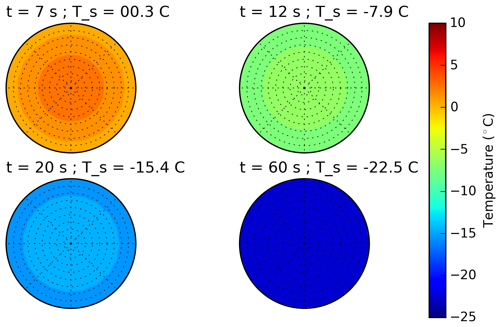
Figure B2 Internal temperatures at four different time instances for a continuously cooling drop of 2 mm diameter in the M-AL following Fig. B1 based on numerical simulation of the heat conduction equation.

The temperature variation in three layers together with the volume-averaged drop temperature change relative to the surface temperature is further investigated in Fig. B3. While the temperature at the drop's center (red curve) deviates from the surface temperature by up to 2.5 ^∘C, the second-outermost layer, representing 40 % of the entire drop volume (green curve), follows the surface temperature within 0.5 ^∘C at subzero temperatures. At temperatures below −5 ^∘C, which are relevant for immersion freezing experiments, the temperature difference is less than 0.3 ^∘C, thus within the measurement uncertainties. The volume-averaged drop temperature (magenta curve in Fig. B3) is also within the measurement uncertainty of 0.5 ^∘C for this temperature range.

The simulation was carried out without considering any internal circulation, which would further and faster unify the temperature distribution inside the liquid. Considering the large number of ice-nucleating particles (≳ 300 000) immersed in each of the drops, one can conclude that the surface temperature measured by the pyrometer can be used as a characteristic drop temperature.

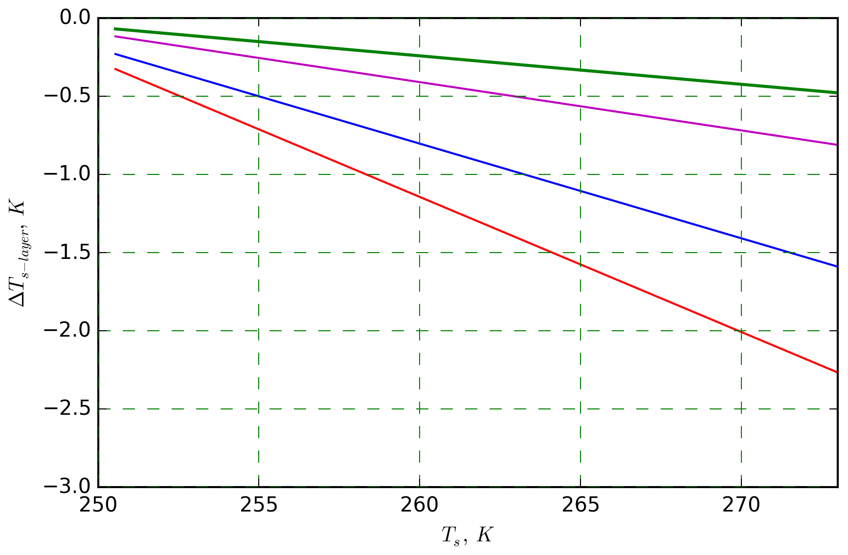
Figure B3 Temperature difference between the drop surface and internal drop layers calculated from the numerical simulation: drop center (red curve); layers number 5 (blue) and 8 (green), representing 20 % and 60 % of entire drop volume, respectively; and volume-averaged temperature (magenta).

The temperature difference between the surface and the volume-averaged temperature of the drop is compared to the temperature shift calculated for three different λ values in Fig. B4. The figure reveals that the calculated temperature difference inside the drop (magenta curve) is a factor of 6 to 20 smaller than the temperature shift caused by the high cooling rate in the M-AL for different λ values (red, green, and blue lines). Therefore, this effect cannot explain the observed freezing-temperature shift in the M-AL.

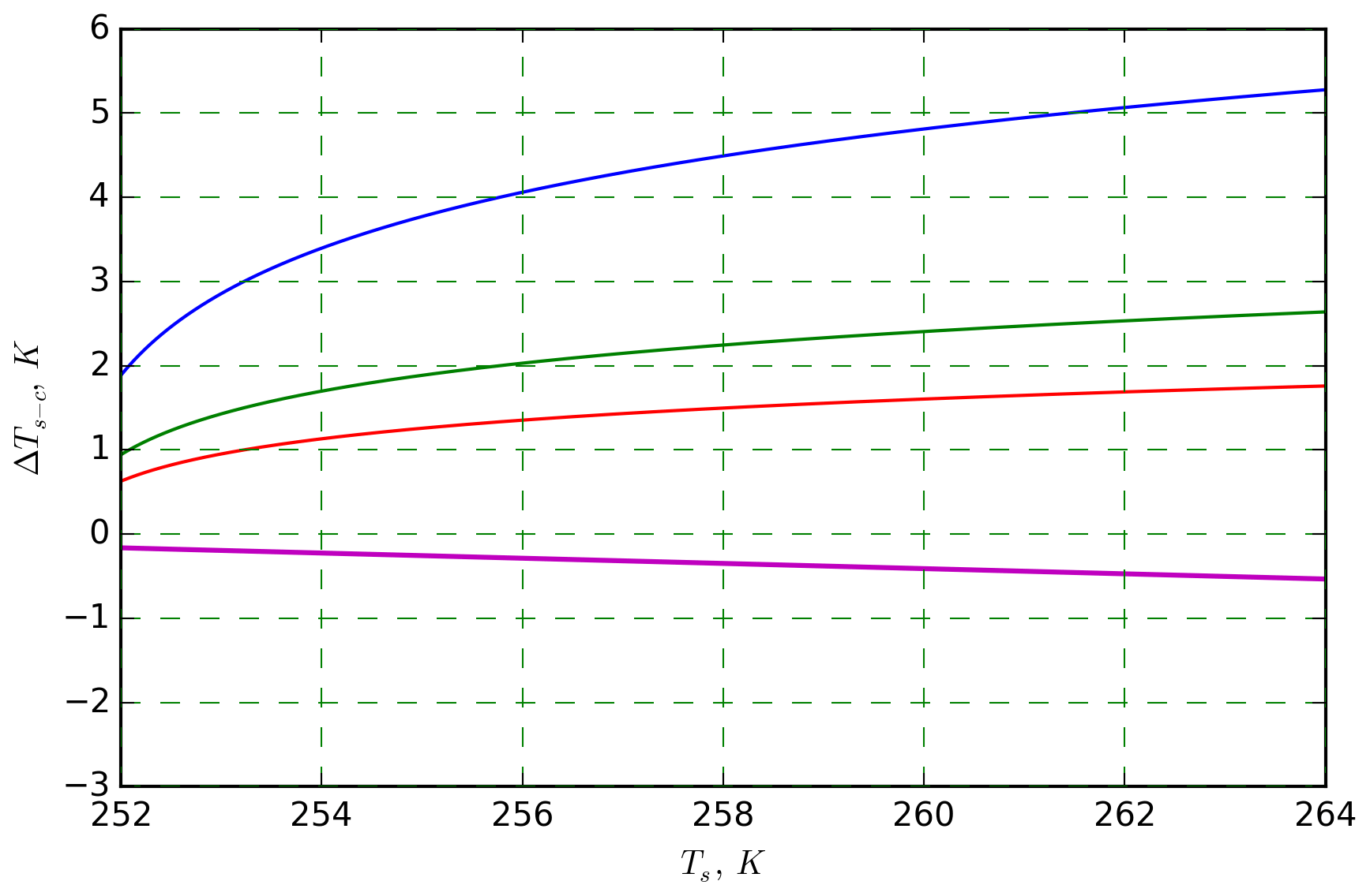
Figure B4 Temperature shift calculated for three different λ values (red: 0.8; green: 1.6; and blue: 2.4) in relation to temperature difference between drop surface and volume-averaged drop temperature (magenta curve).

B5 Procedure chart for data evaluation

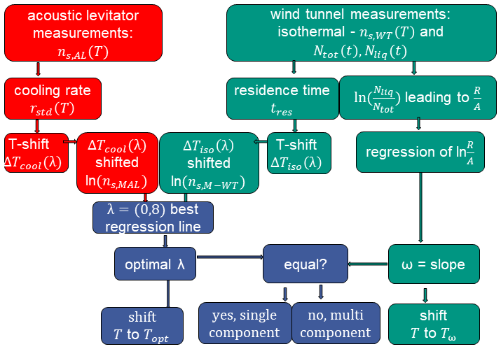
Figure B5 Flowchart of the procedure used to combine M-WT and M-AL measurement data for determining λ and ω and classifying the investigated materials as single- or multiple-component. Red and green boxes correspond to M-Al and M-WT data, respectively.

Appendix C: List of symbols

β	Freezing-temperature shift for water vapor (Vali, 2014)
δNfr	Number of droplets freezing within time interval δt
ΔTiso	Temperature shift in isothermal experiments due to a relative change in residence time
ΔTr, ΔTf	Absolute and normalized temperature shifts, respectively, in cooling experiments due to any change in cooling rate
δ	Temperature difference between a drop and its environment in equilibrium (i.e., $\mathit{\delta }=T_{\mathrm{\infty }}-T_{\mathrm{e}})$)
λ	Temperature gradient (K−1) of the heterogeneous-nucleation-rate coefficient, Js
ω	Temperature gradient (K−1) of the freezing rate
τ	Time constant of the temperature adaptation of a drop placed in colder or warmer environment
A	Total particle surface area
c	Particle mass concentration in the sample solution
fice	Cumulative fraction of droplets frozen between 0 ∘C and temperature T
Js	Heterogeneous-nucleation-rate coefficient of a single-component system
Jhom	Homogeneous-nucleation-rate coefficient
ns	Ice-nucleation-active-site density
nfr, nliq	Number of frozen and liquid droplets in a freezing experiment, respectively
Ntot	Total number of droplets in the population
R(T)	Freezing rate at a fixed temperature
R(t,T)	Rate of supercooled droplets freezing per unit time at a fixed temperature
r	Cooling rate in the experiments
sω, sλ	Error-weighted standard deviations of the residuals for ω and λ
SSA	Specific surface area of the particle
T	Temperature
t	Measurement time
Ta	Drop surface temperature
Te	Equilibrium temperature between ventilated evaporating droplet and its environment
T∞	Air and environmental temperature
ts,ω, ts,λ	t numbers corresponding to ω and λ calculated for applying a two-sided Student t test
tsig	t number corresponding to a significance level of 99.9 % in a two-sided Student t test
Vd	Aqueous-suspension drop volume