Assessment of meteorology vs. control measures in the China fine particular matter trend from 2013 to 2019 by an environmental meteorology index

A framework was developed to quantitatively assess the contribution of meteorology variations to the trend of fine particular matter (PM_2.5) concentrations and to separate the impacts of meteorology from the control measures in the trend, based upon the Environmental Meteorology Index (EMI). The model-based EMI realistically reflects the role of meteorology in the trend of PM_2.5 and is explicitly attributed to three major factors: deposition, vertical accumulation and horizontal transports. Based on the 2013–2019 PM_2.5 observation data and re-analysis meteorological data in China, the contributions of meteorology and control measures in nine regions of China were assessed separately by the EMI-based framework. Monitoring network observations show that the PM_2.5 concentrations have declined by about 50 % on the national average and by about 35 % to 53 % for various regions. It is found that the nationwide emission control measures were the dominant factor in the declining trend of China PM_2.5 concentrations, contributing about 47 % of the PM_2.5 decrease from 2013 to 2019 on the national average and 32 % to 52 % for various regions. The meteorology has a variable and sometimes critical contribution to the year-by-year variations of PM_2.5 concentrations, 5 % on the annual average and 10 %–20 % for the fall–winter heavy pollution seasons.

1 Introduction

Recent observation data from the Ministry of Ecology and Environment of China (MEE) have shown a steady improvement of air quality across the country, especially in particular matter (PM) concentrations (Hou et al., 2019). According to the 2013–2019 China Air Quality Improvement Report issued by the MEE, compared to 2013, the average concentrations of particulate matter with an aerodynamic diameter of less than 2.5 µm (PM_2.5) in 74 major cities of China decreased by more than 50 % in 2019. From scientific and management point of views, a quantitative apportionment of the reasons behind the trend is critical to assess the reduction strategies implemented by the government and to guide future air quality control policy. However, the assessment of the improvements of air quality is a complicated process that involves the quantification of changes in the emission sources, meteorological factors, and other characteristics of the PM_2.5 pollution, which are also interacting with each other. In order to separate the relative degree of these factors, a comprehensive analysis, including observational data and model simulation, is needed.

Studies have been done extensively on the impacts of weather systems on air quality. Synoptic and local meteorological conditions have been recognized as influencing the PM concentrations at various scales (Beaver and Palazoglu, 2006; He et al., 2017a, b; Pearce et al., 2011a, b). For the atmospheric aerosol pollution, the dynamic effect of the downdraft in the “leeward slope” and “weak wind area” of the Qinghai Tibet Plateau in winter is not conducive to the diffusion of air pollution emissions in the urban agglomerations of eastern China (Xu et al., 2015, 2002). The evolution of circulation situation is an important factor driving the change in haze pollution (He et al., 2018). The local circulations, such as mountain and valley wind and urban island circulation, have a significant impact on local pollutant concentration (Chen et al., 2009; Yu et al., 2016). Previous studies also revealed that PM_2.5 concentration is significantly correlated with local meteorological elements, such as temperature, humidity, wind speed, and boundary layer height (He et al., 2017b; Bei et al., 2020; Ma et al., 2019; He et al., 2016).

In the Beijing–Tianjin–Hebei (BTH) region, a correlation analysis and principal component regression method (Zhou et al., 2014) was used to identify the major meteorological factors that influenced the API (Air Pollution Index) time series in China from 2001 to 2010, indicating that air pressure, air temperature, precipitation and relative humidity were closely related to air quality with a series of regression formulas. Yet the analysis was assumed to be a relatively unchanged emission whose impacts were not taken into account. On a local scale, an attempt (Zhang et al., 2017) was made to correlate the air pollutant levels with a combination of meteorological factors with the development of the Stable Weather Index (SWI) at the China Meteorological Administration (CMA). The SWI is a composite index which includes the advection, vertical diffusion and humidity and other meteorological factors that are related to the formation of air pollutions in a specific region or city. A higher value of SWI means a weaker diffusion of air pollutants. This index had some success in assessing the meteorological impacts on air pollution, especially calibrated for a specific region, i.e., Beijing. However, when applied to different areas where the emission patterns and meteorological features are different, this index failed to give a universal or comparable indication of meteorological assessment of pollution levels across the nation.

Using the Kolmogorov–Zurbenko (KZ) wave filter method, Bai et al. (2015) separated the API time series into three Chinese cities into short-term, seasonal and long-term components and then used the stepwise regression to set up API baseline and short-term components separately and established linear regression models for meteorological variables of corresponding scales. Consequently, with the long term representing the change in emissions removed from the time series, the meteorological contributions alone were assumed and analyzed, pointing out that unfavorable conditions often lead to an increase by 1–13 and the favorable conditions to a decrease by 2–6 in the long-term API series, respectively. Though the contributions of emissions and meteorological variations were separated by the research, it was only done by mathematical transformations and far from the reality. The mechanisms behind the variation of the time series were not investigated.

A chemical transport model (CTM) is an ideal tool to carry the task of assessment by taking the meteorology, emissions and processes into consideration altogether. Andersson et al. (2007) used a CTM to study the meteorologically induced inter-annual variability and trends in deposition of sulfur and nitrogen as well as concentrations of surface ozone (O₃), nitrogen dioxide (NO₂) and PM and its constituents over Europe during 1958–2001. It is found that the average European interannual variation, due to meteorological variability, ranges from 3 % for O₃, 5 % for NO₂, 9 % for PM, 6 %–9 % for dry deposition, to about 20 % for wet deposition of sulfur and nitrogen. A multi-model assessment of air quality trends with constant anthropogenic emissions was also carried out in Europe (Colette et al., 2011) and found that the magnitude of the emission-driven trend exceeds the natural variability for primary compounds, concluding that emission management strategies have had a significant impact over the past 10 years, hence supporting further emission reduction strategies. Model assessments of air quality trends in various regions and time periods (Wei et al., 2017; Li et al., 2015) in China were also done and yielded some useful results. For the BTH region, Li et al. (2015) used the Comprehensive Air Quality Model with extensions (CAMx) plus the Particulate Source Apportionment Technology (PSAT) to simulate the contributions of emission changes in various sectors and changes in meteorology conditions for the PM_2.5 trend from 2006 to 2013. It was found that the change in source contribution of PM_2.5 in Beijing and northern Hebei was dominated by the change in local emissions. However, for Tianjin and central and southern Hebei Province, the change in meteorology conditions was as important as the change in emissions, illustrating the regional difference of impacts by meteorology and emissions. However, the emission changes in the simulations were assumed and did not reflect the real spatio-temporal variations.

There is no surprise that previous studies could not systematically catch the meteorological impacts across the whole nation as the controlling meteorological factors involving the characteristics of plenary boundary layers (PBLs), wind speed and turbulence, temperature and stability, radiation and clouds, underlying surface as well as pollutant emissions vary greatly from region to region. A single index or correlation cannot be applied to the entire nation. Obviously, in order to systematically assess the impacts of meteorology on air pollution, these factors have to be taken into consideration in a framework and be assessed simultaneously. This paper presents a methodology to assess the individual impacts of meteorology and emission changes, based on a model-derived index EMI, i.e., Environmental Meteorology Index, and observational data, providing a comprehensive analysis of the air quality trends in various regions of China, with mechanistic and quantitative attributions of various factors.

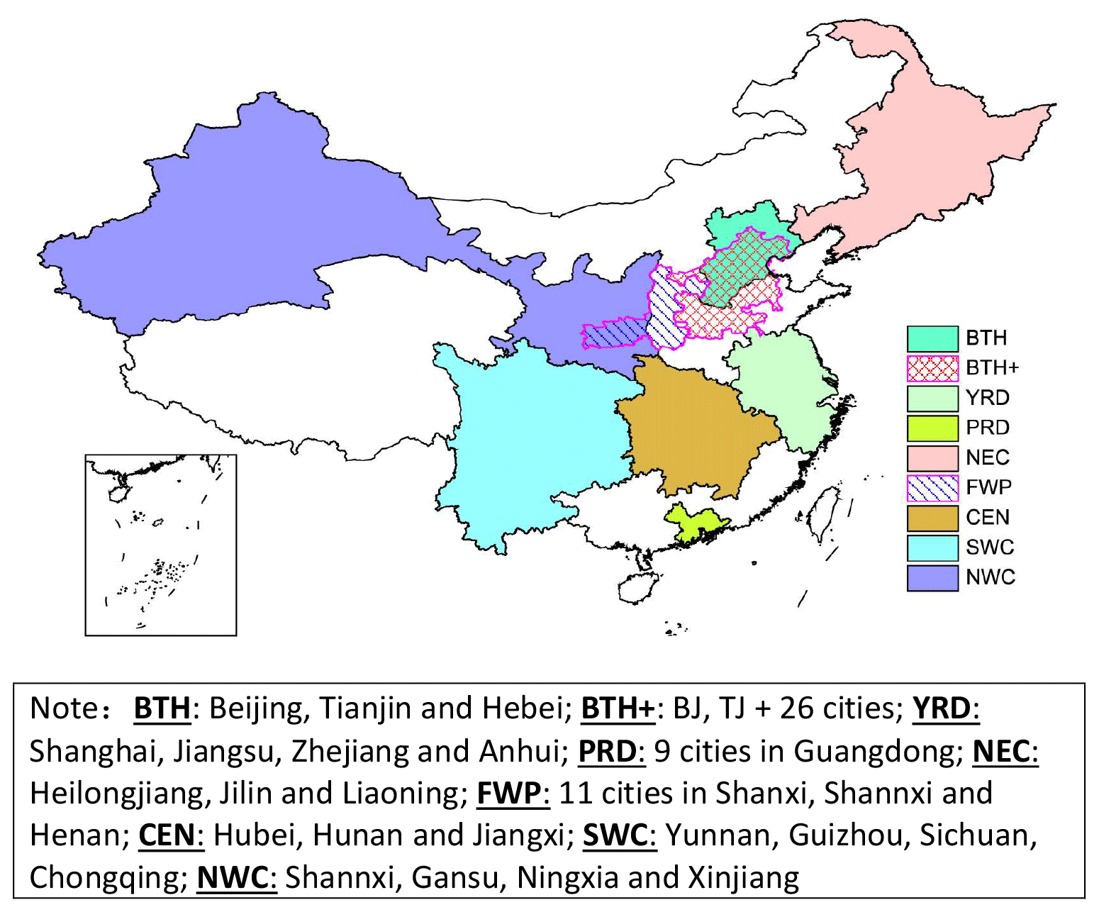
Figure 1 Analysis region separation and definition.

2 Methodology

The assessment is carried out through the combination of observational data and the EMI from model analysis. Since the emission and air quality characteristics vary greatly from region to region in China, the analysis is divided into nine focused regions (Fig. 1). Regional air quality data (PM_2.5) provides the basis for the trend analysis. Separating the trend contribution from regional emission reduction and meteorological variation entails a framework which is discussed below.

Figure 2 National and regional trend lines of PM_2.5 in China from 2013 to 2019.

2.1 Particular matter (PM) observation data

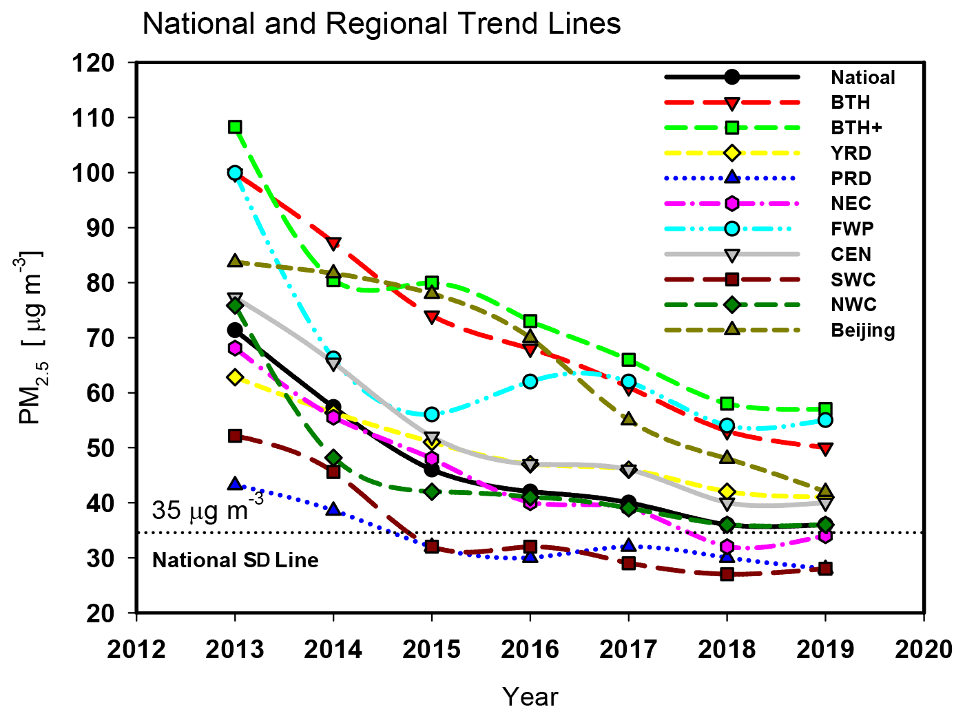
The observational pollution data of PM_2.5 concentrations used in this study were from the monitoring network of the MEE of China (http://english.mee.gov.cn/, last access: 31 December 2020). From 2013 to 2019, the concentrations showed a large change in the country, where most regions saw a declined trend in the annual concentrations. Data show that from 2013 to 2019, the national annual averaged PM_2.5 concentrations dropped about 50 % (Fig. 2), where the haze days have been shortened by 21.2 d from the CMA monitoring data (Table 1), with some regional differences. Regionally, by 2019, the PM_2.5 reduction rate from 2013 ranged from 35 % to 53 %. Detailed analysis will be carried out in the Results and discussions section.

Table 1 National and regional environmental meteorology in 2019 and comparisons with 2015 and 2013.

Note: “+” increased; “−” decreased.

It is noted that the PM_2.5 mass concentrations by the MEE are now reported under the observation site's actual conditions of temperature and pressure from 1 September 2018, before which the values were reported under the standard state (STP), i.e., 273 K and 101.325 kPa. In order to maintain the consistency of the data series, the PM_2.5 concentrations used in this study have all been converted according to the new standard (MEE, 2012) (GB3095-2012) under actual conditions. Research has shown that after the change in reporting standard, the PM_2.5 concentration in most cities decreased, and the number of good days to meet the standard increased (Zhang and Rao, 2019).

2.2 Meteorological data

Conventional meteorological data can provide qualitative assessment of the contributions of meteorological factors to the changes in air quality. The data used in this study are from 843 national base weather stations of the CMA from 2013 to 2019. The wind speed (WS), day with small wind (DSW), relative humidity (RH) and haze days are used to analyze the pollution meteorological conditions. When the daily average wind speed is less than 2 m s⁻¹, a DSW is defined. Since the haze formation is always related to stable meteorological conditions and high aerosol mass loading, haze observation from the CMA is also used to analyze the haze trends and the impact of air quality on visibility. A haze day is defined with daily averaged visibility less than 10 km and relative humidity less than 85 % (Wu et al., 2014), excluding days of low visibility due to precipitation, blowing snow, blowing sand, floating dust, sandstorms and smoke.

The 2019 national annual averaged WS increased by 4.5 %, DSW dropped by 15.1 %, and RH decreased by 3.9 % compared with 2013, with regional differences (Table 1). Slight changes occurred when compared with 2015: WS decreased by 0.7 %, DSW dropped by 11.3 %, and RH decreased by 2.2 %. Overall, it can be seen that the annual haze days have a certain degree of correlations negatively with WS and positively with DSW. Detailed analysis linking PM_2.5 and meteorology will be given in the Results and discussions section.

2.3 EMI – the Environmental Meteorological Index

Due to the complicated interactions of emissions, meteorology and atmospheric processes, a single set of meteorological factors or a combination of them cannot quantitatively attribute the individual factor to the changes in concentration observed.

In order to quantitatively assess the impacts of meteorological conditions on the changes in air pollution levels, an EMI is defined as follows. For a defined atmospheric column (h) at a time t, an EMI is defined as an indication of atmospheric pollution level:

$$\begin{array}{}\text{(1)}& \mathrm{EMI}\left(t\right)=\mathrm{EMI}\left(t\mathrm{0}\right)+\underset{t\mathrm{0}}{\overset{t}{\int }}\mathrm{\Delta }\mathrm{EMI}\cdot \mathrm{d}t,\end{array}$$

where the ΔEMI is the tendency that causes the changes in pollution level in a time interval dt defined as

$$\begin{array}{}\text{(2)}& \mathrm{\Delta }\mathrm{EMI}=\text{iEmid}+\text{iTran}+\text{iAccu},\end{array}$$

where the iEmid is the difference between emission and deposition, and iTran and iAccu are the net (in minus out) advection transports and the vertical accumulation by turbulent diffusion in the column, respectively. A positive sign of each factor indicates a net flow of pollutants into the column, and vice versa.

Mathematically, these factors are expressed as

$$\begin{array}{}\text{(3)}& \begin{array}{rl}\text{iTran}& ={\displaystyle \frac{\mathrm{1}}{h{C}_{\mathrm{0}}}}\underset{\mathrm{0}}{\overset{h}{\int }}\left(u{\displaystyle \frac{\partial C}{\partial x}}+v{\displaystyle \frac{\partial C}{\partial y}}+w{\displaystyle \frac{\partial C}{\partial z}}\right)\mathrm{d}z,\\ \text{iAccu}& ={\displaystyle \frac{\mathrm{1}}{h{C}_{\mathrm{0}}}}\underset{\mathrm{0}}{\overset{h}{\int }}\left[{\displaystyle \frac{\partial C}{\partial x}}\left(K_x{\displaystyle \frac{\partial C}{\partial x}}\right)+{\displaystyle \frac{\partial C}{\partial y}}\left(K_y{\displaystyle \frac{\partial C}{\partial y}}\right)\right.\\ & \left.+{\displaystyle \frac{\partial C}{\partial z}}\left(K_z{\displaystyle \frac{\partial C}{\partial z}}\right)\right]\mathrm{d}z,\\ \text{iEmid}& ={\displaystyle \frac{\mathrm{1}}{h{C}_{\mathrm{0}}}}\underset{\mathrm{0}}{\overset{h}{\int }}\left[\text{Emis}-(V_{\mathrm{d}}+L_{\mathrm{d}})\right]\mathrm{d}z,\end{array}\end{array}$$

where the tendency is normalized by a factor C₀. For an application of the EMI to the PM_2.5, C₀ is set to equal 35 µg m⁻³, the national standard for PM_2.5 in China (MEE, 2012), and the EMI(t) is written as EMI(t)_2.5. If the EMI_2.5 is less than 1, the concentration level will reach or be better than the national standard.

It can be seen here that these key parameters account for the major meteorological factors which control the air pollutant levels, including wind speed and directions ($u,v,w$), turbulent diffusion coefficients ($K_x,K_y,K_z$) as well as dry and wet depositions (V_d and L_d). Therefore, under the conditions of unchanged emissions (Emis), the EMI variation reflects the impacts of meteorological factors on the levels of atmospheric pollutants. Furthermore, because of the inclusion of individual factors such as iTran, iAccu and iEmid, the variation of EMI(t)_2.5 can be attributed to the variation of each factor, which gives more detailed information on the meteorological influence on the ambient pollutant concentration variations. It should be pointed out that the current EMI has only accounted explicitly for three major physical processes of iTran, iAccu, and iEmid that are closely related to the meteorological influences. However, the secondary formation of aerosols is only implicitly considered in the EMI as the three major physical processes are calculated from the concentrations of aerosols (C) as indicated in Eq. (3).

Figure 3 Relationship between the ΔEMI, EMI(t)_2.5 and $\stackrel{\mathrm{‾}}{\text{EMI}(p{)}_{\mathrm{2.5}}}$.

For a period of time p (t0 to t1) when the averaged pollutant level (e.g., PM_2.5) is compared with EMI(t)_2.5, the time integral has to be done to obtain the averaged index for the period, such as

$$\begin{array}{}\text{(4)}& {\stackrel{\mathrm{‾}}{\text{EMI}\left(p\right)}}_{\mathrm{2.5}}={\displaystyle \frac{\mathrm{1}}{t\mathrm{1}-t\mathrm{0}}}\underset{t\mathrm{0}}{\overset{t\mathrm{1}}{\int }}\text{EMI}{\left(t\right)}_{\mathrm{2.5}}\mathrm{d}t.\end{array}$$

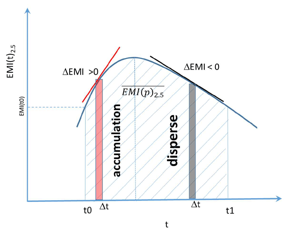
The relationship among the ΔEMI, EMI(t)_2.5 and ${\stackrel{\mathrm{‾}}{\text{EMI}\left(p\right)}}_{\mathrm{2.5}}$ is illustrated in Fig. 3. It is clear that the EMI(t)_2.5 is a function of time and can be used to reflect the pollution level at any time t, while the ${\stackrel{\mathrm{‾}}{\text{EMI}\left(p\right)}}_{\mathrm{2.5}}$ is the area under the EMI(t)_2.5 from times t0 to t1, which gives the averaged pollution levels for the period. The derivatives of EMI(t)_2.5 are the ΔEMI, which is a positive value when the pollution is being accumulated and a negative value when the pollution is being dispersed.

Therefore, for the period p with n discrete steps from t0 to t1, the ${\stackrel{\mathrm{‾}}{\text{EMI}\left(p\right)}}_{\mathrm{2.5}}$ represents the averaged meteorological influences on PM_2.5, while the sum of the positive ΔEMI is the accumulation potentials and the sum of the negative ΔEMI is the dispersing potentials as illustrated in Fig. 3. The relationship between them is derived as follows:

$$\begin{array}{}\text{(5)}& \begin{array}{rl}{\stackrel{\mathrm{‾}}{\text{EMI}\left(p\right)}}_{\mathrm{2.5}}& ={\displaystyle \frac{\mathrm{1}}{n+\mathrm{1}}}\left[\text{EMI}\left(\mathrm{0}\right)+\text{EMI}\left(\mathrm{1}\right)+\text{EMI}\left(\mathrm{2}\right)\right.\\ & \left.+\mathrm{\cdots }+\text{EMI}\left(n\right)\right]\\ & ={\displaystyle \frac{\mathrm{1}}{n+\mathrm{1}}}\left[(n+\mathrm{1})\text{EMI}\left(t\mathrm{0}\right)+n\mathrm{\Delta }\text{EMI}\left(\mathrm{1}\right)\mathrm{\Delta }t\right.\\ & +\left(n-\mathrm{1}\right)\mathrm{\Delta }\text{EMI}\left(\mathrm{2}\right)\mathrm{\Delta }t+\left(n-\mathrm{2}\right)\mathrm{\Delta }\text{EMI}\left(\mathrm{3}\right)\mathrm{\Delta }t\\ & \left.+\left(n-\mathrm{3}\right)\mathrm{\Delta }\text{EMI}\left(\mathrm{4}\right)\mathrm{\Delta }t+\mathrm{\dots }+\mathrm{\Delta }\text{EMI}\left(n\right)\mathrm{\Delta }t\right],\end{array}\end{array}$$

where n is the time steps in the period and the averaged EMI has been linked to the starting point EMI(0) and the changing rates of the EMI, i.e., ΔEMI(n), at each time step. For monthly simulations, the initial values EMI(t0) for each month were set up by the averaged PM_2.5 concentrations for the first day from 2013 to 2019 divided by the constant C₀ (35 µg m⁻³).

2.4 Assessment framework of emission controls

The EMI_2.5 index provides a way to assess the meteorological impacts on the changes in PM_2.5 concentrations at two time periods, i.e., January 2013 (p0) and January 2016 (p1), under the assumption of unchanged emissions. However, due to the national efforts of improving air quality, the year-by-year emissions are changing rapidly and unevenly across the country. The changes in both emissions and meteorology are tangled together to yield the observed changes in ambient concentrations. For policy makers, the emission reduction quantification is critical to guide further air quality improvements. The framework proposed here is to combine changes in the observed concentration levels and meteorology factors ${\stackrel{\mathrm{‾}}{\text{EMI}\left(p\right)}}_{\mathrm{2.5}}$ to quantify the changes caused by emission changes only at two time periods.

The observed concentrations at p0 and p1 are defined as PM (m0, e0) and PM (m1, e1), where (m0,e0) and (m1, e1) indicate the meteorology and emission status at p0 and p1, respectively. The contribution to the observed concentration changes between p0 and p1 by sole emission changes or control measures is defined as

$$\begin{array}{}\text{(6)}& \mathrm{\Delta }\text{EMIS}={\displaystyle \frac{\text{PM}\left(m\mathrm{0},e\mathrm{1}\right)-\text{PM}(m\mathrm{0},e\mathrm{0})}{\text{PM}(m\mathrm{0},e\mathrm{0})}}\times \mathrm{100}\mathit{\%},\end{array}$$

where PM (m0, e1) is a hypothetically non-measurable quantity, indicating the PM concentration at p1 with emission e1 and meteorology m0, which does not exist in reality. An assumption is to be made to compute this quantity using the EMIs. It is assumed that

$$\begin{array}{}\text{(7)}& \text{EMI}{\left(p\mathrm{0}\right)}_{\mathrm{2.5}}/\text{EMI}{\left(p\mathrm{1}\right)}_{\mathrm{2.5}}=\text{PM}(m\mathrm{0},e\mathrm{1})/\text{PM}(m\mathrm{1},e\mathrm{1}),\end{array}$$

which means that under the same emissions, the ratio of averaged EMIs under two meteorologies (m0, m1) equals the ratio of PM concentrations under the same two meteorologies (m0, m1). Given the nonlinear contributions of meteorology and emissions to the ambient PM concentrations or simulated EMIs, this assumption is a first-order approximation for the contributions of meteorology and emissions to the observed concentrations. Substituting PM (m0,e1) calculated from Eqs. (7) to (6) will facilitate the estimate of percentage contribution of emission controls to the air quality improvement at two periods of time, independent of meteorology variations.

2.5 Quantitative estimate of the EMI

Finally, a process-based method is developed to calculate the EMI and its components, i.e., iEmid, iTran and iAccu. The main modeling framework used is the chemical weather modeling system MM5/CUACE, which is a fully coupled atmospheric model used at the CMA for national haze and air quality forecasts (Gong and Zhang, 2008; Zhou et al., 2012). CUACE is a unified atmospheric chemistry environment with four major functional sub-systems: emissions, gas-phase chemistry, aerosol microphysics and data assimilation (Niu et al., 2008). Seven aerosol components, i.e., sea salts, sand/dust, EC, OC, sulfates, nitrates and ammonium salts, are sectioned into 12 size bins with detailed microphysics of hygroscopic growth, nucleation, coagulation, condensation, dry depositions and wet scavenging in the aerosol module (Gong et al., 2003). The gas chemistry module is based on the second generation of a Regional Acid Deposition Model (RADM II) mechanism with 63 gaseous species through 21 photo-chemical reactions and 121 gas-phase reactions applicable under a wide variety of environmental conditions especially for smog (Stockwell et al., 1990) and prepares the sulfate and SOA production rates for the aerosol module and for the aerosol equilibrium module ISORROPIA (Nenes et al., 1998) to calculate the nitrate and ammonium aerosols. This is the default method to treat the secondary aerosol formations in CUACE. For the EMI application of CUACE, another option was also adapted to compute the secondary aerosol formations by a highly parameterized method (Zhao et al., 2017) that computes the aerosol formation rates directly from the precursor emission rates of SO₂, NO₂ and VOC. This option was added to facilitate timely operational forecast requirements for the CMA. Both primary and precursor emissions of PM are based on the 2016 MEIC Inventory (http://www.meicmodel.org/, last access: 31 December 2020) developed by Tsinghua University for China.

In order to quantitatively obtain each term defined in Eq. (3), the CUACE model was modified to extract the change rates for the processes involved. Driven by the re-analysis meteorological data, the new system CUACE/EMI can be used to calculate each term in ΔEMI at each time step (Δt).

In summary, this section presents a systematic platform to separate and assess the impacts of the meteorology and emissions on the ambient concentration changes. The ${\stackrel{\mathrm{‾}}{\text{EMI}\left(p\right)}}_{\mathrm{2.5}}$ and ΔEMIS form the basis for the assessment. In the Results and discussions section, the application of the platform is presented to assess the fine particular matter (PM_2.5) changes in China.

3 Results and discussions

3.1 Validation of the EMI by observations

Under the conditions of no changes in annual emissions for PM_2.5 and its precursors, the daily EMI_2.5 was computed by CUACE from 2013 to 2019 on a 15×15 km resolution across China and accompanied by its contribution components: iTran, iAccu and iEmid. However, in order to reflect the significant changes in industrial and domestic energy consumptions within a year in China, a monthly emission (Wang et al., 2011) variation was applied to the emission inventory for computing the EMI_2.5, which more realistically reflects the meteorology contributions to the PM_2.5 concentrations.

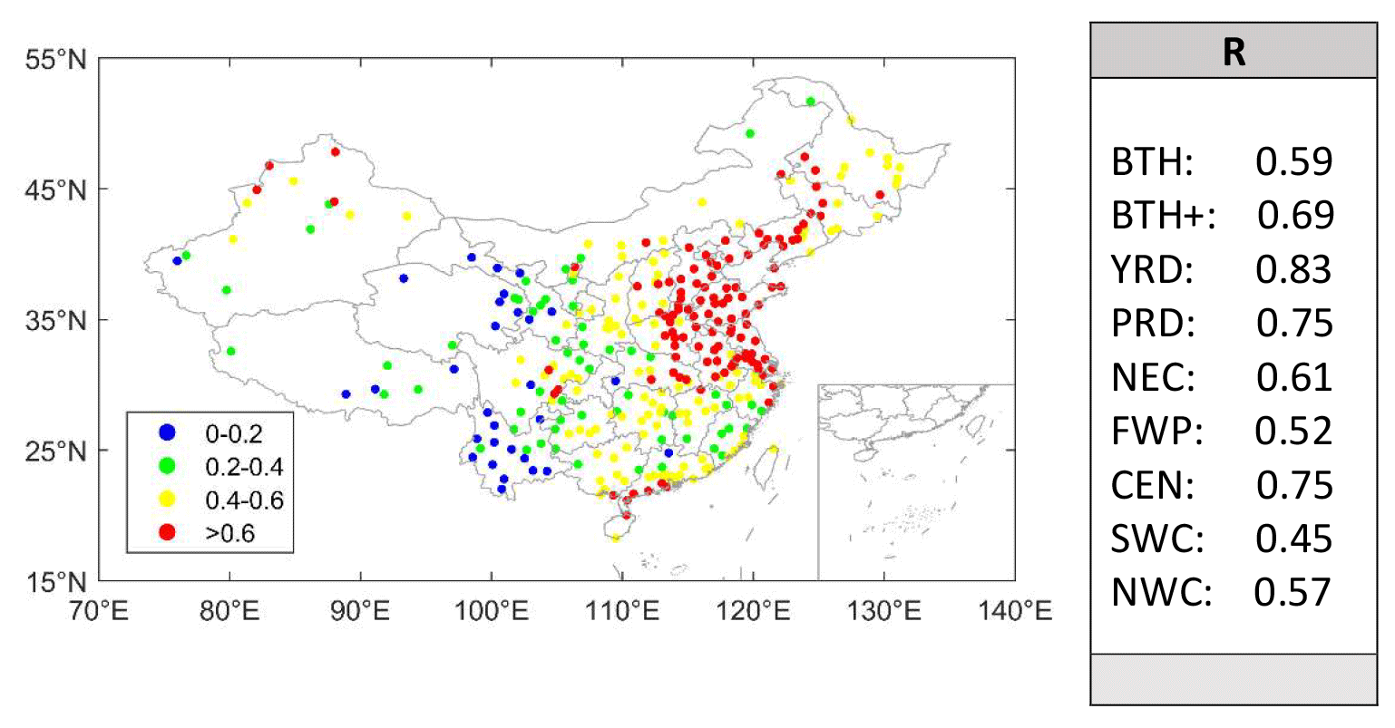
Figure 4 Correlation coefficients (R) between the EMI_2.5 and the observed PM_2.5 daily concentrations across China for 2017 and for typical regions averaged between 2013 and 2019.

To evaluate the applicability of EMI_2.5, the index was compared with the observed PM_2.5 concentrations. Figure 4 shows the spatial distribution of correlation coefficients between PM_2.5 and EMI_2.5 for 2017 for all of China. The correlation coefficients between EMI_2.5 and PM_2.5 concentrations are greater than 0.4 for most of eastern China and greater than 0.6 for most of the assessment regions. Less satisfactory correlation was found in western China, possibly due to complex terrain and less accurate emission data over there. Furthermore, due to the uncertainty in emissions and the difference in model performance for year-to-year meteorology simulations, the correlation coefficients may differ for different years. Overall, the good correlation between them merits the application of EMI_2.5 to quantify the meteorology impact on PM_2.5.

To further illustrate the applicability of EMI_2.5, the difference of various conditions between December 2014 and December 2015 in the BTH region was also analyzed when a significant change in air quality and meteorological conditions occurred. The winter of 2015 was accompanied by a strong El Niño (ENSO) event, resulting in significant anomalies for meteorological conditions in China. Analysis shows that the meteorological conditions in December 2015 (compared to December 2014) had several important anomalies, including that the surface southeasterly winds were significantly enhanced in the North China Plain (NCP) and the wind speeds were decreased in the middle north of eastern China and slightly increased in the south of eastern China. A study suggests that the 2015 El Niño event had significant effects on air pollution in eastern China, especially in the NCP region, including the capital city of Beijing, in which aerosol pollution was significantly enhanced in the already heavily polluted capital city of China (Chang et al., 2016).

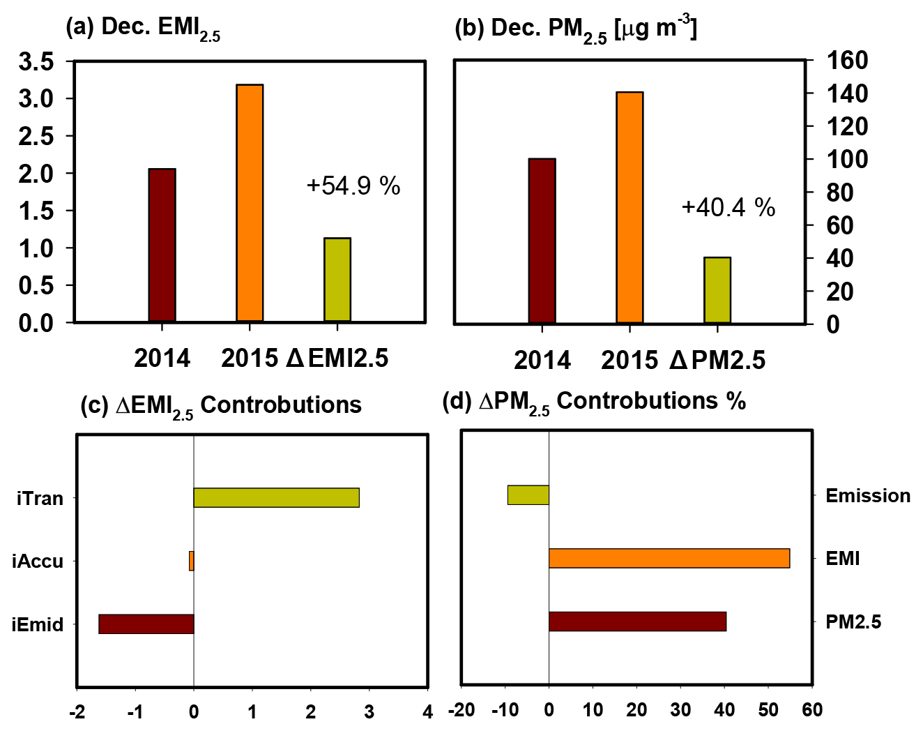
Figure 5 (a) The monthly averaged EMI_2.5 and (b) monthly PM_2.5 for the Decembers of 2014 and 2015 over BTH. (c) Contributions of the sub-index to the EMI_2.5 change and (d) contributions of emission and meteorology changes to PM_2.5 change for the Decembers from 2014 to 2015, respectively.

Figure 5 shows the monthly average EMI_2.5, PM_2.5 and contribution of the sub-index to total EMI_2.5 in December 2014 and 2015 over the BTH region. The monthly average EMI_2.5 increases by about 54.9 % from 2.1 in December 2014 to 3.2 in December 2015, indicating worsening meteorological conditions for PM_2.5 pollution. The increase in EMI_2.5 is mainly contributed by adverse atmospheric transport conditions (Fig. 5c), which results in the increase in EMI_2.5 reaching 3.2. With the increase in background concentration, the deposition and vertical diffusion also increase and offset the impact of adverse transport conditions to some extent.

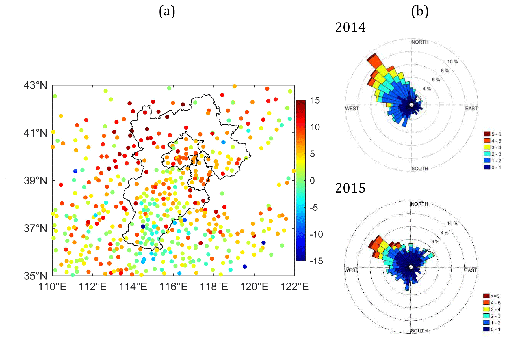
Figure 6 (a) The change in DSW (days) from December 2014 to December 2015 (December 2015–December 2014) and (b) wind rose maps in December 2014 and December 2015 over the BTH region.

The worsening meteorological conditions represented by EMI_2.5 were also supported by the observations for the two periods. The observed day with DSW, wind speed less than 2 m s⁻¹) reveals that, except for part of southern Hebei Province, the DSW increases by 5–15 d for 2015 in most meteorological stations in the BTH region (Fig. 6a), which indicates a large decrease in local diffusion capability. The comparison of the wind rose map shows that the decrease in northwesterly wind and the increase in southwesterly and northeasterly wind occurred in December 2015 (Fig. 6b). The change in wind fields indicates more pollutants were transported to the BTH region from Shandong, Jiangsu, Henan, and Northeast China. These variations indirectly validate the conclusions of adverse atmospheric transport conditions with high iTran in December 2015.

Based on the assessment method of emission contribution to the observed trend (Eqs. 6 and 7), the emission reduction in December 2015 as compared to 2014 was estimated to contribute about 9.4 % (Fig. 5d) to the PM_2.5 concentration decrease, compensating for the large increase caused by meteorology, which is comparable with previous studies of about 8.6 % reduction in emissions (Liu et al., 2017; He et al., 2017a) for the same 2 months. In other words, without the regional emission reduction efforts, the observed PM_2.5 concentration in December 2015 would have had a similar rate of 54.9 % increase to the worsening meteorology conditions as compared with December 2014. This assessment of emission reduction is supported by the estimate of emission inventories for the BTH region in the Decembers of 2014 and 2015 by Zheng et al. (2019), who found out that the monthly emission strengths for PM_2.5, SO₂, NO_x, VOCs and NH₃ in 2015 were reduced by 22.0 %, 6.9 %, 2.5 %, 2.5 % and 2.5 %, respectively, as compared with 2014. The sensitivity and the nonlinear response of PM_2.5 concentrations to the air pollutant emission reduction in the BTH region (Zhao et al., 2017) have been estimated to be about 0.43 for both primary inorganic and organic PM_2.5, 0.05 for SO₂, −0.07 for NO_x, 0.15 for VOCs, and 0.1 for NH₃. Combining the emission reduction percentages between the Decembers of 2014 and 2015 and the nonlinear response of emissions to the PM_2.5 concentrations results in an approximately 10.2 % ambient PM_2.5 concentration reduction due to the emission changes. This is very close to the estimate of emission reduction contribution to the December PM_2.5 concentration difference of about 9.4 % between 2014 and 2015 by the EMI framework.

Table 2 Comparison of PM_2.5 concentrations in the Novembers of 2017 and 2018 from ambient observations and from CTM simulations by EMI-derived estimated emission changes. The emission ratio is indicated by bold font and the two concentration ratios are in bold italic font.

The applicability of the EMI to assess the meteorology and emission changes is also evaluated by results from a full chemical transport model (MM5/CUACE) and observational data for PM_2.5 in China for the Novembers of 2017 and 2018. The averaged EMI_2.5 and observational data for the 2 months were used to estimate the emission change ratio (E-Ratio in Table 2) by Eqs. (6)–(7) from 2017 to 2018. In order to evaluate the correctness of this emission change estimate, the E-Ratio was used to adjust the emissions for November 2018 from the base emissions of the same month for 2017, which were then implemented in the MM5/CUACE to simulate the PM_2.5 concentrations for the 2 months, respectively. If the simulated concentration differences (M-Ratio) for the 2 months were comparable with the observed concentration differences (O-Ratio), it can be concluded that the emission change estimated by the EMI framework was reliable and could approximately represent the actual emission changes. Table 2 summarizes the analysis results of this evaluation for six typical cities. It is clear that the O-Ratios for the six cities are very comparable with M-Ratios, indicating that the EMI framework can be reasonably used to estimate the emission changes over time.

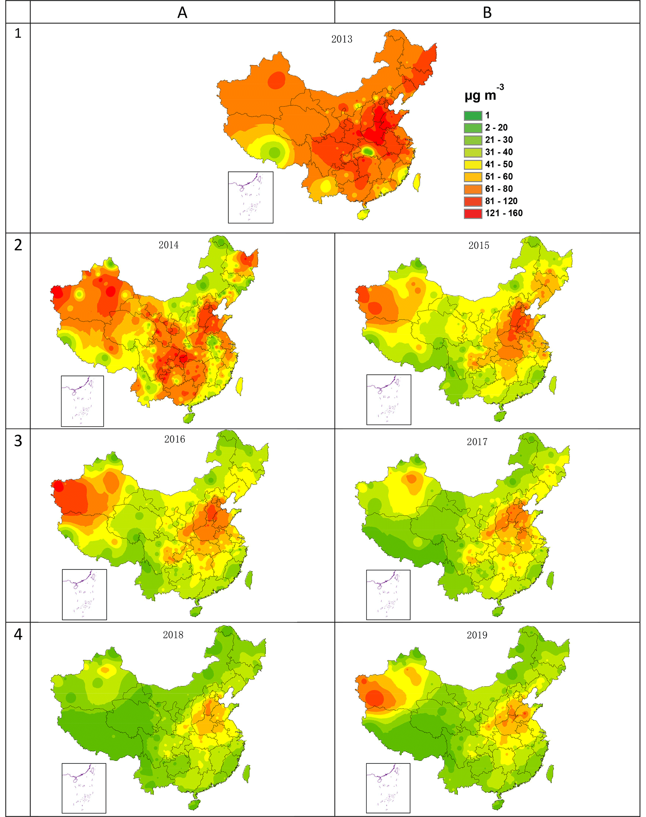
Figure 7 Regional annual PM_2.5 concentration distributions from 2013 to 2019.

3.2 PM_2.5 trends and meteorological contributions

The annual averaged PM_2.5 concentrations in China have been decreased significantly from 2013 to 2019. Figure 7 shows the observed spatial distribution of national PM_2.5 concentrations from 2013 to 2019, respectively. These spatial distributions are consistent with those of primary and precursor emissions of PM_2.5 (Wang et al., 2011), pointing out the fundamental cause of the air pollution in China. From the spatial distributions, it is clear that the regions of BTH, FWP, CEN and NWC had the highest PM_2.5 concentrations among the nine regions. Even though the national concentrations have been reduced significantly from 2013 by reducing emissions, the pollution center of particular matters has not been changed very much, located in southern Hebei Province and indicating the macroeconomic structure has not gone through a great change yet. Another phenomenon that can be seen from the distribution is that in Northwest China, especially in some cities of Xinjiang and Ningxia provinces, the PM_2.5 concentrations were on an increasing trend, due to certain migrating industries from developed regions in East China.

Averaged for the nation, nine focused regions and Beijing, the PM_2.5 trend lines were shown in Fig. 2. It is seen that all regions have had a large reduction of more than 35 % in surface PM_2.5 concentrations in 2019 as compared with those in 2013. The averaged national annual concentration at 36 µg m⁻³ has been very close to the national standard of 35 µg m⁻³, while the concentrations in the PRD, SWC and NEC regions have been below the standard. Regions above the standard are BTH+, BTH, YRD, CEN and FWP. Regionally, the largest drop percentage of PM_2.5 was seen in the NEC and NWC regions (Fig. 8), reaching over 50 % compared with 2013. In the BTH, BTH+, FWP and CEN regions, the reduction was in the range of 45 % to 50 %, while in YRD and PRD the reduction was around 35 %.

Figure 8 Annual averaged PM_2.5 concentrations in 2013 (a) and corresponding changing rates (b) from 2014 to 2019 as compared with 2013 for the nation, nine regions and Beijing.

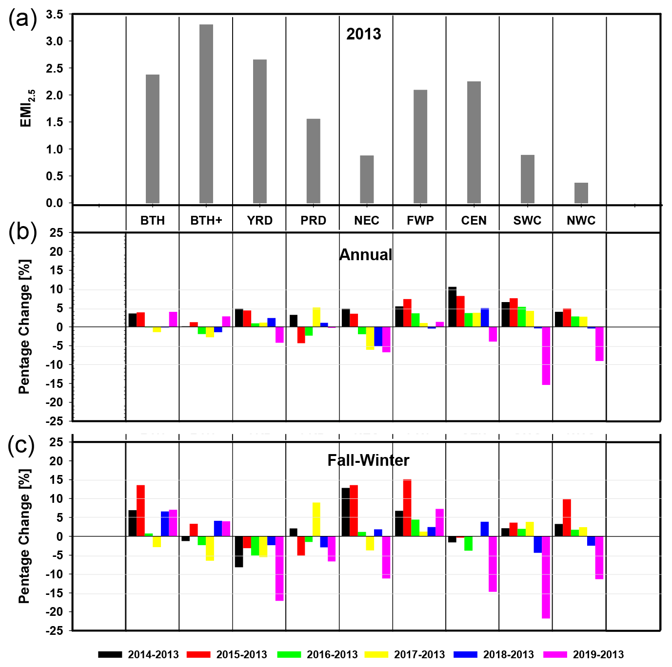
Figure 9 Annual averaged EMI_2.5 in 2013 (a) and corresponding changing rates for the annual average (b) and for the fall–winter seasons (c) from 2014 to 2019 as compared with 2013 in nine regions.

As one of the key factors in controlling the ambient PM_2.5 concentration variations, the annual meteorological fluctuations, i.e., EMI_2.5, from 2014 to 2019 with 2013 as the base year, are shown in Fig. 9 for nine regions. Generally, the annual EMI_2.5 shows a positive or negative variation, reflecting the meteorological features for that specific region. Except for a couple of regions or years, most of the fluctuations are within 5 % as compared with 2013 and have no definite trend. It can be inferred that the meteorological conditions are possibly responsible for about 5 % of the annual PM_2.5 averaged concentration fluctuations from 2013 to 2019 (Fig. 9b). This is consistent with what has been assessed in Europe by Andersson et al. (2007).

The variations in meteorological contributions (EMI_2.5) to PM_2.5 for the heavy pollution seasons of fall and winter (1 October to 31 March) generally follow the same fluctuating pattern as the annual average but are much larger than the average (Fig. 9c), over 5 % for most of the regions and years. For specific regions and years, e.g., BTH, YRD, NEC, SWC and CEN, the variations are between 10 % and 20 % as compared with 2013. Since the PM_2.5 concentrations are much higher in the pollution season, the larger meteorology variations in fall–winter would exercise more controls on the heavy pollution episodes than the annual averaged concentrations, signifying the importance of meteorology in regulating the winter pollution situations.

It is found that though most of the regions have a fluctuating EMI_2.5 in the pollution season during the 2014–2019 period (Fig. 9c), the YRD and FWP show consistent favorite and unfavorite meteorological conditions, respectively. BTH has witnessed the same unfavorite conditions as FWP, except in 2017. In other words, in BTH and FWP, the decrease in ambient concentrations of PM_2.5 from 2014 to 2019 has to overcome the difficulty of worsening meteorological conditions with larger control efforts.

3.3 Attribution of control measures to the PM_2.5 trend

As it is well known that the final ambient concentrations of any pollutants result from the emission, meteorology and atmospheric physical and chemical processes, separating emissions and meteorology contributions to the pollution-level reduction entails a combined analysis of them. The analysis in Sect. 3.2 shows that from 2013 to 2019, the national averaged PM_2.5 as well as those for nine separate regions were all showing a gradual decline trend (Fig. 8). By 2019, 45 %–50 % of reductions in surface PM_2.5 concentrations were achieved, while the meteorology contributions did not show a definite trend as from 2013, clearly pointing out the contribution of emission reductions in the trend. Using the analysis framework for separating emissions from meteorology based on the monitoring data of PM_2.5 and EMI_2.5 (Sect. 2.4), the emission change contributions are estimated.

Figure 10 Annual PM_2.5 emissions (total and per unit km²) for 2013 (a) and corresponding changing rates (b) from 2014 to 2019 as compared with 2013 in nine regions.

Table 3 Observed PM_2.5 difference between 2019 and 2015 as well as its attributions to meteorology and control measures for all of China, Beijing and nine regions.

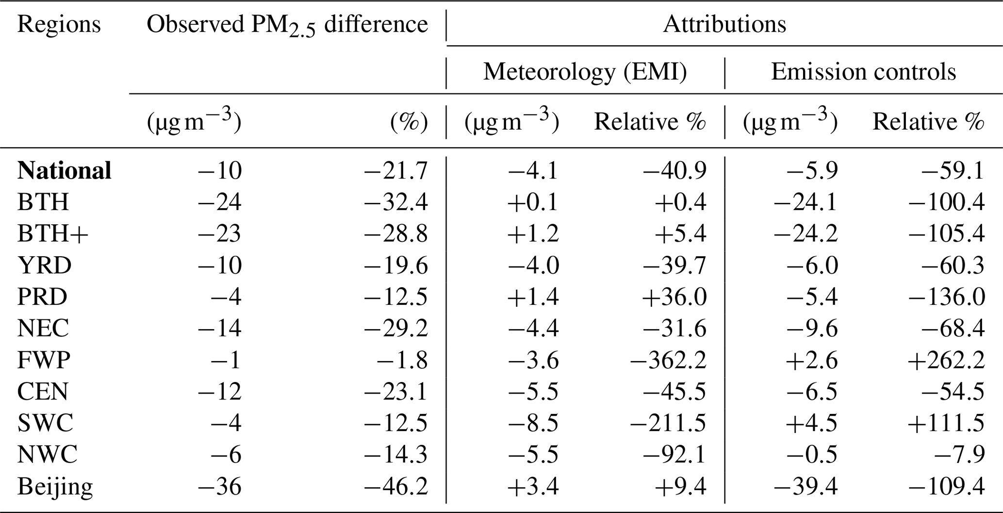
Note: “+” increased; “−” decreased.

Figure 10 shows the 2013 base emissions of PM_2.5 (Zhao et al., 2017) and the annual changes in the emission contributions to the PM_2.5 concentrations from 2014 to 2019 as estimated from the EMI_2.5 and observed PM_2.5. For the emissions, it is found that the unit area emissions match better with ambient concentrations of PM_2.5 in regions than the total emissions and the high-emission regions are BTH, BTH+, YRD, PRD and FWP in 2013. Nationally by 2019, the emission reduction contributions to the ambient PM_2.5 trend ranged from 32 % to 52 % of the total PM_2.5 decrease percentage, while in the BTH and BTH+ regions the reduction was more than 49 % from the 2013 base year emissions, leading the national emission reduction campaign. The emission reduction rates clearly illustrate the effectiveness of the nationwide emission control strategies implemented since 2013, and the emission reduction is the dominant factor for the ambient PM_2.5 declining trend in China. Taking the analysis data of PM_2.5 and EMI_2.5 from this study for the BTH+ region from 2013 to 2017, it is found that the control strategy contributed more than 90 % to the PM_2.5 decline. Chen et al. (2019) estimated that the control of anthropogenic emissions contributed 80 % of the decrease in PM_2.5 concentrations in Beijing from 2013 to 2017.

Regionally, the emission reduction trends from 2014 to 2019 display some unique characteristics. For the regions of BTH, BTH+ and PRD, the year-by-year reduction rate is consistent, indicating that regardless of fluctuations in meteorology, these regions have had an effective emission control strategy and maintained the emission reduced year by year since 2014. However, in some regions such as FWP, NEC, SWC and NWC, the emission reduction rates were fluctuating from 2014 to 2019, implying that the emissions in these regions were increased in certain years. Especially in FWP from 2016 to 2017, the emissions were estimated to be increased by about 10 % and then decreased in 2018 and 2019, despite the fact that FWP experienced unfavorite meteorological conditions during this period.

The year of 2015 is a special year in the history of China air pollution control. Though the systematical and network observations of PM_2.5 started in China from 2013, it took about 2 years (until 2015) to evolve to the current status in terms of spatial coverage and observational station numbers, establishing a consistent and statistically comparable national network. In the same year, the Environmental Protection Law of the People's Republic of China took effect in January, signalizing the stage of lawful control of air pollution. From the regulation assessment point of view, the impact by emission changes from 2015 was relevant to the interests of management to show how effective the law was.

Table 3 summarizes the PM_2.5 difference between 2019 and 2015 and the relative contributions of meteorology and emission changes to the difference for all of China, Beijing and nine regions. Once again, as of the end of 2019, the PM_2.5 concentrations are all reduced from 2015, ranging from −1.8 % in FWP to −46.2 % in Beijing. During this period of time, regions of BTH, BTH+, PRD and Beijing had encountered unfavorite meteorological conditions with positive EMI_2.5 changes, which indicated that for these regions, emission reductions were not only to maintain the decline trend, but also to offset the unfavorite meteorological conditions in order to achieve the observed reductions in ambient PM_2.5 concentrations. By contrast, for the regions of FWP and SWC, the emission control impacts were to deteriorate the concentrations, implying an increase in emissions to restrain the PM_2.5 concentration decrease by favorite meteorological conditions. For other regions, both meteorology and emission controls contributed to PM_2.5 decrease from 2015 to 2019, with the control measures contributing −7.9 % in NWC to −68.4 % in NEC (Table 3).

Therefore, due to the diversity of meteorological conditions and emission distributions in China, their impacts on ambient PM_2.5 concentrations display unique regional characteristics. Overall, the emission controls are the dominant factor in contributing the declining trend in China from 2013 to 2019. However, in certain regions or certain periods of years, emissions were found to be increased even with favorite meteorological conditions, which means the design of national control strategies has to take both meteorology and emission impacts simultaneously in order to achieve maximum results.

4 Conclusions

Based on a 3-D chemical transport model and its process analysis, an Environmental Meteorological Index (EMI_2.5) and an assessment framework have been developed and applied to the analysis of the PM_2.5 trend in China from 2013 to 2019. Compared with observations, the EMI_2.5 can realistically reflect the contribution of meteorological factors to the PM_2.5 variations in the time series with impact mechanisms and can be used as an index to judge whether the meteorological conditions are favored or not for the PM_2.5 pollutions in a region or time period. In conjunction with the observational trend data, the EMI_2.5-based framework has been used to quantitatively assess the separate contribution of meteorology and emission changes to the time series for nine regions in China. Results show that for the period of 2013 to 2019, the PM_2.5 concentrations dropped continuously throughout China, by about 50 % on the national average. In the regions of NWC, NEC, BTH, BEIJING, CEN, BTH+, and SWC, the reduction was in the range of 46 % to 53 %, while in FWP, PRD, and YRD, the reduction was from 45 % to 35 %. It is found that the control measures of emission reduction are the dominant factors in the PM_2.5 declining trends in various regions. By 2019, the emission reduction contributes about 47 % of the PM_2.5 decrease from 2013 to 2019 on the national average, while in the BTH region the emission reduction contributes more than 50 %, and in the YRD, PRD, and SWC regions, the contributions were between 32 % and 37 %. For most of the regions, the emission reduction trend was consistent throughout the period except for FWP, NEC, SWC, and NWC, where the emission amounts were increased for certain years. The contribution by the meteorology to the surface PM_2.5 concentrations from 2013 to 2019 was not found to show a consistent trend, fluctuating positively or negatively about 5 % on the annual average and 10 %–20 % for the fall–winter heavy-pollution seasons. It is noted that the estimate of emission control contributions was made under a first-order approximation of emission and meteorology, which should be improved in the future implementations.