Measurement report: characteristics of clear-day convective boundary layer and associated entrainment zone as observed by a ground-based polarization lidar over Wuhan (30.5° N, 114.4° E)

Knowledge of the convective boundary layer (CBL) and associated entrainment zone (EZ) is important for understanding land–atmosphere interactions and assessing the living conditions in the biosphere. A tilted 532 nm polarization lidar (30^∘ off zenith) has been used for the routine atmospheric measurements with 10 s time and 6.5 m height resolution over Wuhan (30.5^∘ N, 114.4^∘ E). From lidar-retrieved aerosol backscatter, instantaneous atmospheric boundary layer (ABL) depths are obtained using the logarithm gradient method and Harr wavelet transform method, while hourly mean ABL depths are obtained using the variance method. A new approach utilizing the full width at half maximum of the variance profile of aerosol backscatter ratio fluctuations is proposed to determine the entrainment zone thickness (EZT). Four typical clear-day observational cases in different seasons are presented. The CBL evolution is described and studied in four developing stages (formation, growth, quasi-stationary and decay); the instantaneous CBL depths exhibited different fluctuation magnitudes in the four stages and fluctuations at the growth stage were generally larger. The EZT is investigated for the same statistical time interval of 09:00–19:00 LT. It is found that the winter and late autumn cases had an overall smaller mean (mean) and standard deviation (SD) of EZT data compared to those of the late spring and early autumn cases. This statistical conclusion was also true for each of the four developing stages. In addition, compared to those of the late spring and early autumn cases, the winter and late autumn cases had larger percentages of EZT falling into the subranges of 0–50 m but smaller percentages of EZT falling into the subranges of > 150 m. It seems that both the EZT statistics (mean and SD) and percentage of larger EZT values provide measures of entrainment intensity. Common statistical characteristics also existed. All four cases showed moderate variations of the mean of the EZT from stage to stage. The growth stage always had the largest mean and SD of the EZT and the quasi-stationary stage usually the smallest SD of the EZT. For all four stages, most EZT values fell into the 50–150 m subrange; the overall percentage of the EZT falling into the 50–150 m subrange between 09:00 and 19:00 LT was > 67 % for all four cases. We believe that the lidar-derived characteristics of the clear-day CBL and associated EZ can contribute to improving our understanding of the structures and variations of the CBL as well as providing a quantitatively observational basis for EZ parameterization in numerical models.

1 Introduction

Monitoring the atmospheric boundary layer (ABL) is of essential importance, since the ABL is in direct contact with nearly all terrestrial life on earth (Lammert et al., 2006). The ABL is located in the lower part of the troposphere and is subjected to influences of various processes. These processes, including land or water surface exchanges at the bottom and entrainments at the top, govern the transport of heat, momentum, moisture and substances (e.g., aerosols and other constituents) between the ground and the free atmosphere (FA) (Stull, 1988; Pal et al., 2010).

The depth (or height) of the ABL is a key parameter for parameterization of the ABL, as it determines the available volume for pollutants dispersion and resulting concentrations (Pal et al., 2015; Li et al., 2017; Su et al., 2018, 2020) as well as the regional dimension in which transport processes can take place. The ABL depth is defined as the interfacial height that separates the ABL and the FA (Stull, 1988). It actually exhibits apparent diurnal evolution following the local surface temperature variation with a magnitude ranging from a few tens of meters to several kilometers (Kong and Yi, 2015). In clear daytime after sunrise, the ABL depth generally increases first as convective activities intensify, then decreases after reaching its maximum in the afternoon when turbulence intensity decays. The convectively driven ABL is designated as the convective boundary layer (CBL). After sunset, the CBL is replaced by the stable boundary layer (SBL; or nocturnal boundary layer, NBL) with a much lower depth. Because the convective processes driven by the sensible heat flux at the surface can be reflected by tracers (e.g., water vapor and aerosols) concentration within the CBL and in various atmospheric variables, multiple methods based on tracers and distinct instrumentations have been utilized to determine the CBL depth (Behrendt et al., 2011a; Cimini et al., 2013; Sawyer and Li, 2013). In situ radiosonde measurements serve as one popular way to derive CBL depth (Seidel et al., 2010; Guo et al., 2019) for its wide distribution all over the world and long observation history, which makes it suitable for CBL depth climatology studies (Dang et al., 2019) despite its low temporal resolution (usually 2–4 times per day). From radiosonde profiles of temperature, pressure, humidity and wind, the CBL depth can be retrieved using the parcel method (Hennemuth and Lammert, 2006; Seidel et al., 2010), Richardson method (Seibert et al., 2000; Seidel et al., 2010; Zhang et al., 2013), and gradient method (Seidel et al., 2010). Ground-based remote sensing instruments, such as sodar (Helmis et al., 2012), microwave radiometer (Cimini et al., 2013), wind profiling radar (Liu et al., 2019), ceilometer (Zhu, 2018) and lidar, favor continuous monitoring of the CBL depth at a fixed location; space-borne lidar like Cloud–Aerosol Lidar with Orthogonal Polarization (CALIOP), on the other hand, can provide global coverage but suffers from a low signal-to-noise ratio (SNR) at daytime for CBL measurements (Liu et al., 2015; Zhang et al., 2016; Su et al., 2017). Among these remote sensing techniques, lidar can continuously measure the atmospheric backscatter with high spatial and temporal resolution, which thus enables detailed study on the small-scale structures in the CBL. Based on the lidar-derived backscatter information from given trace substances (e.g., water vapor and aerosols), the ABL depth can be determined by using either the process-based variance method (e.g., Lammert et al., 2006; Martucci et al., 2007; Wulfmeyer et al., 2010; Pal et al., 2013; Kong and Yi, 2015) or vertical-distribution-based method (e.g., the derivative method, the Harr wavelet transform method) (Cohn and Angevine, 2000; Brooks, 2003; Morille et al., 2007; Baars et al., 2008; Pal et al., 2010; Granados-Muñoz et al., 2012; Lewis et al., 2013; Sawyer and Li, 2013; Su et al., 2020). Recently, multiple-methods-based algorithms as mentioned above have been developed and are capable of yielding robust and accurate determination of CBL depth objectively (e.g., Pal et al., 2013; Dang et al., 2019).

Turbulence is a frequent phenomenon in the CBL and turbulent mixing serves as an effective mechanism resulting in homogeneous distribution of scalars (e.g., humidity, aerosols and other constituents) in the middle and lower parts of the CBL (Manninen et al., 2018). The middle and lower parts of the CBL characterized by even mixing is also called the mixing layer (ML). However, near the top area of the CBL, a sharp gradient of scalars might appear due to vigorous mixing of overshooting thermals (updrafts) and FA air (downdrafts) (Stull, 1988). This region corresponds to the entrainment zone (EZ). Entrainment processes that occur in the EZ control CBL growth and structure as well as cloud formation and distribution in the CBL (Brooks and Fowler, 2007). Entrainment rate is an important parameter for understanding the fundamental physical entrainment processes; however, this parameter cannot be directly measured and instead needs to be inferred from other measurement results (Lenschow et al., 1999). The entrainment zone thickness (EZT) provides a possibility for parameterizing the entrainment rate (Deardorff et al., 1980). The top of the EZ can be regarded as the highest height that the thermal reaches within a region (Stull, 1988), while the bottom of the EZ is difficult to define and is usually taken subjectively as the height where about 5 %–10 % of the air on a horizontal plane has the FA characteristics (e.g., Deardorff et al., 1980; Wilde et al., 1985). The EZT is hence determined by the top and bottom heights of the EZ and reflects the recent mixing history driven mainly by the small-scale turbulent processes responsible for entrainment (Davis et al., 1997). Since small-scale processes often become important in the EZ due to high variability of the scalar distribution in these regions, determination of the EZT requires the monitoring of tracers with very high temporal–spatial resolution in this area. Based on high-resolution time series of the instantaneous ABL depth retrieved by lidar or wind profiling radar, the standard deviation technique (e.g., Davis et al., 1997) and the cumulative frequency distribution method (e.g., Wilde et al., 1985; Flamant et al., 1997; Pal et al., 2010; Cohn and Angevine, 2000) have been employed to investigate the EZT. However, the above two methods yield EZT values with large differences (e.g., Pal et al., 2010); the choice of specific percentages of air having the FA characteristics for the definition of EZ bottom height varies (between 5 % and 15 %) among researchers (e.g., Deardorff et al., 1980; Wilde et al., 1985; Flamant et al., 1997; Cohn and Angevine, 2000; Pal et al., 2010). Moreover, considering that variations of ABL depths can result not only from entrainment but also non-turbulent processes (e.g., atmospheric gravity waves and mesoscale variations in the ABL structure), the methods depending on variations of ABL depth might not really characterize the true EZ (Davis et al., 1997). So far, no universally accepted approach exists for the determination of the EZT (Brooks and Fowler, 2007).

Currently, studies are generally concentrated on the CBL and relatively rarely on the EZ. The basic physical processes governing entrainment and their relationship with other boundary layer properties are still not fully understood (Brooks and Fowler, 2007). In addition, the general grid increments of state-of-the-art weather forecast and climate models are too coarse to resolve small-scale boundary layer turbulence (Wulfmeyer et al., 2016). Therefore, continuous and high-resolution measurements at various observational locations to infer detailed knowledge of both the CBL and associated EZ, especially small-scale boundary layer turbulence therein, are of significant importance to boundary layer studies including land–atmosphere interactions, air quality forecasts, and almost all weather and climate models (Wulfmeyer et al., 2016). In this work we present the high-resolution measurement results of the CBL and associated EZ using a recently developed titled polarization lidar (TPL) over Wuhan (30.5^∘ N, 114.4^∘ E). The TPL is housed in a customized working container and capable of operating under various weather conditions (including heavy precipitation). The TPL has an inclined working angle of 30^∘ off zenith and routinely monitors the atmosphere with a time resolution of 10 s and a height resolution of 6.5 m. The equivalent minimum height with full overlap for the TPL is ∼ 173 m a.g.l. (above ground level). Based on the TPL-measured backscatter, a new approach has been developed for determining the EZT. The small-scale characteristics of the CBL and associated EZ have also been investigated, which can contribute to the improvement of understanding the structures and variations of the ABL, as well as parameterization of the EZ. The instrument, methodology and observational results are described and a summary and conclusions are presented in the following sections.

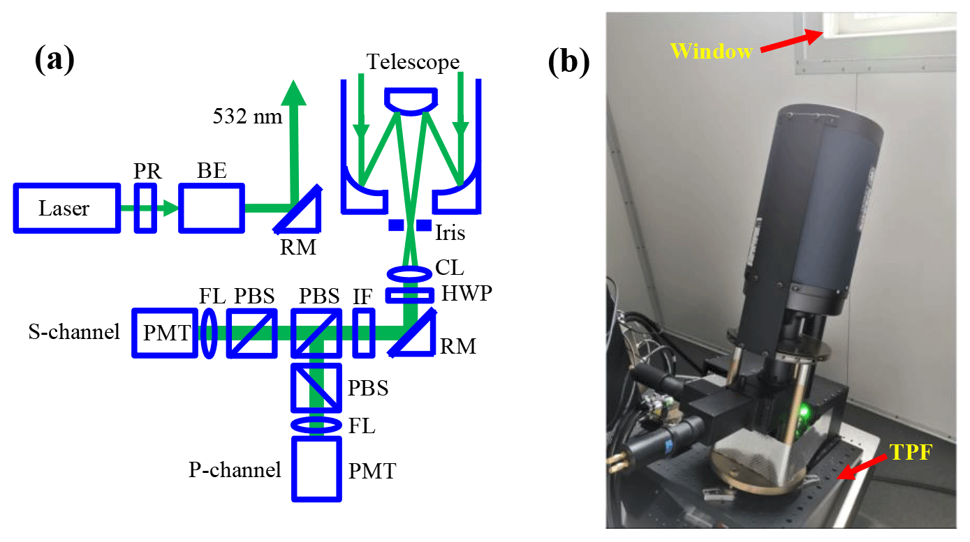
Figure 1 (a) Schematic optical layout of the TPL. PR, polarizer, beam expander (BE), reflecting mirror (RM), collimating lens (CL), half-wavelength plate (HWP), interference filter (IF), polarization beam splitter (PBS), focusing lens (FL) and photomultiplier tube (PMT). (b) A picture of the lidar optics. The whole optics is placed on a tilted platform (TPF). A window permits the propagating laser beam and atmospheric backscatter to pass through without being blocked.

2 Instrument

The TPL is located on the campus of Wuhan University, Wuhan, China (30.5^∘ N, 114.4^∘ E and 70 m a.s.l.). Figure 1a shows a schematic optical layout of the lidar system. The lidar transmitter introduces a solid Nd:YAG laser to generate an emission of 70 mJ per pulse at 532 nm with a repetition of 20 Hz. A Brewster polarizer (PR) improves the linear polarization purity of the outgoing laser light before entering the beam expander (BE). The 3 × BE compresses the divergence of the laser to be < 0.25 mrad. A steerable reflecting mirror (RM) then guides the expanded beam into the atmosphere. In the receiver, a Cassegrain telescope collets the atmospheric backscatter. The telescope has a clear aperture of 203.2 mm and a focal length of 2032 mm. The subsequent optics contains an iris, a collimating lens (CL), a half-wavelength plate (HWP), a RM and an interference filter (IF). The iris sets the telescope field of view to be 1.0 mrad. The HWP guarantees the polarization plane of the propagating light beam to be exactly coincident with the receiver polarization analyzer. The IF has a bandwidth of 0.17 nm centered at 532 nm and a peak transmittance of 79 %. After being filtered by the IF, the parallel and perpendicular polarization light components are detected by two detection channels (designated as the P- and S-channel, respectively). In each of the P- and S-channels, two cubic polarization beam splitters (PBS) are cascaded to reduce crosstalk between the two orthogonal polarization channels. A focusing lens (FL) then focuses the signal light on the photosensitive surface of the subsequent photomultiplier tube (PMT); neutral density filters (not shown here) are also added before the FL to avoid saturation of the PMT. Finally, a PC-controlled two-channel transient digitizer (TR20-160, Licel) records the detected signals as raw saved data with a time resolution of 10 s and range resolution of 7.5 m.

Figure 1b provides a picture of the TPL transmitting–receiving optics. The whole optics is installed on a mechanical tilted platform (TPF) which is fixed with an elevation angle of 30º. Since the telescope is located with its optical axis perpendicular to the TPF top surface, this translates a same angle of 30º for the telescope optical axis off zenith. In addition, the TPL system is housed in a customized working container with temperature and humidity control. The working container has a window on one side that opens to permit the propagating laser beam and atmospheric backscatter to pass through without being blocked. The working container enables the TPL to operate under various weather conditions including heavy precipitation.

The whole transmitting–receiving optics of the TPL has a compact arrangement and the tested minimum range with full overlap is 200 m. Given the 30^∘ tilted angle off zenith, this yields an equivalent height of ∼ 173 m a.g.l. Thus the TPL partly provides a possibility for the depth investigation of shallow CBL and NBL. The channel gain ratio of the TPL was calibrated after its foundation using the sky background method (Wang et al., 2009). Specifically, the calibration was performed when the sky was clouded over so that the background sun light could be regarded as totally unpolarized. The gain ratio turned out to be 0.09521 ± 0.00031. It is further investigated that the lidar-measured molecular volume depolarization δ_V,m in clear areas is 0.00780 ± 0.00072. Considering that the theoretical δ_V,m for this TPL should be 0.00364 (Behrendt et al., 2002), the offset value of 0.00416 due to depolarization effect of the lidar system is rather small and thus neglected.

3 Methodology

3.1 Method to determine ABL depth

The Licel-recorded raw analog and photon count data are first used to generate a reasonable photon count profile with a larger dynamic range based on a developed gluing algorithm (Newsom et al., 2009; Zhang et al., 2014). This glued photon count profile retains a temporal resolution of 10 s and a range resolution of 7.5 m. Combining the obtained P- and S-channel signals, the unpolarized range-square corrected elastic signal X at range R can be reconstructed by

$$\begin{array}{}\text{(1)}& X\left(R\right)=[N_{\text{p}}\left(R\right)+\text{GR}\times N_{\text{s}}\left(R\right)]\times R^{\mathrm{2}},\end{array}$$

where the subscripts p and s denote the P- and S-channel, respectively. N is the background-subtracted photon count signal. The channel gain ratio GR has already been determined as stated before.

Since the TPL is slantingly pointed with an angle of 30^∘ off zenith, the range R can be readily converted to the corresponding height z by multiplying a factor of cos 30^∘. Hereafter in this work we use height z instead of range R. From the range-square corrected elastic signal X, the vertical-distribution-based method can be employed to determine an ABL depth for each X profile. Here both the logarithm gradient method (LGM) (e.g., Wulfmeyer, 1999; Pal et al., 2010) and Harr wavelet transform method (HWT) (e.g., Davis et al., 2000; Brooks, 2003) are tested to retrieve ABL depth.

The ABL depth z_LGM determined using the LGM method is defined as

$$\begin{array}{}\text{(2)}& z_{\text{LGM}}=min\left[D\left(z\right)\right]=min\left[{\displaystyle \frac{d\ln X\left(z\right)}{\mathrm{d}z}}\right],\end{array}$$

where D stands for the derivative of logarithmic X.

The ABL depth z_HWT determined by using the HWT method is defined as

$$\begin{array}{}\text{(3)}& \begin{array}{c}{z}_{\text{HWT}}=max\left[W_{\text{f}}\left(a,b\right)\right]=max\left[\frac{\mathrm{1}}{a}{\int }_{z_{\text{min}}}^{z_{\text{max}}}X\left(z\right)H\left(\frac{z-b}{a}\right)\mathrm{d}z\right]\\ \text{for}{z}_{\text{min}}<b<z_{\text{max}}\\ \text{and}H\left(\frac{z-b}{a}\right)=\left\{\begin{array}{c}\mathrm{1},b-a/\mathrm{2}\le z\le b\\ -\mathrm{1},b<z\le b+a/\mathrm{2},\\ \mathrm{0},\text{elsewhere}\end{array}\right.\end{array}\end{array}$$

in which W_f is the covariance transform value and H is the Harr wavelet function. The dilation a is tested and set to be 200 m for this work. z_min and z_max are the lower and upper heights for the lidar signal profile, respectively.

The advantage of applying the LGM and HWT methods is that an instantaneous ABL depth can be determined according to each X profile, which favors a high temporal resolution. However, in the case of residual layer (RL) or multiple aerosol layers, several local minima usually occur for the retrieved D profile, making the choice of the true minimum for the LGM method difficult (Menut et al., 1999; Pal at al., 2010). As for the HWT method, when the ABL is shallow (e.g., for the NBL and the early stage of the CBL after sunrise) subjective constraints on the upper integral height z_max need to be made to the base of existing aerosol layers aloft (Gan et al., 2011). All these situations hinder the LGM and HWT methods from an automated and robust attribution of the ABL depth.

To find a more reliable method suitable for an automated procedure, the process-based variance method can be utilized to provide a reference for the search for a local minimum by using the LGM method or the search for a local maximum by using the HWT method in a given time interval (e.g., Lammert et al., 2006; Pal et al., 2013). In this work, the variance profile of aerosol backscatter ratio (ABR) fluctuations is calculated and the height with maximum variance is assigned as ABL depth. Here the ABR profile is retrieved using the Fernald backward iteration method given a fixed lidar ratio (Fernald, 1984; Behrendt et al., 2011b). The fixed lidar ratio is chosen to be 50 sr at 532 nm according to existing measurement results of urban aerosols (e.g., Ansmann et al., 2005; Müller et al., 2007). The typical time interval is 1 h for generating a variance profile. Note that this variance method determines a mean ABL depth for the given 1 h time interval. To attribute the instantaneous ABL depth in the same time interval, the height with local minimum or maximum by using the LGM or HWT method, respectively, nearest to the hourly mean ABL depth by using the variance method is selected.

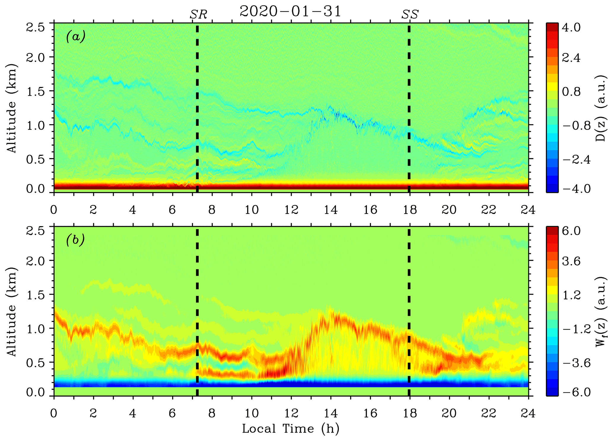
Figure 2 Contour plots of (a) D(z) and (b) W_f(z) on 31 January 2020. Sunrise (SR) and sunset (SS) times are marked by thick black dashed lines. Multiple (residual) aerosol layers that definitely lead to misattribution of ABL depth are clearly indicated by stripes of local minima of D(z) and maxima of W_f(z) in the contour plots. By visualizing these contour plots, proper upper heights for applying the variance method can be conveniently and correctly determined to be below the base of multiple (residual) aerosol layers aloft.

The remaining problem is that several local peaks might also appear for the variance profile in the case of multiple (residual) aerosol layers. This problem is solved by visualizing the contour plots of D(z) and W_f(z) to limit a proper height range for variance calculating. As an example, Fig. 2 shows the calculated D(z) and W_f(z) in the height range of 0–2.5 km on 31 January 2020. Sunrise (SR) and sunset (SS) times are marked by thick black dashed lines. As seen in Fig. 2, before 10:00 LT (local time), multiple (residual) aerosol layers above 0.5 km were clearly indicated by stripes of local minima of D(z) and maxima of W_f(z); in addition, advected aerosols above 0.7 km were also discernible after 19:30 LT (see also Fig. 4). From Fig. 2, it is noticed that an abundant aerosol layer subsided from around 1.25 km at 00:00 LT to about 0.6 km at 10:00 LT. This layer definitely leads to misattribution of the ABL depth by the automated procedure using the LGM and HWT methods as well as by the variance method. By visualizing these contour plots, it is intuitive and convenient to distinguish and locate the above misleading aerosol layers. Then, proper upper height limits for applying the variance method can be correctly determined, as the real ABL should be below these multiple (residual) aerosol layers aloft. At around 19:30 LT after SS, the subsided CBL near 0.6 km should be re-categorized as an RL. Again, the proper upper height limits for applying the variance method shall be set below the RL for the ABL (NBL) depth determination after 19:30 LT.

3.2 Method to determine the EZT

Since simultaneous measurement of the atmosphere in a large horizontal plane is actually difficult, an equivalent continuous sampling in the time domain at a fixed monitoring site is favored and can be easily performed given the Taylor's hypothesis of “frozen turbulence” theory (Stull, 1988). Under this assumption and from the retrieved time series of instantaneous ABL depth, the standard deviation technique (e.g., Davis et al., 1997) and the cumulative frequency distribution method (e.g., Wilde et al., 1985; Flamant et al., 1997; Pal et al., 2010) can be employed to obtain the EZT. However, the values of EZT obtained by using these two methods exhibit obvious discrepancies (e.g., Pal et al., 2010). The choice of specific percentage of air having the FA characteristics for the definition of EZ bottom height is rather subjective and seems variable among different researchers. Moreover, considering that variations of ABL depths can result not only from entrainment but also non-turbulent processes (e.g., atmospheric gravity waves and mesoscale variations in the ABL structure), the above methods might not really characterize the true EZ (Davis et al., 1997). This situation motivates us to develop a new approach to determine the EZT in this work.

The top and bottom heights of the EZ first given by Deardoff et al. (1980) and Wilde et al. (1985) have, respectively, 100 % and 5 %–10 % air on a horizontal plane sharing the FA characteristics. It is concluded that the top and bottom heights, especially the bottom one, are defined in a statistically averaged manner. Also, when observed from the perspective of physical process, entrainment mixing of clean FA air and well-mixed ML air generally results in significant fluctuations of scalars (e.g., number density of aerosols) in the EZ (see Figs. 4 and 7). In the absence of clouds and advected aerosols, the fluctuation magnitudes of aerosol number density in the EZ are usually larger than those in the FA and ML. Taking all of the above into consideration, the variance of ABR fluctuations is utilized here to statistically represent the fluctuations of aerosol number density. Subsequently, the full width at half maximum (FWHM) of the variance profile of ABR fluctuations can be employed to define the EZ, as this FWHM records the recent mixing history and quantitatively indicates in which area the larger variations of aerosol number density (ABR) takes place. In detail, the height with maximum variance in a variance profile calculated in a given time interval is first located as the ABL depth; this is coincident with the definition of the ABL depth by the variance method. Then, the upper and lower heights with half value of the maximum variance are searched for and defined as the top and bottom heights of EZ, respectively. Note that the FWHM of the variance profile of ABR fluctuations is utilized here because it physically represents that most aerosols have been strongly mixed in the vertical height interval defined according to the FWHM. The EZT is consequently determined by the height interval between the searched for top and bottom heights of EZ. This method is designated as the FWHM method here.

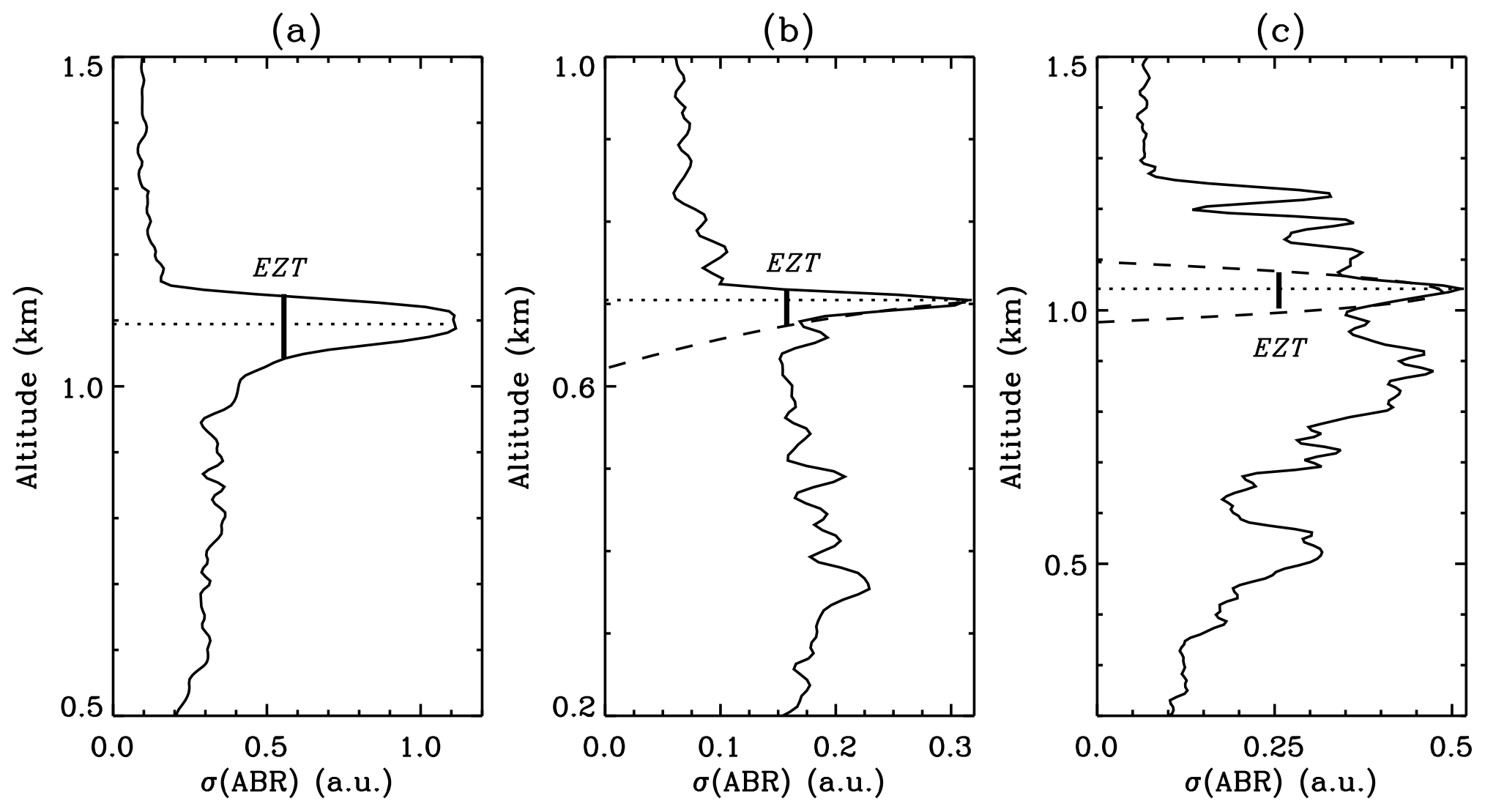
Figure 3 Illustrations of the FWHM method using the variance of ABR fluctuations to determine the CBL depth and subsequent EZT. Thin black lines indicate the standard deviation of ABR fluctuations, σ(ABR). Thin dotted lines specify the CBL depth with maximum σ(ABR). Thick vertical lines represent the determined EZT (EZ). (a) For a strong updraft case, both the upper and lower edges near the peak σ(ABR) are clear-cut and steep. The EZT can be directly obtained. (b) For a less-intense updraft case, the lower edge is not clear-cut enough. A quadratic polynomial fitting (dashed line) is applied to the lower edge to help determine the EZT. (c) For a weak turbulence and advected aerosol case, neither the upper nor the lower edge is clear-cut enough. Quadratic polynomial fittings (dashed lines) are applied to both edges to help determine the EZT.

As an example, Fig. 3 illustrates the FWHM method of using the variance of ABR fluctuations to determine the EZT. In Fig. 3a, the profile of the standard deviation of the ABR, σ(ABR), is first calculated for a chosen time interval and plotted as a thin black line. From this σ(ABR) profile, the CBL top (indicated by the dotted line) is definitely located at the height with maximum σ(ABR). For a strong updraft (as in this case) that carries ML air upward into the FA, intense fluctuations occur in the EZ while less-intense fluctuations in the ML and FA. Therefore, the corresponding σ(ABR) profile exhibits much larger values near the CBL depth as well as clear-cut steep upper and lower edges on each side of the CBL depth. Then, the FWHM of the σ(ABR) profile can be directly and easily determined, which further defines the EZ as well as the corresponding EZT (thick vertical line). However, Fig. 3a only stands for an ideal situation, while real atmospheric processes are usually much more complex. Figure 3b describes a less-intense updraft case in which the lower edge of the σ(ABR) profile is not clear-cut enough to locate the lower height of the EZ. In this situation, a quadratic polynomial fitting (dashed line) is applied to the lower edge so that the “contaminating” fluctuations in the ML is removed. Combining the upper edge and the fitted lower edge, the true EZT is determined (thick vertical line). Note that only the clear-cut steep part of the lower edge (nearly overlapping with the fitted line; see Fig. 3b) is chosen for fitting and usually a quadratic polynomial function exhibits satisfactory fitting performance. Figure 3c shows a case in the late afternoon when turbulence is decayed and advected aerosols appear at higher heights. Consequently, neither the upper nor the lower edge of the σ(ABR) profile is clear-cut enough. Then, quadratic polynomial fittings (dashed lines) are applied to both edges to help determine the EZT (thick vertical line). An automated procedure is hence developed to determine the EZT based on this FWHM method.

4 Observational results

In this section two out of four typical ABL measurement results under clear weather conditions are presented. Note that the TPL has an equivalent minimum height of ∼ 173 m with full overlap; the retrieved results (e.g., ABR) below 173 m shall not be reasonable and discussions are confined only to heights above this value. Before making a subsequent physical analysis on the retrieved results, the corresponding conversion of range R to height z is valid under the assumption that the aerosols are horizontally homogeneous in the related horizontal space. To verify this issue, the ABR results from this TPL were compared to those of another co-located vertically-pointing 532 nm polarization lidar (Kong and Yi, 2015) at our lidar site. The comparison showed that the concurrent ABR results from these two lidars generally (at least in the ABL region) had nearly identical structures and comparable magnitudes (as an example, see Fig. S1 in the Supplement). This confirmed the above assumption and the conversion could be made straightforward. In this work we focus mainly on the CBL.

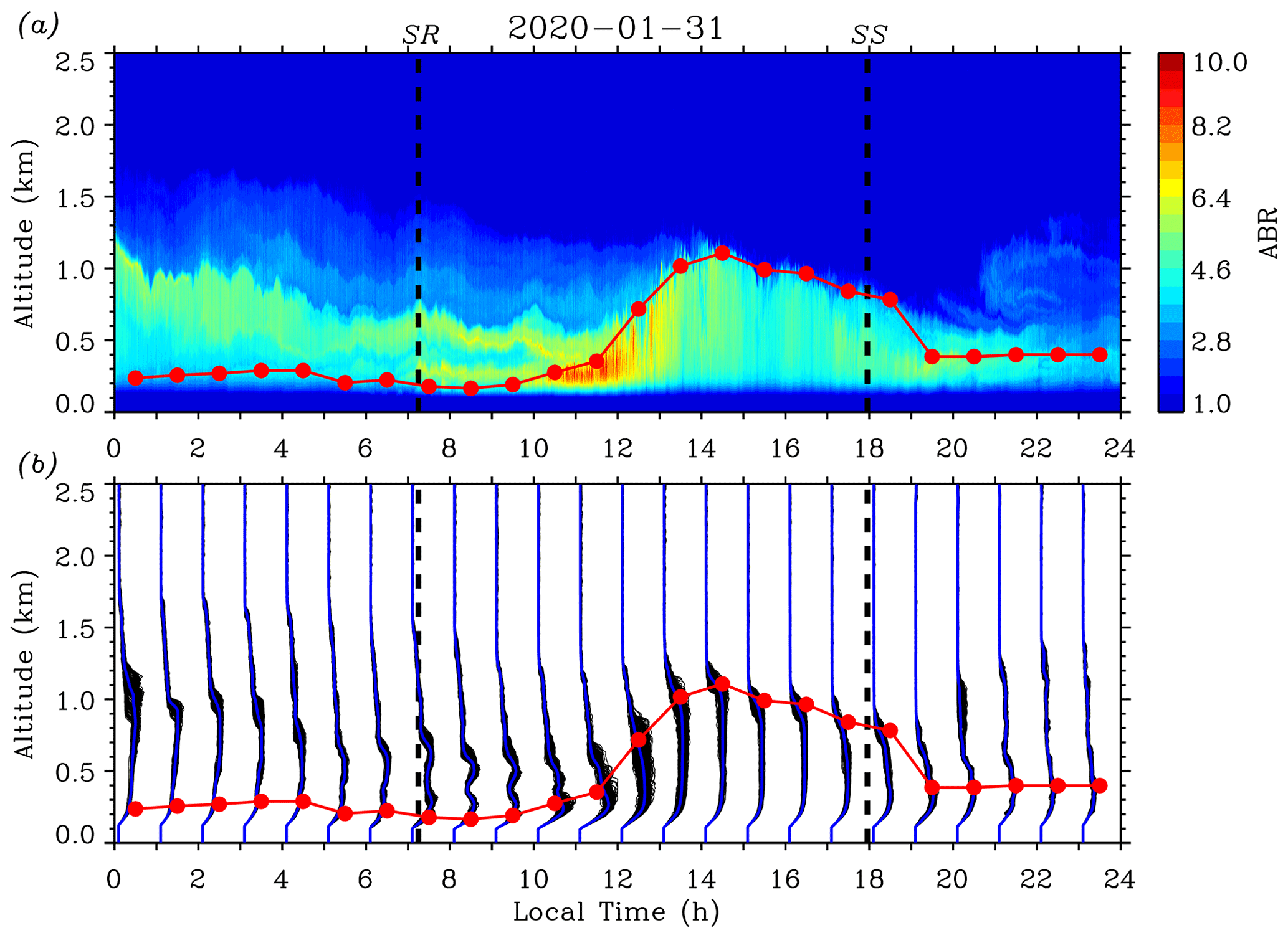
Figure 4 (a) Contour plot of the ABR on 31 January 2020. (b) Over-plots of ABR profiles (thin black lines) in each 1 h time interval and the hourly mean ABR profile (blue lines). SR and SS times are indicated by thick black dashed lines. Red solid circles represent the hourly mean ABL depth retrieved by using the variance method and the red line indicates the diurnal evolution trend of the ABL depth.

4.1 Case study 1 (31 January 2020)

Figure 4 presents a full-day measurement result of the ABL performed in late winter. Figure 4a provides a time–height contour plot (10 s time and 6.5 m height resolution) of the ABR on 31 January 2020. It is seen that the atmosphere was quite clear in height ranges between 1.7 and 2.5 km, while multiple (residual) aerosol layers were present below 1.7 km until 14:00 LT when they were totally “engulfed” by the well-developed CBL. Advected aerosol layers above ∼ 0.6 km were also discernible after 19:30 LT. In spite of the presence of these aerosol layers aloft, the variance method is first applied to retrieve the hourly mean ABL depth for each 1 h time interval. Before finding a local maximum from the calculated ABR-variance profile, the proper upper and lower height limits are determined by visualizing the corresponding D(z) and W_f(z) contour plots (see Fig. 2). Then, the height with local maximum variance between the chosen upper and lower heights is searched for and located as the ABL depth (red solid circles). SR and SS times are indicated by thick black dashed lines. As shown by Fig. 4a, the values of the ABR in the CBL had a direct “response” to the development of CBL depth: between ∼ 10:30 and 11:30 LT when the initial CBL was shallow (CBL depth < 0.35 km), the ABR had larger values reaching 10; then, as the CBL depth increased and reached to a maximum of ∼ 1.02 km around 13:30 LT, the ABR values in the CBL generally decreased. If we assume that in the lidar observation time interval the probed aerosols did not undergo chemical and physical reactions, then the change in ABR values can be regarded as the change of aerosol number density in the CBL (Engelmann et al., 2008; Pal et al., 2010). Figure 4a graphically describes the vertical transport of aerosols from the surface to upper heights. As the available dispersion volume (CBL depth) enlarges, the ABR values (the mixed aerosol number density) fall. Between 13:30 and 18:30 LT, the ABR values in the CBL exhibited features of vertical homogeneity (see Fig. 4b), indicating the full mixing of aerosols in the ML.

Figure 4b over-plots the ABR profiles (thin black lines) in each 1 h time interval. The hourly mean ABR profile is also added (blue lines). It is found that the fluctuation features of the over-plotted ABR profiles differ at distinct developing stages of the CBL. In the time interval between ∼ 08:30 and 11:30 LT, the hourly mean CBL depth grew slowly from ∼ 0.18 km at around 08:30 LT to ∼ 0.35 km at around 11:30 LT; meanwhile, fluctuations of the over-plotted ABR profiles increased in this initial CBL. This stage corresponds to the formation period of the CBL (Stull, 1988). After SR, the sun started to heat the surface. Consequently, convective activities started to occur and CBL began to develop, but the CBL depth growth was restricted by the upper stable NBL (Stull, 1988). Then, the hourly mean CBL depth increased rapidly from ∼ 0.35 km at around 11:30 LT to ∼ 1.02 km at around 13:30 LT. Fluctuations of the over-plotted ABR profiles kept increasing throughout the CBL at first then decreased and tended to become uniform in the middle and lower parts of the CBL. This stage denotes the rapid growth period of the CBL (Stull, 1988). After ∼ 11:30 LT the cool NBL air was warmed to a temperature near that of the above RL and the CBL top had reached the base of the RL. At this point, the stable NBL capping the CBL vanished, so that thermals could penetrate upward quickly, allowing the growth of the CBL depth with a larger growth rate. However, this rapid growth did not continue after the CBL depth reached the top of the RL, where the FA above prevented thermals from further vertical motion (Stull, 1988). Accompanying the initial penetrating thermals upward, aerosols (as well as other constituents) were transported vertically and turbulently mixed, exhibiting a high fluctuation feature for the ABR in the CBL. While vertical transport and turbulent mixing continued, aerosols were fully mixed in a larger available volume, reflected by both smaller fluctuations of the ABR profiles and the values of the ABR themselves. Next, the hourly mean CBL depth changed very little from ∼ 1.02 km at around 13:30 LT to ∼ 0.96 km at around 16:30 LT; fluctuations of the over-plotted ABR profiles kept decreasing until all the ABR profiles became uniformly upright below the top area of the CBL. This stage represents the quasi-stationary period of the CBL (Stull, 1988). The little change of the CBL depth is governed by the balance between entrainment and subsidence (Stull, 1988). In this stage, the aerosols had been fully and evenly mixed in the ML, indicated by the smallest fluctuations of the ABR profiles and values of the ABR. Finally, in the late afternoon, the hourly mean ABL depth kept decreasing from ∼ 0.96 km at around 16:30 LT to ∼ 0.39 km at around 19:30 LT; fluctuations of the over-plotted ABR profiles increased slightly in the ML. This stage describes the decay period of the CBL (Stull, 1988). As the solar radiation weakened, the strength of convective turbulence reduced so that turbulence could not be maintained against dissipation (Nieuwstadt et al., 1986). The small increase in ABR fluctuations reflected that the decay turbulence could no longer preserve the homogeneous distributions of the aerosols in the ML. After SS, the turbulence in the ML might decay completely; then the layer needed to be re-categorized as an RL while at the same time the NBL had already formed near surface. It should be noted that for all four stages, obvious fluctuations of the over-plotted ABR profiles were always present near the top area of the CBL. This fluctuating behavior looked like a “node”, representing the structure of the EZ between the CBL and FA (Kong and Yi, 2015).

Figure 5 further investigates the evolution of the CBL depth on 31 January 2020. Figure 5a plots the instantaneous CBL depths (blue) obtained by using the LGM method (before 10:00 and after 19:00 LT) and HWT method (between 10:00 and 19:00 LT). For comparison, the hourly mean ABL depths (red solid circles) from the variance method are added. Figure 5b shows the corresponding hourly mean ABL depth growth rate. At the formation stage, the CBL depth growth rate changed sign from negative to positive at ∼ 08:30 LT and reached a maximum of ∼ 0.084 km/h at around 10:00 LT. After SR, the ABL depth did not increase immediately, but some time later (the growth rate be negative before ∼ 08:30 LT). The time interval between SR and 11:30 LT is roughly defined as the early morning transition (EMT) period (Pal et al., 2010). During this EMT period, the instantaneous CBL depth generally exhibited a small deviation from that indicated by the hourly mean ABL depth (red line). At the growth stage, the CBL depth increased with a mean growth rate of > 0.3 km/h and a maximum growth rate of ∼ 0.36 km/h at around 12:00 LT. Meanwhile, the instantaneous CBL depths showed obvious larger deviations and fluctuations. At the quasi-stationary stage, the CBL depth growth rate changed sign at around 14:30 LT and varied between 0.09 and −0.12 km/h. The accompanying instantaneous CBL depths had comparatively moderate deviations and fluctuations. At the final decay stage, the ABL depth growth rate stayed negative with a minimum of −0.40 km/h at around 19:00 LT. The fluctuations of instantaneous CBL depth were generally moderate before SS. The ABL depth growth rate returned to nearly zero at ∼ 20:00 LT and the time interval between SS and 20:00 LT is roughly defined as the early evening transition (EET) period (Pal et al., 2010). During this EET period, the instantaneous ABL depth exhibited a small deviation from that indicated by the hourly mean ABL depth (red line).

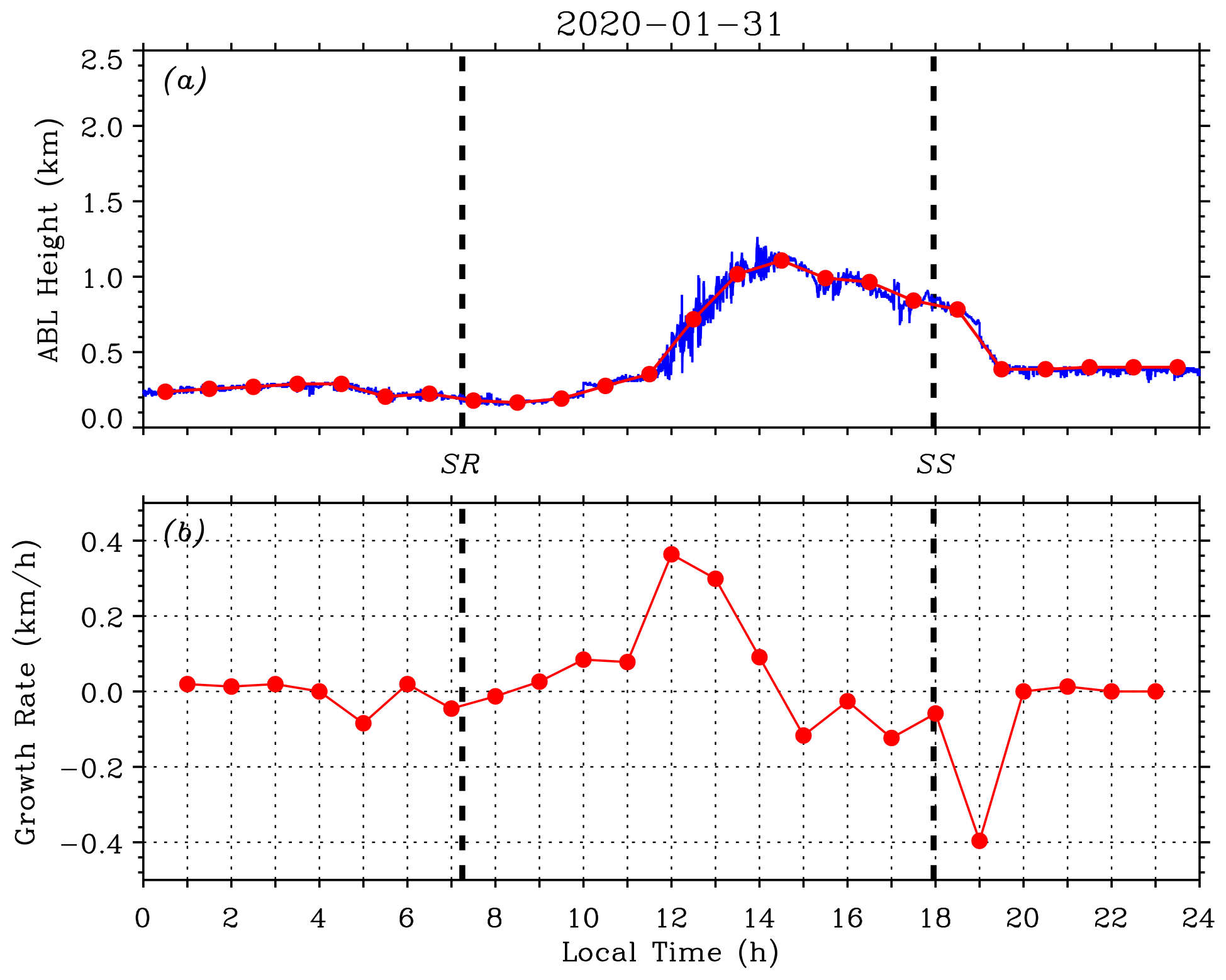
Figure 5 (a) Instantaneous ABL depths (blue) obtained using the LGM method (before 10:00 and after 19:00 LT) and HWT method (between 10:00 and 19:00 LT). Red solid circles indicate the hourly mean ABL depth from the variance method. (b) Hourly mean ABL depth growth rate. Thick black dashed lines mark the SR and SS times on 31 January 2020.

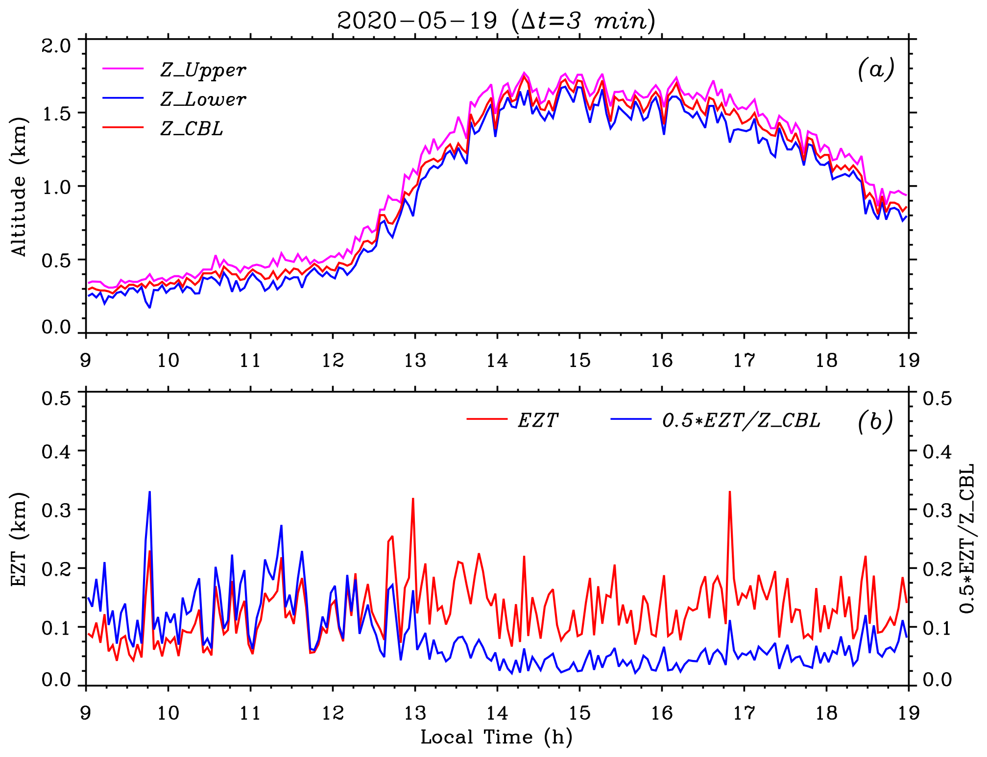
It is visually observable that the time series of instantaneous CBL depths fluctuate on small timescales (Fig. 5a), especially in the growth stage, reflecting the entrainment characteristics in the EZ. To some extent, the EZT can serve as a measure of averaged vertical size of the ABL depth fluctuation (Boers et al., 1995). Hence, the EZT is calculated and investigated here. Figure 6a plots the CBL depth Z_CBL (red) obtained by using the variance method between 09:00 and 19:00 LT on 31 January 2020. The EZ upper height Z_Upper (magenta) and lower height Z_Lower (blue) are determined from the FWHM of the σ(ABR) profile (see Fig. 3). To generate one σ(ABR) profile, a group of 18 consecutive ABR profiles in a time interval of 3 min is utilized so that the retrieved Z_CBL and EZT represent the corresponding mean values in each given time interval of 3 min. Here, the choice of 3 min is a compromise between the time resolution of the EZT and the reliability of σ(ABR) profile. Figure 6b exhibits the resulting EZT (red) and ratio of EZT to Z_CBL (blue; for convenience, the ratio is multiplied by a factor of 0.5 so that the two vertical axes share the same scaling range). The overall EZT time series between 09:00 and 19:00 LT had a minimum (min) of 26 m, a maximum (max) of 267 m and a mean (mean) of 94 m with a standard deviation (SD) of 38 m. The ratio values spanned a range from 3.5 % to 76.8 %. Larger ratio values (> 30 %) mainly appeared in the formation stage and first half of the growth stage of the CBL (before 12:30 LT), while most ratio values were < 20 % after the second half of the growth stage (after 12:30 LT).

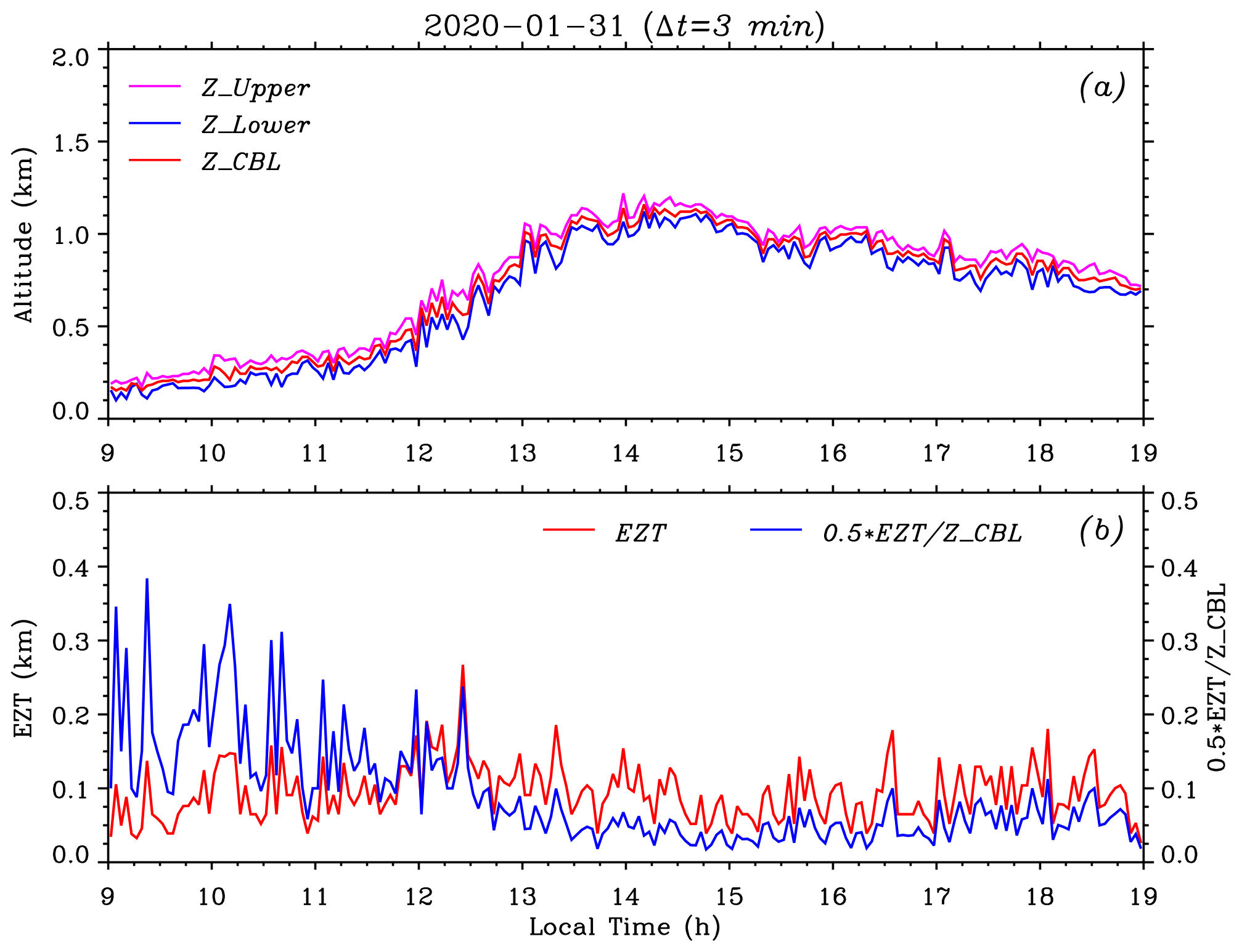
Figure 6 (a) The CBL depth Z_CBL (red) obtained using the variance method between 09:00 and 19:00 LT on 31 January 2020. The EZ upper height Z_Upper (magenta) and lower height Z_Lower (blue) are derived from the FWHM of the σ(ABR) profile, each of which is calculated within a time interval of 3 min. (b) The corresponding EZT (red) and ratio of EZT to Z_CBL (blue) during the same time interval. Note that the ratio is multiplied by a factor of 0.5 so that the two vertical axes share the same scaling range.

Table 1 Statistics of the EZT obtained on 31 January 2020.

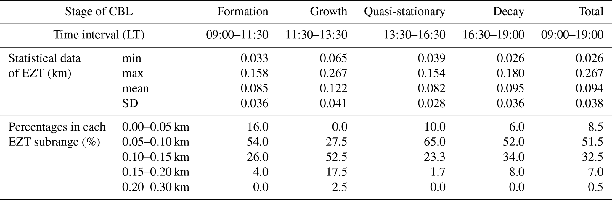
Table 1 summarizes the corresponding statistical data for all four developing stages of the CBL on 31 January 2020. It is seen that the growth stage had the largest EZT statistical data (a min of 65 m, a max of 267 m, a mean of 122 m and an SD of 41 m). On the contrary, the quasi-stationary stage exhibited lower EZT statistical data (a max of 154 m, a mean of 82 m and an SD of 28 m, except for a min of 39 m). The formation stage (a min of 33 m, a max of 158 m, a mean of 85 m and an SD of 36 m) and decay stage (a min of 26 m, a max of 180 m, a mean of 95 m and an SD of 36 m) showed comparable statistics of the EZT. Generally, the overall mean of the EZT varied moderately from stage to stage between 82 and 122 m. When the values of EZT are divided into five subranges (see Table 1 for details), it is observed that the formation stage had the highest percentage of 16.0 % of the EZT falling into the 0–50 m subrange, while the growth stage had none falling into the same subrange. However, the growth stage had the largest percentage of 17.5 % of the EZT falling into the 150–200 m subrange, and was the unique stage having EZT values exceeding 200 m. The quasi-stationary stage had the smallest percentage of 1.7 % of the EZT falling into the 150–200 m subrange. For all four stages, the EZT values mostly fell into the 50–100 m and 100–150 m subranges with corresponding cumulative percentages of 80.0 %, 80.0 %, 88.3 % and 86.0 %, respectively.

Figure 7 Same as Fig. 4 but on 19 May 2020.

4.2 Case study 2 (19 May 2020)

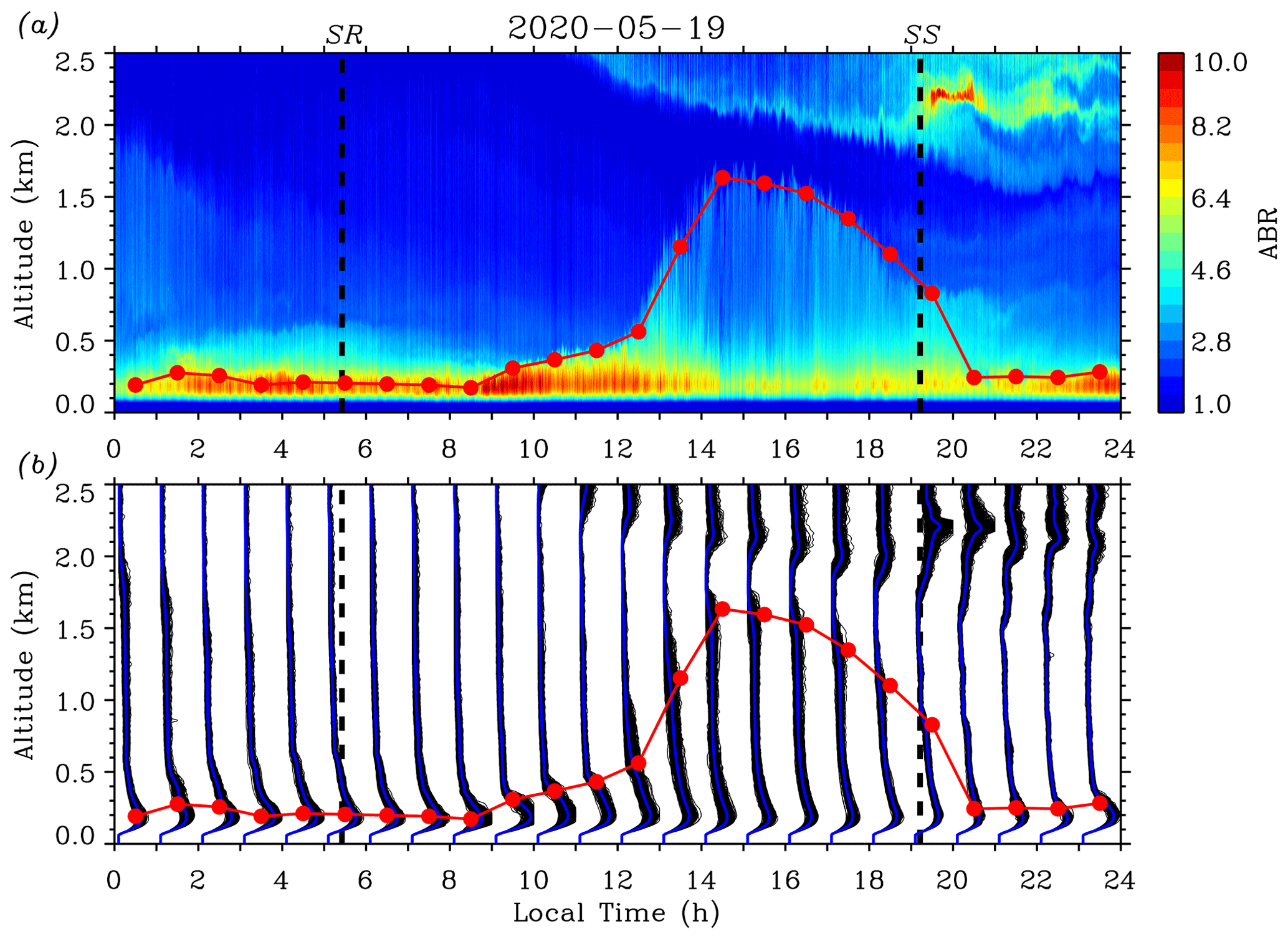
Figure 7 presents a full-day measurement result of the ABL executed in late spring. Figure 7a provides the time–height contour plot (10 s and 6.5 m resolution) of the ABR on 19 May 2020. On this late spring day, there were less abundant aerosols above 0.6 km compared to below 0.6 km between 00:00 and 12:00 LT. Another advected aerosol layer starting at around 09:00 LT (not indicated here) above 1.5 km subsided but did not interfere with the lower ABL. The variance method is first used to determine the hourly mean ABL depth for each 1 h time interval (red solid circle). The ABR before 10:30 LT showed large values (> 8) in the initial CBL below 0.4 km. Then, as the CBL depth (red line) increased and reached a maximum of ∼ 1.63 km at around 14:30 LT, the ABR values in the CBL exhibited a decrease below 0.4 km and a general increase between 0.4 km and 1.0 km, indicating the turbulent transport of aerosols from surface to upper heights. Figure 7b over-plots the ABR profiles (thin black lines) in each 1 h time interval and the hourly mean ABR profile (blue line). In the formation period of the CBL, the hourly mean CBL depth grew slowly from ∼ 0.18 km at around 08:30 LT to ∼ 0.56 km at around 12:30 LT; fluctuations of the over-plotted ABR profiles prevailed throughout the CBL. Then, in the growth period of the CBL, the hourly mean CBL depth increased rapidly from ∼ 0.56 km at around 12:30 LT to ∼ 1.63 km at around 14:30 LT; observable fluctuations of the over-plotted ABR profiles continued, but tended to decrease and become uniform in the middle part of the CBL. Next, in the quasi-stationary period of the CBL, the hourly mean CBL depth changed very little from ∼ 1.63 km at around 14:30 LT to ∼ 1.52 km at around 16:30 LT; fluctuations of the over-plotted ABR profiles decreased slightly and all the ABR profiles became uniformly upright in the middle part of the CBL. Finally in the decay period of the CBL, the hourly mean ABL depth kept decreasing from ∼ 1.52 km at around 16:30 LT to ∼ 0.24 km at around 20:30 LT; both fluctuations of the over-plotted ABR profiles and ABR values exhibited a small decrease in the middle and lower part of the CBL. Again, for all four periods, obvious fluctuations of the over-plotted ABR profiles were always present near the top area of the CBL.

Figure 8 Same as Fig. 5 but on 19 May 2020.

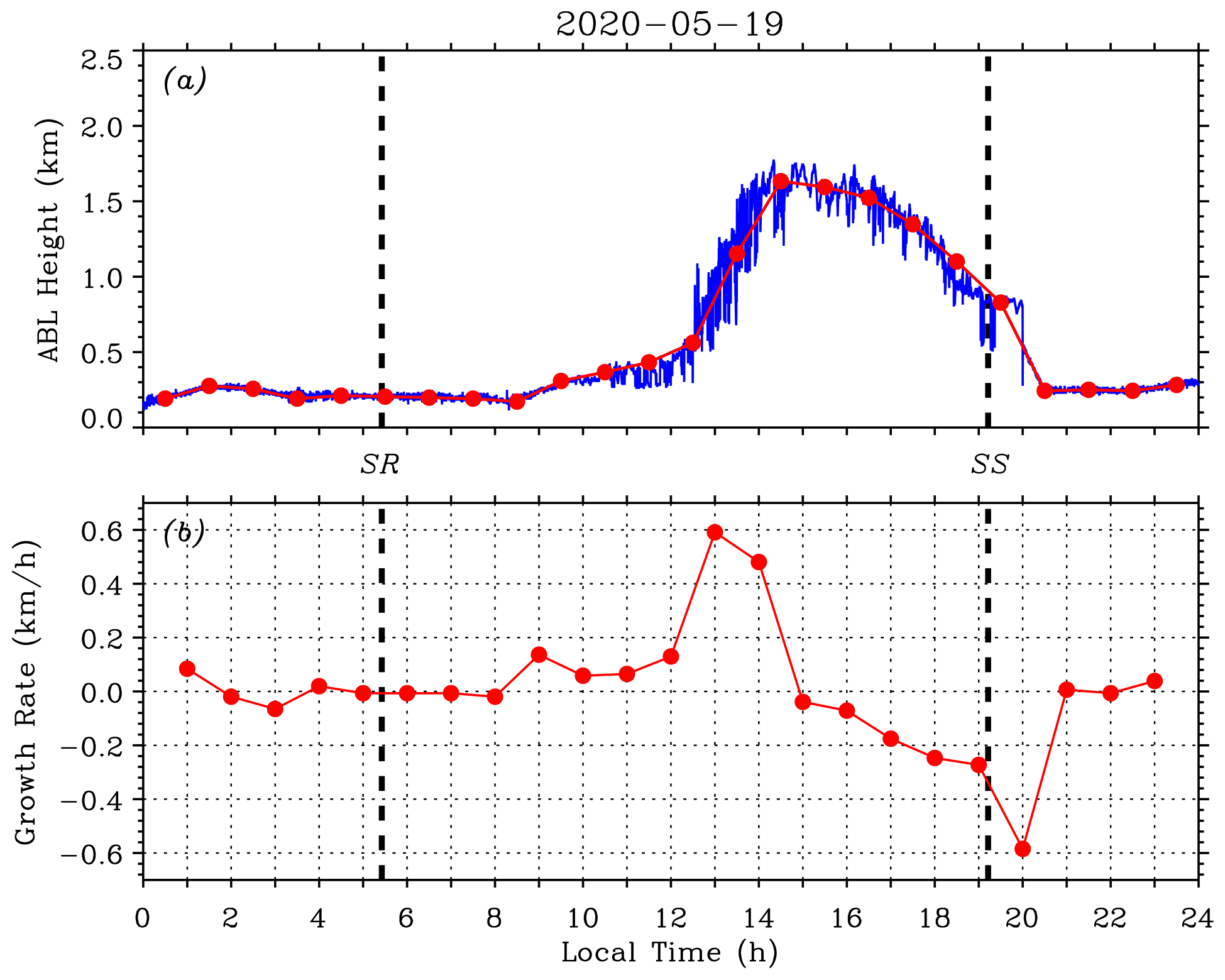
Figure 8a plots the instantaneous CBL depth (blue) obtained using the LGM method (before 09:00 and after 20:00 LT) and HWT method (between 09:00 and 20:00 LT). The hourly mean ABL depths (red solid circles) from variance method are added. Figure 8b shows the hourly mean ABL depth growth rate (red solid circles). At the formation stage, the CBL depth growth rate changed sign from negative to positive at ∼ 08:00 LT and reached a maximum of ∼ 0.14 km/h at around 09:00 LT. The EMT period is roughly defined between SR and 12:00 LT. The instantaneous CBL depths exhibited a small deviation from that indicated by the hourly mean ABL depth (red line) before 10:00 LT but showed increased deviation later on. At the growth stage, the CBL depth increased with a mean growth rate of > 0.48 km/h and a maximum growth rate of ∼ 0.59 km/h at around 13:00 LT; meanwhile, the deviations and fluctuations of the instantaneous CBL depths obviously enlarged. At the quasi-stationary stage, the CBL depth growth rate changed sign to negative at around 15:00 LT and varied between −0.04 and −0.07 km/h; the fluctuations of the instantaneous CBL depth remained obvious. At the final decay stage, the ABL depth growth rate kept negative with a minimum of −0.58 km/h at around 20:00 LT; the fluctuations of instantaneous ABL depth were still observable. The ABL depth growth rate returned to nearly zero at ∼ 21:00 LT and the time interval between SS and 21:00 LT is roughly defined as the EET period. During the EET period, the instantaneous ABL depth generally exhibited a small deviation from that indicated by the hourly mean ABL depth (red line). Note that after SS, the CBL should be re-categorized as an RL.

Figure 9a plots the CBL depth Z_CBL (red) obtained using the variance method between 09:00 and 19:00 LT on 19 May 2020 as well as the EZ upper height Z_Upper (magenta) and lower height Z_Lower (blue) derived from the FWHM of the σ(ABR) profile. Figure 9b shows the resulting EZT (red) and ratio of EZT to Z_CBL (blue). The overall EZT time series between 09:00 and 19:00 LT had a min of 42 m, a max of 331 m and a mean of 127 m with an SD of 49 m. The ratio values varied between 4.2 % and 66.2 %. Larger ratio values (> 30 %) mainly occurred in the formation stage and the initial of growth stage of the CBL (before 13:15 LT), while most ratio values were < 20 % later on (after 13:15 LT).

Table 2 Statistics of the EZT obtained on 19 May 2020.

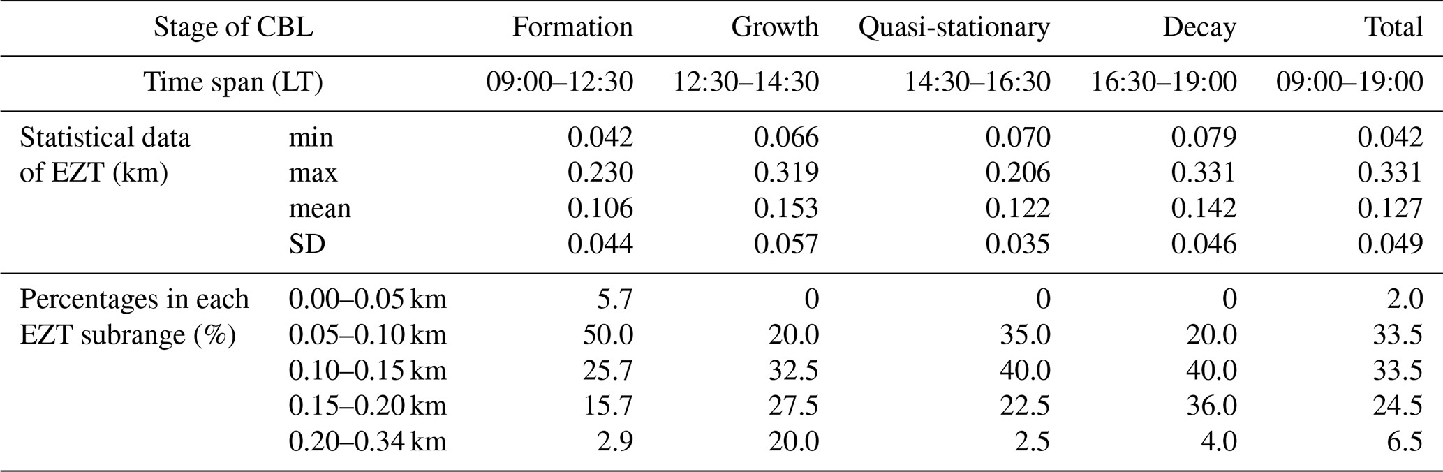
Table 2 summarizes the corresponding statistics for all four developing stages of the CBL on 19 May 2020. It can be seen that the growth stage had the largest mean (153 m) of the EZT, while the formation stage exhibited the lowest mean (106 m) of the EZT. Furthermore, the growth stage and quasi-stationary stage had the largest SD (57 m) and the smallest SD (35 m) of the EZT, respectively. The overall mean of the EZT varied moderately from stage to stage between 106 and 153 m. When the values of the EZT are divided into five subranges (see Table 2 for details), it is found that the formation stage had a percentage of 5.7 % of the EZT falling into the 0–50 m subrange, while the other three stages had none falling into the same subrange. For this late spring case, all four stages had percentages of > 15 % of the EZT falling into the 150–200 m subrange, and the growth stage exhibited the largest percentage of 20.0 % of the EZT exceeding 200 m. For all four stages, the EZT had values mostly falling into the range between 50 and 150 m with corresponding percentages of 75.7 %, 52.5 %, 75 % and 60.0 %, respectively.

Figure 9 Same as Fig. 6 but on 19 May 2020.

4.3 Discussion of the clear-day EZT statistics and the FWHM method

In combination with the two typical cases presented above, another two clear-day cases (on 7 September and 12 November 2020) are also investigated to demonstrate the robustness of the FWHM method and the representativeness of the conclusions on the EZ. The corresponding contour plots of the ABR, plots of the ABL depth and EZT evolution as well as tables of obtained EZT statistics are provided in the Supplement. Since no suitable clear-day case is available for the summer days of 2020 due to rainy and/or patchy-cloudy weather conditions, the early autumn result on 7 September 2020 is selected here and regarded as representative of a summer case as the surface temperatures on this day (21–34 ^∘C) were comparable with those on summer days (20–37 ^∘C; see Table S3 in the Supplement). Table 3 compares the EZT statistics for all four cases.

Table 3 Comparison of the EZT statistics for the four typical cases.

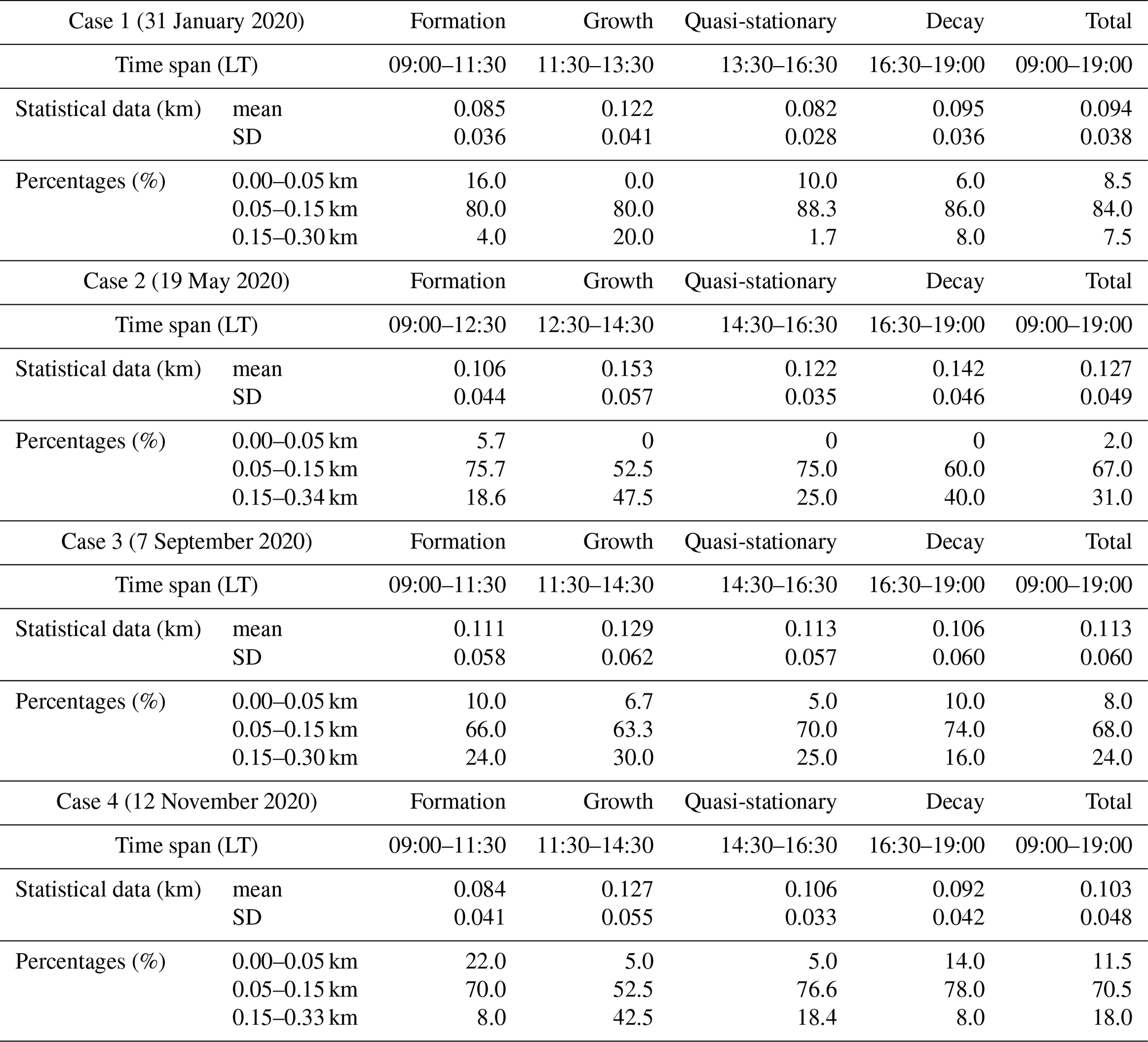
As shown in Table 3, all four cases exhibited apparent statistical differences. For the same time interval of 09:00–19:00 LT, the winter case (case 1; a mean of 94 m, an SD of 38 m) and the late autumn case (case 4; a mean of 103 m, an SD of 48 m) had overall statistical EZT data smaller than those of the late spring case (case 2; a mean of 127 m, an SD of 49 m) and the early autumn case (case 3; a mean of 113 m, an SD of 60 m). Note that this statistical conclusion was also true for each of the four developing stages. In addition, the winter case (8.5 %) and the late autumn case (11.5 %) had larger percentages of the EZT falling into the subranges of 0–50 m than those of the late spring case (2.0 %) and the summer case (8.0 %), but smaller percentages (7.5 % and 18.0 %, respectively) of the EZT falling into the subranges of > 150 m compared to those of the late spring case (31.0 %) and the summer case (24.0 %). The reason for larger EZT statistics (mean and SD) and higher percentage (possibility) of larger EZT values (> 150 m) for the late spring and early autumn cases is attributed to the stronger solar radiation reaching the earth's surface in late spring/early autumn than in winter/late autumn (Guo et al., 2020). Stronger solar radiation generally results in more vigorous and frequent thermals overshooting to higher heights (updrafts) and then moving back (downdrafts). Consequently, entrainments take place in larger vertical regions. Hence, both the EZT statistics (mean and SD) and the possibility of larger EZT values seem to provide measures of entrainment intensity. There were also common characteristics for the four observational cases. For example, all four cases showed moderate variations of the mean of the EZT from stage to stage. The growth stage always had the largest mean and SD of the EZT; as neither the NBL nor the FA restricts the booming development of the CBL in the growth stage, the entrainments were allowed to occur in a wider vertical range. In addition, the quasi-stationary stage usually had the smallest SD of the EZT; this quantitatively reflected the fact that the CBL depth and the EZT changed little in this stage. For all four stages, most EZT values fell into the 50–150 m subrange; the corresponding overall percentages of the EZT falling into the 50–150 m subrange between 09:00 and 19:00 LT were 84 %, 67 %, 68 % and 70.5 % for the winter, late spring, early autumn and late autumn cases, respectively.

Note that the proposed FWHM method utilizes the FWHM of the variance profile of the ABR fluctuations to quantify the EZT. We believe it to be physically sound as it directly reflects the mixing history of aerosols (tracers) in the EZ. When applying it to lidar data, it definitely determines the EZ (and consequently the EZT) when turbulence is dominating and the variance profile of ABR fluctuations has clear-cut edges. However, caution must be taken when turbulence is weak and the variance profile of the ABR fluctuations suffers from interference of residual layer and/or advected aerosols. The retrieved EZT values for the four typical clear-day cases mostly fall into the 50–150 m range with a percentage of ≥ 67 %, while the overall EZT values range from 0 to 340 m. Pal et al. (2010) reported the lidar-derived EZT retrievals for a summer case using the cumulative frequency distribution method, which had mean values of 75 m and 62 m and magnitude ranges of 10–230 and 0–200 m for the quasi-stationary and growth stages, respectively. For the early autumn case in this work, the EZT results had mean values of 113 and 123 m and magnitude ranges of 41–279 and 39–289 m for the quasi-stationary and growth stages, respectively. These observational results obviously differ for the mean EZT values and magnitude ranges, but this comparison does not seem rigorous as the EZT results were obtained at distinct observational locations. For a better validation of the reliability of the FWHM approach, comparisons with EZT values retrieved by co-located intensive radiosonde or by the synergy of high-resolution temperature lidar (Behrendt et al., 2015) and Doppler lidar (Ansmann et al., 2010), in which case the EZT might be determined by its theoretical definition that corresponds to the vertical region with mean negative buoyancy flux (Driedonks and Tenneke, 1984; Cohn and Angevine, 2000), shall be favored in the future.

5 Summary and conclusions

Continuous and high-resolution measurements of both the convective boundary layer (CBL) and associated entrainment zone (EZ) are of significant importance to boundary layer studies, including land–atmosphere interactions, air quality forecasts and almost all weather and climate models. This work presents the high-resolution measurement results of the CBL and associated EZ using a recently developed titled polarization lidar (TPL) over Wuhan (30.5^∘ N, 114.4^∘ E). The TPL is housed in a customized working container and capable of operating under various weather conditions. The TPL has an inclined working angle of 30^∘ off zenith and routinely monitors the atmosphere with a time resolution of 10 s and a height resolution of 6.5 m. The equivalent minimum height with full overlap for the TPL is ∼ 173 m a.g.l. (above ground level).

From the lidar-recorded range-square corrected elastic signal X, the two vertical-distribution-based methods (logarithm gradient method (LGM) and Harr wavelet transform method (HWT)) are tested to retrieve instantaneous ABL depths for each X profile. Before applying the LGM and HWT methods, the process-based variance method is first used to locate the hourly mean ABL depth. For each given 1 h time interval, the height with maximum variance in the variance profile of aerosol backscatter ratio (ABR) fluctuations is searched for as the hourly mean ABL depth. By visualizing the time–height contour plots of D(z) (defined as derivative of logarithmic X) and W_f(z) (defined as covariance transform value of X), the proper upper height limits needed for choosing the true height with local maximum variance are intuitive and convenient to be correctly determined as the base of the misleading aerosol layers aloft. Then, the hourly mean ABL depths provide a guide for an automated attribution of instantaneous ABL depth by using the LGM and HWT methods. A new approach utilizing the FWHM of the variance profile of ABR fluctuations is developed and proposed to determine the entrainment zone thickness (EZT). This approach is believed to be physically sound as it directly reflects the mixing history of aerosols (tracers) in the entrainment zone (EZ).

Two out of four cases of the TPL clear-day measurement results of the CBL and associated EZ are presented. It is concluded that the CBL depth evolution can be described by four consecutive stages. At the formation stage, the hourly mean CBL depth grew slowly with a smaller positive growth rate. At the growth stage, the hourly mean CBL depth grew fast with a larger positive growth rate. At the quasi-stationary stage, the hourly mean CBL depth varied slightly and the hourly mean CBL depth growth rate changed sign from positive to negative. At the decay stage, the hourly mean CBL depth kept decreasing until the layer was re-categorized as a residual layer.

The instantaneous CBL depths exhibited different fluctuation magnitudes in the four stages and the growth stage always had larger fluctuations. The fluctuations of over-plotted ABR profiles in each 1 h time interval also showed different behaviors at respective stages; the fluctuations usually enlarged at the formation stage, while generally decreased in the middle part of the CBL at the late growth and quasi-stationary stages. However, the fluctuations of over-plotted ABR profiles always prevailed near the top area of the CBL, reflecting the structures of the EZ.

The EZT is subsequently investigated in detail using the proposed FWHM method. It is found that for the same statistical time interval of 09:00–19:00 LT, the four cases differ in mean (mean) and standard deviation (SD) of EZT data as well as percentages of EZT values falling into distinct subranges. In detail, the winter case (a mean of 94 m, an SD of 38 m) and the late autumn case (a mean of 103 m, an SD of 48 m) had overall statistical EZT data smaller than those of the late spring case (a mean of 127 m, an SD of 49 m) and the early autumn case (a mean of 113 m, an SD of 60 m). Moreover, this statistical conclusion was also true for each of the four developing stages. In addition, the winter case (8.5 %) and the late autumn case (11.5 %) had larger percentages of the EZT falling into the subranges of 0–50 m than those of the late spring case (2.0 %) and the early autumn case (8.0 %), but smaller percentages (7.5 % and 18.0 %, respectively) of the EZT falling into the subranges of > 150 m compared to those of the late spring case (31.0 %) and the early autumn case (24.0 %). The reason for larger statistical EZT data (mean and SD) and a higher percentage (possibility) of larger EZT values (> 150 m) is attributed to the stronger solar radiation reaching the earth's surface. It seems that both the EZT statistics (mean and SD) and possibility of larger EZT values provide measures of entrainment intensity. Common statistical characteristics also existed. All four cases showed moderate variations of the mean of the EZT from stage to stage. The growth stage always had the largest mean and SD of the EZT and the quasi-stationary stage usually had the smallest SD of the EZT. For all four stages, most EZT values fell into the 50–150 m subrange. The corresponding overall percentages of the EZT falling into the 50–150 m subrange between 09:00 and 19:00 LT are 84 %, 67 %, 68 % and 70.5 % for the winter, late spring, early autumn and late autumn cases, respectively.

We believe that the current lidar-derived characteristics of the CBL and associated EZ can contribute to improving the understanding of the structures and variations of the ABL as well as providing quantitatively observational basis for parameterization of the EZ in numerical models. However, it should be stated that the obtained characteristics of the four-stage evolution of the CBL and the common statistics of the associated EZ hold true for clear-day observations. Actually, it can be much more complicated when heavy aerosol loads and clouds are present. Further investigations on the CBL and associated EZ under various weather conditions shall be presented in our following works.