Deposition of light-absorbing particles in glacier snow of the Sunderdhunga Valley, the southern forefront of the central Himalayas

Anthropogenic activities on the Indo-Gangetic Plain emit vast amounts of light-absorbing particles (LAPs) into the atmosphere, modifying the atmospheric radiation state. With transport to the nearby Himalayas and deposition to its surfaces the particles contribute to glacier melt and snowmelt via darkening of the highly reflective snow. The central Himalayas have been identified as a region where LAPs are especially pronounced in glacier snow but still remain a region where measurements of LAPs in the snow are scarce. Here we study the deposition of LAPs in five snow pits sampled in 2016 (and one from 2015) within 1 km from each other from two glaciers in the Sunderdhunga Valley, in the state of Uttarakhand, India, in the central Himalayas. The snow pits display a distinct enriched LAP layer interleaved by younger snow above and older snow below. The LAPs exhibit a distinct vertical distribution in these different snow layers. For the analyzed elemental carbon (EC), the younger snow layers in the different pits show similarities, which can be characterized by a deposition constant of about 50 µg m⁻² mm⁻¹ snow water equivalent (SWE), while the old-snow layers also indicate similar values, described by a deposition constant of roughly 150 µg m⁻² mm⁻¹ SWE. The enriched LAP layer, contrarily, displays no similar trends between the pits. Instead, it is characterized by very high amounts of LAPs and differ in orders of magnitude for concentration between the pits. The enriched LAP layer is likely a result of strong melting that took place during the summers of 2015 and 2016, as well as possible lateral transport of LAPs. The mineral dust fractional absorption is slightly below 50 % for the young- and old-snow layers, whereas it is the dominating light-absorbing constituent in the enriched LAP layer, thus, highlighting the importance of dust in the region. Our results indicate the problems with complex topography in the Himalayas but, nonetheless, can be useful in large-scale assessments of LAPs in Himalayan snow.

1 Introduction

Aerosol particles in the Indo-Gangetic Plain (IGP) are produced in great mass and number. Being especially prominent in the pre-monsoon season, a large fraction of the airborne aerosols are carbonaceous particles, consisting of organic carbon (OC) and black carbon (BC). Originating from the combustion of fossil fuels and biomass, the particles form the atmospheric brown cloud – known to modify the atmospheric radiation state (Lau et al., 2006; Menon et al., 2010; Ramanathan and Carmichael, 2008). Through air mass transport the aerosol can be conveyed and lifted from the IGP to its northern barrier, the mountains of the Himalayas (e.g., Hooda et al., 2018; Kopacz et al., 2011; Raatikainen et al., 2014; Zhang et al., 2015). Covered with vast amounts of snow and ice, the Himalayan cryosphere is affected by the deposition of carbonaceous aerosol onto its surface (e.g., He et al., 2018; Jacobi et al., 2015; Ménégoz et al., 2014; Xu et al., 2009). This is due to the particulates and especially BC effectiveness in reducing the snow albedo (Warren and Wiscombe, 1980), which ultimately leads to accelerated snowmelt (Flanner et al., 2007; Jacobi et al., 2015; Jacobson, 2004; Ming et al., 2012).

In addition to BC and OC, other particles such as mineral dust (MD) and snow microbes (collectively known as light-absorbing particles – LAPs) are also of importance in reducing snow albedo (e.g., Skiles et al., 2018). In Himalayan snow and ice, the LAP content has been shown to vary significantly, both spatially and temporally (e.g., see review by Gertler et al., 2016). Further, an extensive compilation of BC measurements in snow over the Tibetan Plateau is presented in the Supplement of He et al. (2018), with concentrations ranging from 1 to 3600 ppb_w in the region termed as the Himalayas. In addition to long-range transported LAPs, local sources within the Tibetan Plateau have also been documented to be significant in some regions (e.g., Li et al., 2016), creating several different sources of LAPs in the snow. Varying meteorology- and terrain-induced exchange processes (advection and turbulence) in the mountains further complicates the interplay between the atmospheric deposition of LAPs and the snow surfaces.

Recent modeling studies have reported analogous results, indicating certain sub-regions of the Himalayas to be especially vulnerable to LAP deposition. Santra et al. (2019) simulated the BC impact on snow albedo and glacier runoff in the Hindu Kush–Himalayan region. The authors identified a hot-spot zone for BC in the vicinity of Manora Peak, located in the Indian state of Uttarakhand, in the central Himalayas (also sometimes called the western Himalayas depending on classification). The BC induced a greater albedo reduction on glacier snow in the vicinity of this hot-spot area compared to other areas in the Hindu Kush–Himalayan area. Similarly, another modeling study simulated the impact of LAPs on High Mountain Asia snow albedo and its associated forcing and identified the same general area as a region where snow is especially affected by LAP-caused snow darkening (Sarangi et al., 2019). Both of these studies (as well as the work of He et al., 2018) emphasized the need for more in situ measurements of LAPs in the snow of this region of the Himalayas.

Previously, we reported in Svensson et al. (2018) the measured LAP concentrations and properties in the snow from two glaciers in the Sunderdhunga Valley, located in Uttarakhand, India, in the central Himalayas. While we mainly focused on the surface snow layer and characterizing the LAPs, results from one 1.2 m deep snow pit were also presented. Based on the LAP concentration profile and pit stratigraphy, the pit was estimated to represent five seasons. Newly sampled snow pits have since then been analyzed from the same two glaciers, along with available automatic weather station (AWS) data from the same valley. Here we revisit the previous interpretation of the published pit (in Svensson et al., 2018) and report the results of our newly sampled snow pits. By comparing the BC profiles among six pits we aim at quantifying the deposition of elemental carbon (EC; used here as a proxy for BC) in this area of the Himalayas. In addition, we explore the relative contribution of MD to LAPs in the different pits.

2 Methodology

2.1 Glaciers snow sampling and filtration

Snow was collected on the Bhanolti and Durga Kot glaciers during a field campaign in the Sunderdhunga Valley (located in the district of Bageshwar) in October 2016. The two glaciers are positioned adjacent to each other in a general northeast–southwest orientation (cf. Fig. 1) on the southern fringe of the Himalayan mountain range and are further described in Svensson et al. (2018). Local emissions of carbonaceous aerosol in the Sunderdhunga Valley are very limited. The valley is not accessible by car, and the glaciers are at a 3 to 4 d hike from the nearest road. On route to the glaciers the last settlement is Jatoli, located in a river valley at an elevation of 2400 m a.s.l. about 10 km southeast in a perpendicular orientation to the glacier valley. Biomass burning is a common practice for cooking and heating in Jatoli; thus some emissions from the village may enter the glacier valley. It is expected, however, that the majority of carbonaceous particles in the glacier valley originate from regional and long-distance transport. The relatively low elevation span as well as the glaciers' position on the southern slopes of the Himalayas nonetheless make them more prone to LAP deposition compared to other glaciers in the Himalayan Plateau and Tibetan Plateau. Previous studies have reported elevated LAP content in lower elevation snow for Himalayan glaciers (e.g., Ming et al., 2013) and higher concentrations of LAPs in glaciers on the southern edge of the Himalayas (e.g., Xu et al., 2009).

Figure 1 Map of the glaciers with the location of the snow pits (black dots), with the AWS indicated with a star. Dashed lines on the glacier refer to isolines.

On the Durga Kot glacier two snow pits (hereafter pits A and B; Fig. 1) were dug in the vicinity of each other (∼20 m) in an reachable area of the percolation zone of the glacier. The Bhanolti glacier was more easily accessible, and the three excavated snow pits (hereafter pits C–E; Fig. 1) were spread out over a greater distance (∼500 m) on the glacier (see Table 1 and Fig. 1 for additional information). The depth of the pits depended on the level at which a hard layer was found, and digging could not be further conducted with the reinforced shovels with a sharpened edge. The deepest snow pit that was analyzed previously in Svensson et al. (2018), referred to as pit 5 in that study, is from the Bhanolti glacier in September 2015, and we denote it as pit F in the subsequent sections of this paper. As for the other pits from 2016, the depth of pit F was governed by the depth at which the hard layer was encountered.

Table 1 Snow pit details from the Sunderdhunga Valley. Durga Kot glacier snow pits are A and B, while C–F are from the Bhanolti glacier. TC: total carbon.

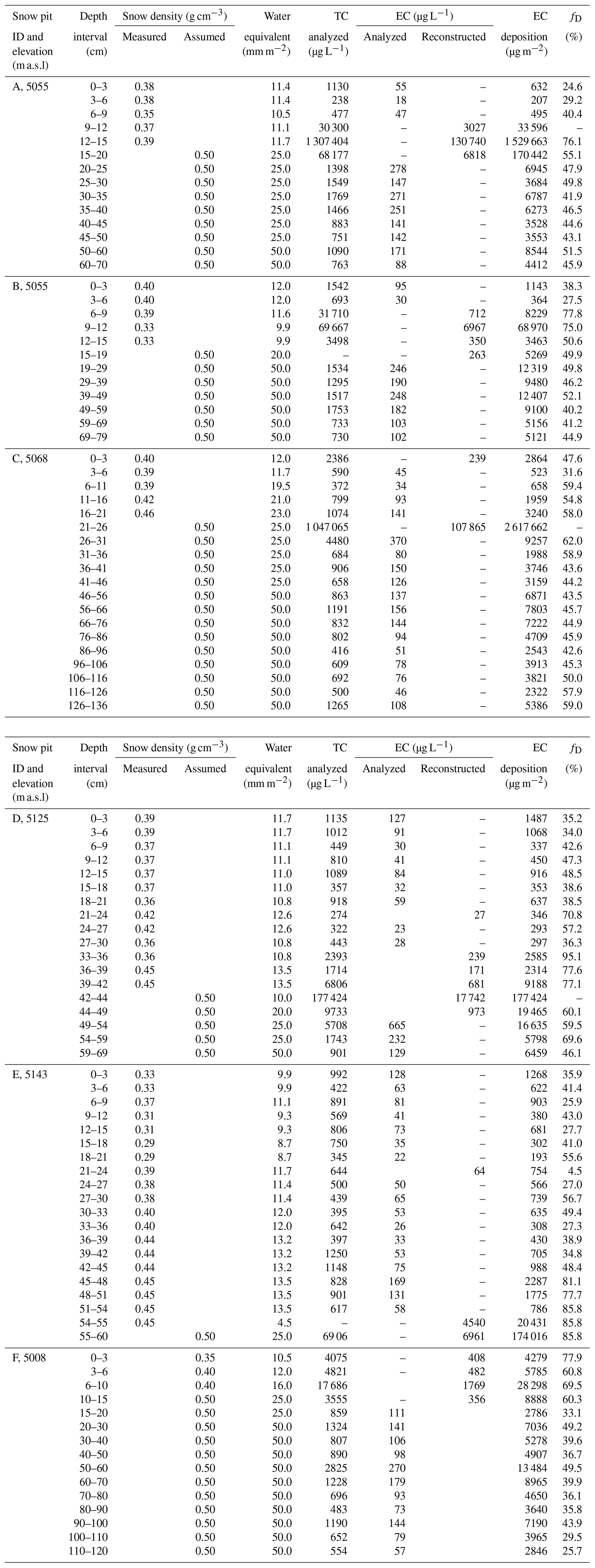
Three distinct, differently colored snow layers could be observed repeating in all but one of the year 2016 pits: a relatively thin (on the order of centimeters), very dark layer was wedged in between white snow above and more grey-appearing snow below (see, e.g., pits B and D in Fig. S1a and b in the Supplement). Due to this stratigraphy, we hereafter simply refer to the whitest snow as young snow, the darkest layer as the enriched LAP layer and the grey snow as old snow. Representative samples ranging from 3 to 10 cm thick layers were taken throughout each pit for analysis of LAPs. Snow density measurements were conducted with a snow density kit in the upper part of the pits (in 5 cm increments) by weighing the known volume of the sampler filled with snow. The observed densities ranged between 0.29 and 0.46 g cm⁻³ (see Table 1 for details). Density measurements were not possible below the enriched LAP layer due to the hard snow. For these layers the density was assumed to be 0.5 g cm⁻³ (to represent aged snow) in our further analyses. Snow density measurements were not conducted for pit F, and we assigned a density of 0.35 g cm⁻³ for the top layer (0–3 cm; similar to observations made in 2016), followed by 0.4 g cm⁻³ between 3 and 10 cm depth and 0.5 g cm⁻³ for all layers below 10 cm. Since the snow samples could not be transported in a solid phase back to the laboratory, they were melted and filtered at the nearby base camp using the same principles as in Svensson et al. (2018). Filters were transported back to the analysis laboratory in petri slides.

2.2 Meteorological observations

In September 2015 an AWS was installed next to the glacier ablation zone of Durga Kot (Fig. 1) about 1.5 km northwards at an elevation below the snow sampling sites. The AWS is equipped with instruments for air temperature, relative humidity (HC2S3-L temperature and relative humidity probe manufactured by ROTRONIC, with a 41303-5A radiation shield), shortwave (SW) and longwave (LW) radiation (upward and downward) (CNR4 four-component net radiometer manufactured by Kipp & Zonen), wind speed and direction (05103-L wind monitor manufactured by R. M. Young, and snow depth (Campbell Scientific  SR50A-L ultrasonic distance sensor). In this paper we use the snow depth data between September 2015 and September 2017 to estimate the local precipitation. The original snow depth data, logged once every 10 min, were filtered to daily resolution by applying a moving median window of 24 h and for the noon value of each day in further analyses. This filtering removed much of the signal noise. However, before this filtering was applied the data were reduced using several logical conditions such as the incoming SW radiation being greater than outgoing SW radiation (to remove errors due to sensors covered by snow) and the surface albedo being greater than 0.2 (to ensure snow cover, as the ground albedo was measured at 0.17). Finally, the consistency between the daily albedo and snow depth was inspected using data presented in Fig. S2a. Each day the snow depth increased was interpreted as precipitation, and to arrive at an estimate of the snow water equivalent (SWE), the fresh-snow density is assumed to be 100 kg m⁻³ (Helfricht et al., 2018). The solid precipitation derived based on the cumulative SWE is presented in Fig. S2b.

2.3 Filter analysis

The analysis of filters followed the procedure in Svensson et al. (2018), with transmission measurements coupled with thermal–optical analysis. According to the measurement nomenclature (Petzold et al., 2013), the carbonaceous constituents measured are EC and OC. The measurement method briefly follows the procedure of placing a filter punch in a custom-built particle soot absorption photometer (PSAP) to measure the transmittance (at λ=526 nm; Krecl et al., 2007) – providing an optical depth for all of the particles captured by the filter. The filter punch is then placed in an OCEC (organic carbon and elemental carbon) analyzer (Sunset instrument, using the EUSAAR_2 protocol; European Supersites for Atmospheric Aerosol Research) to determine the OC and EC mass, followed by another measurement with the PSAP. The OCEC analysis removes the carbonaceous species, and, thus, by comparing the PSAP results obtained before and after the analysis, the relative contribution of the light absorption by EC particles in the total particles optical depth is obtained. The remaining optical depth we attribute as non-EC material. This fraction of the total optical thickness we report as the percentage of the mineral dust absorption on the filter samples (expressed as f_D). For further details concerning the measurements see Svensson et al. (2018).

Some of the filter samples (n=17, out of 91) were saturated with too much light-absorbing material, prohibiting reliable EC measurements despite reducing the sample to a melted equivalent of only 30 mL. To mitigate this problem, we calculated the EC indirectly from the analyzed total carbon (TC) for the saturated samples. From OCEC analysis TC is the most robust measured constituent, since it includes both OC and EC and is not affected by their split point, which may be incorrectly placed for very dark filters (Chow et al., 2001). A slope of 0.099 for the EC / TC ratio for filter samples considered non-saturated was used to reconstruct the EC content for the filter samples containing high amounts of absorbing particles (see details in the Supplement and Fig. S3a and b). The slope compares well with the slopes reported for air samples collected at two sites in the Himalayas about 550 km southeast from Sunderdhunga in the Kathmandu Valley, 32 km (altitude of 2150 m a.s.l.) east of Kathmandu, and Langtang, 60 km north of Kathmandu (altitude of 3920 m a.s.l) (Caricco et al., 2003). There, the authors found that the EC $/$ TC ratio was 0.17 for both sites during the summer monsoon season but between 0.10 and 0.13 during what they described as the ramp-up period and the peak concentration season. The snow samples do not have an upper limit for particles sizes, whereas the air samples were collected as PM_2.5 (particulate matter collected below an aerodynamic diameter of 2.5 µm). The slopes are rather similar to our value, and the authors found as well a very strong correlation of 0.89 (r²) between monthly average EC and OC.

3 Results and discussion

3.1 EC deposition in young- and old-snow samples

When the EC content is analyzed from filtered snow samples, a common practice is to convert the results into mass concentrations [EC], given per volume or mass of meltwater (e.g., µg L⁻¹ or ng g⁻¹).

A spread in results is often largely due to local processes and specific sampling-layer thicknesses. The mass deposition per unit area $\stackrel{\mathrm{‾}}{\mathrm{EC}}$, on the other hand, can be expected to be less variable with an increasing number of layers used to calculate this value. The deposition in each layer is calculated according to

$$\begin{array}{}\text{(1)}& \stackrel{\mathrm{‾}}{{\mathrm{EC}}_i}=[\mathrm{EC}{]}_i{\displaystyle \frac{{\mathit{\rho }}_{{\mathrm{s}}_i}}{{\mathit{\rho }}_{\mathrm{w}}}}{d}_i,\end{array}$$

where ρ_s and ρ_w are snow and liquid water densities, respectively. The index i is the number of the sampled layer from top to bottom, and ${\mathit{\rho }}_{\mathrm{s}}/{\mathit{\rho }}_{\mathrm{w}}d$ is the SWE thickness d_SWE. The $\stackrel{\mathrm{‾}}{{\mathrm{EC}}_i}$ and $d_{{\mathrm{SWE}}_i}$ are transformed to cumulative plots by integrating over the layers from the surface to the bottom. These profiles are presented in Fig. 2a–f (with each sampling layer represented by a square).

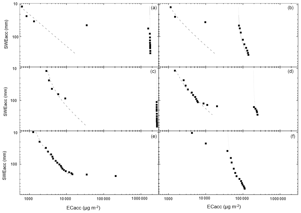
Figure 2 The cumulative ${\stackrel{\mathrm{‾}}{\mathrm{EC}}}_i$ (EC_acc) from top to bottom in the snow pits as a function of accumulated $d_{{\mathrm{SWE}}_i}$, expressed as SWE_acc (mm): (a) pit A, (b) pit B, (c) pit C, (d) pit D, (e) pit E and (f) pit F. The upper dashed line represents a constant deposition EC${}_{\mathrm{y}}^{*}$, and the lower dashed–dotted line represents a constant deposition EC${}_{\mathrm{o}}^{*}$. In pit E there were no snow samples classified as old snow; hence there is no EC${}_{\mathrm{o}}^{*}$ line, while in pit F there were no young-snow samples, and therefore no EC${}_{\mathrm{y}}^{*}$ line.

The visible snow pit stratigraphy described above in Sect. 2.1 can be observed in the pit profiles. At the top, the accumulated EC (EC_acc) as a function of the accumulated d_SWE (SWE_acc) portrays the young-snow layers, whereas in the bottom of the pits the data points represent the old-snow layers (Fig. 2a–f). This pattern (with both young- and old-snow layers) is visible in pits A–D (Fig. 2a–d). These pits also have the enriched LAP layer interleaved between the young- and old-snow layers, indicated by the sharp increase (or steep slope) between the young- and old-snow layers. In the two pits where this general outline is not visible (pit E in Fig. 2e and pit F in Fig. 2f), it can be explained by the fact that pit E extended only to the enriched LAP layer (therefore no old-snow samples), while pit F had essentially no young-snow samples at the time of sampling (therefore pit F starts with the enriched LAP layer).

With the data points for young and old snow appearing rather similar in slope between the pits, the homogeneity is emphasized further by comparing the observations with common effective constants for young and old snow (EC${}_{\mathrm{y}}^{*}$ and EC${}_{\mathrm{o}}^{*}$), respectively. Suitable constants were determined to be close to 50 µg m⁻² mm⁻¹ SWE for young snow and 150 µg m⁻² mm⁻¹ SWE for old snow (see Sect. S4). The resulting deposition using EC${}_{\mathrm{y}}^{*}$ and EC${}_{\mathrm{o}}^{*}$ are superimposed over the observations in Fig. 2a–e as dashed lines for young snow and dotted lines for old snow. These lines then represent the constant deposition of EC as a function of accumulated meltwater in a column according to

$$\begin{array}{}\text{(2)}& {\mathrm{EC}}_{\mathrm{acc}}=\mathrm{constant}\cdot {\mathrm{SWE}}_{\mathrm{acc}}+\mathrm{offset},\end{array}$$

where EC_acc is the accumulated EC mass per square meter, SWE_acc is the accumulated meltwater in L m⁻² (or mm) and the “constant” is the deposition constant. The offsets for young snow are a result of the enhanced observed EC concentration in the top layer, which can numerically be compensated for by “artificially” adding a small value (ΔSWE_acc) to each pit (except pit A), which in essence dilutes the top layer but has a marginal effect on the overall picture. This meant simply rewriting the linear relation above into

$$\begin{array}{}\text{(3)}& {\mathrm{EC}}_{\mathrm{acc}}=\mathrm{constant}\cdot \left({\mathrm{SWE}}_{\mathrm{acc}}+\mathrm{\Delta }{\mathrm{SWE}}_{\mathrm{acc}}\right).\end{array}$$

The ΔSWE_acc amounts were chosen by trial and error to be in multiples of 10 mm for simplicity. The resulting values were 10, 50, 20 and 20 mm for pits B through E in order to explain the apparent offset. A physical interpretation of these numbers may be the loss of water from the surface layer due to evaporation or sublimation, which enhance [EC] in the top layer. For the old-snow layers, snow and EC were numerically removed in the data by subtracting accumulated EC and SWE (including the enriched LAP layer, when present) down to the old-snow layer. This was done such that the first data point satisfies EC${}_{\mathrm{o}}^{*}$. Hence, for old snow $[\mathrm{EC}{]}_{\mathrm{1}}{d}_{{\mathrm{SWE}}_{\mathrm{1}}}/{\mathrm{EC}}_{\mathrm{o}}^{*}={\mathrm{SWE}}_{{\mathrm{acc}}_{\mathrm{1}}}$, where the index (1) represents the top layer of old snow.

By applying the offset values and numerically removing the upper snow layers, we compare the data in Fig. 2a–f in two separate figures (Fig. 3a and b), one where young snow are grouped together and one for old snow. In Fig. 3a, the observed EC_acc is plotted against the EC_acc value if EC${}_{\mathrm{y}}^{*}$ is used. In Fig. 3b the observed EC_acc is plotted against the EC_acc value if EC${}_{\mathrm{o}}^{*}$ is used. Note that for old snow the first data point in the different pits will, by definition, be on the 1:1 line. Nevertheless, the consistency between the pits is striking, and the fact that much of the variation in EC_acc as a function of SWE_acc (or depth in the pit) can be explained by EC${}_{\mathrm{y}}^{*}$ and EC${}_{\mathrm{o}}^{*}$ alone is a very interesting finding.

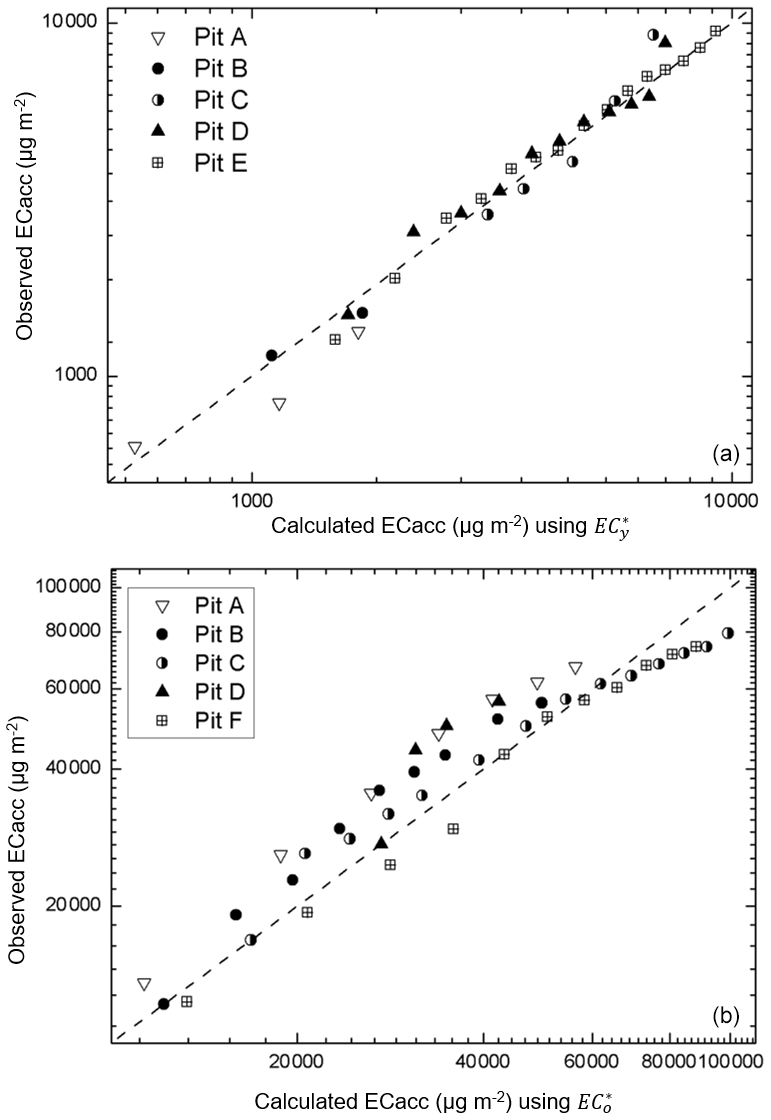
Figure 3 The observed and calculated deposition using the constant deposition EC${}_{\mathrm{y}}^{*}$ for young (a) and EC${}_{\mathrm{o}}^{*}$ for old (b) snow samples. Dashed lines indicate a 1:1 slope.

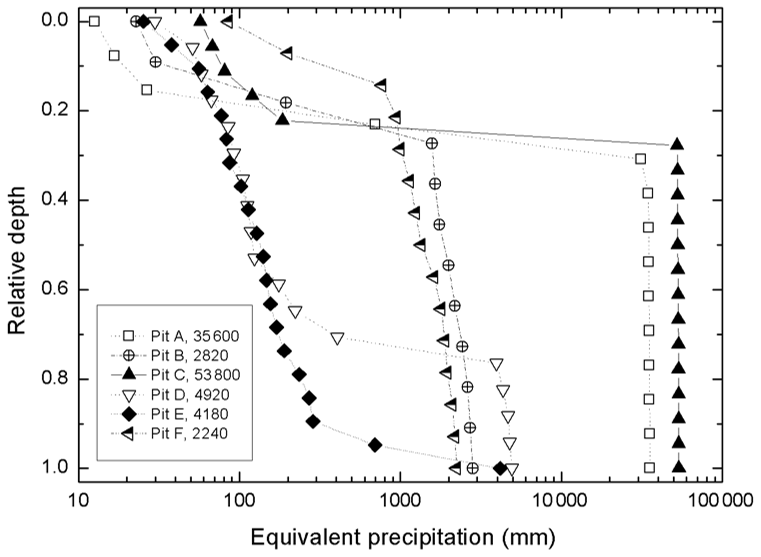
Figure 4 Equivalent precipitation for each pit based on a constant deposition EC${}_{\mathrm{y}}^{*}$ in fresh snow as a function of the relative depth of the pit from top to bottom.

3.2 Enriched LAP layer

Contrary to the observed similarities in the different pits between young and old snow, the samples of the enriched LAP layer do not display similar trends. Instead of being characterized by a common constant, the EC_acc value as a function of SWE_acc in the enriched LAP layer differs by orders of magnitude between the different pit profiles. To explore the enriched LAP layers further, we make use of the constant for young snow EC${}_{\mathrm{y}}^{*}$. Assuming that this is a characteristic value for precipitation during the winter season, we can estimate the required amount of precipitation (SWE_acc) that is needed to explain the observed EC_acc deposition. These derived precipitation amounts for each pit are presented in Fig. 4 as a function of the relative depth from the surface to the bottom of the pit. Using this approach, pit F corresponds to a total equivalent of about 2200 mm in precipitation, whereas pits B, E and D represent 2800, 4200 and 4900 mm, respectively. Pits A and C deviate starkly from the others, with 36 000 and 54 000 mm precipitation. Comparing these derived values to other precipitation estimates allows us to provide a temporal perspective required to explain the observed EC in the pits. Other studies have shown that the annual precipitation is very dependent on altitude level in the Himalayas, and based on the altitude of the glaciers alone one would expect less than about 1000 mm in annual precipitation (Anders et al., 2006; Bookhagen and Burbank, 2010). Based on the changes in snow depth, the local precipitation was estimated using the AWS as described in Sect. 2.2. This analysis gave a snow accumulation of about 600 mm SWE in the 2015–2016 winter season and 700 mm in the 2016–2017 winter season at the location of the AWS. Over the season, a fraction of the snow evaporates or sublimates, possibly accounting for a magnitude of mm d⁻¹ during favorable conditions (Stigter et al., 2018). Further, Mimeau et al. (2019) estimated the sublimation between 12 % and 15 % of the total annual precipitation in the Khumbu Valley, Nepal. This amount might be missed by this method using daily data. Nonetheless, our two precipitation estimates are below the observed annual precipitation of 976 mm in 2012–2013 at 3950 m altitude, about 250 km to the northwest, next to the Chhota Shigri Glacier front (Azam et al., 2016). Measured with an automatic precipitation gauge (i.e., capturing all precipitation forms), the authors found that the majority of precipitation was during the winter season and that the summer monsoon contributed only 12 % to the annual precipitation. Based on these observation estimates and the similarities with our Sunderdhunga AWS precipitation patterns, we estimate that about 800±200 mm is a characteristic annual precipitation amount close to where the pits were dug. If the precipitation amounts derived to explain the deposited EC in each pit is divided by 800 mm, the minimum number of years required to explain the EC observed in the pit is acquired. With this approach it is clear that it would require decades of precipitation to explain the EC in the enriched LAP layers in pits A and C. This is unrealistic, especially when the lower levels in pit F from the previous year are compared. Even the difference in EC amount between pits B, E and D compared to F is much greater than can be explained from aggregating the EC accumulated by 1 year of precipitation in a single melt layer. At the same time, the dry deposition of EC probably accounts for about 7 % of the total deposition. With a dry deposition velocity of EC of 0.3 mm s⁻¹ (Emerson et al., 2018) and an atmospheric concentration of 0.3 µg m⁻³, reported at a similar altitude at the Nepali Pyramid station during the pre-monsoon season (Bonasoni et al., 2010), the dry deposition can be estimated to 2800 µg m⁻² annually, which in comparison to the BC wet deposition, is on the order of 40 000 µg m⁻² annually (obtained by multiplying our 50 µg m⁻² mm⁻¹ with our annual precipitation estimate of 800 mm). Evidently the dry deposition is several orders of magnitude lower than what is encountered in the enriched LAP layers. Thus, this leads us to propose that EC must have been transported laterally in the surface layer during the melt period in the summer of 2016 and converged in the altitude range where the pits were dug. From Fig. 1 it can be seen that the pits were dug in a complex terrain where slopes with an increasing gradient reach up to the summit towards the southwest.

The data and analysis presented above lead us to propose that the old-snow layers observed in pit F from 2015 are the same old-snow layers observed for the pits dug in 2016. The EC equivalent precipitation profile of pit F presented in Fig. 4 suggests that strong melting had taken place already in summer 2015. Hence, the old snow is composed of snow from at least the 2013–2014 season (or perhaps also earlier seasons). Stratigraphy analysis for pit F presented in Svensson et al. (2018) suggested that the snow deposition represented five seasons. The amount of precipitation represented by the EC deposition (cf. Fig. 4) in the old snow is about 2200 mm, which suggests that the EC was deposited over several seasons but less than five seasons. Another strong melt took place in 2016, possibly leading to melting all of the snow from the 2015–2016 season. In addition, during the melting phase, water and snow particulates could be transported down the slopes from areas of the glacier with steep slopes. Because the steepness of the slope decreases towards the valley, this resulted in a convergence of percolated material from areas above the sampling sites. The young snow is likely part of the 2016–2017 winter season that had started to accumulate before the sampling in October 2016 was commenced. This is confirmed by AWS data that indicate intermittent snow events in October 2016. At the AWS location a seasonal snow cover was in place in December 2016.

3.3 Mineral dust fraction in snow

An initial inspection of the mineral fractional absorption on the filters did not reveal any special common pattern in concentration between the different pits, except for the samples of the enriched LAP layer, which appeared to have higher concentrations than the other samples. In Fig. 5, the data are grouped according to the pit stratigraphy classification, and although the absolute range of MD fractions in young-snow samples is very large (5 % to 71 %), the quartile range is only between 32 % to 48 % with a median value of 39 %. The median value for old snow is somewhat larger at 46 %, along with the range and quartiles, which are closer together, from 26 % to 70 % and from 43 % to 50 %, respectively. The range of values for the enriched LAP layer is consistently higher compared to the other two snow types. The median is 78 % with a range and quartiles of 48 % to 95 % and 74 % to 82 %, respectively. Note that from a total of 95 samples only 16 are from the LAP layer. As with EC, MD has the propensity to remain at the snow surface with melting (e.g., Doherty et al., 2013).

Figure 5 Fractional dust absorption remaining after burning the filters during OCEC analysis. The diamonds are individual values for each filter, and the thin extended line represents the arithmetic average. The box and thicker line represent the quartile range and median, respectively. The number of samples is indicated in the figure as n.

Due to the typically heavy loading of material on the filters obtained in the enriched LAP layer, those values should be taken with caution, however. Non-linear effects could skew the resulting light absorption fractions towards larger values, since with a very heavy loading (dark filter) the contribution by remaining particles may be overestimated. This is because the relative contribution by additional light-absorbing material decreases as the amount of material increases on very dark filters. In an extreme case, black layered on top of black will not add any contribution. The larger range of values in young snow compared to old snow is possibly an effect from the geometric thickness of the sampled slabs, which are in young snow generally thinner than in old snow, and a result of the fact that the density of young snow is typically less than the density of old snow. This results in each of the sampled segments in young snow representing less deposition of both water and LAPs and, therefore, presenting a larger variability. Nevertheless, the ensemble of data presents similar median values for both young and old snow. The median of the percentage of the mineral dust absorption f_D value for young- and old-snow samples together becomes 44 %. The specific absorption by minerals is expected to be orders of magnitude smaller than BC (e.g., Utry et al., 2015), and the same is expected with respect to EC. This suggests that the deposition of minerals in the snow is orders of magnitude larger than EC. If we simply scale our characteristic EC constants (EC${}_{\mathrm{y}}^{*}$ and EC${}_{\mathrm{o}}^{*}$) with the median of f_D and the ratio between their specific mass absorption coefficients (MACs), according to

$$\begin{array}{}\text{(4)}& {\displaystyle \frac{f_{\mathrm{D}}}{\left(\mathrm{1}-f_{\mathrm{D}}\right)}}{\displaystyle \frac{{\mathrm{MAC}}_{\mathrm{EC}}}{{\mathrm{MAC}}_{\mathrm{D}}}}{\mathrm{EC}}_{\mathrm{c}}=D_{\mathrm{c}},\end{array}$$

we arrive at a mass concentration for minerals. We use a MAC for BC of 7.5 m² g⁻¹ (Bond and Bergstrom, 2006). The MAC for the minerals is not known and can vary significantly, but for the sake of this test we use a MAC value representative for the mineral quartz of 0.0023 m² g⁻¹ (Utry et al., 2015). If we use these values we arrive at a range of 128–384 µg g⁻¹ of minerals in the snow. This is in range with previous gravimetric observations from the Himalayas (e.g., Thind et al., 2019; Zhang et al., 2018).

3.4 Discussion

Our results indicate that the contribution to light absorption by minerals can be comparable to light absorption by EC in the Sunderdhunga area at about 5 km altitude. This translates into a mass concentration ratio between EC and minerals of more than 3 orders of magnitude. These large ratios are typically not reported for air samples because much of the deposited minerals are likely from local sources. This supports a hypothesis of a positive climate feedback that results in a reduction of snow cover and the exposure to larger sources of minerals.

For the Tibetan Plateau, Zhang et al. (2018) estimated that the retreat of the snow cover could be advanced by more than a week due to LAPs in snow. In their estimates, BC accounted for most of this effect, and dust advanced the melting by about 1 d. The BC concentration in snow used in their calculations were about 1 order of magnitude larger than our derived values from the profiles in the snow pits. This difference can be attributed to the significant contribution of aerosol particle dry deposition in arid regions (Wang et al., 2014), but the range of values presented in their Table 2 reveals a potential problem from sampling surface snow. Post-depositional processes (e.g., sublimation and evaporation, hoar formation, and snow drift) can alter the concentration at a given location relatively fast, which is less of a problem if a deeper layer of the snowpack is investigated instead of solely the surface snow. Simply taking a larger vertical slab is not sufficient as is evident from the melt layer in the present study. The enriched LAP layer in the pits can be studied to characterize the short-term seasonal surface albedo, but the aerosol concentrations cannot be directly related to the deposition. The consistency between pits and different sampling seasons in the integrated deposition profiles above and below the enriched LAP layer show the strength in the data collected from snow pits in comparison to snapshot conditions of surface snow.

4 Conclusions

In this study we aimed at characterizing the observed deposition of EC in the glacier snow in the Sunderdhunga Valley and estimating the contribution from minerals to LAP in the snow. The analysis illustrates that in the sampling area of the Durga Kot and Bhanolti glaciers, the deposition of EC in young snow (from the current winter season) is characterized by approximately 50 µg m⁻² mm⁻¹ SWE water, which is in the range of other observations. The median fraction of light absorption caused by minerals was about 39 % (Q₁=32 and Q₃=48). In old snow (from previous winter seasons), the deposition was characterized by about 150 µg m⁻² mm⁻¹ SWE water. The reason for this difference can simply be due to a larger deposition in the years before sampling was conducted or that more water had the chance to leave the snowpack of older snow. Different from young snow, old snow has had to survive at least one summer season. The median fraction of light absorption was 46 % (Q₁=43 and Q₃=50) by minerals in the old-snow layer. Although the variability within each layer is rather large, the obtained lower median fraction for young snow is consistent with the fact that old snow is more exposed to rock surfaces free of snow during the summer season.

Between these two layers of old and young snow, a clearly visible and very dark layer was present. This layer was most likely a result of strong melting that took place in the summers of 2015 and 2016 as discussed in Sect. 3.2. However, the high concentration of EC found in this layer cannot simply be explained by a collapse of the snowpack vertically, and thus it is concluded that lateral transport of LAPs (including EC and minerals) took place that resulted in a convergence of material in the altitude range of the snow pits. Different from the other two layers (young and old snow), this enriched LAP layer presented large differences with respect to EC content among the different pits. The fraction of light absorption by minerals was the highest of the three layers and was about 80 % (Q₁=74 and Q₃=82).

The profiles of EC and the mineral absorption fraction show good agreement between subsequent years and among different pits. At the same time, the topography in this mountainous region of the Himalayas evidently causes great complexity with respect to the distribution of LAPs in the snow surface layer during periods of strong melt. Although data are limited in spatial and temporal dimensions, our results are useful for large-scale radiation impact assessments of EC deposition and minerals. In small-scale regional studies, however, the effects of complex topography and spatial variability should be considered separately. Future work should further study the mineral dust and its composition in the area, in order to more accurately elucidate dust role in the snow radiation state in this part of the Himalayas.