the Creative Commons Attribution 4.0 License.
the Creative Commons Attribution 4.0 License.
 | 25 Feb 2021
Atmospheric VOC measurements at a High Arctic site: characteristics and source apportionment
Rossana Bossi
Thibaut Lebourgeois
Jacob K. Nøjgaard
Rupert Holzinger
Jens L. Hjorth
Henrik Skov
There are few long-term datasets of volatile organic compounds (VOCs) in the High Arctic. Furthermore, knowledge about their source regions remains lacking. To address this matter, we report a multiseason dataset of highly time-resolved VOC measurements in the High Arctic from April to October 2018. We have utilized a combination of measurement and modeling techniques to characterize the mixing ratios, temporal patterns, and sources of VOCs at the Villum Research Station at Station Nord in northeastern Greenland. Atmospheric VOCs were measured using proton-transfer-reaction time-of-flight mass spectrometry. Ten ions were selected for source apportionment with the positive matrix factorization (PMF) receptor model. A four-factor solution to the PMF model was deemed optimal. The factors identified were biomass burning, marine cryosphere, background, and Arctic haze. The biomass burning factor described the variation of acetonitrile and benzene and peaked during August and September. The marine cryosphere factor was comprised of carboxylic acids (formic, acetic, and C3H6O2) as well as dimethyl sulfide (DMS). This factor displayed peak contributions during periods of snow and sea ice melt. A potential source contribution function (PSCF) showed that the source regions for this factor were the coasts around southeastern and northeastern Greenland. The background factor was temporally ubiquitous, with a slight decrease in the summer. This factor was not driven by any individual chemical species. The Arctic haze factor was dominated by benzene with contributions from oxygenated VOCs. This factor exhibited a maximum in the spring and minima during the summer and autumn. This temporal pattern and species profile are indicative of anthropogenic sources in the midlatitudes. This study provides seasonal characteristics and sources of VOCs and can help elucidate the processes affecting the atmospheric chemistry and biogeochemical feedback mechanisms in the High Arctic.
- Article
(3895 KB) - Full-text XML
-
Supplement
(9175 KB) - BibTeX
- EndNote


The temperature in the Arctic has increased at twice the rate of the global average (IPCC, 2019), a phenomenon known as Arctic amplification. Increased CO2 concentration and sea ice loss are responsible for the majority of this temperature increase (Dai et al., 2019). However, short-lived climate forcers (SLCFs; methane, ozone, black carbon (BC), and aerosol particles) are together responsible for half of the present temperature increase observed in the Arctic (Quinn et al., 2008). Atmospheric aerosol particles are the most important SLCF (due to their scattering, absorbing, and cloud modification properties), but their climate forcing is associated with the largest uncertainty, especially in the Arctic (IPCC, 2019). Ozone is an important photochemical oxidant in the Arctic troposphere. Ozone precursors, e.g., volatile organic compounds (VOCs), nitrogen oxides (NOx), and peroxyacetyl nitrate (PAN), remain poorly characterized in the High Arctic (AMAP, 2015). Photochemical reactions including ozone and VOCs have important implications for the lifetime of methane, a major greenhouse gas. The identification and characterization of processes leading to precursor emissions of aerosols and ozone are therefore needed to improve the assessments of biosphere–aerosol–climate feedback mechanisms.
Several studies have reported on new particle formation (NPF) events involving naturally emitted biogenic VOCs during the summer in the High Arctic. Dall'Osto et al. (2018b) recently demonstrated a negative correlation of NPF events at the Villum Research Station, Station Nord, in northeastern Greenland with sea ice extent. The authors suggested that ultrafine aerosol formation is likely to increase in the future, given the projected increased melting of sea ice (Boe et al., 2009; Bi et al., 2018). Dall'Osto et al. (2017) hypothesized that NPF events during summer on Svalbard were linked to marine biological activities within the open leads and between the pack ice and/or along the marginal sea ice zones, further confirming the same processes are occurring for northeastern Greenland (Dall'Osto et al., 2018a; Nielsen et al., 2019). Open leads and open pack ice emit dimethyl sulfide (DMS) that undergoes atmospheric oxidation leading to methanesulfonic acid (MSA), sulfur dioxide, and ultimately sulfuric acid, which helps form and grow particles (Nielsen et al., 2019). After formation, aerosols grow to sizes that can act as cloud condensation nuclei (CCN) (Ramanathan et al., 2001). VOCs of marine biogenic origin greatly contribute to CCN activity during summer (Lange et al., 2018, 2019). The sources of NPF in the Arctic and its corresponding precursors are a topic of intense research, as uncertainty remains regarding the mechanism of aerosol production. For example, Burkart et al. (2017) found that the condensable vapors responsible for particle growth were more semivolatile than previously observed in the midlatitudes, although they could not identify a source area for these vapors. Aerosol formation is one of the most important factors in determining the surface energy balance in the Arctic. Recently, it was estimated that NPF events could increase CCN concentrations by 2–5-fold over background concentrations (Kecorius et al., 2019). However, parametrization of the processes leading to aerosol formation is still a large source of uncertainty in global radiative forcing predictions (Haywood and Boucher, 2000). The characterization of these gas-phase precursors to particle formation is a key factor for understanding the dynamics of the Arctic troposphere and the corresponding effects on climate.
Ozone is an important pollutant at the surface and a greenhouse gas in the mid-to-upper troposphere. Ozone can perturb radiation fluxes and modify heat transport to the Arctic (Shindell, 2007). In the Arctic, sources of ozone include long-range transport and photochemical production. Ozone and its precursors (VOCs, NOx, CO, and PAN) can be transported from anthropogenic sources in the midlatitudes (Hirdman et al., 2009) and natural boreal forest fire emissions (Arnold et al., 2015), which have been increasing in recent years (Parrish et al., 2012). The major sink for ozone in the Arctic is photochemical loss, followed by minor contributions from dry deposition. Ozone largely controls the oxidative capacity of the atmosphere, as a chief precursor for OH, an oxidant for many compounds, and a major prerequisite for halogen explosion events (Simpson et al., 2007). Halogen explosion events can affect the lifetime and reaction rates for organic gases and the deposition of mercury in the Arctic ecosystem. Photochemical reactions involving VOCs can be a sink (by reactions with ozone) and a source (through reactions with NOx) of ozone. Increased anthropogenic activity in the Arctic (shipping and resource extraction) is expected to increase emissions of both NOx and VOCs (Law et al., 2017). Biomass burning emissions, which are expected to increase in the future, have been shown to increase ozone production by as high as 22 % in the Arctic (Arnold et al., 2015). Ozone levels have consequences for OH radical production, which is the main oxidant of methane, thus largely controlling its lifetime in the atmosphere. Therefore, the characterization of the interactions of ozone and VOCs have implications for climate effects and atmospheric chemistry.
Several factors, including chemical lifetime, local emissions, and long-range transport, govern the mixing ratios of VOCs in the Arctic atmosphere. The chemical lifetime of most VOCs in the Arctic is dependent on the oxidative capacity of the atmosphere, thus there is a strong seasonality (Gautrois et al., 2003). However, due to the low humidity in the Arctic atmosphere, the concentration of OH is low (Spivakovsky et al., 2000). Therefore, halogen and ozone chemistry play an active role in the atmospheric chemistry of VOCs during the spring in Arctic regions (Simpson et al., 2015). However, atmospheric reactions alone seem unable to explain the VOC mixing ratios and dynamics observed at Arctic sites (Grannas et al., 2002; Guimbaud et al., 2002; Sumner et al., 2002), indicating missing sources other than photochemical production. Two potential local sources are the snowpack and the sea surface microlayer. The snowpack also has a major impact on ambient VOCs by uptake–release mechanisms and acts as a matrix for many photochemical and biological processes (Guimbaud et al., 2002; Grannas et al., 2004; Kos et al., 2014). For example, Dibb and Arsenault (2002) demonstrated that the snowpack is a source of formic and acetic acid through the oxidation of ubiquitous organic matter. Furthermore, Boudries et al. (2002) observed emissions from the snowpack to the atmosphere of acetone, acetaldehyde, and formaldehyde, which were explained by photochemical production in the snowpack. Depositional fluxes of methanol were also observed, which they postulated as a source of formaldehyde. These observed gas-phase fluxes had a diurnal cycle following polar sunrise that correlated with the solar zenith angle. Sea surface microlayer emissions are important local sources of atmospheric VOCs, e.g., DMS, formic acid, and acetic acid (Mungall et al., 2017). Sea emissions have a pronounced seasonality because of sea ice preventing air–sea exchange during most of the year in the Arctic. The sea surface microlayer could play a role in the emission of VOCs due to photochemical processes (Chiu et al., 2017; Bruggemann et al., 2018) or heterogenic oxidation (Zhou et al., 2014). For highly water-soluble compounds, the ocean could also be an important sink (Sjostedt et al., 2012). Finally, the transport of VOCs, such as benzene, methane, ethane, propane, and chlorofluorocarbons, has been observed from the midlatitudes to the High Arctic (Stohl, 2006; Harrigan et al., 2011; Willis et al., 2018).
A few studies have reported VOCs in ambient air from Arctic sites with online techniques, usually during short-term campaigns. Hornbrook et al. (2016) utilized nonmethane hydrocarbon measurements to derive time-integrated halogen mixing ratios during the OASIS-2009 campaign at Utqiagvik, AK, (formerly known as Barrow, AK). Mungall et al. (2018) studied the sources of formic and acetic acid at Alert, NU, during the summer of 2016. Sjostedt et al. (2012) and Mungall et al. (2017) performed VOC measurements onboard the CCGS Amundsen in the Canadian Archipelago during the summer of 2008 and 2014, respectively. There have been several campaigns exploring snowpack emissions of VOCs (Boudries et al., 2002; Dibb and Arsenault, 2002; Guimbaud et al., 2002; Barret et al., 2011; Gao et al., 2012). Gautrois et al. (2003) reported long-term VOC concentrations for Alert, NU, where a 7 year time series of VOC mixing ratios has been generated, although with a 9 d time resolution using offline techniques (GC coupled to flame ionization and electron capture detectors). High time resolution measurements are of vital importance for the study of Arctic atmospheric chemistry. For instance, diurnal studies can only be accomplished with a fast-response instrument, as grab samples and time-integrated samples (i.e., adsorbent tubes) will not capture the variability on short enough timescales (de Gouw and Warneke, 2007). Understanding the effects of meteorological parameters on VOC levels requires an instrument response that is shorter than the transient event being observed. Also, flux measurements can only be achieved through fast-responding instrumentation (Müller et al., 2010). The study of short-lived compounds, such as reactive halogen species, and their interactions with VOCs is only possible on short timescales. Finally, global networks have highlighted the need for a quick turnaround in the delivery of atmospheric species for the validation of global atmospheric composition forecasting systems (Schultz et al., 2015). These previous studies call for higher time-resolved and longer measurement campaigns, thus highlighting the importance of long-term high time-resolved measurements of VOCs in the Arctic.
In this study, we report several months of high time-resolved mixing ratios of selected VOCs measured at the High Arctic site Villum Research Station (Villum) at Station Nord (northeastern Greenland). This study aims to provide better insight into the dynamics, seasonal behavior, and potential sources of VOCs in the High Arctic. We accomplish this by combining VOC mixing ratios with meteorological data, air mass back trajectories, and the positive matrix factorization (PMF) receptor model. In Sect. 2, we describe our analytical instrumentation and models in detail. In Sect. 3, we cover the seasonal dynamics of VOCs as well as each factor from the PMF model.
2.1 Field site
The sampling campaign took place at Villum Research Station (Villum), which is situated on the Danish military base Station Nord in northeastern Greenland (81∘36′ N, 16∘40′ W; 24 ). Villum is situated in a region with a dry and cold climate where the annual precipitation is 188 mm and the annual mean temperature is −16 ∘C. The dominating wind direction is southwestern with an average wind speed of 4 m s−1. The sampling took place about 2.5 km southwest of the main facilities of the Station Nord military camp. The sampling location is upwind from the Station most of the time for all seasons (Fig. S1 in the Supplement). An overview of the meteorological data is presented in Fig. S2 in the Supplement. Statistics for meteorological data over the sampling campaign can be found in Table S1 in the Supplement.
Table 1Overview of measured protonated masses included in the PMF analysis. Mean refers to the arithmetic average of the mixing ratio for each compound. Mean, mean LOD, and % < LOD were calculated after quality control of data influenced by local pollution. % QC represents the percentage of data removed due to the quality control procedure (Sect. S2 in the Supplement).
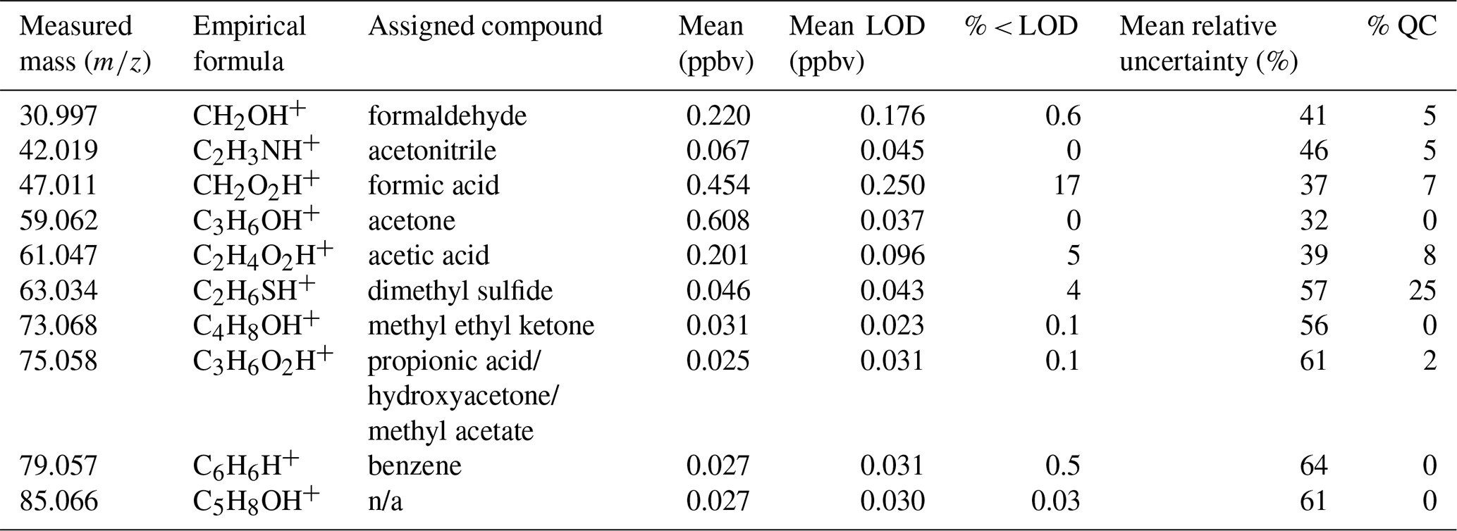
n/a: not applicable.
2.2 Gas-phase measurements and data processing
Gas-phase measurements of VOCs were obtained using a proton-transfer-reaction time-of-flight mass spectrometer (PTR-ToF-MS 1000; Ionicon Analytik GmbH). The measurement campaign commenced after polar sunrise on 4 April and concluded before polar sunset on 28 October 2018. The PTR-ToF-MS was operated with hydronium ion (H3O+) as a reagent ion, a drift tube temperature of 70 ∘C, a drift pressure of 2.80 mbar, and a drift tube voltage of 650 V, leading to an (electric field density of the buffer gas in the drift tube) value of around 120 Td (Townsend). Mass spectra up to = 430 Da were collected at a 5 s single spectrum integration time. The instrument inlet consisted of a PEEK capillary tube heated at 70 ∘C and a built-in permeation unit (PerMasCal; Ionicon Analytik) that emitted 1,3-diiodobenzene, which was used for mass scale calibration. The inlet of the sampling line consisted of Teflon tubing extending through an insulated opening in the roof with a sampling cone at the tip to prevent water and debris from blocking the orifice. Ambient outdoor air was aspirated into the instrument at a rate of 100 mL min−1. Blank measurements were obtained every 4 h for 15 min by automatic switching from the ambient outdoor air to indoor air pumped through a Zero Air Generator (Parker Balston, Part #75–83). Due to technical issues (mainly electrical power failure), measurements were interrupted for short periods ranging from days to weeks in April, June, August, and September. Instrument parameters ( ratio, drift tube temperature, pressure, and voltage) were inspected before and after power failures to ensure proper instrument functionality. Periods with abnormal parameter values were removed. Table S2 in the Supplement summarizes the total number of operational hours for each compound for each month of the campaign.
Data generated by the PTR-ToF-MS were processed with the PTR-MS Viewer software v. 3.2.12 (Ionicon Analytik). Mass calibrations and VOC mixing ratios were calculated by the PTR-MS Viewer based on the reaction kinetics quantification method (Sect. S1 in the Supplement). The instrument quantification was validated against an external gas-phase calibration standard (Apel-Riemer Environmental). A comparison between standard and instrument mixing ratios yielded percent errors that were within the analytical uncertainties (Table 1); therefore, we are confident in the quantification method (Holzinger et al., 2019). The PTR-MS technique allows the observation of species with a proton affinity higher than water; this encompasses most VOCs found in the atmosphere with the important exception of alkanes. It does not allow for a distinction between isomers to be made. Compound names were assigned based on comparison with the libraries from the PTR-MS Viewer, Pagonis et al. (2019), and references therein. Inspection of the mass spectrum yielded 10 protonated masses from which an empirical formula was calculated, and compound names were assigned for nine masses, as discussed in Sect. 3.1. Output files were further processed with MATLAB R2018B for time averaging and blank subtraction. The limit of detection (LOD) for each identified species was calculated as three times the SD (standard deviation) of the blank values for each day. For calculation of the statistics, mixing ratios below LOD were set to the LOD. The data were time-averaged to 30 min means. Uncertainty in VOC measurements accounted for the reaction rate coefficient as well as primary ion counts and blank corrected ion counts; for a detailed description, see Sect. S1. The dataset has been rigorously quality controlled through analysis of particle number size distributions (PNSDs), meteorological data (wind direction and speed), and internal activity logs to remove the influence of local pollution. For a detailed description, see Sect. S2 in the Supplement. Ozone (O3) was measured using an API photometric O3 analyzer M400; the data are quality assured and controlled via standard EN14625:2012 with calibrations every 6 months (Skov et al., 2004, 2020).
2.3 Positive matrix factorization (PMF) analysis
The PMF model was operated using the US EPA PMF version 5.0 software, which uses the second version of the multilinear engine 2 (ME-2) platform (Paatero and Tapper, 1994). The goal of PMF is to identify the number of factors or sources p, the species profile f, and the mass contributed by each factor to each sample. PMF accomplishes this by decomposing a data matrix X into two matrices g and f. The input data matrix X consists of dimensions i and j, where i is the number of samples and j is the measured chemical species. The source profile matrix f is of dimensions p and j. The source contribution matrix g is composed of p and i dimensions. This is expressed in Eq. (1),
where eij is the residual matrix and k is the individual sources. PMF uses measurement uncertainties uij and the residual matrix to minimize the objective function Q in Eq. (2),
where n is the total number of samples and m is the total number of species. There are three versions of the objective function: Qtrue includes all data points, Qrobust excludes outliers, and Qtheo is approximately equal to the number of degrees of freedom. The ME-2 platform performs iterations via the conjugate gradient method until convergence to minimize Q. Each good data point contributes a value of approximately 1 to the value of Q; therefore, Q and the ratio of Qtrue to Qtheo are the goodness of fit parameters for the appropriate number of factors (Paatero et al., 2014).
The following data preparation protocol was developed according to standard practice in the field (Polissar et al., 1998; Reff et al., 2007; Hopke, 2016), which allows PMF analysis to be performed effectively. In certain cases discussed here, the dataset was modified before modeling via PMF. Data with concentrations below the LOD were replaced with a value equal to half of the LOD. The associated uncertainty was set to of the LOD. Missing concentrations from a sample were replaced with the median concentration of the dataset and the uncertainty was set as a multiple (3) of the median concentration (Polissar et al., 1998; Reff et al., 2007). It is worth noting that the operational protocols used to estimate the uncertainties and treatment of data are based on extensive testing to find an approach that provided useful results (Hopke, 2016). Numerous sensitivity runs were performed to evaluate the validity of this data preparation protocol including varying the treatment of data below the LOD (replacing with half of the LOD or leaving as is), the treatment of missing values (removing the sample or replacing missing species with the median), the treatment of the uncertainty matrix, the number of species included in the model (species were systematically removed or added to observe their influence on the model solution), the threshold values for species categorization, and the number of factors. Each variation of the input data, of course, produced a unique solution. However, the overall shape of the time series and factor contributions profile were consistent with the solution present in this study. The optimal model solution, for the configuration present here, was therefore deemed robust to these variations of the input data and provided acceptable diagnostics.
Two methods for evaluating modeling uncertainty in PMF were performed: bootstrapping (BS) and displacement of factor elements (DISP) (for a description, see Paatero et al. (2014)). BS uncertainty includes effects from random errors and partially includes the effects of rotational ambiguity. DISP explicitly captures uncertainty from rotational ambiguity (Brown et al., 2015). Another method of estimating rotational ambiguity is the Fpeak function. Fpeak evaluates Q under different rotational strengths; in this study, Fpeak strengths range from −5 to 5 in intervals of 1 and from −1 to 1 in intervals of 0.1.
2.4 Ancillary data
Meteorological data including temperature, relative humidity, wind speed, wind direction, pressure, radiation, and snow depth were generated by an automatic weather station placed ∼ 44 m away from the measurement site. Using the local wind direction and wind speed, a conditional probability function (CPF) was calculated using the source contributions for each factor. CPF is defined as CPF = , where mθ is the number of occurrences that a source contribution exceeds a predetermined threshold criterion (75th percentile) while arriving from a wind sector and nθ is the total number of occurrences that wind arrived from the same wind sector. A wind sector was defined as 30∘ and wind speeds below 0.5 m s−1 were excluded to account for uncertainty in wind direction at low wind speeds. Daily polar gridded sea ice concentrations for the measurement period were obtained through the Nimbus-7 SMMR and DMSP SSM/I-SSMIS passive microwave data (Cavalieri et al., 1996). Time series of local sea ice concentrations were calculated from the gridded daily average sea ice concentrations (%) by masking an area of ± 2∘ longitude and +8∘4∘ latitude around Villum (Greene et al., 2017; Greene, 2020).
2.5 Back trajectory analysis
To investigate source regions, the R package openair (Carslaw and Ropkins, 2012) was utilized to produce a potential source contribution function (PSCF). Trajectories in openair were calculated using the HYSPLIT model (Draxler and Hess, 1998; Rolph et al., 2017) at 100 m altitude and 120 h backward in time using Global NOAA-NCEP/NCAR reanalysis data archives at a 2.5∘ resolution. A PSCF, shown in Eq. (3), calculates the probability that an emission source is located in a grid cell of latitude i and longitude j on the basis that emitted material in the grid cell ij can be transported along the trajectory and reach the receptor site:
where nij is the number of times a trajectory has passed through grid cell ij and mij is the number of times that a concentration was above a certain threshold value, in this case, the 90th percentile. To account for uncertainty in cells with a small number of trajectories passing through, a weighting function was applied (Carslaw and Ropkins, 2012).
3.1 VOC temporal patterns and mixing ratios
The 10 selected masses monitored by the PTR-ToF-MS and their assignments to species names are presented in Table 1. Assignments are made by choosing the most plausible contributions to an observed mass but each measured ion may have contributions from several different isomeric molecules. The assignment of masses in the table to protonated molecules of formaldehyde, acetonitrile, formic acid, acetic acid, and benzene appears to be unproblematic as no meaningful alternatives are found. For the remaining molecules, alternative assignments are possible. The mass assigned to acetone could be propanal as well, but propanal has a shorter atmospheric residence time and acetone is known to be one of the dominating VOCs observed in the atmosphere (Jacob et al., 2002). Further, it has been found to have sources in the Arctic (Guimbaud et al., 2002). The mass assigned to DMS could be ethanethiol as well, but the large marine source of DMS makes it the most plausible assignment. Methyl ethyl ketone is isomeric with butenal, but being the second most abundant ketone in the atmosphere with, among others, apparently an oceanic source (Brewer et al., 2020) it appears to be the best assignment. C3H6O2 may stem from propionic acid but also hydroxyacetone, methyl acetate, and ethyl formate. While it seems unlikely that ethyl formate could give a major contribution to this signal, the other three species are all plausible candidates. Low molecular weight organic acids are commonly found in the atmosphere (Lee et al., 2009), methyl acetate has been found in emissions from biomass burning (Andreae, 2019), and hydroxyacetone is known to be formed by the atmospheric degradation of isoprene (Karl et al., 2009). For what concerns the C5H8OH+ ion we prefer not to make an assignment; possible isomers include, among others, pentenals and pentenones.

Figure 1Time series of mixing ratios (ppbv) for (a) formaldehyde, (b) acetonitrile, (c) formic acid and acetic acid, (d) acetone and MEK, (e) DMS and C3H6O2, and (f) benzene and C5H8O during the entire measurement period.

Figure 2Time series for (a) formic acid, acetone, acetic acid, and radiation and (b) MEK, formaldehyde, C3H6O2, DMS, and radiation during the period 22 June–9 August displaying the diurnal profile for each species.
For the 10 selected VOCs, the time series of mixing ratios during the entire measurement period are displayed in Fig. 1a–f. During the spring (April–May), certain compounds (benzene and C5H8O) exhibited a maximum and thereafter a decreasing pattern, similar to the timing and profile of the Arctic haze phenomenon. During the spring, compounds did not display a diurnal profile except for acetic acid (Fig. S3 in the Supplement), while in summer (June–August), oxygenated volatile organic compounds (OVOCs) revealed a diurnal cycle that closely follows radiation (Fig. 2 and Fig. S4 in the Supplement). Compounds of nonphotochemical origin (benzene and acetonitrile) also displayed a slight diurnal pattern, which could possibly be due to entrainment from aloft (Fig. S4 in the Supplement). Interestingly, several compounds (formaldehyde, formic acid, and acetone) peaked in the spring with decreasing levels until the summer, when a diurnal pattern following sunlight was observed (Figs. 1 and 2 and Fig. S4 in the Supplement). During the autumn (September–October), all compounds were low except for acetone and acetonitrile (Fig. 1) and only acetic acid displayed a diurnal profile (Fig. S5 in the Supplement). The levels, seasonal patterns, and comparisons with other studies of these compounds are discussed below.
Formaldehyde, formic acid, methyl ethyl ketone (MEK), and acetone, and to a lesser extent acetic acid and C5H8O, displayed a decreasing pattern in the spring. For formaldehyde, formic acid, acetic acid, acetone, MEK, and C3H6O2, a diurnal variation was observed in the period July–August, with peak mixing ratios occurring around midday (Fig. 2 and Fig. S4 in the Supplement), highlighting their dependence on sunlight. Acetone showed the highest mean mixing ratio ± SD (0.608 ± 0.196 ppbv). The mean mixing ratios of acetone measured at Utqiagvik, AK, during the OASIS-2009 field campaign (March–April 2009) were 0.900 ± 0.300 ppbv (range of 0.364–2.21 ppbv) (Hornbrook et al., 2016) and in the Canadian Archipelago in August–October they were 0.424 ppbv (Sjostedt et al., 2012), which is within the same range observed at Villum (0.608 ± 0.196 ppbv; Table 1). The average mixing ratio of formaldehyde in the present study (0.220 ± 0.128 ppbv) is similar to those measured at Utqiagvik, AK, (0.204 ppbv) and Alert, NU, (0.166 ppbv) in March–April (Grannas et al., 2002; Barret et al., 2011). The formic acid (0.454 ± 0.371 ppbv) and acetic acid (0.201 ± 0.149 ppbv) mean mixing ratios were within the range of those measured at Summit, Greenland, (0.4 ppbv) by Dibb and Arsenault (2002), although considerably lower than those measured by Mungall et al. (2018) during the early summer at Alert, NU, (formic acid 1.23 ± 0.63 ppbv, acetic acid 1.13 ± 1.54 ppbv). MEK displayed a mean mixing ratio of 0.031 ± 0.021 ppbv, which is slightly lower than the median concentrations of 0.190 ppbv measured in March–April 2009 at Utqiagvik, AK, (Hornbrook et al., 2016) and 0.054 ppbv measured at Alert, NU, in April–May 2000 (Boudries et al., 2002).
The two main nonoxygenated compounds measured were acetonitrile and benzene. Benzene mixing ratios followed the expansion of the polar dome with high mixing ratios in the spring period and the lowest in the summer period (Fig. 1f), similar to sulfate and BC measured (Massling et al., 2015; Skov et al., 2016) and accumulation mode aerosols (Lange et al., 2018). The mean mixing ratio of benzene measured at Villum was 0.027 ± 0.016 ppbv, which is a factor of two higher than those measured in the Canadian Archipelago (0.013 ppbv) by Sjostedt et al. (2012). Benzene has shown a seasonal pattern at Alert, NU, with a higher mixing ratio in winter due to no or limited photochemistry and long-range transport from lower latitudes (Gautrois et al., 2003). They reported mean winter and summer mixing ratios of 0.200 and 0.034 ppbv, respectively; when compared to the present study there is good agreement during the summer. Acetonitrile followed a similar pattern to benzene during the spring with decreasing values as well as exhibiting minima in the summer and maxima during the autumn (Fig. 1b). The mean mixing ratio of acetonitrile observed at Villum is 0.067 ± 0.025 ppbv, which is a factor of two higher than that reported by Sjostedt et al. (2012) (0.030 ppb). The range of acetonitrile mixing ratios (0.023–0.156 ppbv) corresponds to the upper and lower limits of background levels over the Atlantic Ocean (0.10–0.15 ppbv) reported by Hamm et al. (1984) and Hamm and Warneck (1990). The main source of acetonitrile in the atmosphere has been found to be biomass burning (Singh et al., 2003).
DMS was the only sulfur-containing compound detected, with a mean ± SD of 0.046 ± 0.043 ppbv. The mixing ratios of DMS observed in this study are a factor of two lower than those reported by Sjostedt et al. (2012) (0.093 ppbv). DMS mixing ratios were near LOD during the spring and autumn; however, they were at significantly elevated levels during the summer periods of sea ice melt (Figs. 1e and 2).
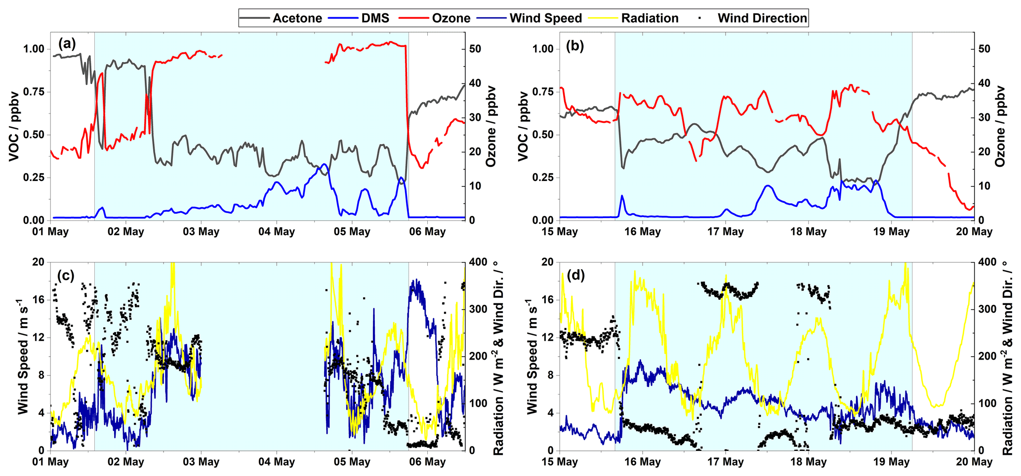
Figure 3(a, c) The first period of elevated DMS mixing ratios (1–5 May). (b, d) The second period of elevated DMS mixing ratios (15–19 May). Panels (a) and (b) show the mixing ratios of acetone and DMS (left axis), and ozone (right axis); panels (c) and (d) show the wind speed (left axis) and radiation and wind direction (right axis). The shaded area represents episodes of elevated DMS mixing ratios.
3.2 Springtime VOC correlations
Elevated DMS mixing ratios were observed for two short periods of a few days' duration in May (1–5 and 16–19 May), when DMS mixing ratios increased an order of magnitude from ∼ 0.02 to > 0.2 ppbv (Fig. 3a and b). In May, most of the ocean surrounding Villum is still frozen. However, satellite images from the area (available at http://ocean.dmi.dk/arctic/nord.php, last access: 12 January 2021) showed that there were open leads in the frozen sea surface. Back trajectory calculations (Fig. S6a and b in the Supplement) confirmed that during the DMS emission episodes, the air masses experienced extensive surface contact and traversed near areas containing open leads (as identified from satellite images) before reaching the station. During DMS emission episodes, the acetone mixing ratios decreased correspondingly. Sjostedt et al. (2012) found moderate anticorrelation (R=0.37, ) for DMS with acetone. Minimum values of acetone were observed when DMS reached its maximum values, and the short photochemical lifetime of DMS suggests a localized biological sink for acetone associated with the production of DMS. Certain microorganisms can consume acetone as well as produce DMS from DMSP (Taylor et al., 1980; Kiene et al., 2000). At Villum, the relationship between acetone and DMS showed seasonal changes with a moderate negative correlation in April (R = −0.55), a weak positive correlation in July (R = 0.23), and a moderate negative correlation in September (R = −0.68). Possible reasons for these variations may be changes in the biological conditions of the seawater, photochemical activity, and source regions. Pearson correlation coefficients for chemical species, radiation, and temperature for April, July, and September are tabulated in Tables S3–S5 in the Supplement, respectively.
As illustrated in Fig. 3a and b, acetone is anticorrelated with ozone during periods of elevated DMS. This relationship is particularly evident during situations with abrupt changes in the mixing ratios of the species as on 1, 2, and 5 May. These changes in mixing ratios are accompanied by a change in meteorological conditions, illustrated here by changes in wind speed and to a less extent by wind direction (Fig. 3). Guimbaud et al. (2002) found a similar relationship between acetone and ozone during different field campaigns at Alert, Canada, with elevated acetone levels during ozone depletion episodes accompanied by a concomitant decrease in the propane mixing ratios. However, it was found that the increase in acetone could not be explained by gas-phase chemistry but possibly by photochemically induced emissions from the snowpack. This phenomenon was also observed by Boudries et al. (2002). The anticorrelation between ozone and acetone observed at Villum may also be explained by a similar influence of photochemistry that causes destruction of ozone as well as the formation of acetone by gas phase and surface reactions. Also, the possible influence of vertical air exchange must be considered. During pristine atmospheric conditions at Villum, ozone is destroyed but not produced within the boundary layer due to low NOx concentrations (Nguyen et al., 2016). Exchange with the free troposphere will lead to increases in ozone concentrations and possibly reductions in acetone concentrations at ground level due to dilution by air from aloft with a lower acetone concentration. The anticorrelation between ozone and acetone supports the hypothesis that acetone is not brought down from aloft to a significant extent but has surface or boundary layer chemistry as its main source.
During the summer, the behavior of acetone is different. In addition to the previously mentioned dependence on the diurnal variations of sunlight (Fig. 2 and Fig. S4 in the Supplement), providing strong evidence of a local photochemical source, a positive correlation with ozone was observed. In June, an anticorrelation is still seen, but in July and August the two species are correlated (R = 0.69 for July and R = 0.46 for August). The fact that ozone is also positively correlated to other OVOCs (particularly formaldehyde, R = 0.86 for July) suggests that the correlation is due to the influence of transport of air containing ozone and acetone formed by the photochemical degradation of air pollutants. During the summer period, acetone is correlated with acetonitrile (R = 0.73 for June–August); in September and October this correlation becomes very strong (R = 0.96). Acetonitrile is considered an atmospheric tracer of biomass burning because the global budget of this compound, as previously mentioned, is dominated by emissions from biomass burning (Holzinger et al., 2001). Thus, biomass burning and atmospheric degradation of biomass burning products seem to be important sources of acetonitrile and acetone during this period. The correlation with ozone is also positive during these months, most likely because the photochemistry of biomass burning emissions is also a source of ozone brought to Villum. The different temporal patterns and correlations suggest the behavior and sources of VOCs in the Arctic are seasonally dependent. Therefore, a detailed, statistical investigation of the sources affecting VOC levels is warranted.
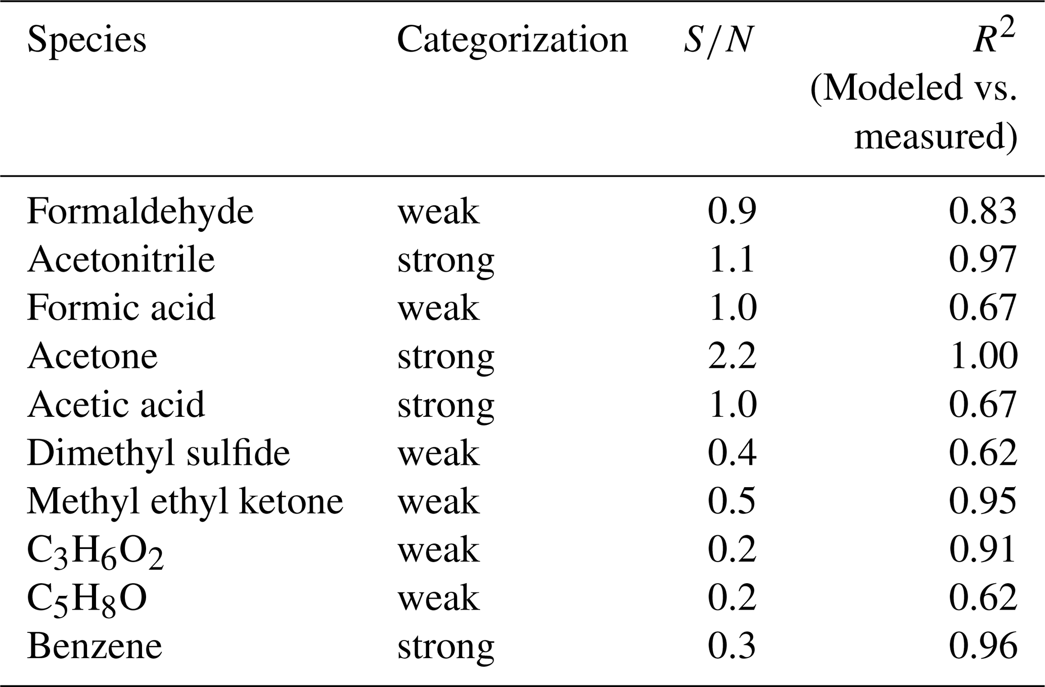
Table 2Input species for the PMF model along with species categorization, , and R2 values for modeled vs. measured values.
3.3 Source apportionment via PMF
VOCs exhibited distinct temporal patterns that are seasonally dependent and suggest different processes contributing to ambient mixing ratios. Therefore, the source apportionment model, PMF, was employed to provide an in-depth examination of these VOC sources. The base model was executed 100 times with a random start seed. Species were categorized based on their . Species with an ≥1, 0.2 < < 1, < 0.2 were categorized as “Strong”, “Weak”, and “Bad”, respectively. The uncertainties of Weak species were tripled, and Bad species were excluded from the analysis. Two species deviated from this categorization; benzene ( = 0.3) was classified as Strong since it serves as a tracer for anthropogenic emissions from fossil fuel combustion and formic acid () was classified as Weak since there was substantial variability of blank measurements in the spring. Rather than down-weighting spring samples, the entire dataset for formic acid was down-weighted to minimize bias for the spring period. The species included in the analysis were those shown in Table 2. Expanded uncertainties for model input were estimated as described in the Sect. S1 in the Supplement. The two periods of elevated DMS mixing ratios were removed from the model input matrix since these periods were considered an anomaly compared to the rest of the measurement period (appearance of open leads, wind direction directly from these leads, and air masses with extensive surface contact). Therefore, these periods violated one of the assumptions of PMF, namely that sources do not change significantly over time or do so in a reproducible manner. The inclusion of these two periods did not improve model performance. Instead, we argue that their exclusion allows us to model the ambient behavior of VOCs devoid of episodic influence due to certain meteorological conditions.
A four-factor solution was deemed optimal based on ratios, R2 values between modeled and measured mixing ratios, and physical interpretation of the factor time series and profiles. Figure S7 in the Supplement displays the ratios against the factor number. Increasing the factor number from 2 to 3 produces the largest decrease in the ratio, which is often taken as the optimal solution for the number of factors. However, the mean R2 values for the three-factor solution (0.8) were lower than for the four-factor solution (0.85) and the physical interpretation of the four-factor solution yielded more robust analysis. Therefore, a four-factor solution was deemed optimal. The large discrepancy between Qtrue and Qtheo can be explained by the large analytical uncertainties (32 %–64 %; Table 1), which is due to the extremely low mixing ratios observed, causing Qtrue to be small, the large number of samples that produce a large Qtheo, as well as covariation in the species (see Sect. 3.1). While these uncertainties are high, they are reasonable for a kinetic quantification of organics at these instrument parameters and extremely low mixing ratios based on Holzinger et al. (2019).
Displacement on the four-factor solution yielded no errors in the model and zero factor swaps, illustrating the solution is valid and free of rotational ambiguity. Bootstrapping was performed for 100 runs and mapped > 85 % of the boot factors to the base factor. This high percentage indicates the model solution is free of random error. Variations of the Fpeak strength consistently returned the lowest change in Q at Fpeak = 0, indicating the model is free of rotational ambiguity. The inspection of G-space plots produced no visible correlations between factors. Together these error estimation methods show the model solution is robust, valid, and free of random errors and rotational ambiguity.
Based on their chemical composition and their temporal variation, the four factors were assigned to likely sources, including biomass burning, marine cryosphere, background, and Arctic haze, which is explained in detail below.
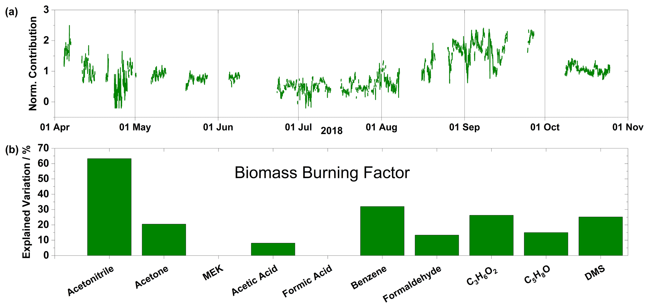
Figure 4(a) Time series of normalized contributions and (b) species profile for the biomass burning factor. Factor contributions are normalized to give a mean contribution of unity.
3.3.1 Biomass burning factor
The most prominent species in the profile of the biomass burning factor are acetonitrile, explaining 63 % of the variation, and benzene, explaining 33 % of the variation (Fig. 4b). As mentioned above, acetonitrile is a characteristic tracer for biomass burning emissions. Biomass burning is also an important source of benzene, with an estimated global strength of about half of the anthropogenic sources (Lewis et al., 2013) and a source of methyl acetate (Andreae, 2019), one of the C3H6O2 isomers. The chemical species profile (Fig. 4b) of this factor, therefore, points to a biomass burning source. The time series (Fig. 4a), shows this factor decreasing in the spring to a minimum in the summer and slowly increasing to a maximum at the beginning of September. The decrease in the spring is reflective of decreasing concentrations of benzene and acetonitrile. In the case of benzene this can be ascribed to anthropogenic emissions during this period as the polar dome is expanded during winter and spring, allowing for emissions to be entrained from the midlatitudes. In the case of acetonitrile, the reason is more uncertain; there are anthropogenic sources of acetonitrile, particularly wood burning for residential heating and solvent use (Languille et al., 2020), but they appear to be of very minor importance compared to forest fires (de Gouw et al., 2003). The height of the biomass burning season in North America and northern Eurasia is July (Lavoue et al., 2000), although due to the contraction of the polar dome during summer, minimum contributions from this factor are observed. Increased areas of open water in the Arctic also act as a sink for acetonitrile during the summer (de Gouw et al., 2003). The biomass burning factor peaks in August/September, when the polar dome starts to expand, thus allowing biomass burning emissions to reach the High Arctic.
To examine the geographical origin of this factor, air mass back trajectories from the HYSPLIT model were calculated every hour during the peak of the biomass burning factor (15 August–15 September 2018) and extending 336 h (two weeks) backward in time. The trajectory length of 2 weeks was selected to account for the long lifetime of acetonitrile. Active fires during the period 15 August–15 September 2018 were provided by NASA's Fire Information for Resource Management System (FIRMS) (Schroeder et al., 2014). Active fires occurring within 1 h and 1∘ latitude/longitude of a trajectory endpoint were used to access the influence of active fires on the biomass burning factor. While there was evidence of active fires in North America and Eurasia occurring near a trajectory endpoint within 1 h, the uncertainty of a trajectory with a length of 336 h is quite large (Stohl, 1998). Therefore, no meaningful conclusions can be drawn from this analysis other than that the transport time of emissions influencing the biomass burning factor is greater than 2 weeks and that we are unable to capture these emissions with the current trajectory models with any confidence.
The influence of biomass burning was observed at other High Arctic sites during this period. Lutsch et al. (2020) used Fourier-transform infrared spectroscopy (FTIR) measurements of CO, HCN, and ethane at several High Arctic sites coupled with aerosol optical depth data and the GEOS-Chem model to detect the influence of wildfires and attribute their sources. They observed fire-affected enhancements in the tropospheric CO column at Eureka, NU, from 9 to 25 September 2018, and at Thule, Greenland, from 24 August through 26 September 2018. The GEOS-Chem simulated the source regions for the fire-affected enhancements in the tropospheric CO column measurements to be boreal forests in North America and Asia at both sites (Lutsch et al., 2020). These observations of biomass burning at other High Arctic sites are in good agreement with the biomass burning factor presented here, adding robustness to this factor assignment that can offer insight into the geographical origins of the biomass burning factor.
Biomass burning is known to be an important source of BC, and it has been estimated to account for about 35 % of the BC emissions in the Northern Hemisphere (Qi and Wang, 2019). Despite this, the observed time profile of BC (not shown) at Villum did not show an increase during the autumn of 2018. This is likely to be explained by the fact that the emissions from biomass burning sources have been transported over long distances with corresponding long transport times (> two weeks), as BC is removed much faster from the atmosphere than acetonitrile due to wet deposition. The atmospheric residence time of BC is below 5.5 d according to a recent estimate (Lund et al., 2018), while that of acetonitrile is several months (de Gouw et al., 2003). Using meteorological parameters calculated along the trajectory path using HYSPLIT (see above), the mean accumulated precipitation for the peak of the biomass burning factor was 14 mm. Raut et al. (2017) used a combination of in situ observations from aircraft, satellite remote sensing, and modeling simulations to calculate the transport efficiency of BC during 2012. They concluded that the transport efficiency of BC was low (< 30 %) when the accumulated precipitation was large (5–10 mm). These previous observations combined with the accumulated precipitation data along each trajectory during the peak of the biomass burning factor support the lack of BC loading during this time. While biomass burning is a source of BC globally, which is expected to increase in the future (Westerling et al., 2006), the results presented here indicate that meteorological parameters encountered during transport can play a role in the levels observed in the High Arctic atmosphere. While biomass burning emissions may increase in the future, increased precipitation patterns might counterbalance this increase, although more research is needed to elucidate the relationship between these feedback mechanisms.
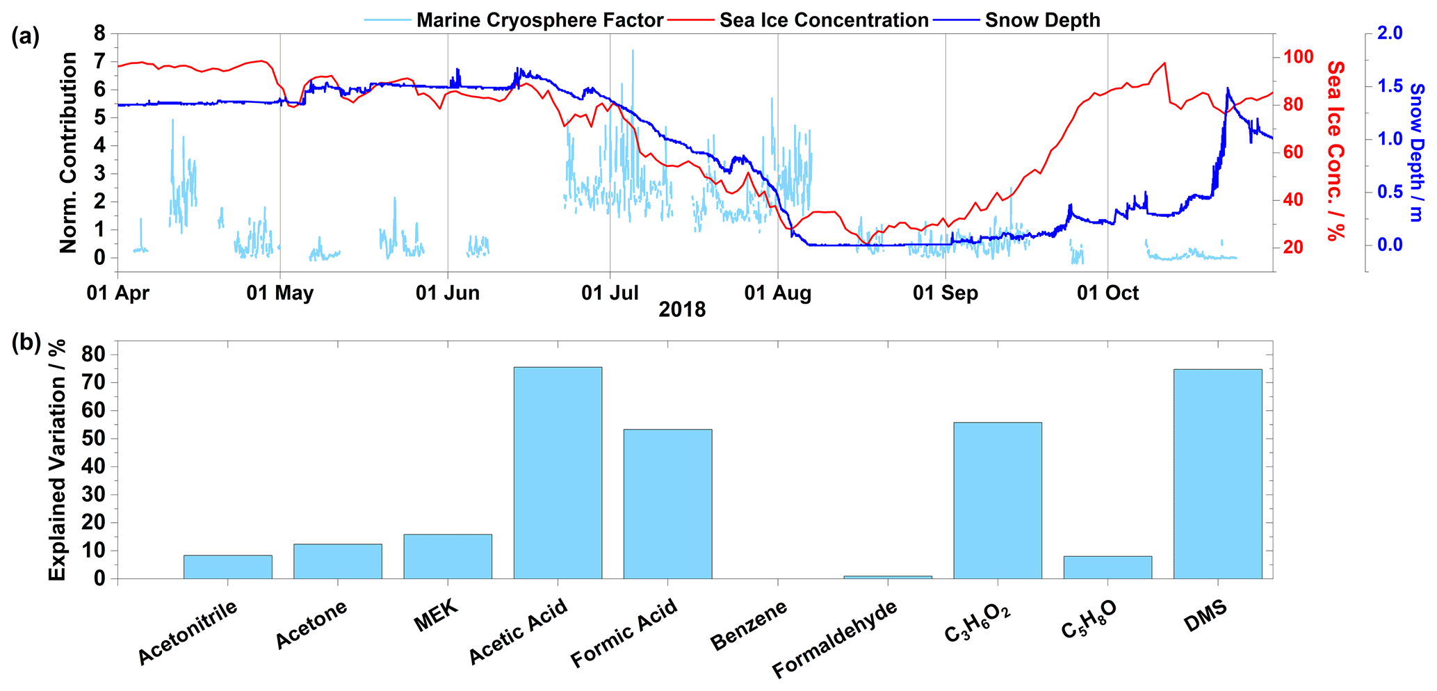
Figure 5(a) Time series of normalized contributions in light blue (left axis), sea ice concentrations in red (right axis), and snow depth in blue (right axis). (b) Species profile for the marine cryosphere factor. Factor contributions are normalized to give a mean contribution of unity.
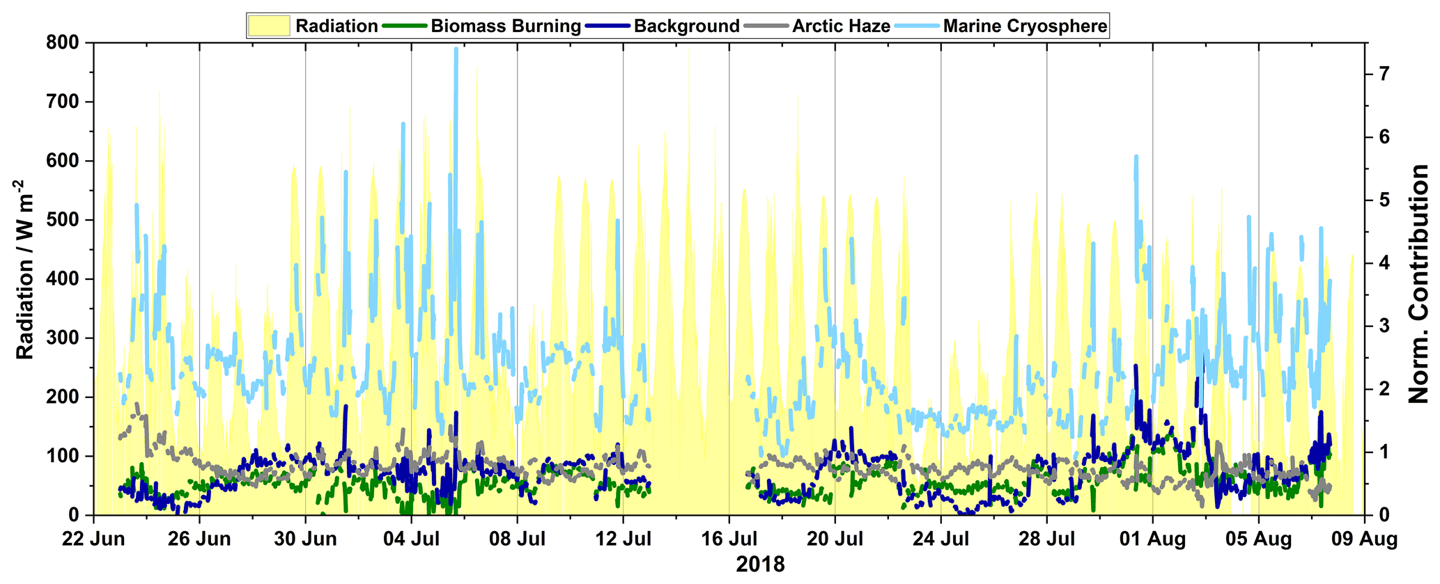
Figure 6Time series of the four factors from 22 June–9 August displaying the diurnal profile together with radiation.
3.3.2 Marine cryosphere factor
The marine cryosphere factor was characterized by formic acid, acetic acid, C3H6O2, and DMS, explaining over 50 % of the variability of each of these compounds (Fig. 5b). The contribution of this factor is near zero in the spring and autumn and reaches a maximum during the summer months (Fig. 5a). This factor shows an enhanced diurnal variation with a correlation to sunlight during the summer months (Fig. 6). The high content of DMS points to a marine origin of this factor, while carboxylic acids have been demonstrated to be emitted from the snowpack (Dibb and Arsenault, 2002). An analysis of snow depth and sea ice concentrations ( ± 2∘ longitude and +8∘4∘ latitude area around Villum) illustrates that the onset of this factor coincides with the snowmelt and sea ice decline. Therefore, a combination of marine and cryosphere sources appears to contribute to the species observed in this factor. The C3H6O2 is in this case assigned to propionic acid as the alternative isomers seem less probable considering their typical origins (biomass burning for methyl acetate and isoprene oxidation for hydroxyacetone).
The sources of the organic acids are much less well characterized than those of DMS; in fact, model simulations have not been able to reproduce the mixing ratios of formic and acetic acid, particularly in the Arctic and northern midlatitudes (Paulot et al., 2011; Mungall et al., 2018). As the lifetimes of formic acid and acetic acid against photochemical oxidation by reaction with the OH radical are relatively long (about 25 and 10 d, respectively, for [OH] = 106 ), dry and wet deposition is thought to be the main removal pathways (Seinfeld and Pandis, 2016). The estimated globally averaged atmospheric lifetimes against deposition for both formic and acetic acid in the boundary layer are between 1 and 2 d (Paulot et al., 2011). Thus, it is unlikely that direct long-range transport plays a relevant role in determining the mixing ratios of these species at Villum. Analyses of 14C isotopes in formic and acetic acid in air and rainwater have shown that outside of urban and semiurban areas the dominating (> 80 %) source is modern carbon (Glasius et al., 2001). These analyses are consistent with model simulations showing that atmospheric oxidation of biogenic hydrocarbons is the largest source (Paulot et al., 2011; Millet et al., 2015). Even though vegetation in the High Arctic is sparse, contributions from precursor emissions or direct emissions of formic acid and acetic acid from vegetation cannot be excluded, as discussed by Mungall et al. (2018). Emissions from the soil are also a possible but highly uncertain source of these species (Mungall et al., 2018). However, the marine cryosphere factor is largely absent when snow is completely melted, exposing the bare ground and vegetation to the atmosphere, thus soil emissions and vegetation are improbable sources of these compounds. Instead, enhancements in these species and this factor is observed during periods of snowmelt and sea ice melt.
A comparison of the contribution of the marine cryosphere factor to sea ice concentration, calculated as described in Sect. 2.3, and snow depth can further shed light on the origin of this factor (Fig. 5a). Periods of high contributions and diurnal pattern by the marine cryosphere factor started on 22 June (Fig. 6), when the local sea ice concentration and snow depth are starting to decline. Diurnal patterns were observed during this period of melting (Figs. 5a and 6). This continued until 9 August, when the measurements were interrupted due to technical issues. When measurements resumed on 16 August, the contribution from the marine cryosphere factor had returned to the low levels found during springtime. Note that instrument parameters were monitored before and after interruptions to ensure proper functionality of the instrument, and periods that deviated from nominal values were removed. The marine cryosphere factor appears to not be strongly dependent on the extension of the open sea, as sea ice concentrations/extensions reach a minimum and consequently the open sea area reaches a maximum by the beginning of September, but rather depends on active melting of snow and sea ice. Thus, it seems that emissions of VOCs from melting snowpacks and newly exposed sea ice areas could offer a viable explanation for the observed dependence of this source.
Previous work has shown that emissions from the sea in the Arctic area can be caused by a surface microlayer enriched in organic substances that acts as a source of formic acid and other oxidized VOCs (Mungall et al., 2017). This occurs either via heterogeneous chemistry or by photochemically driven reactions within the surface layer (Vlasenko et al., 2010; Chiu et al., 2017). Mungall et al. (2017) performed factor analysis of VOCs in the Canadian Archipelago and found four factors. One factor (ocean factor; containing formic acid, isocyanic acid, and oxo-acids) was highly correlated with dissolved organic carbon (DOC), fluorescent chromophoric dissolved organic matter (fCDOM), and radiation. However, DMS was poorly correlated with this factor. They concluded the source to be photochemical or heterogeneous oxidation from sources on the sea surface microlayer. While formic and acetic acid, as well as the carbonyl compounds, show daily variations correlating with radiation, as mentioned above, DMS shows a less clear correlation. The emission of DMS from the open ocean has been demonstrated to be dependent on horizontal wind speed (Bell et al., 2013), although the variation of the marine cryosphere factor seems to not be driven mainly by the dependence on horizontal wind speed (R = −0.04). Marine microorganisms produce DMS (Stefels et al., 2007; Levasseur, 2013), and given the distance of the measuring site from open water (taking sea ice into account the station is approx. 25 km from open water), it is proposed that the majority of DMS produced is already oxidized to MSA and other products when it reaches the station. The presence of gas-phase MSA has been indicated by the observation of the methanesulfonate ion, which has been previously measured in the particle phase at Villum in February–May 2015 (Dall'Osto et al., 2018b; Nielsen et al., 2019).
Several studies have demonstrated the emission of VOCs from the snowpack. Gao et al. (2012) observed the photoenhanced release of VOCs from both Arctic and midlatitude snow, and Grannas et al. (2002) obtained similar results by applying a box model to simulate observed emissions of carbonyl compounds from an Arctic surface layer at Alert. They found that diel cycles of carbonyl compounds are impacted by snowpack exchange characterized by nighttime adsorptive uptake from the snowpack and that the largest release is at around noon, similar to the observations in this study. Anderson et al. (2008) found a high concentration of water-soluble organic compounds (presumably mainly formic and acetic acid) in the surface layer of polar snow, and Dibb and Arsenault (2002) measured formic and acetic acid levels well above 1 ppbv in firn air. Gao et al. (2012) also observed enhanced release of acetone, formic acid, and acetic acid from snow coinciding with radiation, which they explained by oxidation of organic matter, e.g., humic substances present within the snowpack, perhaps by photochemically produced OH radicals (Nguyen et al., 2014). This experimental evidence that Arctic snow and areas of open sea are a relevant source of VOC emissions adds credence to this factor assignment.
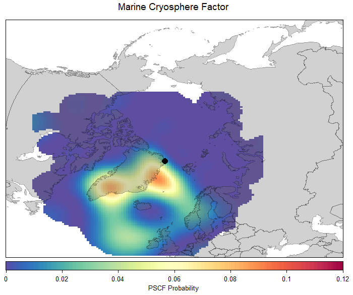
Figure 7PSCF for the marine cryosphere factor and air mass back trajectories arriving at 100 m altitude and extending backward 120 h in time. This plot and analysis method were produced in R and R Studio (R Foundation for Statistical Computing, Vienna, Austria, and R Studio Inc, MA, USA) and the openair suite of analysis tools (Carslaw and Ropkins, 2012).
The spatial origin of the marine cryosphere factor was investigated via a PSCF calculated with the R package openair (Carslaw and Ropkins, 2012). Figure 7 displays the PSCF for air masses arriving every hour during the measurement campaign, which provides increased statistical robustness to the results over calculating a PSCF just for the summer period. From Fig. 7, two areas with a relatively higher probability of being a source region for the marine cryosphere factor can be discerned: the coasts around southeastern and northeastern Greenland. This analysis is supported by the CPF for the marine cryosphere factor (Fig. S8b in the Supplement), which shows the dominant wind direction for this factor to be the south and south-southeast. Lee et al. (2020) used monthly chlorophyll a derived from the MODIS satellite to demonstrate that the coast around northeastern Greenland contains high chlorophyll a concentrations during June, which is supported by previous studies (Degerlund and Eilertsen, 2010; Galí and Simó, 2010). Lee et al. (2020) also used a PSCF to determine this area to be the source regions for total particle number concentrations in the nucleation size range (3–25 nm). This area has been demonstrated to be a source region for MSA during the summer months (Heintzenberg et al., 2017). Thus, we propose the biologically active coasts around eastern Greenland to be the source region for the marine cryosphere factor.
The properties of the marine cryosphere factor (composition, temporal variation, and spatial origins) helps confirm the work of previous studies in the High Arctic. We propose this factor (although not necessarily these exact species) as responsible for the biogenic precursor emissions of particles observed in other studies (Nguyen et al., 2016; Burkart et al., 2017; Dall'Osto et al., 2017, 2018a, b, 2019; Freud et al., 2017; Nielsen et al., 2019). For example, Nguyen et al. (2016) identified the area southeast of Villum as having a high probability of observing an NPF event when air masses originate from this sector. One of the source areas identified in Fig. 7 is southeast of Villum, and a CPF analysis indicated high contributions of the marine cryosphere factor were observed when the wind direction was south of Villum (Fig. S8b in the Supplement). While the species identified using this analytical technique might not be responsible for particle formation and growth, other high molecular weight compounds originating from the same sources could well be. Therefore, this factor has important climatic implications, as sea ice and snowmelt are expected to start earlier due to warming temperatures. Increased contributions from this factor can be expected, which will alter the CCN budget and occurrence in the summer and thus alter the radiative balance.
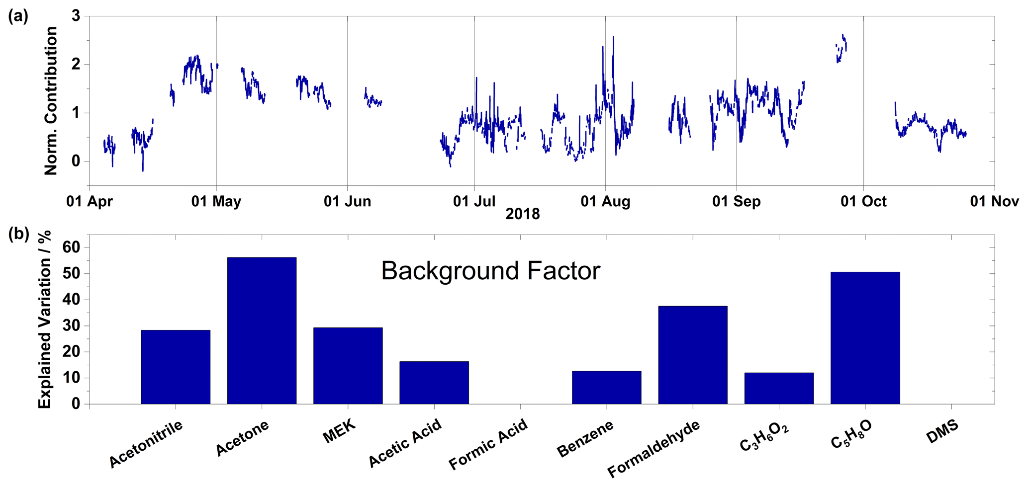
Figure 8(a) Time series of normalized contributions and (b) species profile for the background factor. Factor contributions are normalized to give a mean contribution of unity.
3.3.3 Background factor
The background factor explains the majority (> 50 %) of the variation of acetone and C5H8O as well as 37 % of formaldehyde (Fig. 8a). It explains approximately 30 % of the variation of acetonitrile and MEK, followed by minor (< 20 %) variations of acetic acid, benzene, and C3H6O2. C3H6O2 may in this case result from all three of the isomers: propionic acid, methyl acetate, and hydroxyacetone. Acetone and formaldehyde are known to have photochemical oxidation of precursor compounds in the atmosphere as an important source. The chemical profile of this factor does not point to a specific, known source (Fig. 8b). Its contributions start increasing in the middle of April, reach a maximum by the end of the month, then decrease until the summer period (Fig. 8a). During the autumn, contribution levels are similar to the summer period; however, the temporal pattern is quite similar to the one observed for the biomass burning factor. The temporal correlations of the background factor to the marine cryosphere and biomass burning factor during their respective periods of peak contributions indicate this factor does not arise from one identifiable source but rather from a myriad of sources, hence the assignment as a background factor. The species profile for the background factor corresponds to mixing ratios of 0.355 ppbv for acetone, 0.090 ppbv for formaldehyde, and less than 0.050 ppbv for all other compounds. These mixing ratios can be interpreted as the background mixing ratios for these compounds in the High Arctic.
The background factor has its highest period of mean contributions during the spring, when solar intensity increases but before the emissions related to open sea or melting snow become relevant. This factor likely represents a source of VOCs caused by the increasing rate of photochemical oxidation of labile organic carbon naturally present in the air and on surfaces. Photo-oxidation of alkanes present in the air and deposited during the winter is a possible source of labile organic carbon (Boudries et al., 2002; Guimbaud et al., 2002; Gao et al., 2012). For example, acetone (a major component of the background factor) is primarily formed from reactions of OH and Cl with propane, isobutane, and pentane (Hornbrook et al., 2016). This slow decrease during the spring could be due to the decreasing supply of labile organic carbon in the snowpack. The weak diurnal pattern of this factor in the summer (Fig. 6) could be due to increased available organic matter for oxidation from the open ocean and melting snowpack. Further measurements, especially during the polar night-to-day transition, are required to test this hypothesis.
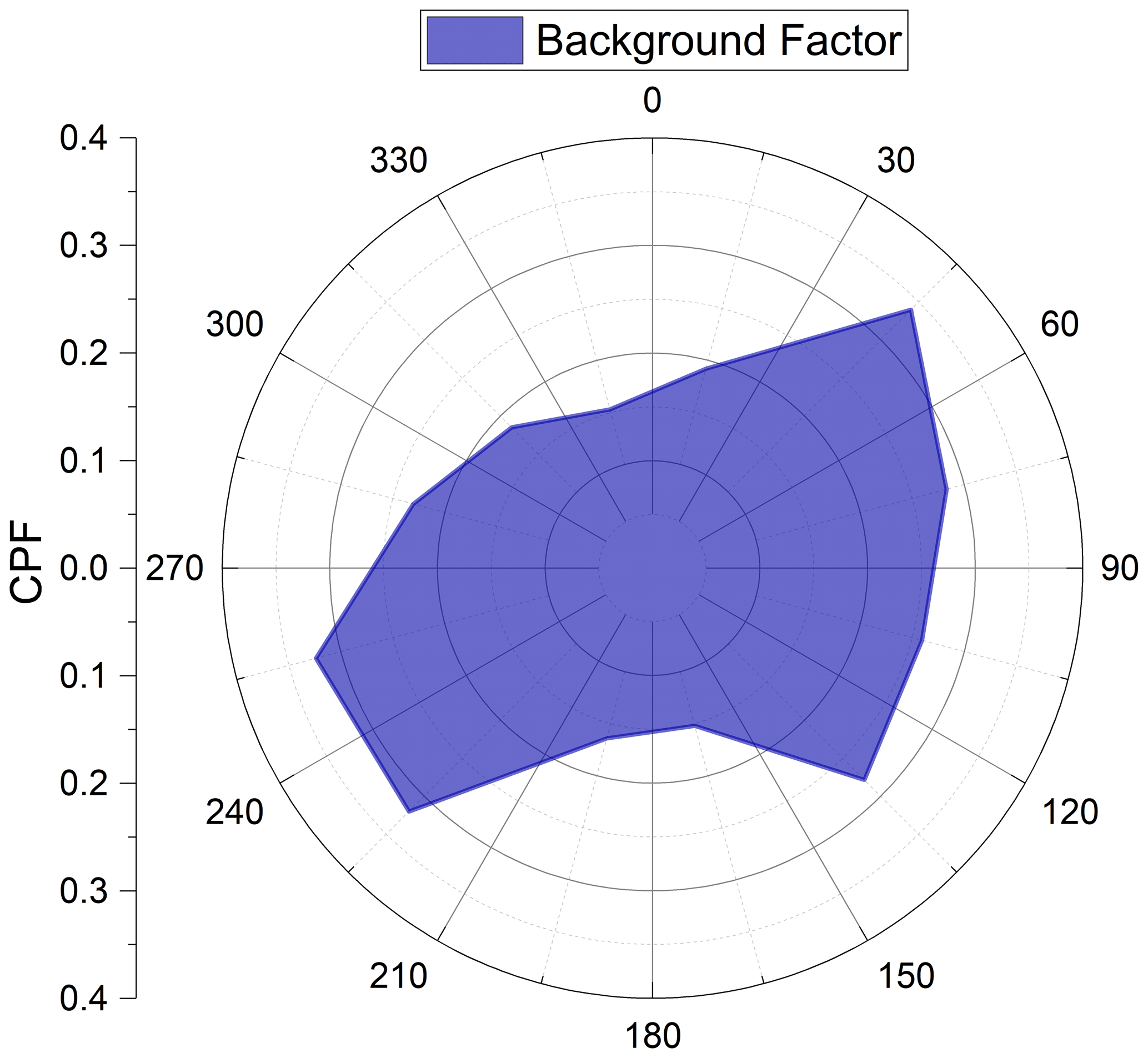
Figure 9Conditional probability function for the background factor from the PMF analysis. CPF was calculated as described in Sect. 2.3.
Given the lack of a peak period for contributions from this factor, we were unable to locate the source regions of this factor through air mass back trajectory analysis. Therefore, local wind direction and normalized contributions for this factor were used to create a conditional probability function (see Sect. 2.3). During the spring and autumn, the dominant wind direction at Villum is from the southwest, while during the summer it is from the east (Nguyen et al., 2016). The CPF can give information regarding the directional dependence of a factor or compound. Figure 9 shows the CPF for the background factor. There is a lack of directional dependence for this factor, indicating this factor does not arise from one specific source area but is rather spatially ubiquitous.
The background factor likely represents natural processes occurring in the Arctic. This factor can serve as a baseline for comparison with future VOC measurements and source apportionment analysis. These comparisons can help expound upon the effects of climate change on the natural processes occurring in this pristine and sensitive region. This, however, requires more long-term VOC measurements, especially across all seasons.
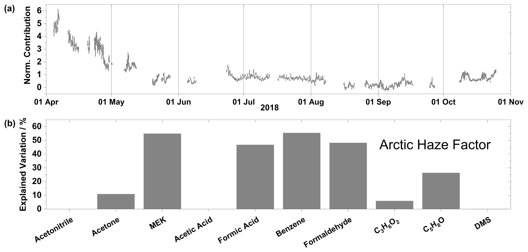
Figure 10(a) Time series of normalized contributions and (b) species profile for the Arctic haze factor. Factor contributions are normalized to give a mean contribution of unity.
3.3.4 Arctic haze factor
The Arctic haze factor exhibits high contributions at the beginning of April and it rapidly decreases until the middle of May, when it remains low and stable for the remaining of the measurement campaign (Fig. 10a). This factor accounts for 56 % of the variation of benzene and zero percent of acetonitrile, which suggests fossil fuel combustion processes as the source of this factor (Liu et al., 2008; Singh et al., 2003) (Fig. 10b). Interestingly, the other species apportioned to this factor with significant contributions, i.e., MEK, formic acid, formaldehyde, and C5H8O (Fig. 10b) are all oxygenated compounds that exhibit decreasing patterns in the spring as well as diurnal variation in the summer (Fig. 2). Much like for the background factor, the source of these OVOCs is the oxidation of labile organic carbon transported from the midlatitudes.
The high levels of anthropogenic pollutants transported to the High Arctic during this period give the well-known “Arctic haze” phenomenon (Barrie et al., 1981). The decrease in mixing ratio during the spring is characteristic of the seasonality for long-range transport for this region (Willis et al., 2018). The mixing ratio of compounds emitted from sources outside the polar dome is drastically reduced in the summer (Klonecki et al., 2003). Also, the faster oxidation rates due to higher OH radical concentrations, as well as increased wet scavenging during transport in summer, will reduce VOC and BC mixing ratios (Browse et al., 2012). Gautrois et al. (2003) reported benzene mixing ratios for 7 years at Alert, NU, and found an annual variation similar to observations for the Arctic haze factor in this study. The enhanced levels of BC (not shown) during this period (and lack thereof during summer and autumn) support the assignment of this factor to anthropogenic combustion sources.
The Arctic haze factor presented in this study can be compared to other Arctic haze factors previously found using factor analysis or clustering of either aerosol composition or PNSD data. It is worth noting that the Arctic haze factor from this study is only for spring, while the other studies present data from the winter and spring, therefore any comparisons we make are from our spring Arctic haze factor to other haze factors during winter and spring. While this is not a perfect comparison, it is one worth making, as Arctic haze is the main source of anthropogenic pollution in the Arctic. Lange et al. (2018) used k-means clustering of aerosol size distribution to classify the accumulation mode aerosol population from Villum. The authors found three accumulation mode clusters; the one they named “Haze” occurred predominately in the winter/spring and was largely absent in the summer. The Haze cluster contained the largest amounts of refractory BC, sulfate, and organics as well as the highest concentrations of CCN. Extending this analysis into the chemical composition of aerosols, Nielsen et al. (2019) utilized PMF to find three factors. The factor deemed “Arctic haze organic aerosol” was closely correlated with sulfate and temporally followed the pattern exhibited by the Haze cluster from Lange et al. (2018) and the Arctic haze factor (this study), due to the contraction of the polar dome in spring. These similar factors/clusters resolved from different data sources (PNSD, aerosol chemical composition, and VOCs) and different statistical methods (k-means and PMF) highlight the extent to how anthropogenic pollution can influence the characteristics of the High Arctic atmosphere. Given recent trends in emission reductions across Europe and Eurasia, these factors/clusters are expected to decrease in magnitude, although the extent and occurrence of this anthropogenic pollution will ultimately be governed by several factors including transport patterns, precipitation patterns, and expansion of anthropogenic pollution sources within the Arctic Circle (resource extraction and shipping) (Law et al., 2017).
VOC mixing ratios were measured during April–October 2018 at the High Arctic Villum Research Station located at Station Nord in northeast Greenland. We identified 10 compounds by PTR-ToF-MS and provided time series of VOCs in the High Arctic covering several months. Generally, the mixing ratios observed in the present study are in accordance with other VOC measurements carried out in Arctic locations. We apportioned sources of these VOCs using PMF, finding four factors: biomass burning, marine cryosphere, background, and Arctic haze. The biomass burning factor exhibited maxima during the autumn and the chemical profile was dominated by acetonitrile with contributions from benzene. Interestingly, BC did not show enhancements during the peak of the biomass burning factor, which we show is due to washout during transport. The marine cryosphere factor was described by carboxylic acids (formic and acetic acid and possibly propionic acid from C3H6O2) and DMS. This factor displayed maxima in the summer during periods of snow and sea ice melt. A PSCF analysis yielded the coasts of southeastern and northeastern Greenland as source regions for this factor. The background factor showed maxima in the spring and autumn, and minima during the summer. While acetone was the dominating species in this factor, the chemical profile did not resemble any known processes or sources. Oxidation of labile organic carbon is proposed as the source of the OVOCs present in this factor. The Arctic haze factor peaked in April, decreased until mid-May, and was absent during the summer. This factor was driven by benzene as well as OVOCs. The source of OVOCs present in this factor is postulated to be the oxidation of precursor emissions during transport from the midlatitudes to the Arctic.
This study has several important results that have implications for the Arctic climate. Recent studies have highlighted the importance of natural emissions to aerosol formation and their contribution to CCN concentrations in the summer (Leaitch et al., 2016; Lange et al., 2019; Nielsen et al., 2019). The marine cryosphere factor presents an important source of condensable vapors necessary for this formation and growth to CCN sizes. Due to increasing temperatures in the Arctic, the snowpack and sea ice are expected to experience increased melting in the coming years, which could increase the flux of DMS and carboxylic acids from the surface to the atmosphere. With the onset of the melt season in the Arctic expected to begin earlier in the future, we also expect that the timing of this onset can affect NPF events and their subsequent growth as well as ozone photochemistry. While biomass burning is expected to increase in the future, the year-to-year variability is still highly uncertain. The biomass burning factor was characterized by acetonitrile, benzene, and correlated temporally with ozone. Due to washout during transport, there were no enhancements in BC during the peak of the biomass burning factor. The interannual variability of biomass burning events and meteorological conditions can, therefore, have a substantial impact on atmospheric pollution levels at ground level.
While this research provides valuable insight into the atmospheric chemistry and sources of VOCs in the High Arctic, future work is still needed. While calculated mixing ratios using a kinetic quantification are reliable, they are inherently uncertain; therefore, external calibration with gas-phase standards would greatly improve the accuracy and reduce the analytical uncertainty. This work presents a multiseason time series of VOC mixing ratios; however, these measurements are only during polar day. A full seasonal cycle including polar night, dark-to-light transition periods, and polar day would help elucidate the importance of transport of anthropogenic emissions in the absence of photochemical reactions. This work expounds on the understanding of the atmospheric chemistry and sources of VOCs in the High Arctic; however, future research is needed to fully understand the biogeochemical feedback mechanisms and their implications for a changing Arctic.
All data used in this publication are available at https://doi.org/10.5281/zenodo.4299817 (Pernov et al., 2020) or by request to the corresponding authors Jakob B. Pernov (jbp@envs.au.dk) and Rossana Bossi (rbo@envs.au.dk).
The supplement related to this article is available online at: https://doi.org/10.5194/acp-21-2895-2021-supplement.
JBP, RB, and RH collected the measurements. JBP and RB processed the data. JBP, JLH, RB, and TL analyzed the data. JBP, JKN, and TL performed the PMF analysis. JBP and JLH wrote the manuscript. HSK provided the initial project funding and idea for VOC measurements at Villum. All coauthors proofread and commented on the manuscript.
The authors declare that they have no conflict of interest.
The Villum Foundation is gratefully acknowledged for financing the establishment of the Villum Research Station and the instrumentation used in this study (PTR-ToF-MS). Thanks to the Royal Danish Air Force and the Arctic Command for providing logistic support to the project. Christel Christoffersen, Bjarne Jensen, and Keld Mortensen are gratefully acknowledged for their technical support. We acknowledge the use of data from the NASA FIRMS application (https://firms.modaps.eosdis.nasa.gov/, last access: 14 November 2020) operated by the NASA/Goddard Space Flight Center Earth Science Data and Information System (ESDIS) project and NASA's Earth Science Data and Information System (ESDIS) with funding provided by NASA Headquarters. We thank NOAA for use of the HYSPLIT model. We thank David Carslaw for developing the openair function. We acknowledge Chad Greene for the use of MATLAB functions (Greene et al., 2017). We acknowledge Francesco Canonaco for helpful discussions on the PMF analysis as well as Ksenia Tabakova and Paul Glantz for help with HYSPLIT and MATLAB.
This research has been financially supported by the Danish Environmental Protection Agency and the Danish Energy Agency, with means from MIKA/DANCEA funds for environmental support to the Arctic region (project nos. Danish EPA: MST-113-00-140; Ministry of Climate, Energy, and Utilities: 2018-3767) and ERA-PLANET (The European Network for observing our changing Planet) projects, as well as by iGOSP, iCUPE, and finally by the Graduate School of Science and Technology, Aarhus University.
This paper was edited by Kyung-Eun Min and reviewed by two anonymous referees.
AMAP: AMAP Assessment 2015: Black carbon and ozone as Arctic climate forcers, Arctic Monitoring and Assessment Programme (AMAP), Oslo, Norway, 116, 2015.
Anderson, C. H., Dibb, J. E., Griffin, R. J., Hagler, G. S. W., and Bergin, M. H.: Atmospheric water-soluble organic carbon measurements at Summit, Greenland, Atmos. Environ., 42, 5612–5621, https://doi.org/10.1016/j.atmosenv.2008.03.006, 2008.
Andreae, M. O.: Emission of trace gases and aerosols from biomass burning – an updated assessment, Atmos. Chem. Phys., 19, 8523–8546, https://doi.org/10.5194/acp-19-8523-2019, 2019.
Arnold, S. R., Emmons, L. K., Monks, S. A., Law, K. S., Ridley, D. A., Turquety, S., Tilmes, S., Thomas, J. L., Bouarar, I., Flemming, J., Huijnen, V., Mao, J., Duncan, B. N., Steenrod, S., Yoshida, Y., Langner, J., and Long, Y.: Biomass burning influence on high-latitude tropospheric ozone and reactive nitrogen in summer 2008: a multi-model analysis based on POLMIP simulations, Atmos. Chem. Phys., 15, 6047–6068, https://doi.org/10.5194/acp-15-6047-2015, 2015.
Barret, M., Domine, F., Houdier, S., Gallet, J. C., Weibring, P., Walega, J., Fried, A., and Richter, D.: Formaldehyde in the Alaskan Arctic snowpack: Partitioning and physical processes involved in air-snow exchanges, J. Geophys. Res.-Atmos., 116, D00R03, https://doi.org/10.1029/2011jd016038, 2011.
Barrie, L. A., Hoff, R. M., and Daggupaty, S. M.: The influence of mid-latitudinal pollution sources on haze in the Canadian arctic, Atmos. Environ., 15, 1407–1419, https://doi.org/10.1016/0004-6981(81)90347-4, 1981.
Bell, T. G., De Bruyn, W., Miller, S. D., Ward, B., Christensen, K. H., and Saltzman, E. S.: Air–sea dimethylsulfide (DMS) gas transfer in the North Atlantic: evidence for limited interfacial gas exchange at high wind speed, Atmos. Chem. Phys., 13, 11073–11087, https://doi.org/10.5194/acp-13-11073-2013, 2013.
Bi, H. B., Zhang, J. L., Wang, Y. H., Zhang, Z. H., Zhang, Y., Fu, M., Huang, H. J., and Xu, X. L.: Arctic Sea Ice Volume Changes in Terms of Age as Revealed From Satellite Observations, IEEE J. Sel. Top. Appl., 11, 2223–2237, https://doi.org/10.1109/jstars.2018.2823735, 2018.
Boe, J. L., Hall, A., and Qu, X.: September sea-ice cover in the Arctic Ocean projected to vanish by 2100, Nat. Geosci., 2, 341–343, https://doi.org/10.1038/ngeo467, 2009.
Boudries, H., Bottenheim, J. W., Guimbaud, C., Grannas, A. M., Shepson, P. B., Houdier, S., Perrier, S., and Dominé, F.: Distribution and trends of oxygenated hydrocarbons in the high Arctic derived from measurements in the atmospheric boundary layer and interstitial snow air during the ALERT2000 field campaign, Atmos. Environ., 36, 2573–2583, https://doi.org/10.1016/S1352-2310(02)00122-X, 2002.
Brewer, J. F., Fischer, E. V., Commane, R., Wofsy, S. C., Daube, B. C., Apel, E. C., Hills, A. J., Hornbrook, R. S., Barletta, B., Meinardi, S., Blake, D. R., Ray, E. A., and Ravishankara, A. R.: Evidence for an Oceanic Source of Methyl Ethyl Ketone to the Atmosphere, Geophys. Res. Lett., 47, e2019GL086045, https://doi.org/10.1029/2019GL086045, 2020.
Brown, S. G., Eberly, S., Paatero, P., and Norris, G. A.: Methods for estimating uncertainty in PMF solutions: Examples with ambient air and water quality data and guidance on reporting PMF results, Sci. Total Environ., 518–519, 626–635, https://doi.org/10.1016/j.scitotenv.2015.01.022, 2015.
Browse, J., Carslaw, K. S., Arnold, S. R., Pringle, K., and Boucher, O.: The scavenging processes controlling the seasonal cycle in Arctic sulphate and black carbon aerosol, Atmos. Chem. Phys., 12, 6775–6798, https://doi.org/10.5194/acp-12-6775-2012, 2012.
Bruggemann, M., Hayeck, N., and George, C.: Interfacial photochemistry at the ocean surface is a global source of organic vapors and aerosols, Nat. Commun., 9, 2101, https://doi.org/10.1038/s41467-018-04528-7, 2018.
Burkart, J., Hodshire, A. L., Mungall, E. L., Pierce, J. R., Collins, D. B., Ladino, L. A., Lee, A. K. Y., Irish, V., Wentzell, J. J. B., Liggio, J., Papakyriakou, T., Murphy, J., and Abbatt, J.: Organic Condensation and Particle Growth to CCN Sizes in the Summertime Marine Arctic Is Driven by Materials More Semivolatile Than at Continental Sites, Geophys. Res. Lett., 44, 10725–10734, https://doi.org/10.1002/2017gl075671, 2017.
Carslaw, D. C. and Ropkins, K.: openair – An R package for air quality data analysis, Environ. Modell. Softw., 27–28, 52–61, https://doi.org/10.1016/j.envsoft.2011.09.008, 2012.
Cavalieri, D. J., Parkinson, C. L., Gloersen, P., and Zwally, H. J.: Sea Ice Concentrations from Nimbus-7 SMMR and DMSP SSM/I-SSMIS Passive Microwave Data, Version 1, NASA National Snow and Ice Data Center Distributed Active Archive Center, Boulder, Colorado USA, https://doi.org/10.5067/8GQ8LZQVL0VL, 1996.
Chiu, R., Tinel, L., Gonzalez, L., Ciuraru, R., Bernard, F., George, C., and Volkamer, R.: UV photochemistry of carboxylic acids at the air–sea boundary: A relevant source of glyoxal and other oxygenated VOC in the marine atmosphere, Geophys. Res. Lett., 44, 1079–1087, https://doi.org/10.1002/2016gl071240, 2017.
Dai, A. G., Luo, D. H., Song, M. R., and Liu, J. P.: Arctic amplification is caused by sea-ice loss under increasing CO2, Nat. Commun., 10, 121, https://doi.org/10.1038/s41467-018-07954-9, 2019.
Dall'Osto, M., Beddows, D. C. S., Tunved, P., Krejci, R., Ström, J., Hansson, H. C., Yoon, Y. J., Park, K.-T., Becagli, S., Udisti, R., Onasch, T., O'Dowd, C. D., Simó, R., and Harrison, R. M.: Arctic sea ice melt leads to atmospheric new particle formation, Sci. Rep.-UK, 7, 3318, https://doi.org/10.1038/s41598-017-03328-1, 2017.
Dall'Osto, M., Geels, C., Beddows, D. C. S., Boertmann, D., Lange, R., Nojgaard, J. K., Harrison, R. M., Simo, R., Skov, H., and Massling, A.: Regions of open water and melting sea ice drive new particle formation in North East Greenland, Sci. Rep.-UK, 8, 6109, https://doi.org/10.1038/s41598-018-24426-8, 2018a.
Dall'Osto, M., Simo, R., Harrison, R. M., Beddows, D. C. S., Saiz-Lopez, A., Lange, R., Skov, H., Nojgaard, J. K., Nielsen, I. E., and Massling, A.: Abiotic and biotic sources influencing spring new particle formation in North East Greenland, Atmos. Environ., 190, 126–134, https://doi.org/10.1016/j.atmosenv.2018.07.019, 2018b.
Dall'Osto, M., Beddows, D. C. S., Tunved, P., Harrison, R. M., Lupi, A., Vitale, V., Becagli, S., Traversi, R., Park, K.-T., Yoon, Y. J., Massling, A., Skov, H., Lange, R., Strom, J., and Krejci, R.: Simultaneous measurements of aerosol size distributions at three sites in the European high Arctic, Atmos. Chem. Phys., 19, 7377–7395, https://doi.org/10.5194/acp-19-7377-2019, 2019.
de Gouw, J. and Warneke, C.: Measurements of volatile organic compounds in the Earth's atmosphere using proton-transfer-reaction mass spectrometry, Mass Spectrom. Rev., 26, 223–257, https://doi.org/10.1002/mas.20119, 2007.
de Gouw, J. A., Warneke, C., Parrish, D. D., Holloway, J. S., Trainer, M., and Fehsenfeld, F. C.: Emission sources and ocean uptake of acetonitrile (CH3CN) in the atmosphere, J. Geophys. Res.-Atmos., 108, 4329, https://doi.org/10.1029/2002jd002897, 2003.
Degerlund, M. and Eilertsen, H. C.: Main Species Characteristics of Phytoplankton Spring Blooms in NE Atlantic and Arctic Waters (68–80∘ N), Estuar. Coast., 33, 242–269, https://doi.org/10.1007/s12237-009-9167-7, 2010.
Dibb, J. E. and Arsenault, M.: Shouldn't snowpacks be sources of monocarboxylic acids?, Atmos. Environ., 36, 2513–2522, https://doi.org/10.1016/s1352-2310(02)00131-0, 2002.
Draxler, R. R. and Hess, G. D.: An overview of the HYSPLIT_4 modelling system for trajectories, dispersion and deposition, Aust. Meteorol. Mag., 47, 295–308, 1998.
Freud, E., Krejci, R., Tunved, P., Leaitch, R., Nguyen, Q. T., Massling, A., Skov, H., and Barrie, L.: Pan-Arctic aerosol number size distributions: seasonality and transport patterns, Atmos. Chem. Phys., 17, 8101–8128, https://doi.org/10.5194/acp-17-8101-2017, 2017.
Galí, M. and Simó, R.: Occurrence and cycling of dimethylated sulfur compounds in the Arctic during summer receding of the ice edge, Mar. Chem., 122, 105–117, https://doi.org/10.1016/j.marchem.2010.07.003, 2010.
Gao, S. S., Sjostedt, S. J., Sharma, S., Hall, S. R., Ullmann, K., and Abbatt, J. P. D.: PTR-MS observations of photo-enhanced VOC release from Arctic and midlatitude snow, J. Geophys. Res.-Atmos., 117, D00R17, https://doi.org/10.1029/2011JD017152, 2012.
Gautrois, M., Brauers, T., Koppmann, R., Rohrer, F., Stein, O., and Rudolph, J.: Seasonal variability and trends of volatile organic compounds in the lower polar troposphere, J. Geophys. Res.-Atmos., 108, 4393, https://doi.org/10.1029/2002JD002765, 2003.
Glasius, M., Boel, C., Bruun, N., Easa, L. M., Hornung, P., Klausen, H. S., Klitgaard, K. C., Lindeskov, C., Moller, C. K., Nissen, H., Petersen, A. P. F., Kleefeld, S., Boaretto, E., Hansen, T. S., Heinemeier, J., and Lohse, C.: Relative contribution of biogenic and anthropogenic sources to formic and acetic acids in the atmospheric boundary layer, J. Geophys. Res.-Atmos., 106, 7415–7426, https://doi.org/10.1029/2000jd900676, 2001.
Grannas, A. M., Shepson, P. B., Guimbaud, C., Sumner, A. L., Albert, M., Simpson, W., Domine, F., Boudries, H., Bottenheim, J., Beine, H. J., Honrath, R., and Zhou, X. L.: A study of photochemical and physical processes affecting carbonyl compounds in the Arctic atmospheric boundary layer, Atmos. Environ., 36, 2733–2742, https://doi.org/10.1016/s1352-2310(02)00134-6, 2002.
Grannas, A. M., Shepson, P. B., and Filley, T. R.: Photochemistry and nature of organic matter in Arctic and Antarctic snow, Global Biogeochem. Cy., 18, GB1006, https://doi.org/10.1029/2003gb002133, 2004.
Greene, C. A.: Arctic Sea ice: available at: https://www.mathworks.com/matlabcentral/fileexchange/56923-arctic-sea-ice, last access: 26 January 2020.
Greene, C. A., Gwyther, D. E., and Blankenship, D. D.: Antarctic Mapping Tools for MATLAB, Comput. Geosci., 104, 151–157, https://doi.org/10.1016/j.cageo.2016.08.003, 2017.
Guimbaud, C., Grannas, A. M., Shepson, P. B., Fuentes, J. D., Boudries, H., Bottenheim, J. W., Domine, F., Houdier, S., Perrier, S., Biesenthal, T. B., and Splawn, B. G.: Snowpack processing of acetaldehyde and acetone in the Arctic atmospheric boundary layer, Atmos. Environ., 36, 2743–2752, https://doi.org/10.1016/s1352-2310(02)00107-3, 2002.
Hamm, S. and Warneck, P.: The interhemispheric distribution and the budget of acetonitrile in the troposphere, J. Geophys. Res.-Atmos., 95, 20593–20606, https://doi.org/10.1029/JD095iD12p20593, 1990.
Hamm, S., Hahn, J., Helas, G., and Warneck, P.: Acetonitrile in the troposphere: Residence time due to rainout and uptake by the ocean, Geophys. Res. Lett., 11, 1207–1210, https://doi.org/10.1029/GL011i012p01207, 1984.
Harrigan, D. L., Fuelberg, H. E., Simpson, I. J., Blake, D. R., Carmichael, G. R., and Diskin, G. S.: Anthropogenic emissions during Arctas-A: mean transport characteristics and regional case studies, Atmos. Chem. Phys., 11, 8677–8701, https://doi.org/10.5194/acp-11-8677-2011, 2011.
Haywood, J. and Boucher, O.: Estimates of the direct and indirect radiative forcing due to tropospheric aerosols: A review, Rev. Geophys., 38, 513–543, https://doi.org/10.1029/1999rg000078, 2000.
Heintzenberg, J., Tunved, P., Galí, M., and Leck, C.: New particle formation in the Svalbard region 2006–2015, Atmos. Chem. Phys., 17, 6153–6175, https://doi.org/10.5194/acp-17-6153-2017, 2017.
Hirdman, D., Aspmo, K., Burkhart, J. F., Eckhardt, S., Sodemann, H., and Stohl, A.: Transport of mercury in the Arctic atmosphere: Evidence for a spring-time net sink and summer-time source, Geophys. Res. Lett., 36, L12814, https://doi.org/10.1029/2009gl038345, 2009.
Holzinger, R., Jordan, A., Hansel, A., and Lindinger, W.: Automobile emissions of acetonitrile: Assessment of its contribution to the global source, J. Atmos. Chem., 38, 187–193, https://doi.org/10.1023/a:1006435723375, 2001.
Holzinger, R., Acton, W. J. F., Bloss, W. J., Breitenlechner, M., Crilley, L. R., Dusanter, S., Gonin, M., Gros, V., Keutsch, F. N., Kiendler-Scharr, A., Kramer, L. J., Krechmer, J. E., Languille, B., Locoge, N., Lopez-Hilfiker, F., Materić, D., Moreno, S., Nemitz, E., Quéléver, L. L. J., Sarda Esteve, R., Sauvage, S., Schallhart, S., Sommariva, R., Tillmann, R., Wedel, S., Worton, D. R., Xu, K., and Zaytsev, A.: Validity and limitations of simple reaction kinetics to calculate concentrations of organic compounds from ion counts in PTR-MS, Atmos. Meas. Tech., 12, 6193–6208, https://doi.org/10.5194/amt-12-6193-2019, 2019.
Hopke, P. K.: Review of receptor modeling methods for source apportionment, J. Air Waste Manage., 66, 237–259, https://doi.org/10.1080/10962247.2016.1140693, 2016.
Hornbrook, R. S., Hills, A. J., Riemer, D. D., Abdelhamid, A., Flocke, F. M., Hall, S. R., Huey, L. G., Knapp, D. J., Liao, J., Mauldin, R. L., Montzka, D. D., Orlando, J. J., Shepson, P. B., Sive, B., Staebler, R. M., Tanner, D. J., Thompson, C. R., Turnipseed, A., Ullmann, K., Weinheimer, A. J., and Apel, E. C.: Arctic springtime observations of volatile organic compounds during the OASIS-2009 campaign, J. Geophys. Res.-Atmos., 121, 9789–9813, https://doi.org/10.1002/2015jd024360, 2016.
Jacob, D. J., Field, B. D., Jin, E. M., Bey, I., Li, Q., Logan, J. A., Yantosca, R. M., and Singh, H. B.: Atmospheric budget of acetone, J. Geophys. Res.-Atmos., 107, ACH 5-1–ACH 5-17, https://doi.org/10.1029/2001JD000694, 2002.
Karl, T., Guenther, A., Turnipseed, A., Tyndall, G., Artaxo, P., and Martin, S.: Rapid formation of isoprene photo-oxidation products observed in Amazonia, Atmos. Chem. Phys., 9, 7753–7767, https://doi.org/10.5194/acp-9-7753-2009, 2009.
Kecorius, S., Vogl, T., Paasonen, P., Lampilahti, J., Rothenberg, D., Wex, H., Zeppenfeld, S., van Pinxteren, M., Hartmann, M., Henning, S., Gong, X., Welti, A., Kulmala, M., Stratmann, F., Herrmann, H., and Wiedensohler, A.: New particle formation and its effect on cloud condensation nuclei abundance in the summer Arctic: a case study in the Fram Strait and Barents Sea, Atmos. Chem. Phys., 19, 14339–14364, https://doi.org/10.5194/acp-19-14339-2019, 2019.
Kiene, R. P., Linn, L. J., and Bruton, J. A.: New and important roles for DMSP in marine microbial communities, J. Sea Res., 43, 209–224, https://doi.org/10.1016/s1385-1101(00)00023-x, 2000.
Klonecki, A., Hess, P., Emmons, L., Smith, L., Orlando, J., and Blake, D.: Seasonal changes in the transport of pollutants into the Arctic troposphere-model study, J. Geophys. Res.-Atmos., 108, 8367, https://doi.org/10.1029/2002jd002199, 2003.
Kos, G., Kanthasami, V., Adechina, N., and Ariya, P. A.: Volatile organic compounds in Arctic snow: concentrations and implications for atmospheric processes, Environ. Sci.-Proc. Imp., 16, 2592–2603, https://doi.org/10.1039/c4em00410h, 2014.
Lange, R., Dall'Osto, M., Skov, H., Nojgaard, J. K., Nielsen, I. E., Beddows, D. C. S., Simob, R., Harrison, R. M., and Massling, A.: Characterization of distinct Arctic aerosol accumulation modes and their sources, Atmos. Environ., 183, 1–10, https://doi.org/10.1016/j.atmosenv.2018.03.060, 2018.
Lange, R., Dall'Osto, M., Wex, H., Skov, H., and Massling, A.: Large Summer Contribution of Organic Biogenic Aerosols to Arctic Cloud Condensation Nuclei, Geophys. Res. Lett., 46, 11500–11509, https://doi.org/10.1029/2019gl084142, 2019.
Languille, B., Gros, V., Petit, J.-E., Honoré, C., Baudic, A., Perrussel, O., Foret, G., Michoud, V., Truong, F., Bonnaire, N., Sarda-Estève, R., Delmotte, M., Feron, A., Maisonneuve, F., Gaimoz, C., Formenti, P., Kotthaus, S., Haeffelin, M., and Favez, O.: Wood burning: A major source of Volatile Organic Compounds during wintertime in the Paris region, Sci. Total Environ., 711, 135055, https://doi.org/10.1016/j.scitotenv.2019.135055, 2020.
Lavoue, D., Liousse, C., Cachier, H., Stocks, B. J., and Goldammer, J. G.: Modeling of carbonaceous particles emitted by boreal and temperate wildfires at northern latitudes, J. Geophys. Res.-Atmos., 105, 26871–26890, https://doi.org/10.1029/2000jd900180, 2000.
Law, K. S., Roiger, A., Thomas, J. L., Marelle, L., Raut, J. C., Dalsoren, S., Fuglestvedt, J., Tuccella, P., Weinzierl, B., and Schlager, H.: Local Arctic air pollution: Sources and impacts, Ambio, 46, 453–463, https://doi.org/10.1007/s13280-017-0962-2, 2017.
Leaitch, W. R., Korolev, A., Aliabadi, A. A., Burkart, J., Willis, M. D., Abbatt, J. P. D., Bozem, H., Hoor, P., Köllner, F., Schneider, J., Herber, A., Konrad, C., and Brauner, R.: Effects of 20–100 nm particles on liquid clouds in the clean summertime Arctic, Atmos. Chem. Phys., 16, 11107–11124, https://doi.org/10.5194/acp-16-11107-2016, 2016.
Lee, B., Hwangbo, Y., and Soo Lee, D.: Determination of Low Molecular Weight Monocarboxylic Acid Gases in the Atmosphere by Parallel Plate Diffusion Scrubber-Ion Chromatography, J. Chromatogr. Sci., 47, 516–522, https://doi.org/10.1093/chromsci/47.7.516, 2009.
Lee, H., Lee, K., Lunder, C. R., Krejci, R., Aas, W., Park, J., Park, K.-T., Lee, B. Y., Yoon, Y. J., and Park, K.: Atmospheric new particle formation characteristics in the Arctic as measured at Mount Zeppelin, Svalbard, from 2016 to 2018, Atmos. Chem. Phys., 20, 13425–13441, https://doi.org/10.5194/acp-20-13425-2020, 2020.
Levasseur, M.: Impact of Arctic meltdown on the microbial cycling of sulphur, Nat. Geosci., 6, 691–700, https://doi.org/10.1038/ngeo1910, 2013.
Lewis, A. C., Evans, M. J., Hopkins, J. R., Punjabi, S., Read, K. A., Purvis, R. M., Andrews, S. J., Moller, S. J., Carpenter, L. J., Lee, J. D., Rickard, A. R., Palmer, P. I., and Parrington, M.: The influence of biomass burning on the global distribution of selected non-methane organic compounds, Atmos. Chem. Phys., 13, 851–867, https://doi.org/10.5194/acp-13-851-2013, 2013.
Liu, Y., Shao, M., Fu, L., Lu, S., Zeng, L., and Tang, D.: Source profiles of volatile organic compounds (VOCs) measured in China: Part I, Atmos. Environ., 42, 6247–6260, https://doi.org/10.1016/j.atmosenv.2008.01.070, 2008.
Lund, M. T., Samset, B. H., Skeie, R. B., Watson-Parris, D., Katich, J. M., Schwarz, J. P., and Weinzierl, B.: Short Black Carbon lifetime inferred from a global set of aircraft observations, Npj Climate and Atmospheric Science, 1, https://doi.org/10.1038/s41612-018-0040-x, 2018.
Lutsch, E., Strong, K., Jones, D. B. A., Blumenstock, T., Conway, S., Fisher, J. A., Hannigan, J. W., Hase, F., Kasai, Y., Mahieu, E., Makarova, M., Morino, I., Nagahama, T., Notholt, J., Ortega, I., Palm, M., Poberovskii, A. V., Sussmann, R., and Warneke, T.: Detection and attribution of wildfire pollution in the Arctic and northern midlatitudes using a network of Fourier-transform infrared spectrometers and GEOS-Chem, Atmos. Chem. Phys., 20, 12813–12851, https://doi.org/10.5194/acp-20-12813-2020, 2020.
Massling, A., Nielsen, I. E., Kristensen, D., Christensen, J. H., Sørensen, L. L., Jensen, B., Nguyen, Q. T., Nøjgaard, J. K., Glasius, M., and Skov, H.: Atmospheric black carbon and sulfate concentrations in Northeast Greenland, Atmos. Chem. Phys., 15, 9681–9692, https://doi.org/10.5194/acp-15-9681-2015, 2015.
Millet, D. B., Baasandorj, M., Farmer, D. K., Thornton, J. A., Baumann, K., Brophy, P., Chaliyakunnel, S., de Gouw, J. A., Graus, M., Hu, L., Koss, A., Lee, B. H., Lopez-Hilfiker, F. D., Neuman, J. A., Paulot, F., Peischl, J., Pollack, I. B., Ryerson, T. B., Warneke, C., Williams, B. J., and Xu, J.: A large and ubiquitous source of atmospheric formic acid, Atmos. Chem. Phys., 15, 6283–6304, https://doi.org/10.5194/acp-15-6283-2015, 2015.
Mungall, E. L., Abbatt, J. P. D., Wentzell, J. J. B., Lee, A. K. Y., Thomas, J. L., Blais, M., Gosselin, M., Miller, L. A., Papakyriakou, T., Willis, M. D., and Liggio, J.: Microlayer source of oxygenated volatile organic compounds in the summertime marine Arctic boundary layer, P. Natl. Acad. Sci. USA, 114, 6203–6208, https://doi.org/10.1073/pnas.1620571114, 2017.
Mungall, E. L., Abbatt, J. P. D., Wentzell, J. J. B., Wentworth, G. R., Murphy, J. G., Kunkel, D., Gute, E., Tarasick, D. W., Sharma, S., Cox, C. J., Uttal, T., and Liggio, J.: High gas-phase mixing ratios of formic and acetic acid in the High Arctic, Atmos. Chem. Phys., 18, 10237–10254, https://doi.org/10.5194/acp-18-10237-2018, 2018.
Müller, M., Graus, M., Ruuskanen, T. M., Schnitzhofer, R., Bamberger, I., Kaser, L., Titzmann, T., Hörtnagl, L., Wohlfahrt, G., Karl, T., and Hansel, A.: First eddy covariance flux measurements by PTR-TOF, Atmos. Meas. Tech., 3, 387–395, https://doi.org/10.5194/amt-3-387-2010, 2010.
Nguyen, Q. T., Kristensen, T. B., Hansen, A. M. K., Skov, H., Bossi, R., Massling, A., Sørensen, L. L., Bilde, M., Glasius, M., and Nøjgaard, J. K.: Characterization of humic-like substances in Arctic aerosols, J. Geophys. Res.-Atmos., 119, 5011–5027, https://doi.org/10.1002/2013jd020144, 2014.
Nguyen, Q. T., Glasius, M., Sørensen, L. L., Jensen, B., Skov, H., Birmili, W., Wiedensohler, A., Kristensson, A., Nøjgaard, J. K., and Massling, A.: Seasonal variation of atmospheric particle number concentrations, new particle formation and atmospheric oxidation capacity at the high Arctic site Villum Research Station, Station Nord, Atmos. Chem. Phys., 16, 11319–11336, https://doi.org/10.5194/acp-16-11319-2016, 2016.
Nielsen, I. E., Skov, H., Massling, A., Eriksson, A. C., Dall'Osto, M., Junninen, H., Sarnela, N., Lange, R., Collier, S., Zhang, Q., Cappa, C. D., and Nøjgaard, J. K.: Biogenic and anthropogenic sources of aerosols at the High Arctic site Villum Research Station, Atmos. Chem. Phys., 19, 10239–10256, https://doi.org/10.5194/acp-19-10239-2019, 2019.
Paatero, P. and Tapper, U.: Positive matrix factorization: A non-negative factor model with optimal utilization of error estimates of data values, Environmetrics, 5, 111–126, https://doi.org/10.1002/env.3170050203, 1994.
Paatero, P., Eberly, S., Brown, S. G., and Norris, G. A.: Methods for estimating uncertainty in factor analytic solutions, Atmos. Meas. Tech., 7, 781–797, https://doi.org/10.5194/amt-7-781-2014, 2014.
Pagonis, D., Sekimoto, K., and de Gouw, J.: A Library of Proton-Transfer Reactions of H3O+ Ions Used for Trace Gas Detection, J. Am. Soc. Mass Spectr., 30, 1330–1335, https://doi.org/10.1007/s13361-019-02209-3, 2019.
Parrish, D. D., Law, K. S., Staehelin, J., Derwent, R., Cooper, O. R., Tanimoto, H., Volz-Thomas, A., Gilge, S., Scheel, H.-E., Steinbacher, M., and Chan, E.: Long-term changes in lower tropospheric baseline ozone concentrations at northern mid-latitudes, Atmos. Chem. Phys., 12, 11485–11504, https://doi.org/10.5194/acp-12-11485-2012, 2012.
Paulot, F., Wunch, D., Crounse, J. D., Toon, G. C., Millet, D. B., DeCarlo, P. F., Vigouroux, C., Deutscher, N. M., González Abad, G., Notholt, J., Warneke, T., Hannigan, J. W., Warneke, C., de Gouw, J. A., Dunlea, E. J., De Mazière, M., Griffith, D. W. T., Bernath, P., Jimenez, J. L., and Wennberg, P. O.: Importance of secondary sources in the atmospheric budgets of formic and acetic acids, Atmos. Chem. Phys., 11, 1989–2013, https://doi.org/10.5194/acp-11-1989-2011, 2011.
Pernov, J. B., Bossi, R., Lebourgeois, T., Nøjgaard, J. K., Holzinger, R., Hjorth, J., and Skov, H.: Dataset for “Atmospheric VOC measurements at a High Arctic site: characteristics and source apportionment”, Zenodo, https://doi.org/10.5281/zenodo.4299817, 2020.
Polissar, A. V., Hopke, P. K., Paatero, P., Malm, W. C., and Sisler, J. F.: Atmospheric aerosol over Alaska: 2. Elemental composition and sources, J. Geophys. Res.-Atmos., 103, 19045–19057, https://doi.org/10.1029/98jd01212, 1998.
IPCC: Summary for Policymakers, in: IPCC Special Report on the Ocean and Cryosphere in a Changing Climate, edited by: Pörtner, H.-O., Roberts, D. C., Masson-Delmotte, V., Zhai, P., Tignor, M., Poloczanska, E., Mintenbeck, K., Alegría, A., Nicolai, M., Okem, A., Petzold, J., Rama, B., Weyer, N. M., 2019.
Qi, L. and Wang, S.: Fossil fuel combustion and biomass burning sources of global black carbon from GEOS-Chem simulation and carbon isotope measurements, Atmos. Chem. Phys., 19, 11545–11557, https://doi.org/10.5194/acp-19-11545-2019, 2019.
Quinn, P. K., Bates, T. S., Baum, E., Doubleday, N., Fiore, A. M., Flanner, M., Fridlind, A., Garrett, T. J., Koch, D., Menon, S., Shindell, D., Stohl, A., and Warren, S. G.: Short-lived pollutants in the Arctic: their climate impact and possible mitigation strategies, Atmos. Chem. Phys., 8, 1723–1735, https://doi.org/10.5194/acp-8-1723-2008, 2008.
Ramanathan, V., Crutzen, P. J., Kiehl, J. T., and Rosenfeld, D.: Atmosphere – Aerosols, climate, and the hydrological cycle, Science, 294, 2119–2124, https://doi.org/10.1126/science.1064034, 2001.
Raut, J.-C., Marelle, L., Fast, J. D., Thomas, J. L., Weinzierl, B., Law, K. S., Berg, L. K., Roiger, A., Easter, R. C., Heimerl, K., Onishi, T., Delanoë, J., and Schlager, H.: Cross-polar transport and scavenging of Siberian aerosols containing black carbon during the 2012 ACCESS summer campaign, Atmos. Chem. Phys., 17, 10969–10995, https://doi.org/10.5194/acp-17-10969-2017, 2017.
Reff, A., Eberly, S. I., and Bhave, P. V.: Receptor modeling of ambient particulate matter data using positive matrix factorization: Review of existing methods, J. Air Waste Manage., 57, 146–154, https://doi.org/10.1080/10473289.2007.10465319, 2007.
Rolph, G., Stein, A., and Stunder, B.: Real-time Environmental Applications and Display sYstem: READY, Environ. Modell. Softw., 95, 210–228, https://doi.org/10.1016/j.envsoft.2017.06.025, 2017.
Schroeder, W., Oliva, P., Giglio, L., and Csiszar, I. A.: The New VIIRS 375 m active fire detection data product: Algorithm description and initial assessment, Remote Sens. Environ., 143, 85–96, https://doi.org/10.1016/j.rse.2013.12.008, 2014.
Schultz, M. G., Akimoto, H., Bottenheim, J., Buchmann, B., Galbally, I. E., Gilge, S., Helmig, D., Koide, H., Lewis, A. C., Novelli, P. C., Plass-Dülmer, C., Ryerson, T. B., Steinbacher, M., Steinbrecher, R., Tarasova, O., Tørseth, K., Thouret, V., and Zellweger, C.: The Global Atmosphere Watch reactive gases measurement network, Elementa: Science of the Anthropocene, 3, 000067, https://doi.org/10.12952/journal.elementa.000067, 2015.
Seinfeld, J. H. and Pandis, S. N.: Atmospheric Chemistry and Physics: From Air Pollution to Climate Change, 3 Edn., John Wiley & Sons, Hoboken, New Jersey, USA, 1152 pp., 2016.
Shindell, D.: Local and remote contributions to Arctic warming, Geophys. Res. Lett., 34, L14704, https://doi.org/10.1029/2007gl030221, 2007.
Simpson, W. R., von Glasow, R., Riedel, K., Anderson, P., Ariya, P., Bottenheim, J., Burrows, J., Carpenter, L. J., Frieß, U., Goodsite, M. E., Heard, D., Hutterli, M., Jacobi, H.-W., Kaleschke, L., Neff, B., Plane, J., Platt, U., Richter, A., Roscoe, H., Sander, R., Shepson, P., Sodeau, J., Steffen, A., Wagner, T., and Wolff, E.: Halogens and their role in polar boundary-layer ozone depletion, Atmos. Chem. Phys., 7, 4375–4418, https://doi.org/10.5194/acp-7-4375-2007, 2007.
Simpson, W. R., Brown, S. S., Saiz-Lopez, A., Thornton, J. A., and Glasow, R.: Tropospheric halogen chemistry: sources, cycling, and impacts, Chem. Rev., 115, 4035–4062, https://doi.org/10.1021/cr5006638, 2015.
Singh, H. B., Salas, L., Herlth, D., Kolyer, R., Czech, E., Viezee, W., Li, Q., Jacob, D. J., Blake, D., Sachse, G., Harward, C. N., Fuelberg, H., Kiley, C. M., Zhao, Y., and Kondo, Y.: In situ measurements of HCN and CH3CN over the Pacific Ocean: Sources, sinks, and budgets, J. Geophys. Res.-Atmos., 108, 8795, https://doi.org/10.1029/2002JD003006, 2003.
Sjostedt, S. J., Leaitch, W. R., Levasseur, M., Scarratt, M., Michaud, S., Motard-Côté, J., Burkhart, J. H., and Abbatt, J. P. D.: Evidence for the uptake of atmospheric acetone and methanol by the Arctic Ocean during late summer DMS-Emission plumes, J. Geophys. Res.-Atmos., 117, D12303, https://doi.org/10.1029/2011jd017086, 2012.
Skov, H., Christensen, J. H., Goodsite, M. E., Heidam, N. Z., Jensen, B., Wahlin, P., and Geernaert, G.: Fate of elemental mercury in the arctic during atmospheric mercury depletion episodes and the load of atmospheric mercury to the arctic, Environ. Sci. Technol., 38, 2373–2382, https://doi.org/10.1021/es030080h, 2004.
Skov, H., Bossi, R., Massling, A., Sørensen, L.-L., Nøjgaard, J. K., Christensen, J., Hansen, K. M., Jensen, B., and Glasius, M.: Atmospheric Pollution Research on Greenland, in: Implications and Consequences of Anthropogenic Pollution in Polar Environments, edited by: Kallenborn, R., Springer Berlin Heidelberg, Berlin, Heidelberg, 21–39, 2016.
Skov, H., Hjorth, J., Nordstrøm, C., Jensen, B., Christoffersen, C., Bech Poulsen, M., Baldtzer Liisberg, J., Beddows, D., Dall'Osto, M., and Christensen, J. H.: Variability in gaseous elemental mercury at Villum Research Station, Station Nord, in North Greenland from 1999 to 2017, Atmos. Chem. Phys., 20, 13253–13265, https://doi.org/10.5194/acp-20-13253-2020, 2020.
Spivakovsky, C. M., Logan, J. A., Montzka, S. A., Balkanski, Y. J., Foreman-Fowler, M., Jones, D. B. A., Horowitz, L. W., Fusco, A. C., Brenninkmeijer, C. A. M., Prather, M. J., Wofsy, S. C., and McElroy, M. B.: Three-dimensional climatological distribution of tropospheric OH: Update and evaluation, J. Geophys. Res.-Atmos., 105, 8931–8980, https://doi.org/10.1029/1999jd901006, 2000.
Stefels, J., Steinke, M., Turner, S., Malin, G., and Belviso, S.: Environmental constraints on the production and removal of the climatically active gas dimethylsulphide (DMS) and implications for ecosystem modelling, Biogeochemistry, 83, 245–275, https://doi.org/10.1007/s10533-007-9091-5, 2007.
Stohl, A.: Computation, accuracy and applications of trajectories – A review and bibliography, Atmos. Environ., 32, 947–966, https://doi.org/10.1016/s1352-2310(97)00457-3, 1998.
Stohl, A.: Characteristics of atmospheric transport into the Arctic troposphere, J. Geophys. Res., 111, D11306, https://doi.org/10.1029/2005jd006888, 2006.
Sumner, A. L., Shepson, P. B., Grannas, A. M., Bottenheim, J. W., Anlauf, K. G., Worthy, D., Schroeder, W. H., Steffen, A., Domine, F., Perrier, S., and Houdier, S.: Atmospheric chemistry of formaldehyde in the Arctic troposphere at Polar Sunrise, and the influence of the snowpack, Atmos. Environ., 36, 2553–2562, https://doi.org/10.1016/s1352-2310(02)00105-x, 2002.
Taylor, D. G., Trudgill, P. W., Cripps, R. E., and Harris, P. R.: The microbial metabolism of acetone, J. Gen. Microbiol., 118, 159–170, 1980.
Vlasenko, A., Macdonald, A. M., Sjostedt, S. J., and Abbatt, J. P. D.: Formaldehyde measurements by Proton transfer reaction – Mass Spectrometry (PTR-MS): correction for humidity effects, Atmos. Meas. Tech., 3, 1055–1062, https://doi.org/10.5194/amt-3-1055-2010, 2010.
Westerling, A. L., Hidalgo, H. G., Cayan, D. R., and Swetnam, T. W.: Warming and Earlier Spring Increase Western U.S. Forest Wildfire Activity, Science, 313, 940–943, https://doi.org/10.1126/science.1128834, 2006.
Willis, M. D., Leaitch, W. R., and Abbatt, J. P. D.: Processes Controlling the Composition and Abundance of Arctic Aerosol, Rev. Geophys., 56, 621–671, https://doi.org/10.1029/2018rg000602, 2018.
Zhou, S., Gonzalez, L., Leithead, A., Finewax, Z., Thalman, R., Vlasenko, A., Vagle, S., Miller, L. A., Li, S.-M., Bureekul, S., Furutani, H., Uematsu, M., Volkamer, R., and Abbatt, J.: Formation of gas-phase carbonyls from heterogeneous oxidation of polyunsaturated fatty acids at the air–water interface and of the sea surface microlayer, Atmos. Chem. Phys., 14, 1371–1384, https://doi.org/10.5194/acp-14-1371-2014, 2014.