Assimilating aerosol optical properties related to size and absorption from POLDER/PARASOL with an ensemble data assimilation system

A data assimilation system for aerosol, based on an ensemble Kalman filter, has been developed for the ECHAM – Hamburg Aerosol Model (ECHAM-HAM) global aerosol model and applied to POLarization and Directionality of the Earth's Reflectances (POLDER)-derived observations of optical properties. The advantages of this assimilation system is that the ECHAM-HAM aerosol modal scheme carries both aerosol particle numbers and mass which are both used in the data assimilation system as state vectors, while POLDER retrievals in addition to aerosol optical depth (AOD) and the Ångström exponent (AE) also provide information related to aerosol absorption like aerosol absorption optical depth (AAOD) and single scattering albedo (SSA). The developed scheme can simultaneously assimilate combinations of multiple variables (e.g., AOD, AE, SSA) to optimally estimate mass mixing ratio and number mixing ratio of different aerosol species. We investigate the added value of assimilating AE, AAOD and SSA, in addition to the commonly used AOD, by conducting multiple experiments where different combinations of retrieved properties are assimilated. Results are evaluated with (independent) POLDER, Moderate Resolution Imaging Spectroradiometer (MODIS) Dark Target, MODIS Deep Blue and Aerosol Robotic Network (AERONET) observations. The experiment where POLDER AOD, AE and SSA are assimilated shows systematic improvement in mean error, mean absolute error and correlation for AOD, AE, AAOD and SSA compared to the experiment where only AOD is assimilated. The same experiment reduces the global ME against AERONET from 0.072 to 0.001 for AOD, from 0.273 to 0.009 for AE and from −0.012 to 0.002 for AAOD. Additionally, sensitivity experiments reveal the benefits of assimilating AE over AOD at a second wavelength or SSA over AAOD, possibly due to a simpler observation covariance matrix in the present data assimilation framework. We conclude that the currently available AE and SSA do positively impact data assimilation.

1 Introduction

Atmospheric aerosol is a key factor that modifies the effects and intensity of climate change, due to its participation in numerous atmospheric processes that may alter the radiative budget of the planet (Boucher et al., 2013). The diverse aerosol size and chemical composition that affect their transport and removal mechanisms, the complex atmospheric aging processes, the in-cloud condensation growth and the limited as well as indirect information regarding their emission flux and sources make their simulation a challenging task (Huneeus et al., 2011; Kinne et al., 2006; Schutgens and Stier, 2014; Textor et al., 2006) and the aerosol direct, semi-direct and indirect radiative effects very hard to estimate (Carslaw et al., 2013; Fan et al., 2016; Hasekamp et al., 2019b; Koch and Del Genio, 2010; Myhre et al., 2013; Nabat et al., 2014; Tsikerdekis et al., 2017, 2019; Yumimoto and Takemura, 2011).

Data assimilation systems have been employed in the past in order to either adjust the aerosol mixing ratio (Benedetti et al., 2009; Dai et al., 2014, 2019; Schutgens et al., 2010a, b; Di Tomaso et al., 2017; Yumimoto et al., 2007, 2016) or estimate new aerosol emission fluxes (Chen et al., 2018, 2019; Escribano et al., 2017; Huneeus et al., 2012; Pope et al., 2016; Schutgens et al., 2012; Sekiyama et al., 2010; Xu et al., 2013).

Retrieved aerosol optical depth (AOD) from the Moderate Resolution Imaging Spectroradiometer Dark Target algorithm (MODIS-DT) has been extensively assimilated (Benedetti et al., 2009; Dai et al., 2014; Escribano et al., 2017; Huneeus et al., 2012; Schutgens et al., 2012; Di Tomaso et al., 2017; Xu et al., 2013; Yumimoto and Takemura, 2011) or used for validation as independent observations (Dai et al., 2019; Schutgens et al., 2010a, b) in past studies. Studies focused on dust AOD or dust source regions assimilated AOD retrievals from the MODIS Deep Blue algorithm (MODIS-DB) (Escribano et al., 2017; Di Tomaso et al., 2017), while other studies assimilated AOD from the ground-based network of stations Aerosol Robotic Network (AERONET) (Schutgens et al., 2012, 2010a, b) or AOD from the Himawari-8 (Yumimoto et al., 2016, 2018). Retrieved AOD from the POLarization and Directionality of the Earth's Reflectances (POLDER) Generalized Retrieval of Atmosphere and Surface Properties (GRASP) algorithm (Dubovik et al., 2011) was also assimilated by Chen et al. (2019).

Almost all aerosol assimilation systems assimilate AOD. AOD is a quantity that describes the aerosol extinction (scattering plus absorption) in the total column of the atmosphere and is, if all microphysical properties stay the same, related to the amount of aerosols. AOD is affected by the size and absorption of aerosol particles, but assimilating just AOD in one wavelength does not disentangle fine from coarse particles and absorbing from non-absorbing particles. The assimilation of other satellite retrieval products, along with AOD, like the Ångström exponent (AE) and single scattering albedo (SSA), which are more closely linked to size and absorption of aerosol particles, may have a positive impact on data assimilation.

The importance of assimilating total and fine-mode AOD separately was highlighted by Generoso et al. (2007). MODIS total and fine-mode fraction AODs were assimilated by Dubovik et al. (2008) and Huneeus et al. (2012), while recently total and fine-mode fraction AODs from MODIS were assimilated simultaneously for dust-only simulations by Escribano et al. (2017). Assimilating species-specific observations, like dust AOD from the LIdar climatology of Vertical Aerosol Structure for space-based lidar simulation studies (LIVAS) (Amiridis et al., 2013), may also address dust-related biases in the Monitoring Atmospheric Composition and Climate (MACC) reanalysis (Georgoulias et al., 2018). Benefits of aerosol size correction were demonstrated also by simultaneously assimilating AODs in two wavelengths or preferably AOD and AE (Schutgens et al., 2010a, b). In addition, even for remote sensing measurements with relatively high uncertainty on the light-absorbing properties, particle-size-related information and the particle-absorbing properties proved to be highly beneficial for a better representation of aerosol composition (Chen et al., 2019). However, while the AOD is retrieved for at least one wavelength from all satellites, the other observational parameters can be retrieved only by a limited number of remote sensing instruments (e.g., POLDER, Dubovik et al., 2011, Hasekamp et al., 2011; the Ozone Monitoring Instrument (OMI), Torres et al., 2007).

Remote sensing is the best way of obtaining aerosol observations over large regions of the Earth. Satellite instruments do not directly measure aerosol-related information but rather properties of light such as intensity, color and polarization state (Benedetti et al., 2018). Although the direct assimilation of clear-sky radiance has been attempted in the past (Weaver et al., 2007), a typical aerosol data assimilation system assimilates aerosol optical properties, which are obtained using retrieval algorithms that use the satellite clear-sky measurements as input. Satellite sensors and retrieval algorithms introduce uncertainties in these estimates due to satellite radiometric calibrations, aerosol properties assumptions, cloud contamination and surface albedo diverse characteristics (Li et al., 2009). In a data assimilation system, the uncertainty of observations should be defined and given as input.

Global aerosol simulations have shown that the aerosol atmospheric load and microphysical properties between different climate models, or even within the same model with altered parameterizations, are quite diverse (Huneeus et al., 2011; Miller et al., 2006). An ensemble-based data assimilation system uses an ensemble of perturbed simulations to define the uncertainty in states of aerosol in the atmosphere (Schutgens et al., 2010a). This ensemble of simulations can be then adjusted based on aerosol retrievals to derive a new and better estimate of aerosol state, which is represented by the ensemble mean.

A widely used data assimilation method that combines an ensemble of perturbed simulations (a priori or background) and provides a new and better estimate (a posteriori or analysis) is the local ensemble transform Kalman filter (LETKF) (Hunt et al., 2007; Miyoshi and Yamane, 2007). In order to get a new and better estimate of aerosol state, which in our case is defined as the atmospheric aerosol mass mixing ratio and number mixing ratio, LETKF requires two main ingredients: (1) an estimate of the background state and the associated uncertainty; (2) observations and the associated uncertainty. The observations must be related to the state vector (e.g., aerosol mixing ratio); the state vector is converted to simulated observations by a model (in our case, ECHAM-HAM), while the background estimate and its uncertainty may be represented through an ensemble of simulations.

In the present study, we use LETKF to assimilate aerosol optical properties (AOD₅₅₀, AOD₈₆₅, AE_550−865, AAOD₅₅₀, SSA₅₅₀; subscript denotes wavelength in nm) from multi-angle photopolarimetric POLDER measurements retrieved by the algorithm developed at the Netherlands Institute for Space Research (SRON). In Sect. 2, we present POLDER retrievals and the corresponding uncertainty estimate, the ECHAM-HAM global climate–aerosol model, as well as other observational data used as independent observations. Section 3 presents the data assimilation system, the method to produce the perturbed ensemble necessary for LETKF and the experimental setup. Finally, in Sect. 4, the results are partitioned into four distinct segments. The first highlights the importance of combining aerosol optical properties (e.g., AOD, AE and SSA) to acquire a more robust representation of the atmospheric aerosol state, the second evaluates the core experiments with independent observations, the third discusses the preference of some observations over others for the assimilation, and lastly a number of sensitivity experiments are presented regarding some of the parameters in LETKF.

2 Data

2.1 Observational data

2.1.1 AERONET

AERONET is a global network of ground-based stations of Sun–sky radiometers (Holben et al., 1998) that provides high-quality direct-Sun AOD estimates at various wavelengths from 340 to 1020 nm (Holben et al., 2001) and aerosol inversion SSA estimates (Dubovik and King, 2000). Due to its design, the instrument can provide useful measurements under cloud-free conditions during the day. The AOD uncertainty is estimated to be < 0.02 (Dubovik et al., 2000; Eck et al., 1999) and SSA < 0.03 for AOD₄₄₀ > 0.4 and solar zenith angle greater than 50^∘ (Dubovik et al., 2002; Holben et al., 2006). Thus, AERONET is commonly used as the “ground truth” for the validation of aerosol optical properties, in particular AOD, in both satellite and model studies.

For the evaluation of the assimilated experiments, the V3 L2.0 datasets of the direct-Sun and aerosol inversion datasets are used. Recently, AOD monthly differences between AERONET V3 and V2 datasets were less than 0.002 ± 0.002, highlighting the stability of the network independent of the version (Giles et al., 2019). It is noted that for aerosol absorption properties, AERONET L2.0 aerosol inversion data only include cases with AOD₄₄₀ > 0.4; thus, the evaluation of ECHAM-HAM absorbing properties is restricted to high-AOD cases only. To define the POLDER uncertainty, V3 L1.5 inversion datasets were used because they provide more data points at the cost of accuracy. AERONET L1.5 contains cases of low AOD₅₅₀ where the retrieval accuracy for aerosol absorption optical depth (AAOD) and SSA is low.

2.1.2 POLDER

The POLDER-3 instrument on the Polarization and Anisotropy of Reflectances for Atmospheric Sciences coupled with Observations from a Lidar (PARASOL) microsatellite, which has been active between 2004 and 2013, has the unique capability of measuring light intensity and polarization properties at multiple viewing angles (up to 16) and multiple wavelengths (0.44 to 1.02 µm). The multi-wavelength and multi-viewing-angle photopolarimetric measurements make better use of the information content of scattered solar radiation in comparison to single-viewing measurements (Hasekamp and Landgraf, 2007; Mishchenko and Travis, 1997); hence, POLDER is an ideal tool for obtaining accurate aerosol microphysical and optical properties. Its native horizontal resolution is 6 km × 6 km but in this study “medium-resolution” data have been used that correspond to 18 km × 18 km. The retrieval algorithm developed at SRON fits a radiative transfer model (Hasekamp, 2005; Schepers et al., 2014) to the multi-angle photopolarimetric measurements of POLDER to derive aerosol optical properties corresponding to a bimodal aerosol size distribution. The retrieved properties for two modes for fine and coarse particles are the effective radius and effective variance, the column number concentration and the real and imaginary parts of the refractive index for each mode, and for the coarse mode additionally the fraction of spherical particles is retrieved (Hasekamp et al., 2011; Lacagnina et al., 2015; Wu et al., 2015). Using the above-mentioned aerosol parameters, for the two modes, AOD, AE, AAOD and SSA can be calculated. The multi-angle multi-wavelength photopolarimetric measurements of POLDER also have the ability to differentiate scattering of cloud droplets from aerosol particles, making it possible to exclude cloud contaminated pixels (Stap et al., 2015). Recently, the algorithm was extended to an arbitrary number of modes (Fu and Hasekamp, 2018), but the present paper uses the bimodal product. In the present study, aggregated (1^∘ × 1^∘) POLDER data are used in the assimilation. Global aerosol retrievals from POLDER-3 by the SRON algorithm are available for the year 2006.

The aerosol optical properties of POLDER retrievals demonstrate good agreement with either ground-based (AERONET) or satellite (OMI) retrievals for the year 2006 (Hasekamp et al., 2011; Lacagnina et al., 2015, 2017; Stap et al., 2015). A global evaluation against the AERONET inversion dataset for POLDER ocean and land pixels showed similar results, with absolute differences for three AOD wavelengths and SSA of ± 0.05 (Lacagnina et al., 2015, 2017). Performance over land and ocean pixels is similar for SSA, contrary to AOD, where retrievals over ocean pixels were better (Lacagnina et al., 2017). POLDER AOD agreement with AERONET descends considerably for values below 0.07 over land, which results in some spatial bias patterns, where in low-AOD regions like North America (relative) errors were large and in high-AOD regions like the Sahara errors were small. The largest relative SSA discrepancies are found in Europe and North America (Lacagnina et al., 2017). The recent multi-model version of the algorithm (10 modes instead of two modes) achieved higher accuracy for AOD and similar performance for SSA when compared to AERONET for retrievals over land (Fu and Hasekamp, 2018).

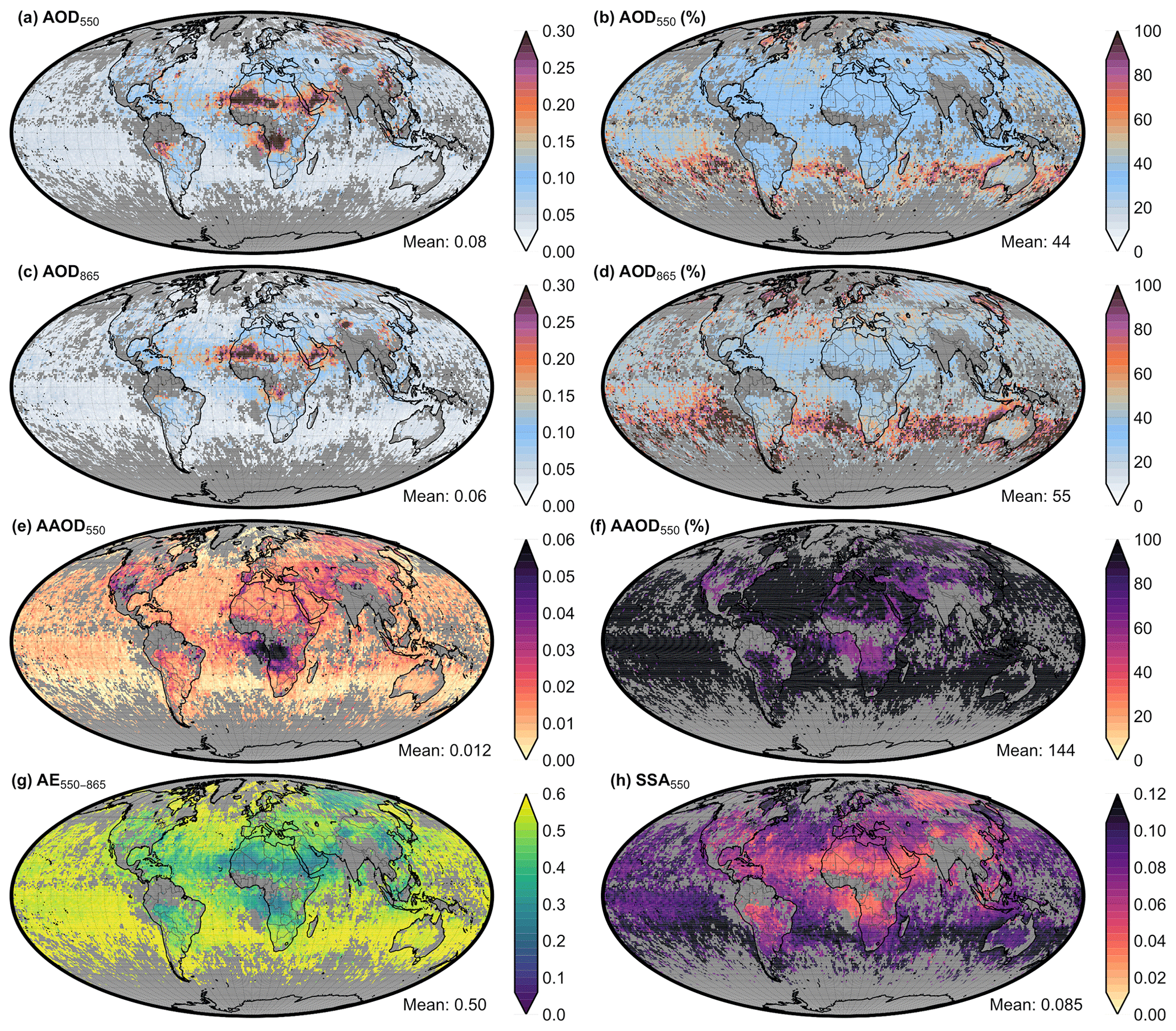
Figure 1 The uncertainty and the relative uncertainty of POLDER for AOD₅₅₀ (a, b) AOD₈₆₅ (c, d) and AAOD₅₅₀ (e, f) and the uncertainty for AE_550−865 (g) and SSA₅₅₀ (h) averaged over the period 20 July to 28 August 2006. The global mean of each variable is denoted in the bottom-right corner for each case.

In the present study, the observational uncertainties of POLDER are assessed by evaluating the retrieval against the dataset of AERONET. This approach provides a parameterization of observational uncertainty based on the real errors of POLDER retrievals. Obviously, since AERONET is a spatially sparse ground-based network of stations, some generalization had to be made as far as the performance of POLDER in remote areas. Furthermore, the AERONET retrieval errors, which typically are smaller than the errors of any remote sensing retrieval, at least for AOD, were not taken into account. A detailed description of the POLDER uncertainty estimation is presented in Appendix A.

Global maps of the resulting absolute and relative uncertainties of POLDER averaged over 40 d (the period of our assimilation experiment) for the five variables used in the present study are illustrated in Fig. 1. Also, the AERONET stations used are selected for POLDER retrievals over land, where the errors are higher in comparison to POLDER retrievals over ocean (Lacagnina et al., 2017). For the above-mentioned reasons, in cases of very low AOD₅₅₀, for example, in the first two AOD₅₅₀ bins of Fig. A1 and predominantly over ocean pixels, the POLDER uncertainty estimates are probably too conservative. The POLDER uncertainty estimation is based on spatiotemporal POLDER retrievals of a 18 km × 18 km grid with AERONET. The estimated uncertainty was afterwards applied to a coarser 1^∘ × 1^∘ grid.

The global mean absolute uncertainties for AOD in the two wavelengths (550 and 865 nm) are quite similar (0.08, 0.06), although AOD₈₆₅ is lower since the absolute values of AOD₈₆₅ are lower too. The AE_550−865 global mean absolute uncertainty is 0.50, for SSA₅₅₀ it is 0.085, and for AAOD₅₅₀ it is 0.012. It can be clearly seen that the error on AE_550−865 and SSA₅₅₀ strongly depends on AOD. For example, the error on SSA is ∼ 0.03 in regions with high aerosol loading due to biomass burning, dust outbreaks or industrial pollution but can be ∼ 0.10 over the remote ocean.

2.1.3 MODIS-DT and MODIS-DB

For a broader spatial coverage, a comparison with the independent observations MODIS Collection 5 Dark Target (MODIS-DT) and MODIS Collection 6 Deep Blue (MODIS-DB) retrievals of AOD₅₅₀ (Sayer et al., 2014) was conducted. This allows assessment of the performance of the assimilated experiments over ocean and other remote regions, away from AERONET sites. In the case of MODIS-DT, a distinctive version designed specifically for assimilation purposes was used, which was corrected using 4 years of collocated data with AERONET as a basis (Hyer et al., 2011; Shi et al., 2011; Zhang and Reid, 2006). It is noted that both MODIS-DT and MODIS-DB come with their own uncertainties; thus, the comparison with the assimilated experiments cannot be considered a validation within the strict definition of the term. The uncertainties of these products are discussed in Di Tomaso et al. (2017).

2.2 Model simulations

The atmospheric global coupled climate–aerosol modeling system ECHAM-HAM is used as the forward model to generate an ensemble of short-term forecasts. ECHAM is the general circulation part of the modeling system and it simulates the meteorological conditions of the atmosphere in a Gaussian grid, while HAM is the aerosol module that utilizes the meteorological (e.g., wind, turbulence, convection, precipitation) and surface (e.g., surface roughness, bare and vegetated surface fractions) variables of ECHAM to solve the physical and chemical aerosol particle processes.

2.2.1 The ECHAM6-HAM2 aerosol climate model

This study uses the sixth generation of the general circulation model (ECHAM6.3), which was developed at the Max Planck Institute for Meteorology (MPI-M) in Hamburg, Germany (Stevens et al., 2013). The adiabatic processes in the model are based on a spectral-transform dynamical core that simulates some essential meteorological parameters (temperature, surface pressure, vorticity and divergence) while a collection of physical schemes parameterizes the diabatic processes like convection, diffusion, turbulence and gravity waves (Schultz et al., 2018).

We employ ECHAM-HAM with a grid resolution of T63L47 (1.875^∘ × 1.875^∘, with 47 mostly tropospheric levels based on a hybrid sigma–pressure coordinate). The radiative transfer calculations in the model are performed by the Rapid Radiative Transfer Model for Global modeling (RRTM-G; Iacono et al., 2008). ECHAM can optionally force the essential meteorological parameters of its adiabatic dynamical core to approach a prescribed field by applying a relaxation technique with time-varying weights (Schultz et al., 2018). Typically, the prescribed field consists of a reanalysis database, like ERA-Interim. It is noted that the physics of the model are not directly influenced by the external nudging data; therefore, ECHAM is still the main driver of the dynamics that are just “nudged” towards a prescribed trajectory that describes the 3-D temperature, surface pressure, vorticity and divergence (Rast et al., 2015). Nudging timescales are 24 h for temperature and surface pressure, 48 h for divergence and 6 h for vorticity.

HAM simulates the physical and chemical processes of aerosol in the atmosphere (Stier et al., 2005; Zhang et al., 2012). The most recent version (HAM2.3) includes new emission schemes for aerosol and aerosol precursors and modified aerosol–cloud interactions that are summarized in Tegen et al. (2019). The M7 aerosol model used in HAM2.3 considers five groups of aerosol species: desert dust (DU), sea salt (SS), organic carbon (OC), black carbon (BC) and sulfates (SO₄) (Vignati et al., 2004). Nitrate aerosol particles (NO₃), which may be produced by gas-phase nitrate (HNO₃) and ammonia (NH₃) reactions, are not implemented in HAM2.3. Aerosols are partitioned into seven unimodal lognormal particle size distributions, called modes, separated into two hygroscopic classes (hydrophobic and hydrophilic). Six of these modes consist of an internal mix of various aerosol types. For the nucleation-mode radius, r< 0.005 µm; for the Aitken mode, it is 0.005 µm $<r<$ 0.05 µm; for the accumulation mode, it is 0.05 µm $<r<$ 0.5 µm; and for the coarse mode, it is r> 0.5 µm (Vignati et al., 2004). The cloud and aerosol optical properties are computed using Mie theory for each band of the RRTM-G and organized in lookup tables (Tegen et al., 2019). Absorption and scattering of aerosol particles in the ECHAM-HAM are calculated using the prognostic concentrations of aerosol tracers (Schultz et al., 2018).

All aerosol species are emitted, transported and deposited. Depending on their physical and chemical properties, they can take part in a number of other processes like aerosol–radiation interactions (scattering and absorption), as well as other aerosol microphysical processes (e.g., nucleation, coagulation, aerosol water uptake and cloud activation). The purely natural emitted aerosol types (DU, SS) are introduced to the atmosphere by utilizing the simulated information of ECHAM, mainly the wind and some surface and ocean characteristics. Aerosols that can be emitted or formed chemically by both natural and anthropogenic sources (OC, BC, SO₄) are introduced using predefined emission inventories (Zhang et al., 2012).

Sea salt emissions are parameterized using the wind velocity at 10 m as the dominant driver for aerosol particle production, while sea surface temperature (SST) influences mostly the emitted particles' size (Long et al., 2011; Sofiev et al., 2011). In cases where the SST is low, sea salt emissions are lower and the emitted particles are smaller compared to when SST is higher (Sofiev et al., 2011). Sea salt particles are emitted only in the soluble accumulation and coarse modes. Natural emissions of dimethyl sulfide (DMS) over the ocean, which is an aerosol precursor, are calculated online based on the 10 m wind velocity (Nightingale et al., 2000) and the prescribed concentration of DMS on the surface of the ocean (Lana et al., 2011).

Dust emissions are based on the dust source scheme developed by Tegen et al. (2002). Improvements were made in terms of the surface aerodynamic roughness length, soil moisture and soil properties specifically over East Asia by Cheng et al. (2008). Also there were updates regarding the representation of Saharan dust sources using infrared dust index from the Spinning Enhanced Visible and Infrared Imager (SEVIRI) instrument aboard the Meteosat Second Generation satellite by Heinold et al. (2016). Wind velocity at 10 m is the main driver of dust aerosol particle production, while soil properties are taken into account. Saltation processes are simulated following Marticorena and Bergametti (1995). The surface roughness length is fixed globally to a value of 0.001, and the minimum friction velocity threshold for dust mobilization is set to 21 cm s⁻¹. The threshold friction velocity depends on the soil size distribution, vegetation cover and soil moisture (Cheng et al., 2008). The preferential dust emission sources include arid or low vegetated areas and are predefined in accordance with Tegen et al. (2002). Dust particles are initially emitted in the insoluble accumulation and coarse modes, but aging processes like the condensation of sulfuric acid (H₂SO₄) onto insoluble dust particles lead to soluble dust in the accumulation and coarse modes (Zhang et al., 2012).

The emissions for the remaining aerosol types and aerosol precursors are defined using emission inventories organized into 14 sectors, with each sector corresponding to the emission flux of one or more aerosol types or aerosol precursors (Schultz et al., 2018; Tegen et al., 2019). The Atmospheric Chemistry and Climate Model Intercomparison Project (ACCMIP) dataset has been used for the anthropogenic aerosol and aerosol precursor emissions, which consists of monthly mean estimates at a horizontal resolution 0.5^∘ × 0.5^∘ (Lamarque et al., 2010). The first version of Global Fire Assimilation System (GFAS) was employed for the representation of biomass burning emissions coming from grass and forest fires. GFAS is a gridded daily product with 0.5^∘ × 0.5^∘ horizontal resolution based on the fire radiative power measurements of the MODIS instrument (Kaiser et al., 2012). The daily temporal resolution of GFAS and its accurate spatial representation of fires are the critical characteristics that make it ideal for the daily assimilation cycle applied in this study. Using standard GFAS emissions, several studies reported underestimated AOD; thus, a fire emission factor equal to 3.4 has been proposed (Kaiser et al., 2012; Tegen et al., 2019; Veira et al., 2015). This factor only corrects for the AOD bias and not the AAOD bias, and therefore the GFAS emission rescaling factor of 3.4 has not been adopted in the present study.

Most species are emitted at the lowest level of the model which represents the surface of the Earth. Aerosols related to energy production and ships are emitted directly to the second lowest level of the model. In HAM2.3, 75 % of biomass burning emissions are equally distributed in the planetary boundary layer (PBL), while 17 % and 8 % are emitted in the first and second levels above the PBL, respectively. Val Martin et al. (2010) reported that most biomass burning (BB) emissions occur within the PBL. However, it is noted that the wildfire emission height has a limited effect on global AOD distribution when compared to emission fluxes and dry or wet deposition processes (Veira et al., 2015). The partitioning of aerosol emission to the M7 modes is described in detail in Schutgens and Stier (2014). It is noted that all the experiments of this study use rescaled emissions based on the analysis of Sect. 3.4.

3 Methods

3.1 Local ensemble transform Kalman filter

In this study, we use the LETKF. The Kalman equation (Rodgers, 2000) involves the forecast, also called a priori or background state (x_b) of the system, the analysis, also called a posteriori or assimilated state (x_a) of the system, the observational data (y), the observational operator (H) and the two error covariance matrices that describe the uncertainties and correlations in the background estimates (P) and the observation estimates (R):

$$\begin{array}{}\text{(1)}& {\mathit{x}}_{\mathrm{a}}={\mathit{x}}_{\mathrm{b}}+\mathbf{G}\cdot (\mathit{y}-H\cdot {\mathit{x}}_{\mathrm{b}}).\end{array}$$

$\mathbf{G}={\mathbf{P}}_{\mathrm{a}}\cdot H^{\mathrm{T}}\cdot {\mathbf{R}}^{-\mathrm{1}}$ is called the Kalman gain. The subscripts a and b indicate the analysis and background states, respectively, and T denotes the transpose operator. Equation (1) states that the analysis state (x_a) is computed based on the background state (x_b) plus the product of the Kalman gain and the difference between the observations and the simulated observations of the background state ($\mathit{y}-H\cdot {\mathit{x}}_{\mathrm{b}}$) called innovation. Kalman gain is a matrix of weights, which corresponds to every ensemble member and adjusts the impact of innovation on the new analysis state. If Kalman gain is equal to zero, this means that either the model covariance is zero, the observational covariance error matrices is infinite, or there is no dependence of the measurements on the state vector elements, which implies that observations hold no useful information, and x_a is set equal to x_b. The analysis covariance error (P_α) can be calculated from the background state of the ensemble:

$$\begin{array}{}\text{(2)}& {\mathbf{P}}_{\mathrm{a}}={\mathbf{P}}_{\mathrm{b}}\cdot \left(\mathbf{I}+{\mathbf{P}}_{\mathrm{b}}\cdot H^{\mathrm{T}}\cdot {\mathbf{R}}^{-\mathrm{1}}\cdot H\right),\end{array}$$

where I is the identity matrix. Equations (1) and (2) can be also expressed as the minimization of the cost function:

$$\begin{array}{}\text{(3)}& \begin{array}{rl}\mathrm{\Psi }\left({\mathit{x}}_{\mathrm{a}}\right)& =({\mathit{x}}_{\mathrm{b}}-{\mathit{x}}_{\mathrm{a}}{)}^{\mathrm{T}}{\mathbf{P}}^{-\mathrm{1}}({\mathit{x}}_{\mathrm{b}}-{\mathit{x}}_{\mathrm{a}})\\ & +(\mathit{y}-H\cdot {\mathit{x}}_{\mathrm{a}}{)}^{\mathrm{T}}{\mathbf{R}}^{-\mathrm{1}}(\mathit{y}-H\cdot {\mathit{x}}_{\mathrm{a}}),\end{array}\end{array}$$

where the two components on the right side of the equation describe the difference between background and analysis states and the difference between observations and analysis state. In a nutshell, the minimization of cost function (Eq. 3) defines a new and better estimate of the state vector based on observational data, a background estimate and taking into account the errors in both the model and observations.

The comprehensive mathematical formulation of LETKF can be found at Hunt et al. (2007). LETKF was implemented by Schutgens et al. (2010a) for an aerosol application based on previous work by Miyoshi and Yamane (2007). The code was modified to operate with ECHAM-HAM and POLDER in this paper.

Table 1 State vector of the assimilation system composed by the mass mixing ratio of all the modes and species and number mixing ratio (PN) for all modes in ECHAM-HAM. Aerosols in nucleation mode are not considered in the assimilation since they contribute a very small fraction in the optical depth of aerosols.

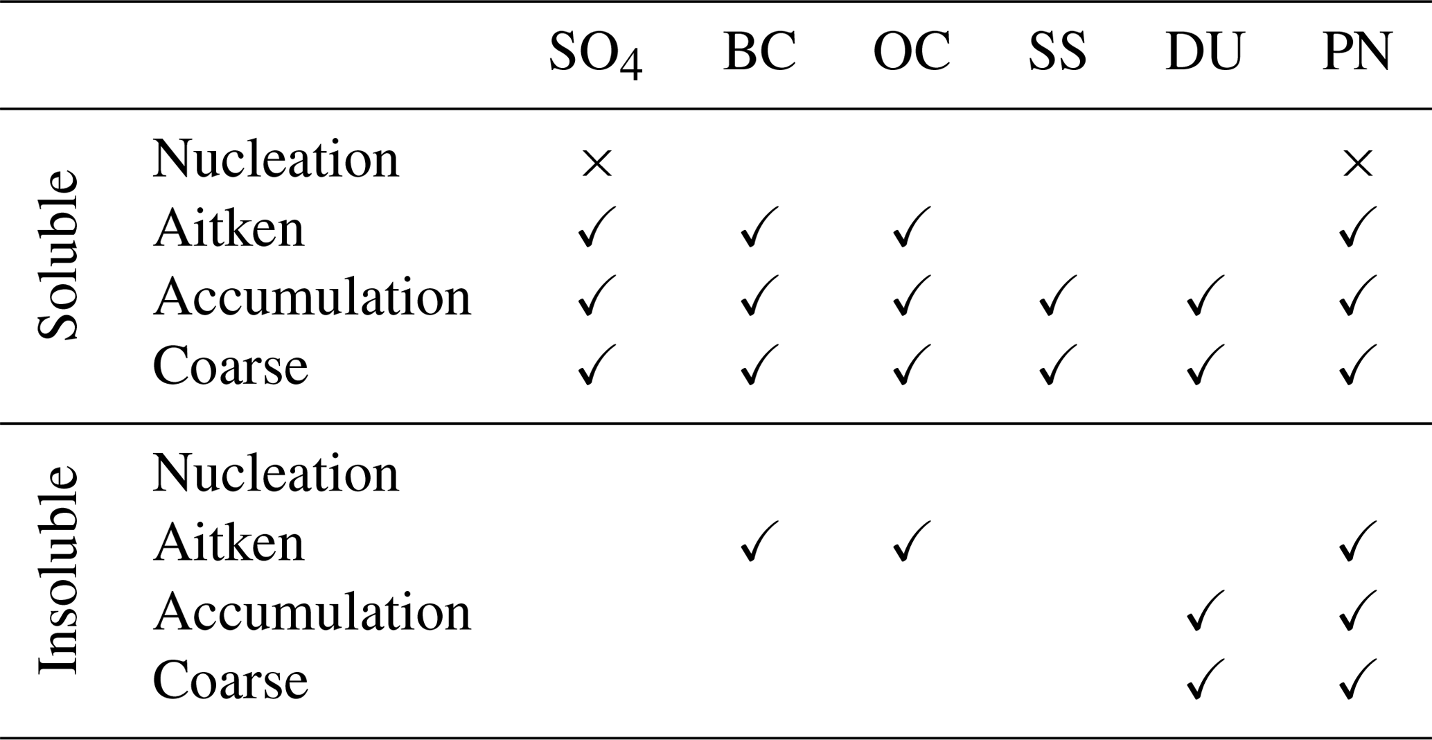
The state vector of the system (x) is in our case composed of simulated ECHAM-HAM aerosol mass mixing ratios for every mode and species and number mixing ratio for every mode (23 in total; Table 1).

The observation vector y consists of aerosol optical properties retrieved by POLDER. The observation operator H transforms the aerosol mixing ratio into simulated aerosol optical properties and uses the optical property routines in ECHAM-HAM. The perturbed ensemble of ECHAM-HAM (Sect. 3.2) embodies the model error covariance matrix P, while the calculated POLDER errors (Sect. 2.1.2) are utilized in the observation error covariance matrix R. R assumes uncorrelated between the assimilated variables; hence, the off-diagonal elements of the matrix are set to zero. In reality, correlations do exist between variables, and thus they can affect the assimilation results. The off-diagonal elements of the R matrix can be estimated by constructing a data-derived R matrix (Liu et al., 2019), but it is out of the scope of the present study.

3.2 Model uncertainties and ensemble perturbation

When creating the ensemble to represent the model error covariance matrix, we consider two sources of uncertainty: namely in the aerosol emissions and in the wind speed/direction. Global climate models or climate transport models estimates of aerosol concentration and aerosol optical properties in the atmosphere are diverse and uncertain. The most prominent cause of these uncertainties mainly originates from the emission of natural aerosols; depending on the type, global estimates may differ by a factor of 4 to 16 (Grythe et al., 2014; Huneeus et al., 2011; Lewis and Schwartz, 2004; Miller et al., 2006; Pan et al., 2019; Textor et al., 2006). A recent study highlighted that the total global emissions of OC and BC differ by a factor of 4 based on six biomass burning emission inventories (Pan et al., 2019). Furthermore, a multi-model study from AeroCom phase I (Huneeus et al., 2011) and single-model studies using different DU emission schemes (Miller et al., 2006) indicate that DU global emission fluxes may differ by up to a factor of 6. SS global emission fluxes show the highest uncertainties among all other aerosol species mostly due to the differences in the simulated particles size (Textor et al., 2006) and the differences in the sea-spray-aerosol function of the models (Grythe et al., 2014). A wide range of SS fluxes has been reported depending on the sea-spray-aerosol function used (Grythe et al., 2014), but the most well-accepted range for SS emission flux is between 1.2 and 20 Pg yr⁻¹ (Lewis and Schwartz, 2004), which implies a factor of approximately 16 SS emission flux difference between the highest and the lowest estimates.

Contrary to natural aerosol emissions, the anthropogenic aerosol emissions (OC, BC, SO₄) and their precursors (SO₂) are better constrained. For eastern China, the diversity (highest to lowest emission inventory) is lower than 1.35 for OC, BC and SO₂ (Chang et al., 2015), although for other regions like South America diversity was estimated up to 3 (Granier et al., 2011). It is noted that most anthropogenic emission inventories are used on a monthly basis; hence, the day-to-day variability is not accounted in model simulations. It stands to reason that the uncertainty in daily anthropogenic emissions should be higher than the aforementioned values derived for monthly emissions. Other studies have noted that deposition parameterization causes large uncertainties in the direct and indirect aerosol radiative effects (Lee et al., 2016; Regayre et al., 2018) and hence may be considered in our future studies.

In addition to the emission uncertainties, meteorological factors may affect the emission, transport, deposition and hence the atmospheric lifetime and radiative effect of aerosol particles. In our simulations, the surface pressure vorticity and divergence of ECHAM are nudged towards the ERA-Interim reanalysis. Although ERA-Interim is a reanalysis product that provides a better estimate of the meteorological conditions, it contains uncertainties that may affect the life cycle of aerosol particles. Several studies using wind measurements from ground stations, radiosondes, buoys, cruises ships or even satellite estimations revealed ERA-Interim errors of up to ± 3 m s⁻¹ (Bao and Zhang, 2013; Bromwich et al., 2016; Brunke et al., 2011; Campos and Guedes Soares, 2017; Stopa and Cheung, 2014).

Considering these sources of aerosol uncertainty, originating from aerosol emissions and wind speed/direction, our ECHAM-HAM forecast ensemble was assembled by multiplying the standard aerosol emissions by spatially correlated perturbations to obtain the emission for each member and by nudging each member to a slightly different version of ERA-Interim reanalysis in terms of wind speed.

A typical approach for the emission perturbation of the ensemble in past studies is to use global emission perturbations unique for each member and constant through time (Dai et al., 2014; Schutgens et al., 2010a). Another approach is to use spatiotemporal independent emission perturbations where random numbers are assigned for each grid cell, and often these numbers change in time. The latter case proved to produce very low spread in the ensemble, making the assimilation of observations impractical (Dai et al., 2014; Schutgens et al., 2010a). An intermediate approach is adopted in the present study by using spatially correlated emission perturbations, where the changes from grid to grid are not abrupt but smooth, perturbing emissions with positive or negative numbers over large areas. This technique has been successfully used in the past to derive soil erodibility factors under observation system simulation experiments (OSSEs) using an ensemble adjustment Kalman filter (Khade et al., 2013).

Spatially correlated perturbation fields are generated by first creating an ensemble (32 members in our standard setup) global grid at the resolution of the model (1.875^∘ × 1.875^∘) filled with random values, sampled from a Gaussian distribution. This spatial field of perturbations does not contain any spatial correlation between the neighboring grid cells (the spatial field for one member is shown in Fig. S1a in the Supplement). In the next step, the global grid is smoothed by averaging, for each grid box, the surrounding grid boxes that are within a two-grid-box distance (Fig. S1b). The last step is repeated five times in total (Fig. S1b–f). Next, an exponential function is applied for each grid cell separately, making the values positive and the distribution positively skewed (close to lognormal) (Fig. S1g). The final step standardizes the numbers (V) to a mean (MV_NEW) equal to the rescaled factors in Fig. S5 in the Supplement (for more information, see Sect. 3.4) and a standard deviation (SD) (SV_NEW), equal to 0.65 for each grid (Fig. S1h), in the form of

$$\begin{array}{}\text{(4)}& V_{\text{NEW}}={\text{SV}}_{\text{NEW}}\cdot {\displaystyle \frac{V-\text{MV}}{\text{SV}}}+{\text{MV}}_{\text{NEW}}.\end{array}$$

The variogram model for the spatial field of a member for each of the steps is shown in Fig. S2. According to it, in the final step (Fig. S2h), the variogram model flattens at the distance of 30^∘, which indicates that grid cells are spatially correlated up to a distance of 30^∘, whereas locations further than that are not.

The aforementioned methodology produces 32 different spatially correlated maps, one for each ensemble member. Each aerosol species has its own unique randomly generated set of 32 spatially correlated maps. The aerosol emission fluxes of the model are multiplied (perturbed) by these maps while the model runs. The SD of these spatially correlated perturbations (hence, the uncertainty of the emissions) for each species is equal to 0.65. This simplified approach assumes that the natural and anthropogenic emissions will have the same level of uncertainty.

Similar steps were followed for the creation of the zonal and meridional components of the wind spatially correlated perturbations. Contrary to the emission fluxes where numbers should be strictly positive, the wind vector sign indicates direction and the values can be negative; thus, the exponential function was not applied. The values were standardized with a mean and a SD of 0 and 0.8, respectively, using Eq. (4). The final wind perturbations are a selection of 32 members, different for the two wind components. These perturbations are added to the wind fields of the ERA-Interim reanalysis dataset, creating different perturbed branches that each member of the ensemble is nudged to. That approach can account partially for the uncertainties on the wind. A variety of other wind perturbation methods were tested, like altering the nudging relaxation time or restarting the model from different initial conditions, but were not adopted in the final experiments because either the produced ensemble spread was too small or it shrank close to zero after some days of simulation.

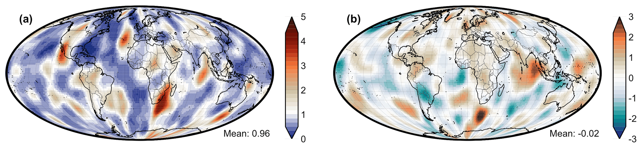
Figure 2 An example of the spatially correlated perturbations maps generated for an ensemble member regarding (a) dust emissions and (b) the U component of the wind.

The distribution of perturbations for the dust emission and U component of the wind is shown in Fig. S3. An example of the emission and wind spatially correlated perturbation maps generated for a single member is shown in Fig. 2. In this example, the DU emissions of this member are higher than the default emission parameterization over the Arabian Peninsula and the central-eastern Sahara, while the western part of the Sahara will have lower DU emissions (Fig. 2a). Similarly, the U component (positive eastward, negative westward) of the nudging data for wind over the desert will be 1 m s⁻¹ higher, which close to the surface may increase the emission of dust particles but higher up can also reduce the westward outflow of dust towards the North Atlantic (Fig. 2b). Other members may have a different combination of these parameters in the same area, which may cover other possible scenarios that may match reality.

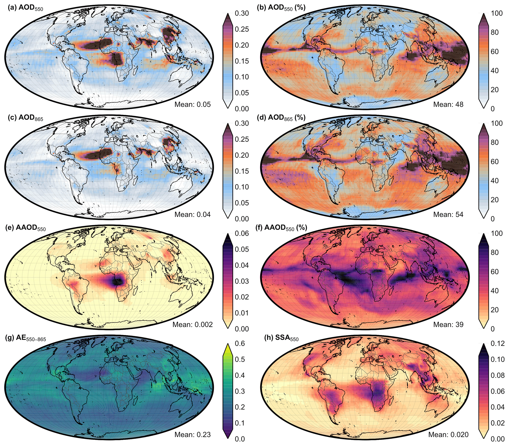
Figure 3 The uncertainty and the relative uncertainty of ECHAM-HAM for AOD₅₅₀ (a, b) AOD₈₆₅ (c, d) and AAOD₅₅₀ (e, f) and the uncertainty for AE_550−865 (g) and SSA₅₅₀ (h) averaged over the period 20 July to 28 August 2006. The uncertainty is estimated using the SD of an ensemble (32 members) where each member used different spatial correlated perturbations on aerosol emissions and wind. The relative uncertainty is defined as the ratio of SD to mean. The global mean of each variable is denoted in the bottom-right corner for each case.

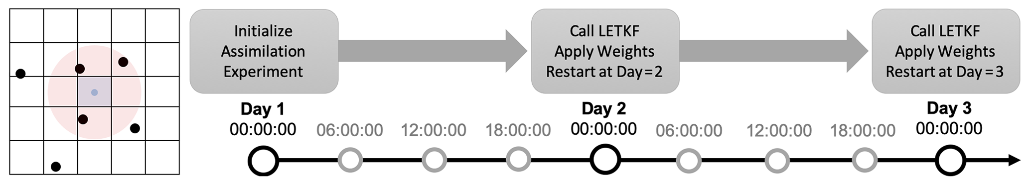
Figure 4 On the left side, the grid-cell-scale collocation of the assimilated grid and the surrounding observations is illustrated. The highlighted blue area denotes the assimilated grid cell, the red circle around it represents the local patch size (L_x), and black dots represent the observations. It is noted that in LETKF the L_x distance is represented in grid cell units, but for illustrative purposes here it is represented as a circle. On the right side, the daily assimilation cycle is depicted for 3 d.

The derived model uncertainty, shown in Fig. 3 as the SD of this perturbed ensemble, can be conceptually compared with the POLDER uncertainty (Fig. 1). In all cases, the global mean of model uncertainty is lower than the POLDER uncertainty. This does not mean that the simulated aerosol observations of the model are more accurate in comparison to POLDER. The global mean uncertainty of the model is lower since low aerosol regions (majority of points globally) are far away from emission sources. Hence, the emission perturbation has a very limited effect and the members within the ensemble are quite similar to each other in the low aerosol regions. Moreover, the global mean of the model includes polar regions where the absolute uncertainty is very low. In the remote regions, POLDER microphysical retrievals are uncertain in an absolute sense and POLDER AOD retrievals are uncertain in a relative sense. On the other hand, the exact opposite is observed close to emission sources. For example, the SSA₅₅₀ model uncertainty over the southern part of Africa can be up to 0.1 (Fig. 3h), while for the same region the POLDER uncertainty is only ∼ 0.04 (Fig. 1h). A notable difference between the model and POLDER uncertainties can be also observed for AOD₅₅₀ in any outflow region over the ocean (e.g., North Atlantic Ocean, South Atlantic Ocean, South Indian Ocean) (Figs. 1a and 3a). Furthermore, it is noted also that other uncertainty factors related to aerosol physical and chemical processes (deposition, aging, vertical convective transport) are not taken into account in our model uncertainty estimation.

3.3 Data assimilation system

Our system consists of three phases, namely the spinup, the perturbation and the data assimilation phase. The first phase includes a single simulation that runs from January 2006 to the end of May 2006 and is a spinup simulation for the ECHAM-HAM meteorological and aerosol state. The second phase consists of an ensemble of runs from June to 28 August 2006, where each member's aerosol emission (DU, SS, OC, BC and SO₄) and wind (U zonal and V meridional components) are perturbed using random spatially correlated maps (Sect. 3.2), which serves as the representation of model error in the assimilation phase. The third stage is the assimilation of observations, solved in a daily cycle from 20 July to 28 August 2006 (40 d).

The daily cycle of data assimilation involves daily forecasts (Day_t 00:00 UTC to Day_t+1 00:00 UTC) of all perturbed ensemble members. Upon completion of these simulations, the LETKF code is called, which performs a spatial collocation of the simulated (ECHAM-HAM) and the retrieved (POLDER) observations for four temporal time steps (00:00, 06:00, 12:00, 18:00 UTC). Subsequently, LETKF computes a new analysis state vector (ECHAM-HAM aerosol mixing ratio) on Day_t+1 at 00:00 UTC, which serves as the initial conditions for the next day's forecast. The process is repeated until the end of the data assimilation experiment.

At the grid cell scale, LETKF inflates the observation errors depending on their distance from the assimilated grid. This method, known in literature as “observation localization”, aims to reduce error covariance between distant points which is caused by sampling errors due to the limited ensemble size (Miyoshi and Yamane, 2007). More specifically, the local patch size (L_x) defines the distance between the analyzed grid cell and the observations that will be taken into account for assimilation. The observational error (E) of the observations that are within L_x is adjusted (E_A) according to their distance (D) in grid cell units from the assimilated grid using a horizontal correlation length (L_y):

$$\begin{array}{}\text{(5)}& E_A=E\cdot \exp \left(D/L_y^{\mathrm{2}}\right).\end{array}$$

Distant observations get higher errors and thus have a smaller contribution in the changes of the assimilated grid. In our experiments, L_x and L_y are set to 4 and 2, respectively, in grid cell units. Consequently, observations that are up to four grids (7.5^∘) away from the assimilated grid may affect the assimilated grid cell, although these more distant observations are accounted with a 2.7 times greater observational error than normal. An illustration of the daily assimilation cycle and the grid-cell-scale collocation during assimilation is depicted in Fig. 4.

3.4 Rescaling the aerosol emissions

Aerosol models often may under- or overestimate AOD₅₅₀ or AAOD₅₅₀ close to the sources. Most of these biases close to sources may be attributed to inaccurate emissions of one or two aerosol species. By rescaling these emissions by region and species, the model-simulated observations will be closer to the real observations. This rescaling of emissions can benefit the data assimilation since the Kalman filter assumes that the model is unbiased. Therefore, a simulation for 2006 was conducted with ECHAM-HAM in order to identify yearly AOD₅₅₀ and AAOD₅₅₀ biases by evaluating it against POLDER and MODIS-DT retrievals.

Initially, the mean yearly bias of the 2006 simulation against MODIS-DT AOD₅₅₀, POLDER AOD₅₅₀ and POLDER AAOD₅₅₀, as well as the yearly emission fluxes for all species were plotted (Fig. S4). The results indicate that a positive bias of the model against MODIS-DT AOD₅₅₀ is most probably driven by an overestimation of SS emission fluxes, since these two spatial patterns match (Fig. S4a and e). For the same reason, the over- or underestimation of the model when compared to POLDER AAOD₅₅₀ over wildfire or anthropogenic polluted regions may be mainly attributed to BC emission fluxes (Fig. S4c and f). Furthermore, the biases of POLDER AOD₅₅₀ over the desert are, for the most part, associated with DU emission fluxes (Fig. S4b and d). Emission rescaling factors (RFs) for SO₂, SO₄, SS and OC were based on biases against MODIS AOD₅₅₀; for DU, they were based on biases against POLDER AOD₅₅₀; and for BC, they were based on biases against POLDER AAOD₅₅₀ (Fig. S5). The emission RFs were calculated as the ratio of observations (OBS) to model (MOD) AOD₅₅₀ or AAOD₅₅₀ for each region (r):

$$\begin{array}{}\text{(6)}& {\text{RF}}_{\mathrm{r}}={\displaystyle \frac{{\text{OBS}}_{\mathrm{r}}}{{\text{MOD}}_{\mathrm{r}}}}.\end{array}$$

Afterwards, the global grid was smoothed to avoid spatially steep changes of aerosol emission fluxes by averaging each grid cell with the surrounding values at a distance of two grid cells. This approach does not account for observation errors, it does not consider the interannual and intra-annual biases, and it is noted that the aerosol emission adjustment is based on AOD₅₅₀ and AAOD₅₅₀ biases, which may not be directly related to aerosol emissions.

An obvious limitation of this method occurs over the Southern Hemisphere major fire sources, where AOD₅₅₀ is underestimated and AAOD₅₅₀ is overestimated by ECHAM-HAM. Following the above-mentioned methodology, the resulting emission factors for fire source regions of the Southern Hemisphere would result in a reduction of BC emission fluxes by 10 %, due to the underestimation of AAOD₅₅₀, and an increase of OC emission fluxes by more than 50 %, due to the underestimation of AOD₅₅₀. The outcome would provide an improvement in terms of AOD₅₅₀ but not for AAOD₅₅₀, since part of the AAOD₅₅₀ (10 %–20 %) emerges from other species, like OC. Thus, in order to get a simultaneous improvement in both AOD₅₅₀ and AAOD₅₅₀, OC emission fluxes were not adjusted in wildfire regions in the Southern Hemisphere major fire regions (Fig. S5c). The emission perturbation of the ensemble that is used in the core experiments is up to 3 times greater than the rescaling factors applied in this stage; thus, the high and low values of the original unadjusted yearly simulation are still represented in the perturbed ensemble.

3.5 Experimental setup

The experiments are focused on the summer of 2006, and assimilation is performed for the period of 20 July to 28 August 2006. The year was selected according to the availability of POLDER SRON retrievals, while the summer season was chosen due to the high peak of forest fires in the tropical band and the pronounced dust plume over the Atlantic, where AAOD and AE in the model can benefit from the assimilation process. The model simulations were bilinearly interpolated when necessary to a 1^∘ × 1^∘ global grid for a direct comparison with the gridded satellite retrievals.

The core experiments presented in Sect. 4.1 assess the potential added value of assimilating aerosol information related to the size and absorption. In the CONTROL experiment, there was no assimilation of any kind of observations. In the MASS experiment, only AOD₅₅₀ was assimilated. In the SIZE1 and SIZE2 experiments, either AOD₅₅₀ and AOD₈₆₅ or AOD₅₅₀ and AE_550−865 were assimilated, respectively. In the ABSORB1 and ABSORB2 experiments, either AOD₅₅₀ and AAOD₅₅₀ or AOD₅₅₀ and SSA₅₅₀ were assimilated, respectively. Finally, the TOTAL experiment assimilates AOD₅₅₀ and AE_550−865 and SSA₅₅₀.

Table 2 The name along with the assimilated aerosol optical properties and the physical meaning of each experiment. All the assimilated parameters are retrievals of POLDER. All of the experiments used the rescaled emission factors of Sect. 3.4.

Sensitivity experiments described in Sect. 4.3 intend to explore LETKF's sensitivity to three main parameters: ensemble size (n_ens), local patch size (L_x) along with horizontal correlation length (L_y) and inflation factor (ρ) following an analogous analysis conducted by Schutgens et al. (2010b). The n_ens is essentially the number of members used in ensemble and is connected to the accuracy and diversity of the model-predicted covariant error. The L_x represents the distance around a model grid that defines whether an observation would be considered in the assimilation process, while ρ relates to a technique that multiplies the error covariance matrix of the ensemble to increase the ensemble spread and ensure that the assimilation of new observations is possible in the next assimilation step (because otherwise the ensemble spread decreases during the assimilation process). Table 2 presents a summary of the core and the sensitivity experiments.

4 Results

4.1 Comparison to POLDER observations

We first evaluate the impact of data assimilation by evaluating the daily forecast, starting from the latest analysis, with POLDER data not yet assimilated. The benefit of this sort of evaluation is that biases in POLDER retrievals are effectively removed (because the observations used for either assimilation or evaluation come from the same POLDER dataset), and one can study the merits of data assimilation without the added issue of observational biases. The drawback is that such an evaluation cannot determine if the assimilation of POLDER retrievals actually yields improved aerosol simulation. The evaluation of the system with completely independent observations is presented in Sect. 4.2. Each experiment consists of an ensemble of simulations. The ensemble mean of each experiment is the best estimate for the state vector and the simulated observations. Thus, only the ensemble mean of each experiment is presented in the results. Throughout the results, we use the forecast run of the most recent analysis.

Figure 5 Aerosol Optical Depth at 550 nm for (a) POLDER, the (b) CONTROL, (c) MASS, (d) SIZE2, (e) ABSORB2, (f) TOTAL experiments and their differences (model – POLDER; g–k). All fields are spatiotemporally collocated to the available measurements of POLDER for the period 20 July to 28 August 2006. Grey-filled grid cells indicate the absence of any valid POLDER measurements for the study period.

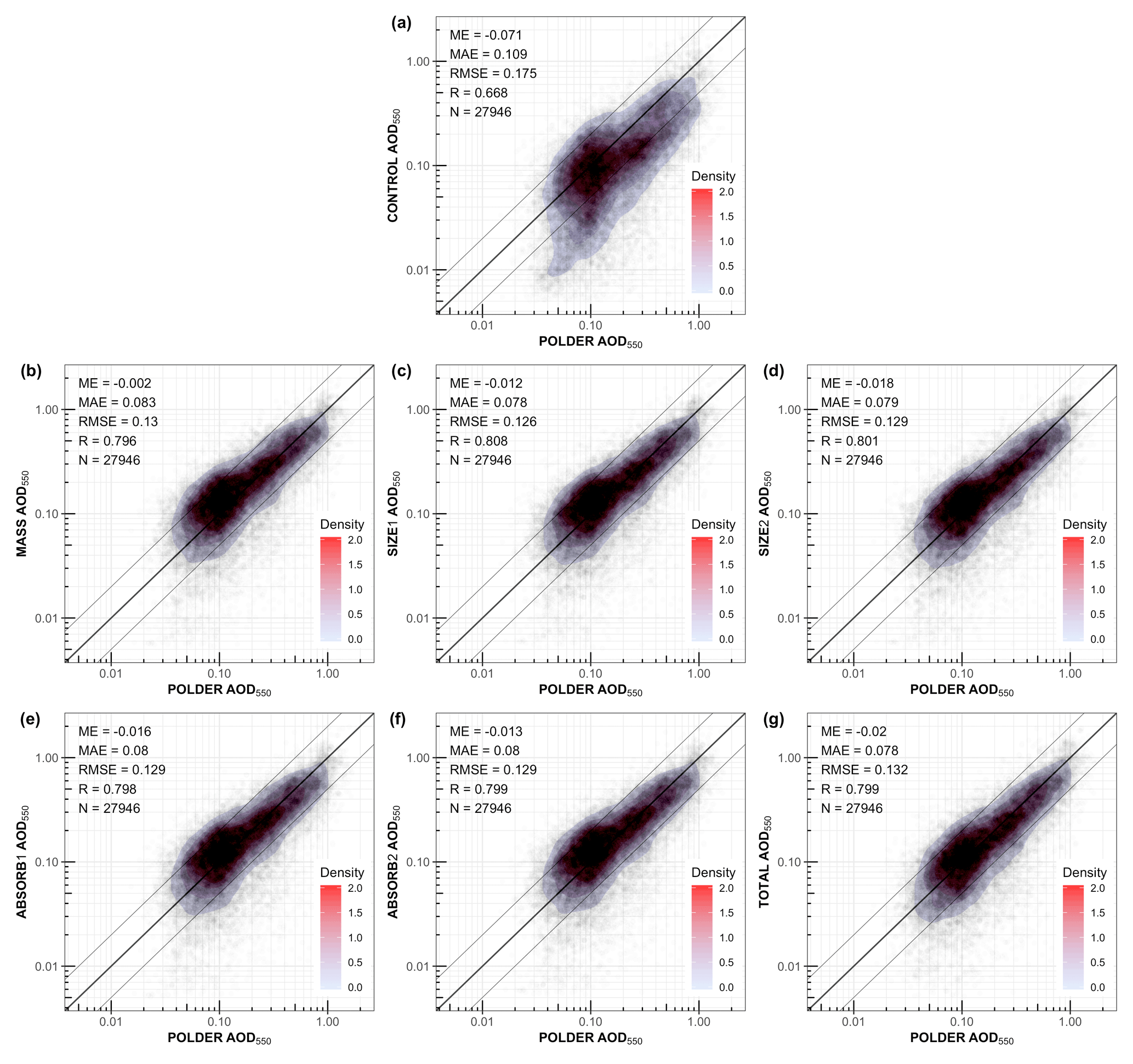
Figure 6 Aerosol optical depth at 550 nm of POLDER against the core experiments, regarding all the available points of POLDER for the period 20 July to 28 August 2006. In each subplot, the bold line indicates the perfect model (y=x), while the two thinner lines confine the −200 % and 200 % bias boundaries, respectively. The shade depicts the density of points. N represents the total number of points.

4.1.1 Aerosol optical depth

Figures 5 and 6 show the AOD₅₅₀ fields for the different data assimilation experiments of Table 2 and their agreement with the POLDER AOD₅₅₀. Looking at the CONTROL experiment, we see that the model underestimates AOD₅₅₀ over land in most regions with high AOD₅₅₀, such as the Sahara (dust), tropical Africa (biomass burning) and Asia (industrial). On the other hand, over ocean the model has the tendency to overestimate AOD₅₅₀. Overall, the global mean AOD₅₅₀ of the model (0.146) is substantially lower than that of POLDER (0.228).

When assimilating AOD₅₅₀ (MASS experiment), the global bias virtually disappears, which indicates the data assimilation system is capable of using the AOD₅₅₀ information provided by POLDER measurements. When more properties than just AOD₅₅₀ are assimilated (SIZE2, ABSORB2, TOTAL), the bias in AOD₅₅₀ gets a bit larger than when only assimilating AOD₅₅₀ (−0.013 to −0.020) but is still much smaller than for the CONTROL experiment. The reason that the agreement with POLDER AOD₅₅₀ gets slightly worse when assimilating other properties in addition to AOD₅₅₀ (AE and/or SSA) is that the system needs to find the best compromise in fitting all properties simultaneously. So, in some situations the only way to get a better fit to AE is to degrade the fit to AOD₅₅₀ (because of different assumptions used in the model).

Overall, local biases are decreasing after assimilation; however, over certain areas, biases can be increased, for example, over the South Atlantic Ocean in the MASS experiment (Fig. 5h). The assimilated AOD₅₅₀ over Africa in the tropics increases the aerosol mixing ratio over land, which is then transported westward over the South Atlantic. The assimilation of AOD₅₅₀ over the South Atlantic should compensate some of that effect by decreasing the aerosol mixing ratio but evidently not sufficiently. The assimilation of other aerosol optical properties like AE_550−865 and SSA₅₅₀ reduces the South Atlantic positive AOD₅₅₀ bias, especially in the case of the TOTAL experiment (Fig. 5k), indicating that the simultaneous assimilation of multiple variables can improve the simulated AOD₅₅₀ spatial representation in some places.

The AOD₅₅₀ scatterplots for all core experiments are depicted Fig. 6. The averaged global mean error (ME) is reduced from −0.071 in the CONTROL to values that range between −0.002 to 0.020 in the assimilated experiments. Similarly, the mean absolute error (MAE) is reduced from 0.109 in the CONTROL to 0.078 in the TOTAL experiment. Pearson's correlation (R) increases from 0.668 to approximately 0.8 for all assimilated experiments. The consistent improvement of AOD₅₅₀ in the assimilation experiments demonstrates that the combination of assimilated observations does not negatively affect AOD₅₅₀.

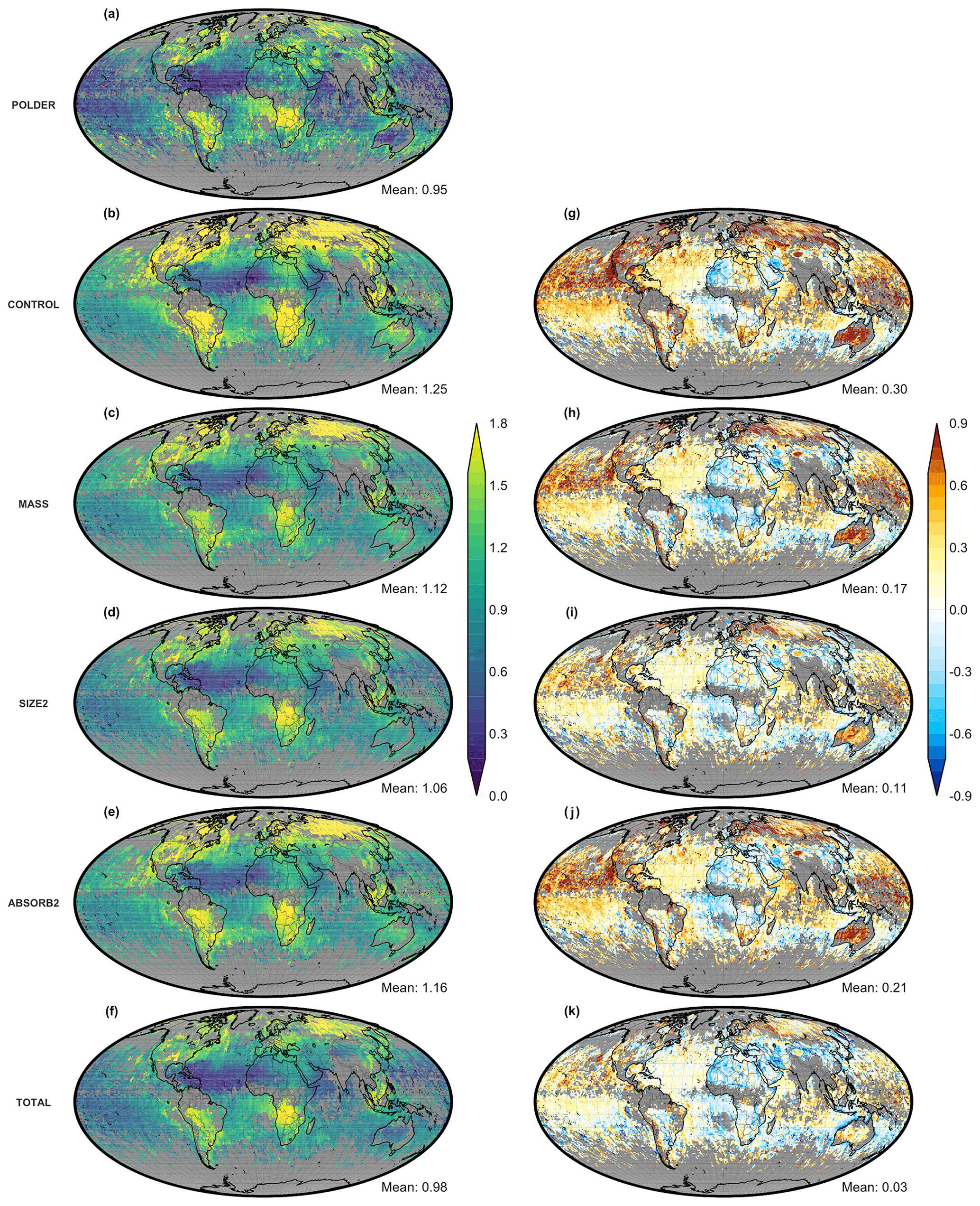
Figure 7 Similar to Fig. 5 but for the Ångström exponent at 550–865 nm.

Figure 8 Similar to Fig. 6 but for the Ångström exponent at 550–865 nm. The two thinner lines confine the −30 % and 30 % bias boundaries, respectively.

4.1.2 Ångström exponent

Figures 7 and 8 depict AE_550−865 for POLDER and the data assimilation experiments. The CONTROL experiment overestimates the AE_550−865 in most cases (Pacific and Indian oceans, Australia, Siberia) and underestimates it in the western Sahara. Globally, the mean AE_550−865 of CONTROL (1.25) is higher than that of POLDER (0.95), which indicates that the model overestimates the ratio of fine- to coarse-mode particles.

The MASS experiment has lower global AE_550−865 (1.12), which matches slightly better but still remains higher than POLDER. In the MASS experiment, only AOD₅₅₀ is assimilated; thus, any information regarding size or chemical composition will be related to a combination of transport and previous cycles that assimilated AOD₅₅₀ close to sources. More specifically, particle size information may indirectly be introduced into the assimilation system by adjusting the AOD of two neighboring regions with different dominant particle size distributions, like northern Africa and Europe. For example, in Europe, the spatial averaged bias of AE_550−865 in the CONTROL experiment was 0.20, while in MASS it is 0.01 (Fig. S6).

The other experiments (SIZE2, ABSORB2 and TOTAL) reduce the global mean of AE_550−865 even more (1.06, 1.16 and 0.98, respectively). The combined information of more observations related to mass, size and absorption reduces the local biases of AE_550−865 as well as the global ME and MAE while increasing R (Fig. 8g). Also, in the TOTAL experiment, the AE_550−865 is improved substantially even in areas where the POLDER uncertainty of AE_550−865 is quite high. For example, the POLDER uncertainty in Australia is approximately 0.5 (Fig. 1g), but CONTROL overestimates AE_550−865 by 0.8 over land (Fig. 7g).

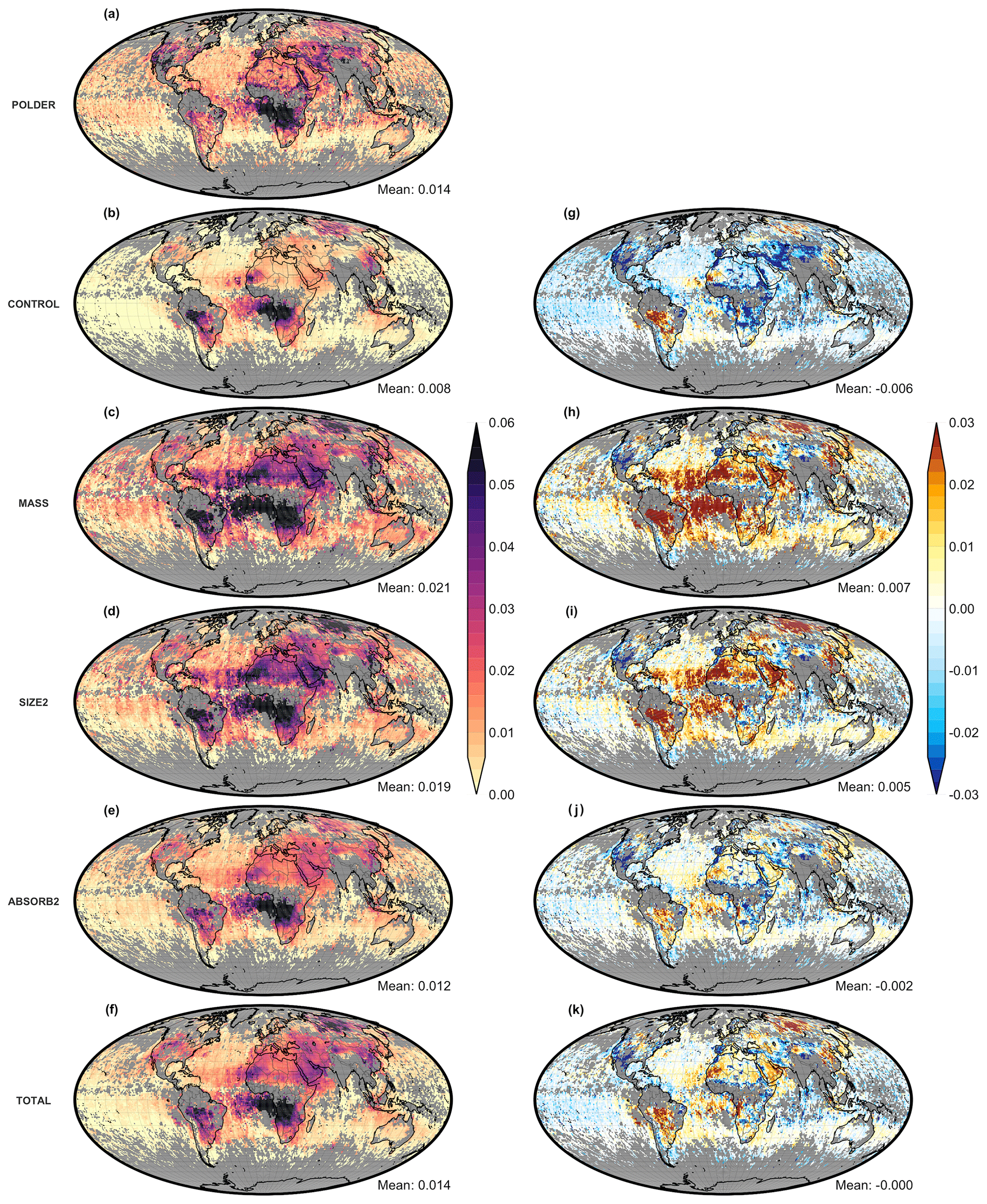
Figure 9 Similar to Fig. 5 but for absorption optical depth at 550 nm.

Figure 10 Similar to Fig. 5 but for single scattering albedo at 550 nm.

Figure 11 Similar to Fig. 6 but for aerosol absorption optical depth at 550 nm.

4.1.3 Aerosol absorption

Figures 9 and 10 show the agreement in AAOD and SSA, respectively, between the different experiments and the POLDER observations. The CONTROL experiment shows lower global mean aerosol absorption than the POLDER observations; i.e., the AAOD is lower and the SSA is higher. Regionally, the differences are more complex. For example, over the southern part of Africa, with a lot of biomass burning, the AAOD is low compared to POLDER, and the SSA is as well. This means that the difference in AAOD is mostly caused by too-low total AOD but that the aerosols are more absorbing “per particle” in the CONTROL experiment than in POLDER. A similar pattern is observed over northern Eurasia. On the other hand, over the Middle East and over North America, a low bias in AAOD is observed together with a high bias is SSA, while for South America a high bias in AAOD is observed together with a low bias in SSA. So, in these regions, the differences between POLDER and the CONTROL experiment are caused by differences in absorption properties of the aerosols.

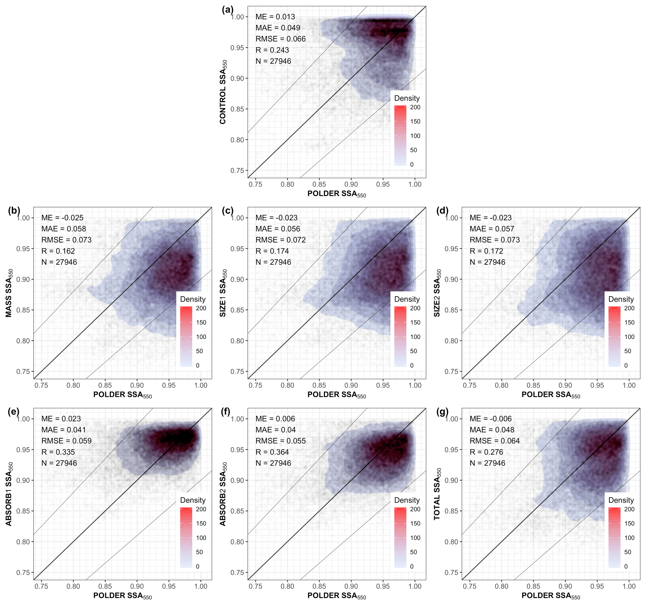
Figure 12 Similar to Fig. 6 but for single scattering albedo at 550 nm. The two thinner lines show the −10 % and 10 % bias boundaries, respectively.

It is interesting to note that in the MASS experiment the AOD₅₅₀ is improved (Fig. 5h) but SSA₅₅₀ and AAOD₅₅₀ not so much, especially in regions like South America, Africa and the Atlantic Ocean (Figs. 9h and 10h). The reason behind that is easiest to explain over South America, where AOD₅₅₀ is underestimated and AAOD (SSA) is overestimated (underestimated) in CONTROL. The assimilation of AOD₅₅₀ (MASS) will increase the aerosol mixing ratio of all aerosols based on their extinction, but it will not be based on their absorption. Thus, AAOD will be increased along with AOD since more aerosols will be in the atmosphere. Specifically, in the Amazon basin, SSA₅₅₀ of the MASS experiment decreases by 0.032 in comparison to CONTROL, since the BC column burden becomes 4 times higher (Fig. S7b), while the difference of SSA₅₅₀ between POLDER and the model (spatiotemporal collocated points only) increases from −0.084 to −0.117 (Fig. S7c).

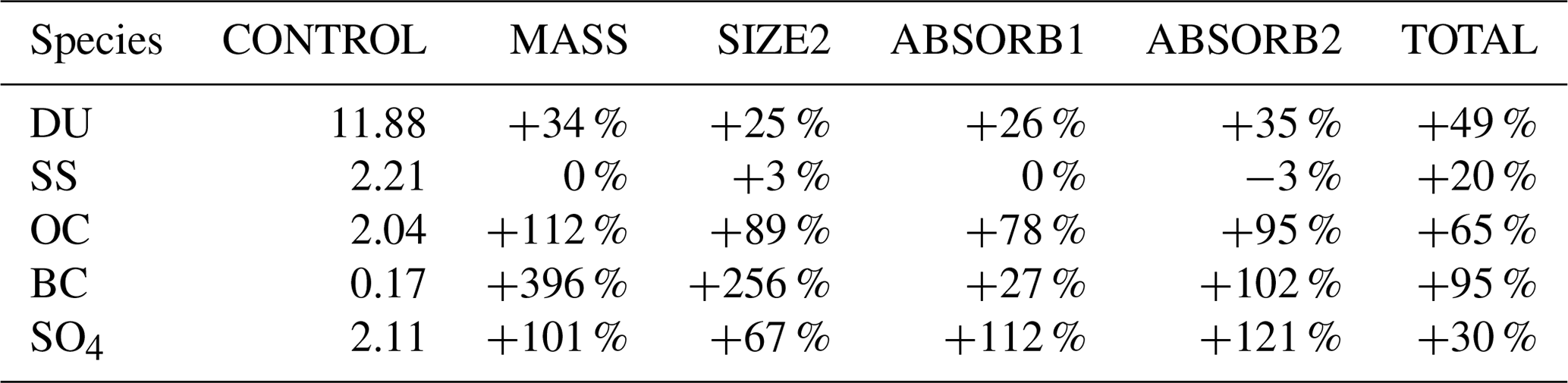
Table 3 Global column burden (Tg) of all aerosol species regarding the CONTROL experiment and the induced percentage changes due to assimilation for the MASS, SIZE2, ABSORB1 and TOTAL experiments.

Scatterplots of all experiments for AAOD₅₅₀ and SSA₅₅₀ are depicted in Figs. 11 and 12, respectively. The global SSA₅₅₀ ME gets worse from 0.013 to −0.025 for the MASS experiments, the MAE increases also from 0.049 to 0.058, while R decreases from 0.243 to 0.162 (Fig. 12a and b). These results reveal the limitations of an aerosol data assimilation system that assimilates AOD in only one wavelength. Assimilating size information does not really improve the agreement in AAOD or SSA, but as expected, when assimilating SSA (ABSORB2 experiment), the agreement between model and POLDER data significantly improves for both AAOD and SSA. This improvement is maintained for the TOTAL experiment, assimilating AOD, AE and SSA together. The SSA₅₅₀ of ABSORB2 experiment is still slightly higher over the Amazon basin and lower in the Middle East (Fig. 10j), but overall the simulated absorbing properties are significantly better in comparison to the CONTROL experiment (Fig. 10g) and much better in comparison to the MASS experiment (Fig. 10h).

4.1.4 Aerosol column burden changes

The aerosol column burden changes for each experiment are depicted in Table 3. All experiments reveal that ECHAM-HAM underestimates aerosol column burden globally; thus, the changes for all species are positive. In the MASS experiment, BC column burden is almost 5 times greater than the CONTROL experiment. BC AOD₅₅₀ contribution to AOD₅₅₀ is less than 10 % in most regions over the globe; thus, the assimilation of only AOD₅₅₀ should not affect the BC column burden significantly. On the other hand, OC AOD₅₅₀ contribution to AOD₅₅₀ is between 50 % and 90 % in the tropical fire and outflow areas, and thus the assimilation of AOD₅₅₀ is expected to significantly affect the OC column burden. Although BC and OC emissions are perturbed differently, correlations in these two species will still persist, since both BC and OC are emitted from the same location (but not with the same magnitude) and are following similar transport paths in each member. Thus, we conclude that the large BC column burden increase is related also to the correlations between OC and BC AOD₅₅₀. The ABSORB1 experiment constrains the BC increase to +27 % in comparison to CONTROL. The TOTAL experiment increases of the column burden range between +20 % and +95 % for all the species. To understand better how these changes are made, we explore further regionally by isolating the effect of assimilating AE_550−865 and AAOD₅₅₀ for Australia and South America, respectively.

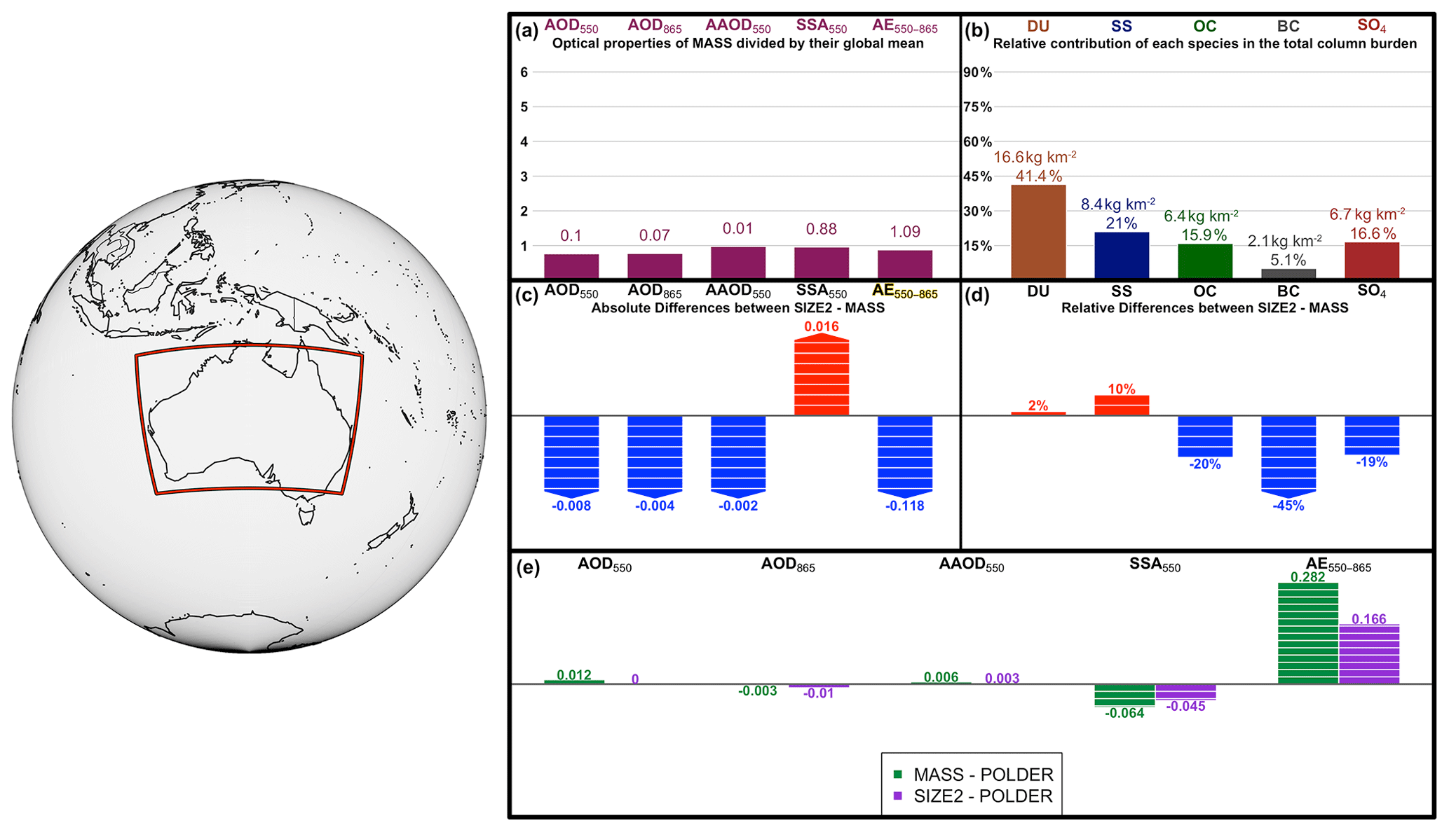
Figure 13 An overview of the changes due to the addition of POLDER AE_550−865 in the assimilation for Australia. Panel (a) depicts the mean values of five aerosol optical properties, while the height of bars indicates the regions relative amount of each property in comparison to the global mean. Panel (b) illustrates the column burden of five aerosol species as simulated in the MASS experiment. The percentage in the column burdens of each species specifies the relative contribution of each species in the total column burden. Panel (c) illustrates the absolute changes caused in aerosol optical properties, due to the assimilation of AE_550−865 (SIZE2 – MASS), while the height of bars indicates if the change is just positive or negative. Panel (d) shows the relative changes caused in the mixing ratio for each species due to the assimilation of AE_550−865 (SIZE2 – MASS). Panel (e) displays the aerosol optical properties' bias in comparison to POLDER for the MASS and SIZE2 experiments.

Figure 13 depicts the aerosol optical properties and aerosol column burden changes over Australia caused by the assimilation of AE_550−865 by subtracting the value for the MASS experiment from SIZE2 (SIZE2 – MASS). Australia is a mixed aerosol area with fairly low aerosol content and many uncertain emission sources within the continent, while satellite retrievals are quite diverse (Schutgens et al., 2020) due to the complex surface albedo of the continent. MASS clearly overestimates the amount of fine particles over the Australian continent compared to POLDER (Fig. 7h); hence, the addition of AE_550−865 in the assimilation increases the column burden on rather coarser aerosol groups (DU and SS) and decreases the column burden the modes corresponding to fine particles, where OC, BC and SO₄ are dominant. (Fig. 13c). Consequently, the AE_550−865 bias against POLDER is reduced from 0.282 in the MASS experiments to 0.166 in the SIZE2 experiment. The bias is decreased also in some other parameters, like AOD₅₅₀, AAOD₅₅₀ and SSA₅₅₀. It is noted that the aerosol mixing ratio changes on the assimilation system are conducted for every aerosol tracer separately (Table 1), but since some aerosol groups contain higher column burden in coarser aerosol modes (DU and SS) and others in finer aerosol modes (OC, BC, SO₄), aerosol adjustments due to assimilation are regularly consistent (either positive or negative) for an aerosol species as a whole, like in the case of Australia.

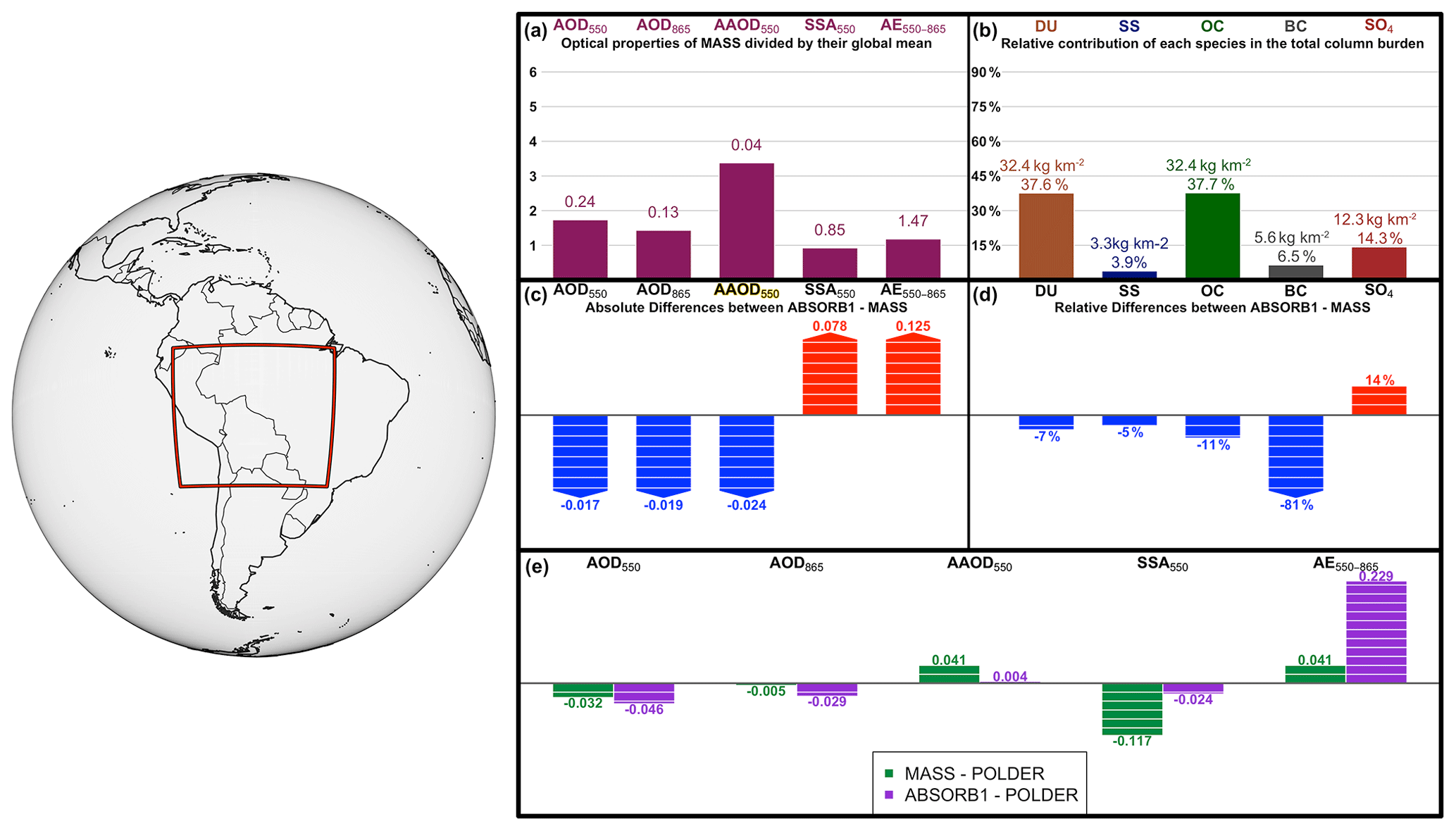
Figure 14 Similar to Fig. 13 but for South America. The depicted experiments are MASS and ABSORB1; hence, the changes in panels (c) and (d) are based on the addition of AAOD₅₅₀ to the assimilation.

Similarly, Fig. 14 depicts the aerosol optical properties and aerosol column burden changes over South America caused by the assimilation of AAOD₅₅₀ by subtracting the MASS experiment from ABSORB1 (ABSORB1 – MASS). South America, and specifically the Amazon basin, is a major active burning area of the globe in July and August with significant emissions of absorbing aerosol particles. When assimilating AOD₅₅₀ and AAOD₅₅₀ (ABSORB1), the absorption optical properties are improved (Fig. 14c), while the AOD₅₅₀, AOD₈₆₅ and AE_550−865 performance slightly deteriorates. The changes in the simulated absorbing properties are mainly driven by a −81 % reduction of the BC mixing ratio, which reduces the AAOD₅₅₀ by −0.024 and increases the SSA₅₅₀ by 0.078 in comparison to the MASS experiment (Fig. 14b). DU and OC changes may in the ABSORB1 experiment affect a small fraction of AAOD₅₅₀ changes too, but predominantly the other species adjust to match the other assimilated parameter (AOD₅₅₀) as well as possible.

4.2 Comparison with the independent observations

In this subsection, we evaluate the aerosol fields from the different data assimilation experiments using independent observations. AERONET is the most important data source for this purpose given its high accuracy, especially for AOD from its direct-Sun product. However, spatial coverage by AERONET sites is sparse and entirely absent over the ocean (except for a few islands and coastal stations). MODIS-DT and -DB on the other hand provide close-to-global coverage and have been extensively evaluated. Here, we present the comparisons of our POLDER assimilation experiments with these independent datasets.

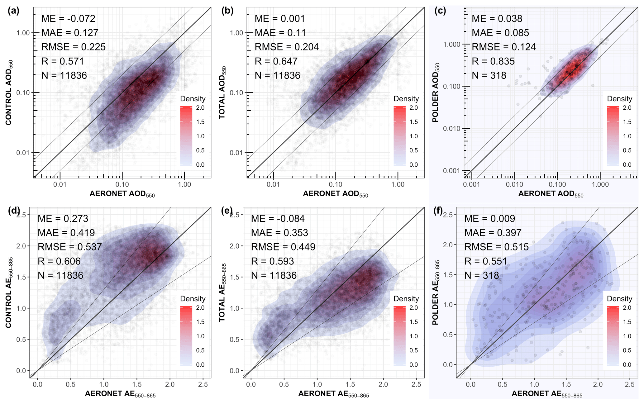
Figure 15 Comparison between the AERONET (direct-Sun V3 L2) and the CONTROL, TOTAL and POLDER experiments for AOD₅₅₀ (a–c) and AE_550−865 (d–f).

4.2.1 Evaluation with AERONET

In Fig. 15, the background simulation (CONTROL) and the total aerosol assimilated experiment (TOTAL) are evaluated against AERONET direct-Sun V3 L2 dataset for AOD and AE. The background simulation (CONTROL) shows a clear negative bias with AERONET in AOD of −0.072. Assimilating POLDER AOD, AE and SSA simultaneously (TOTAL) removes this bias almost entirely (remaining bias of 0.001). The reduction in MAE is much more moderate (from 0.127 to 0.11). In terms of AE_550−865, the ME is reduced from 0.273 to −0.084, and the MAE is reduced from 0.419 to 0.353 (Fig. 15d and e). The spatiotemporal collocated points between POLDER and AERONET indicate that POLDER has a very small ME in AOD₅₅₀ and AE_550−865 (Fig. 15c and f); thus, the assimilation of these variables from POLDER will converge the ensemble mean to a very low bias in comparison to AERONET (Fig. 15b and e).

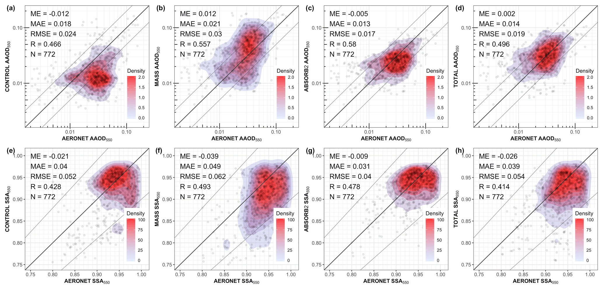
Figure 16 Comparison between the AERONET (aerosol inversion V3 L2) and the CONTROL, MASS, ABSORB2 and TOTAL experiments for AAOD₅₅₀ (a–d) and SSA₅₅₀ (e–h).

In Fig. 16, the CONTROL, MASS, ABSORB2 and TOTAL experiments are evaluated using the AERONET aerosol inversion V3 L2 dataset for AAOD₅₅₀ and SSA₅₅₀. Both properties deteriorate in the MASS experiment and improve in the ABSORB2 experiment (Fig. 16b and e), while in TOTAL experiment only AAOD₅₅₀ improves (Fig. 16c and f). It is noted that the AERONET aerosol inversion dataset that provides AAOD₅₅₀ and SSA₅₅₀ contains far fewer stations and hence less collocated points with the model (N = 772), in comparison to the AERONET direct-Sun dataset (N = 11 832). The spatiotemporal collocated points of POLDER retrievals with the AERONET inversion V3 L2 dataset were very few (N = 31) for the study period and thus are not shown.

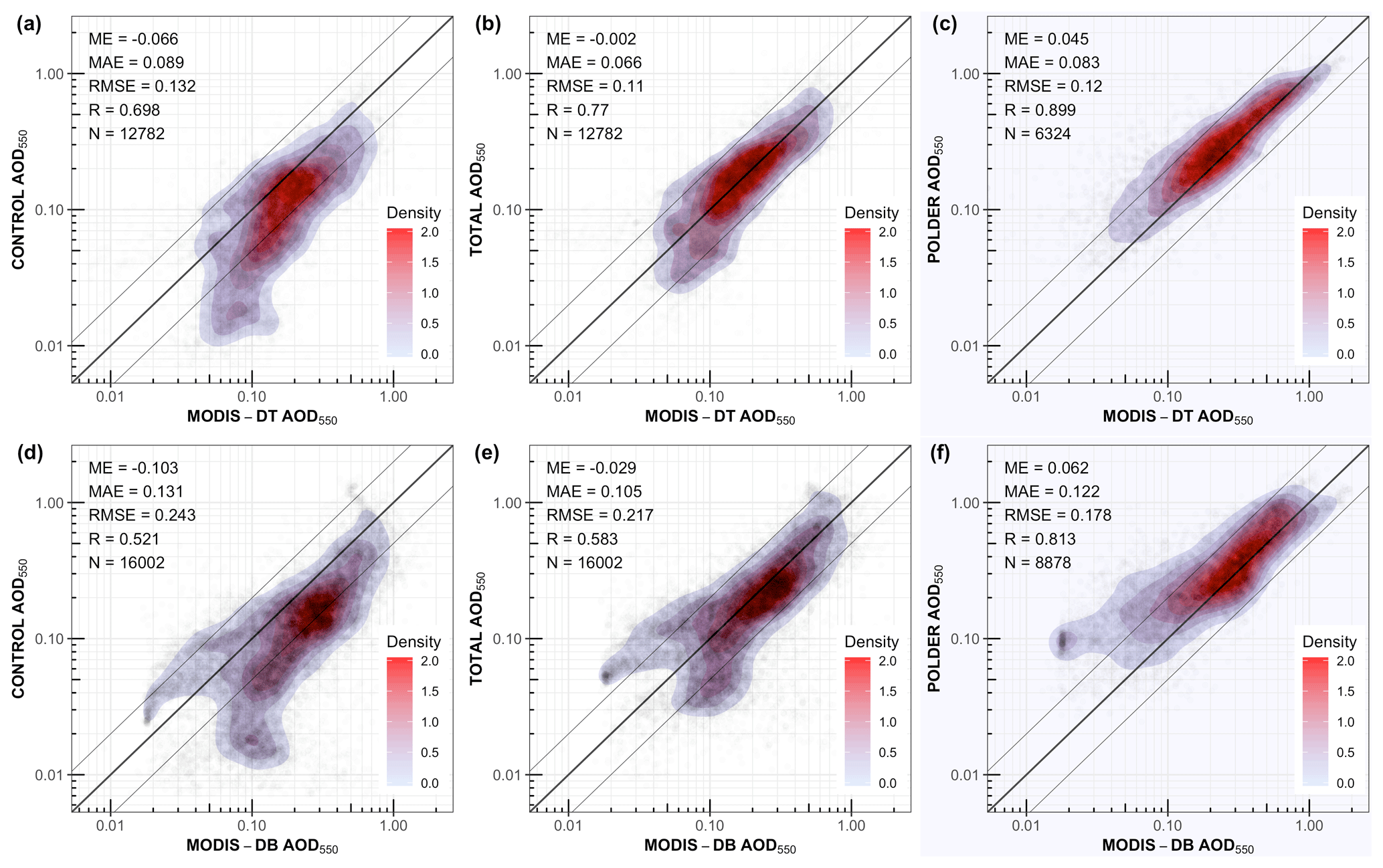
Figure 17 The AOD₅₅₀ of MODIS-DT over land against the CONTROL, TOTAL and POLDER experiments (a–c). Similar setup for MODIS-DB AOD₅₅₀ (d–f).

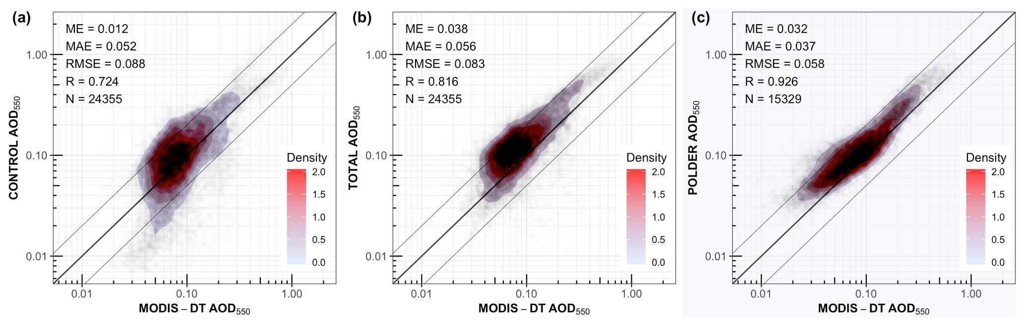
Figure 18 The AOD₅₅₀ of MODIS-DT over ocean against the CONTROL, TOTAL and POLDER experiments (a–c).

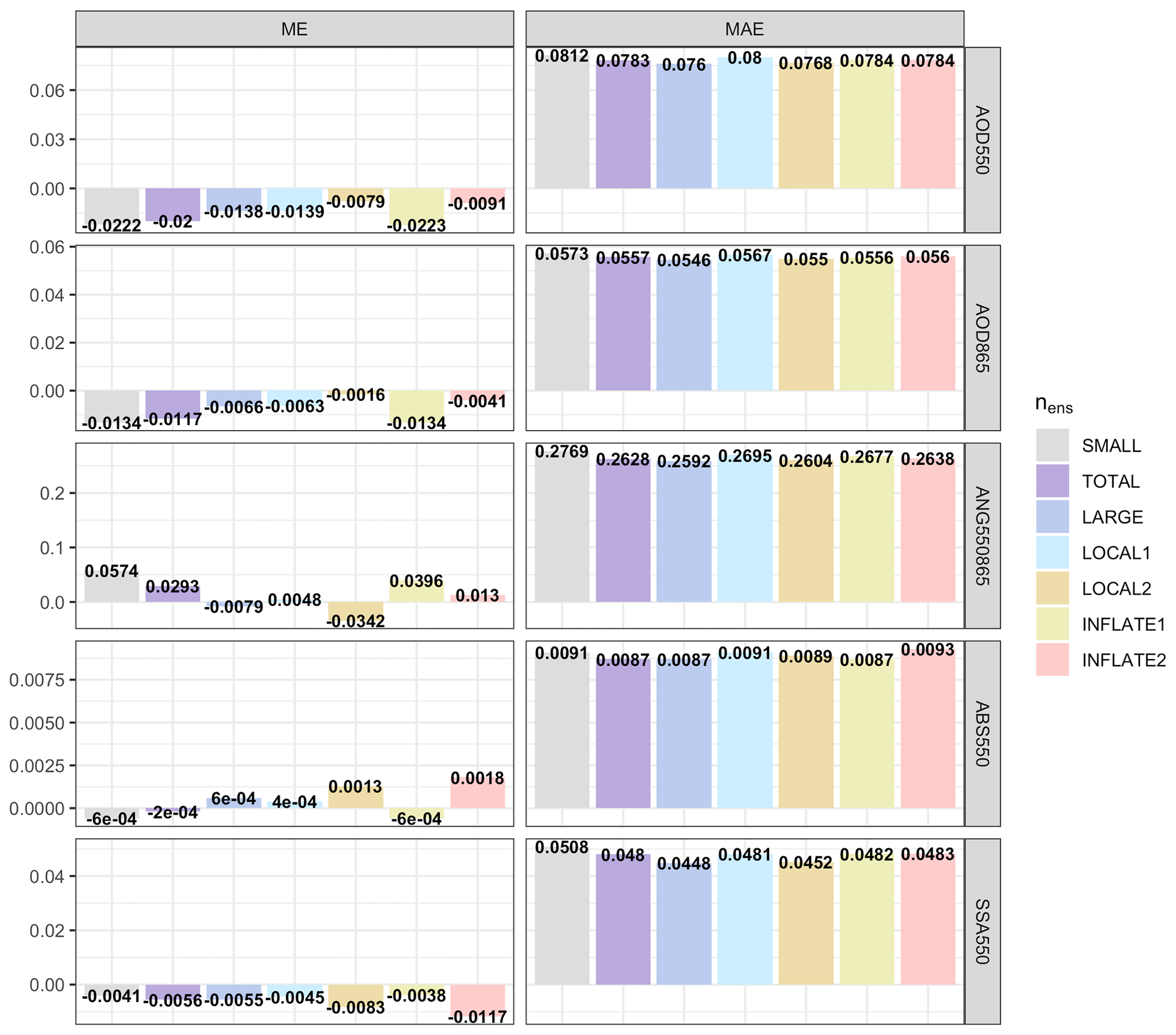
Figure 19 ME and MAE for all the spatiotemporal collocated points between POLDER (assimilated observations) and the experiments, averaged over the whole study period.

Figure 20 ME and MAE for all the spatiotemporal collocated points between AERONET (independent observations) and the experiments. AOD₅₅₀, AOD₈₆₅ and AE_550–865 are calculated using the AERONET direct-Sun V3 L2 dataset, while AAOD₅₅₀ and SSA₅₅₀ are calculated using the AERONET aerosol inversion V3 L2 dataset.

4.2.2 Comparison with MODIS-DT and MODIS-DB

The AOD₅₅₀ of the CONTROL and the TOTAL experiments is compared with MODIS-DT and MODIS-DB over land in Fig. 17. In both cases, the negative ME is reduced in the assimilated experiment from −0.066 to −0.002 (MODIS-DT over land) and −0.103 to −0.029 (MODIS-DB); the MAE is reduced as well and the correlation increases. The assimilation of POLDER observations brings the analysis closer to MODIS-DT and MODIS-DB over land, although the three datasets use different retrieval algorithms. In contrast, the comparison with MODIS-DT over ocean reveals that the assimilation slightly increases the ME and MAE (Fig. 18a and b). The reason for this is that the assimilation of POLDER measurements increases the AOD₅₅₀ over land, which may have an effect on the AOD₅₅₀ error over ocean in outflow regions (e.g., South Atlantic; Fig. 5k). These results indicate that more observations are needed over the source area of the outflow region (Africa) or more observations over the outflow region (South Atlantic) in order to constrain the ocean AOD₅₅₀. Furthermore, the over-ocean AOD₅₅₀ overestimation of the assimilated experiment is more prominent against MODIS-DT, since POLDER has a higher global mean AOD (by 0.032) than MODIS-DT (Fig. 18c).

4.3 Sensitivity experiments

In practice, many assimilation systems assume uncorrelated observational uncertainties by setting the off-diagonal elements of the observation error covariance matrix R to zero. The SIZE2 experiment results in a somewhat better agreement in AE with POLDER than SIZE1 (Fig. 8c and d), despite the fact that the observations contain the same information. This is most likely an artifact of existing correlations in the observation uncertainties. The nature of error correlations for these POLDER variables is illustrated in Fig. S8. Pearson's correlation for the first group of variables (AOD₅₅₀, AOD₈₆₅) is 0.92, while for the second group of variables (AOD₅₅₀, AE_550−865) it is −0.22. When assimilating AOD at two different wavelengths, it becomes important to specify the off-diagonal elements in the R matrix. Ignoring this prevents the LETKF from optimally using the information in the observations.

Similar conclusions can be drawn by the ABSORB1 (assimilation of AOD₅₅₀ and AAOD₅₅₀) and ABSORB2 (assimilation of AOD₅₅₀ and SSA₅₅₀) experiments. Both experiments are improving the simulated absorbing optical properties of the model (Figs. 11e and f and 12e and f). From the results, it seems that AAOD₅₅₀ is more efficient in reducing the difference to POLDER in high-aerosol-content situations, like in the Amazon basin, where SSA₅₅₀ has a larger effect over remote areas with lower aerosol content, like the Pacific Ocean (Fig. S9). Thus, depending on the area of interest, especially in studies that may use a similar assimilation system with a regional climate model, different combinations of variables may be necessary to adequately adjust the simulated absorbing aerosol properties of the model. In our case, SSA₅₅₀ seems to have more impact at a global scale in comparison to AAOD₅₅₀. Globally, ABSORB2 has better ME and MAE than ABSORB1. The most likely explanation lies within the correlations in the observational uncertainty of the assimilated variables. In Fig. S10, the estimated POLDER errors show that the correlation between errors in AOD₅₅₀ and AAOD₅₅₀ (0.684) is higher than the correlation between errors in AOD₅₅₀ and SSA₅₅₀ (0.192), indicating that the latter combination of variables can provide better results in the data assimilation framework of this study.

4.4 LETKF sensitivity experiments

In this subsection, we investigate the sensitivity of the data assimilation system to the number of ensemble members, the localization scale and the inflation parameter. More ensemble members (higher n_ens) provide a more accurate and detailed description of the model uncertainty at the cost of computational resources required. Previous studies with successful assimilation experiments have used n_ens values that ranged between 12 and 80 members (Dai et al., 2019; Lin et al., 2008; Rubin et al., 2016; Schutgens et al., 2010b; Sekiyama et al., 2010; Di Tomaso et al., 2017). In all cases, doubling n_ens did not significantly improve the assimilation results (Schutgens et al., 2010b; Di Tomaso et al., 2017). Rubin et al. (2016) showed that by quadrupling the n_ens (20 to 80) the root mean square error (RMSE) was improved for most of the AERONET sites and especially for sites affected by spatially large plumes of aerosol events. Specifically, for the Sede Boker AERONET site located in southern Israel, the bias and RMSE were reduced by 50 % and 35 %, respectively. All of the core experiments in this study consist of n_ens = 32. Two additional sensitivity experiments where conducted with n_ens = 16 (SMALL) and n_ens = 64 (LARGE).

Figure 19 indicates that the 64-member-ensemble size experiment (LARGE) managed to get a bit closer to the assimilated observations in all variables. The system managed to use the new ensemble correlations to simultaneously match the three assimilated observations a bit better. In contrast, the 16-member-ensemble size experiment (SMALL) difference between the assimilated observations was higher in comparison to both the 32- and the 64-member-ensemble size experiments for the aforementioned reason. On the other hand, the comparison to AERONET in Fig. 20 does not reveal consistent improvements for any of the variables when increasing the ensemble size. Obviously, the downside of the 64-member-ensemble size experiment is that it had to use double the resources and take more than twice the time to complete in comparison to the 32-member-ensemble size experiment, while the improvements were limited and apparent only when compared to the assimilated observations.

In the same plots, the spatiotemporal collocation between the assimilated grid cell and the observations that affect it in LETKF is tested with the L_x and L_y factors. Theoretically, a larger ensemble size may be able to benefit from information coming from more distant observations (Miyoshi and Yamane, 2007; Schutgens et al., 2010b). Two additional experiments have been conducted, using similar ensemble sizes (32 and 64) to those in the previous sensitivity experiments but with higher values (L_x = 6 and L_y = 3) than the default (L_x = 4 and L_y = 2). By comparing the TOTAL and LOCAL1 experiments as well as LARGE and LOCAL2 (same ensemble size, different localization factors), we can assess the effect of L_x and L_y factors. In both cases, the evaluation against AERONET shows that the TOTAL and LARGE experiments (core experiments) are superior in terms of global ME and MAE, but the evaluation against POLDER shows the opposite. By comparing LOCAL1 and LOCAL2, we can conclude that higher localization factors can benefit from higher ensemble size based on the comparison with POLDER, but yet again the evaluation against AERONET has contradicting results depending on the variable.

The final experiments (INFLATE1 and INFLATE2) test the inflation parameter (ρ) of the LETKF, which is multiplied with the background covariance matrix and prevents the ensemble spread of becoming too small. In each assimilation cycle, the ensemble spread of the analysis decreases, since all the ensemble members are converging to the same assimilated observations. This can create a background uncertainty that may be unrepresentative of the real background uncertainty, which will lead to an assimilation failure (Schutgens et al., 2010b). Here, we test if our spatially correlated perturbation methodology, which was used to describe the model uncertainty, can keep the ensemble spread big enough for the assimilation of POLDER observations. INFLATE1 experiment uses ρ = 1, which basically disables the inflation feature, INFLATE2 uses ρ = 1.5, while the rest of the experiments are using ρ = 1.1. For a direct comparison of the inflation impact, INFLATE1 and INFLATE2 should be compared with TOTAL. Both against POLDER and AERONET, TOTAL is in most cases a bit better than INFLATE1, thus concluding that inflation (ρ = 1.1) is a positive feature for the current assimilation framework. Additionally, when comparing INFLATE2 with TOTAL, the INFLATE2 mean error for POLDER AOD₅₅₀, AOD₈₆₅ and ANG_550–865 is slightly smaller than that in TOTAL, but in all other cases (variables, statistics, observations) TOTAL is better.

5 Discussion and conclusions

We have presented the development of the first assimilation system for the ECHAM-HAM global aerosol climate model and demonstrated successful assimilation of multiple aerosol optical property retrievals from the POLDER SRON algorithm using an ensemble Kalman filter. The assimilation system uses an ensemble of perturbed simulations to define model uncertainty. The ensemble is created by perturbing the emission fluxes of all aerosol species and wind field of each ensemble member with spatially correlated perturbations. The uncertainty of POLDER observations was defined by evaluating the satellite retrievals with AERONET. The forecast output based on the most recent analysis of all the experiments is compared with POLDER (not yet assimilated), AERONET and MODIS observations.

The experiment in which only POLDER AOD₅₅₀ is assimilated demonstrates considerable improvement in AOD₅₅₀ against all observations (POLDER, MODIS-DT over land, MODIS-DB, AERONET) except MODIS-DT over ocean. Furthermore, the AOD₅₅₀ correction also improves the simulated size representation through the reduction of AE_550−865 global ME by 0.13, against POLDER observations. In contrast, it is noted that in the same experiment, both the AAOD₅₅₀ and SSA₅₅₀ deteriorate in terms of global ME and MAE. In certain regions, AAOD₅₅₀ was also dramatically overestimated over Africa, South America and the Atlantic Ocean. These results reveal that AOD-only assimilation may lead to large discrepancies of the simulated aerosol absorbing optical properties.

Several other experiments that assimilated a combination of AOD₅₅₀ with AOD₈₆₅, AE_550–865, AAOD₅₅₀ and SSA₅₅₀ showed consistent improvement in the assimilated variables in comparison to the no-assimilation experiment. The experiment where AOD₅₅₀, AE_550–865 and SSA₅₅₀ were assimilated simultaneously was the most promising. The difference between model fields and assimilated observations decreased for virtually all aerosol optical properties in comparison to the experiment where only AOD₅₅₀ was assimilated. The evaluation against AERONET showed that for all variables (except SSA₅₅₀), both the global ME and MAE were improved in comparison to the CONTROL experiment, demonstrating that our data assimilation system can successfully constrain the simulated aerosol burden, size and absorption properties simultaneously. Our results suggest that it is very important to consider including AE and SSA, or other properties related to aerosol size and absorption, in future operational assimilation applications and especially in reanalysis simulations. Otherwise, aerosol size and absorption may be misrepresented.

Sensitivity experiments on the type and combination of the assimilated observations have been conducted. Assimilating AOD and AE instead of two AODs in different wavelengths reduces AE bias more, while assimilating AOD and SSA instead of AOD and AAOD decreases the bias of SSA and AAOD more. These results are most likely related to the correlations of the assimilated variables that the data assimilation system does not account for. Furthermore, the LETKF sensitivity experiments indicated that there was only a limited effect when varying the ensemble size, localization and inflation. Keeping the values of these parameters within the reported range of past literature provides similar results, and it is safe to say that they do not significantly affect the assimilation performance.

This work concludes that it is crucial to assimilate AE and SSA along with AOD in order to accurately correct for the burden, size and absorption of aerosol particles. The assimilation of other observational retrievals like the effective particle radii (size), column number, the fraction of spheres and the refractive index could improve the aerosol representation in the model further. Accurate measurements of these properties are expected from the SPEXone instrument on the NASA PACE mission (Hasekamp et al., 2019a; Werdell et al., 2019). In addition, the assimilation of AE at different wavelengths could also be an interesting experiment since AE at high wavelengths (e.g., 865 nm) is sensitive to the fine-mode fraction and not the effective radius of aerosol particles, and vice versa for AE at low wavelengths (e.g., 440 nm) (Schuster et al., 2006).

Appendix A

POLDER retrievals with horizontal resolution 18 km × 18 km were spatiotemporally collocated with the AERONET V3 L1.5 aerosol inversion dataset within an hour for the period 2006 to 2009. The AERONET L1.5 data were used in order to acquire more collocated points between POLDER and AERONET. Undoubtedly, this choice may cause an overestimation of POLDER uncertainties for AAOD₅₅₀ and SSA₅₅₀, since AERONET L1.5 data include retrievals of aerosol absorbing optical properties in cases of AOD₄₄₀ < 0.4, which are less accurate (Lacagnina et al., 2015). The AOD and AAOD of AERONET have been converted to POLDER wavelengths (550 and 865 nm) using AE:

$$\begin{array}{}\text{(A1)}& {\text{AE}}_{\mathit{\lambda }\mathrm{1}-\mathit{\lambda }\mathrm{2}}={\displaystyle \frac{\log ({\text{AOD}}_{\mathit{\lambda }\mathrm{1}}/{\text{AOD}}_{\mathit{\lambda }\mathrm{2}})}{\log (\mathit{\lambda }\mathrm{1}/\mathit{\lambda }\mathrm{2})}},\end{array}$$

while SSA was calculated by combining AOD and AAOD:

$$\begin{array}{}\text{(A2)}& \text{SSA}={\displaystyle \frac{\text{AOD}-\text{AAOD}}{\text{AOD}}},\end{array}$$

where λ1 and λ2 are the wavelengths in nm. Afterwards, the relative errors (POLDER – AERONET / POLDER) for AOD₅₅₀, AOD₈₆₅ and AAOD₅₅₀ were plotted against POLDER AOD₅₅₀, AOD₈₆₅ and AAOD₅₅₀, respectively (Fig. A1). In a similar fashion, the errors of AE_550–865 and SSA₅₅₀ (POLDER – AERONET) where plotted against POLDER AOD₅₅₀. In each case, the XX' axis was partitioned in six bins and the SD of the errors was calculated for each bin. Lastly, the SD of the relative differences for each bin and the variables AOD₅₅₀, AOD₈₆₅ and AAOD₅₅₀ was multiplied with the POLDER 1^∘ × 1^∘ gridded dataset to represent the POLDER uncertainty. In the case of AE_550−865 and SSA₅₅₀, the SD of the absolute errors for each bin was set as POLDER uncertainty. This fairly simple representation of POLDER uncertainties may be imprecise for some specific areas (e.g., the high-albedo arid areas) or some remote areas (e.g., over ocean) but carries the advantage of being based on high-quality independent observations.

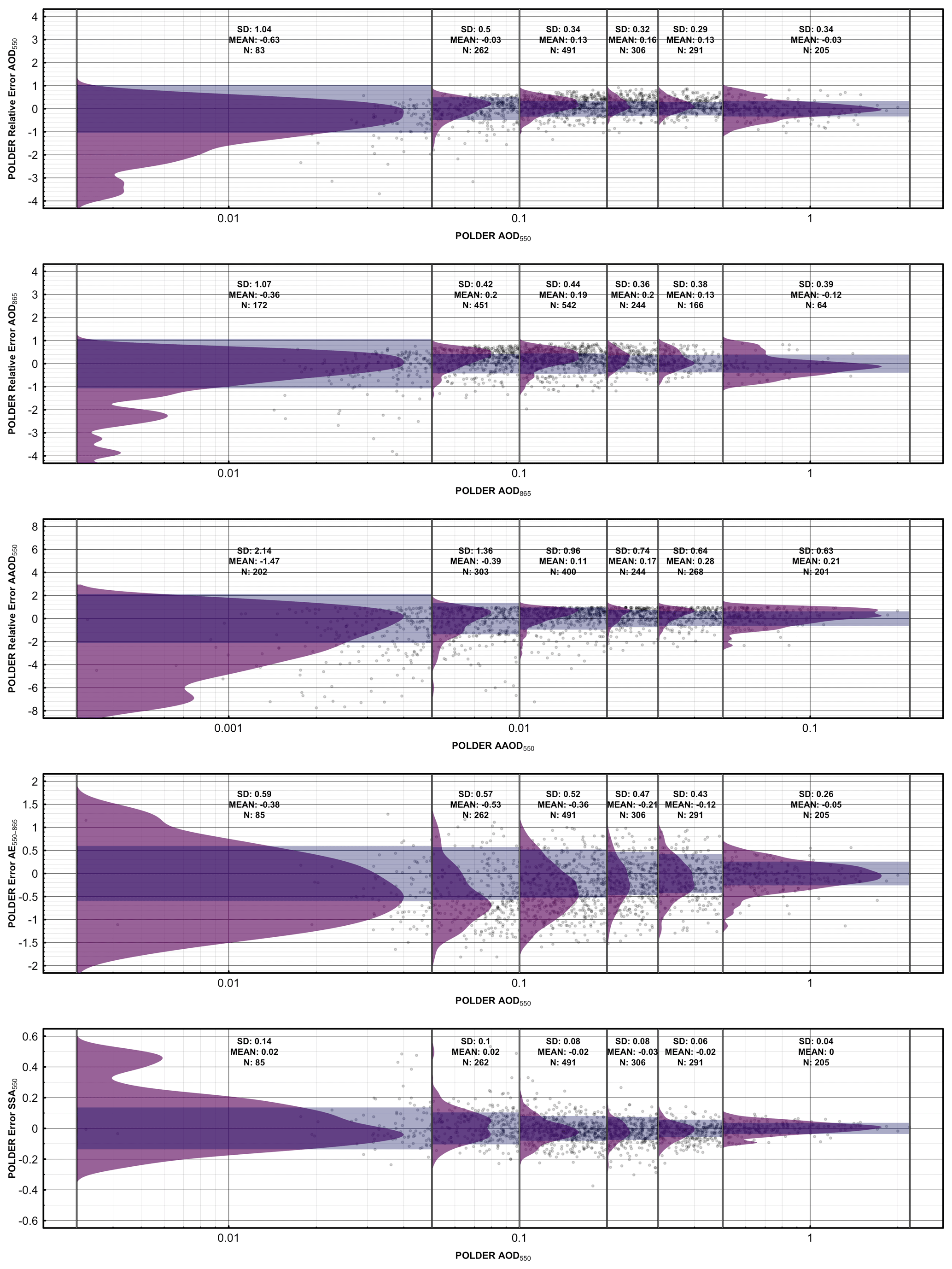
Figure A1 POLDER AOD₅₅₀, AOD₈₆₅ and AAOD₅₅₀ uncertainty estimation using the relative errors of POLDER – AERONET and POLDER AE_550−865 and SSA₅₅₀ uncertainty estimation using the differences of POLDER – AERONET. Each variable is partitioned in six bins along the XX' axis. The grey shade indicates the SD and the purple shade illustrates the distribution for each bin.

Appendix B

$$\begin{array}{}\text{(B1)}& {\displaystyle }\text{ME}={\displaystyle \frac{\mathrm{1}}{N}}\sum _i{\text{sim}}_i-{\text{obs}}_i\text{(B2)}& {\displaystyle }\text{MAE}={\displaystyle \frac{\mathrm{1}}{N}}\sum _i\left|{\text{sim}}_i-{\text{obs}}_i\right|\text{(B3)}& {\displaystyle }\text{RMSE}=\sqrt{\stackrel{\mathrm{‾}}{({\text{sim}}_i-{\text{obs}}_i{)}^{\mathrm{2}}}},\end{array}$$

where sim and obs are the simulated and observed values, while N is the population.