the Creative Commons Attribution 4.0 License.
the Creative Commons Attribution 4.0 License.
 | 19 Feb 2021
Comparison of chemical lateral boundary conditions for air quality predictions over the contiguous United States during pollutant intrusion events
Huisheng Bian
Zhining Tao
Luke D. Oman
Daniel Tong
Pius Lee
Patrick C. Campbell
Barry Baker
Cheng-Hsuan Lu
Jun Wang
Jeffery McQueen
Ivanka Stajner
The National Air Quality Forecast Capability (NAQFC) operated in the US National Oceanic and Atmospheric Administration (NOAA) provides the operational forecast guidance for ozone and fine particulate matter with aerodynamic diameters less than 2.5 µm (PM2.5) over the contiguous 48 US states (CONUS) using the Community Multi-scale Air Quality (CMAQ) model. The existing NAQFC uses climatological chemical lateral boundary conditions (CLBCs), which cannot capture pollutant intrusion events originating outside of the model domain. In this study, we developed a model framework to use dynamic CLBCs from the Goddard Earth Observing System Model, version 5 (GEOS) to drive NAQFC. A mapping of the GEOS chemical species to CMAQ's CB05–AERO6 (Carbon Bond 5; version 6 of the aerosol module) species was developed. The utilization of the GEOS dynamic CLBCs in NAQFC showed the best overall performance in simulating the surface observations during the Saharan dust intrusion and Canadian wildfire events in summer 2015. The simulated PM2.5 was improved from 0.18 to 0.37, and the mean bias was reduced from −6.74 to −2.96 µg m−3 over CONUS. Although the effect of CLBCs on the PM2.5 correlation was mainly near the inflow boundary, its impact on the background concentrations reached further inside the domain. The CLBCs could affect background ozone concentrations through the inflows of ozone itself and its precursors, such as CO. It was further found that the aerosol optical thickness (AOT) from satellite retrievals correlated well with the column CO and elemental carbon from GEOS. The satellite-derived AOT CLBCs generally improved the model performance for the wildfire intrusion events during a summer 2018 case study and demonstrated how satellite observations of atmospheric composition could be used as an alternative method to capture the air quality effects of intrusions when the CLBCs of global models, such as GEOS CLBCs, are not available.
- Article
(27982 KB) - Full-text XML
-
Supplement
(809 KB) - BibTeX
- EndNote


The chemical lateral boundary conditions (CLBCs) are pivotal to the prediction accuracy of regional chemical transport models (CTMs) (Tang et al., 2007, 2009). The CLBCs represent the spatiotemporal distribution of species concentrations along the lateral boundaries of the domain of a regional model. CLBCs can be either static or dynamic in type and can significantly affect CTMs predictions. One effect is imposing a constraint with static background concentrations for long-lived pollutants, such as CO and O3, which is the typical role of climatological CLBCs for non-intrusion events. For example, regional models like the Community Air Quality Multi-scale Model (CMAQ) hemispheric version (Mathur et al., 2017) utilizes static CLBCs that constrain chemical concentrations along the Equator. The influences of external pollutant intrusion events can only be achieved with dynamic (time-varying) CLBCs. Such CLBCs can come from a global model, a regional model that uses a larger domain (Tang et al., 2007), or observed profiles (Tang et al., 2009). Henderson et al. (2014) compiled a 10-year CLBCs database over the contiguous United States (CONUS) using a global chemical transport model (GEOS-Chem, Goddard Earth Observing System Model, Bey et al., 2001) and evaluated it against satellite-retrieved ozone and CO vertical profiles.
The US National Oceanic and Atmospheric Administration's (NOAA) National Air Quality Forecast Capability (NAQFC), which is currently based on the regional-scale CMAQ model, requires CLBCs for its daily prediction. The current NAQFC uses the dust-only aerosol CLBCs from the NOAA Environmental Modeling System (NEMS) Global Forecast System (GFS) Aerosol Component (NGAC) (Lu et al., 2016; Wang et al., 2018), which is an inline global model coupled with the Goddard Chemistry Aerosol Radiation and Transport (GOCART) aerosol mechanism (Chin et al., 2000, 2002; Colarco et al., 2010). Prior to the implementation of the NGAC CLBCs, NAQFC used the background, static aerosol profiles for the aerosol CLBCs (Lee et al., 2017). For the gaseous species, NAQFC uses modified monthly averaged CLBCs from a 2006 GEOS-Chem simulation (Pan et al., 2014). To alleviate surface ozone overpredictions, the upper-tropospheric ozone CLBCs from GEOS-Chem have been limited to ≤100 ppbv (parts per billion by volume).
Static CLBCs cannot capture the signals of some intrusion events, such as the biomass burning plumes from the outside of the domain, which could affect the prediction of ozone and particulate matter with aerodynamic diameter less than 2.5 µm (PM2.5). For non-intrusion events, Tang et al. (2007) investigated the sensitivity of regional CTMs to CLBCs and found that the background magnitude of the pollutant concentrations was more important than the variation of the CLBCs for the near-surface prediction over polluted areas. Over the contiguous USA, the northern and western USA are near to the prevailing inflow lateral boundaries where Canadian emissions and long-range transported Asian air masses can affect the chemical background concentrations. Additionally, the southern and eastern boundaries are subjected to the Saharan dust intrusions during the summer, which may result in surface PM2.5 concentration increases (Lu et al., 2016). CLBCs from global models are needed to fully assess such impacts of intrusion events and to advance the operational NAQFC. In this study, we extracted the CLBCs from the GEOS global chemical circulation model (Strode et al., 2019; Molod et al., 2012) in both static (monthly average) and dynamic (every 3 h) modes. The NAQFC runs using both GEOS and NGAC CLBCs are compared to a NAQFC base case with monthly 2006 GEOS-Chem CLBCs for summer 2015. During this period, the Canadian wildfires and Sahara dust storms affected the CONUS domain's northern and southern regions, respectively. In addition, we investigate the method of using satellite-derived CLBCs for pollutant intrusion events when CLBCs of global models may not be available.
The operational NAQFC is based on CMAQ version 5.0.2, driven by meteorological forecasts from NOAA and NCEP's (National Centers for Environmental Prediction) North American Mesoscale Model (NAM). The CMAQ configuration includes the CB05 (Carbon Bond 5) gaseous chemical mechanism (Yarwood et al., 2005) with updated toluene (Whitten et al., 2010) and chlorine chemistry (CB05tucl) (Tanaka et al., 2003; Sarwar et al., 2007) and AERO6 (Carlton et al., 2010; Foley et al., 2010; Sonntag et al., 2014), version 6 of the aerosol module, driven by NOAA and NCEP's North American Mesoscale Model (NAM) forecasting. It has a 12 km×12 km horizontal resolution covering CONUS, with 35 vertical layers up to 100 hPa. Anthropogenic area and mobile emissions are based on the on the 2011 US EPA (Environmental Protection Agency) National Emissions Inventory (NEI2011v2), and the point source emissions have been updated with the US EPA Continuous Emission Monitoring System (CEMS) for the prediction year (2015). Biogenic emissions are based on the Biogenic Emission Inventory System (BEIS) 3.14 (Pierce et al., 1998). Wildfire emissions originating inside the CONUS domain are estimated using the US Forest Service (USFS) BlueSky fire emissions estimation algorithm, in which the fire location information is provided by the NOAA Hazard Mapping System (HMS). The NOAA HMS is a satellite-based fire detection system that includes manual quality control. The detailed wildfire emission process of this system has been described in Pan et al. (2020).
Table 1The runs with different lateral boundary conditions (LBCs) conducted in this study. EC: elemental carbon; POC: primary organic carbon.
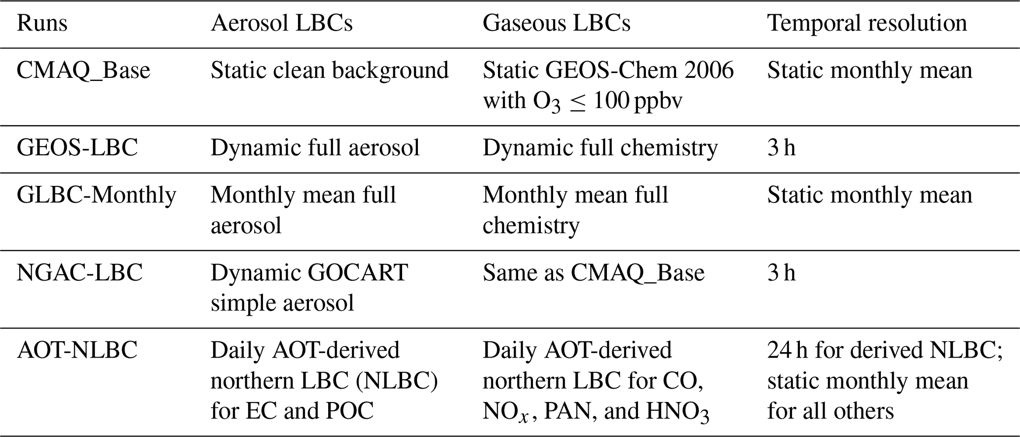
In this study, we conducted five model runs with different CLBCs (Table 1) over the CONUS domain (Fig. 1). The first run is the NAQFC–CMAQ base case (referred to as CMAQ_Base), which uses the modified GEOS-CHEM 2006 monthly gaseous CLBCs and clean aerosol background. The CMAQ_Base CLBCs were used in the earlier NAQFC system before NGAC was made available. The second run, NGAC-LBC, is the same as in CMAQ_Base for gaseous CLBCs but uses NGAC's dynamic aerosol CLBCs. The third run, the GEOS-LBC simulation, uses GEOS dynamic CLBCs and has full chemistry and dynamic variation for both gaseous and aerosol species, while the four-run GLBC-Monthly tests the GEOS monthly mean CLBCs to gauge the impacts of the CLBCs' temporal variability. The fifth and final run incorporates satellite-based aerosol optical thickness (AOT) for the northern CLBCs (AOT-NLBC). The AOT-NLBC run is the same as the GEOS-Monthly run, except that its northern boundary condition is generated from the relationship of VIIRS (Visible Infrared Imaging Radiometer Suite) AOT and GEOS-LBC for the wildfire intrusion events, which will be described later.
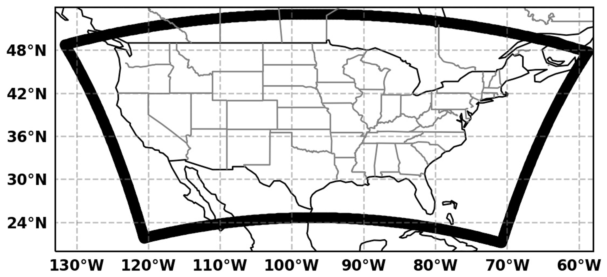
Figure 1NAQFC CONUS domain (outlined in bolded black). This figure is plotted using cartopy https://scitools.org.uk/cartopy/docs/latest/ (last access: February 2021), which uses the national and state border information from http://www.naturalearthdata.com/ (last access: February 2021). Please note that the above figure contains incomplete US state borders.
The extraction of the GEOS CLBCs for NAQFC's domain boundaries is based on the existing global-to-regional interface tool developed by Tang et al (2007, 2009) for MOZART (Model for Ozone and Related chemical Tracers), RAQMS (Realtime Air Quality Modeling System), and NGAC global models with additional enhancements to support GEOS's NetCDF4 format, vertical layers, and chemical species. This tool includes two major functions: spatial mapping and species mapping. Spatially, GEOS's concentrations from its 576×361 grid in a horizontal resolution with 72 vertical layers are three-dimensionally interpolated into CMAQ's CONUS lateral boundary periphery in a 12 km horizontal resolution. The species mapping is also needed due to the different chemical mechanisms employed in GEOS and CMAQ, as discussed in the following sections.
Table 2VOC (volatile organic compound) species mapping table from GEOS to CMAQ CB05tucl.
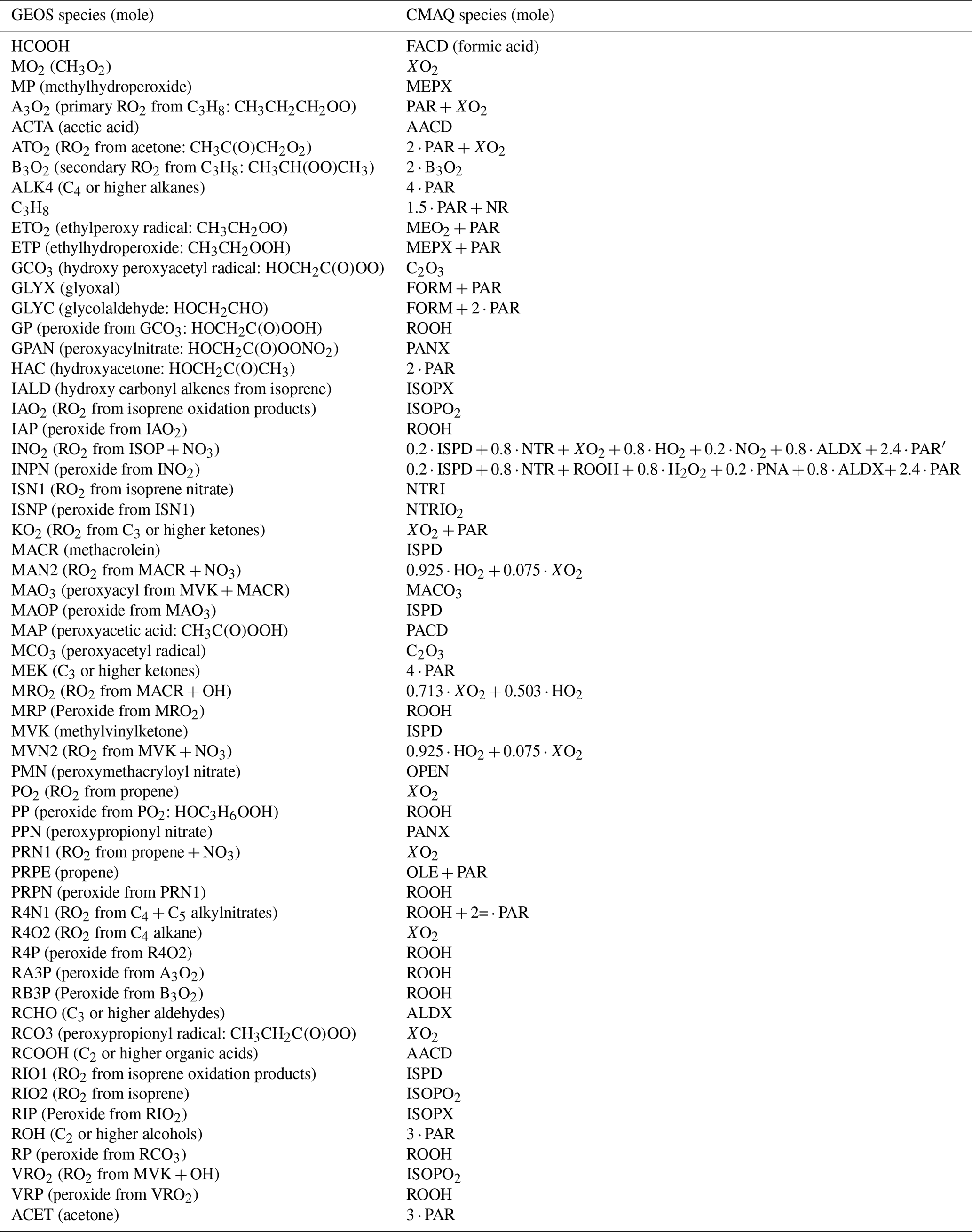
2.1 Gaseous species mapping
The GEOS outputs 122 gaseous chemical species and 15 aerosol species. For species such as O3, CO, NO, and NO2, an explicit one-to-one mapping can be achieved. However, some volatile organic compounds (VOCs) need special treatment during the conversions, as GEOS uses different lumping approaches compared to what is done in CMAQ CB05tucl (Carbon Bond 5 mechanism with toluene and chloride species). Table 2 lists the VOC species mapping used to convert GEOS's gaseous species to CMAQ's CB05tucl species. Two methods were employed for mapping the VOC species: one was based on the carbon bond structure, e.g., ALK4 → 4 PAR (Table 2), and the other was based on the similarity of the reactions. In GEOS, for example, the products of the isoprene reaction with NO3 are lumped into INO2, an intermediate RO2 radical.
The radical INO2 participates in the following reactions (Eastham et al., 2014; Tyndall et al., 2001):
The CB05tucl mechanism skips the intermediate INO2 and directly represents it as
Therefore, the GEOS INO2 species is split into seven CB05tucl species with the corresponding factors, respectively (Table 2). This conversion is just an approximation, and a perfect consistency for mapping these species can not be achieved due to the large differences between these two mechanisms, especially in regards to the complexity of isoprene chemistry. Fortunately, for the CONUS domain, the isoprene chemistry influence on the CONUS CLBCs are less significant when compared to the major intrusion events from wildfire plumes and dust storms. Most biogenically emitted species are short-lived, and their direct impact on CLBCs is relatively weak. A similar situation can also be applied to other short-lived species, such as NOx, which will be discussed later. Biogenic emissions can affect local photochemical processes, however, and subsequently generate relatively long-lived species, such as ozone and NTR. Such species may originate from outside the regional domain and thus have impacts on CLBCs and downstream chemistry. This issue is mitigated by the fact that most of these secondary long-lived species are explicitly included in both GEOS and CMAQ chemical mechanisms and can be directly mapped.
Other gaseous species are represented explicitly in the GEOS model, such as methylvinylketone (MVK), which is lumped in the CB05tucl's isoprene product (ISPD). In GEOS, the MVK mainly comes from isoprene, which is consistent with the CMAQ's ISPD source. Some GEOS species can also be mapped to CB05tucl species based on their carbon bonds, e.g., R4N2 (GEOS's C4−5 alkyl nitrates), which can be mapped to NTR + 2.0 PAR in the CB05tucl mechanism. Some of the mapping treatments, such as the ALK4 (C4 or higher alkanes) conversion to four paraffin carbon bonds (Table 2), may have a “truncation error”, as it only counted butane isomers. The effect of this truncation error, however, is likely relatively minor for CONUS CLBCs. The GEOS global model also mainly treats ALK4 as butane or Cn, where n∼4. Although GEOS's ALK4 emission includes some C5 or higher () alkanes, the relatively shorter lifetime of alkanes (Helmig et al., 2014) makes them harder to reach CONUS from their major upstream sources, such as East Asia. In this study, wildfire emissions may contribute to the alkane's impacts on the CONUS CLBCs, but these emissions are at least 1 order of magnitude lower than the corresponding wildfire CO, ethane, and propane emissions (Urbanski et al., 2008). Moreover, the impacts of the complex chemistry mapping on the CLBCs for the pollutant intrusion events (mainly wildfire events) are not expected to be significant for the ozone and PM2.5 predictions in this study, since the constituents of the major wildfire intrusion from the GEOS global model are CO, NOx, ethane, propane, elemental carbon (EC), and organic carbon (OC).
2.2 Aerosol species mapping
The GEOS model uses an updated GOCART aerosol scheme (Bian et al., 2017), compared to NGAC GOCART (Colarco et al., 2010, respectively), which includes additional species of ammonium and nitrates in three size bins (NO3an1, NO3an2, and NO3an3). Table 3 lists the aerosol species mapping from GEOS aerosols to CMAQ AERO6 species used in this study. GEOS aerosols have fixed size bins defined by their diameters, while CMAQ aerosols use three size modes, Aitken (ATKN), accumulations (ACC), and coarse (COR), or alternatively i, j, and k modes, respectively (Appel et al., 2010). Each of these size modes has its own lognormal size distribution (Whitby and McMurry, 1997). To convert the aerosol species from GEOS to CMAQ's AERO6, we need to consider not only the aerosol composition and the GEOS size bins conversion to the CMAQ size modes but also the size distribution within each CMAQ size mode that is controlled by the CMAQ aerosol number concentrations (the third column of Table 3). GEOS's dust aerosols are mapped to AOTHRJ (other unreactive aerosols in the accumulation mode) and ASOIL (soil particles in the coarse mode) in CMAQ. Although the CMAQ AERO6 has explicit elemental ions such as Ca and Mg, which are possible dust ingredients, we do not consider the reaction effects due to these ions. Tang et al. (2004) studied the dust outflow during the ACE-Asia (Asian Pacific Regional Aerosol Characterization Experiment) field experiment and found that only a small portion of cations in dust particles was available for aerosol uptake and reactions and that this portion is negligible for aged dust air masses.
Table 3Aerosol species mapping table from GEOS to CMAQ AERO6 (“D” represents the diameter of the GEOS aerosol bin).

During summer 2015, two intrusion events occurred, one in the southeastern USA and one in the northern USA, respectively. The southeastern intrusion was due to the long-range transported-dust storm from the Sahara. The northern intrusion was due to a Canadian wildfire event and its southward transport into the United States. Figure 2 shows the Suomi NPP (National Polar-orbiting Partnership) satellite's VIIRS AOT retrieval from later June to early July in 2015 and highlights these two intrusion events.
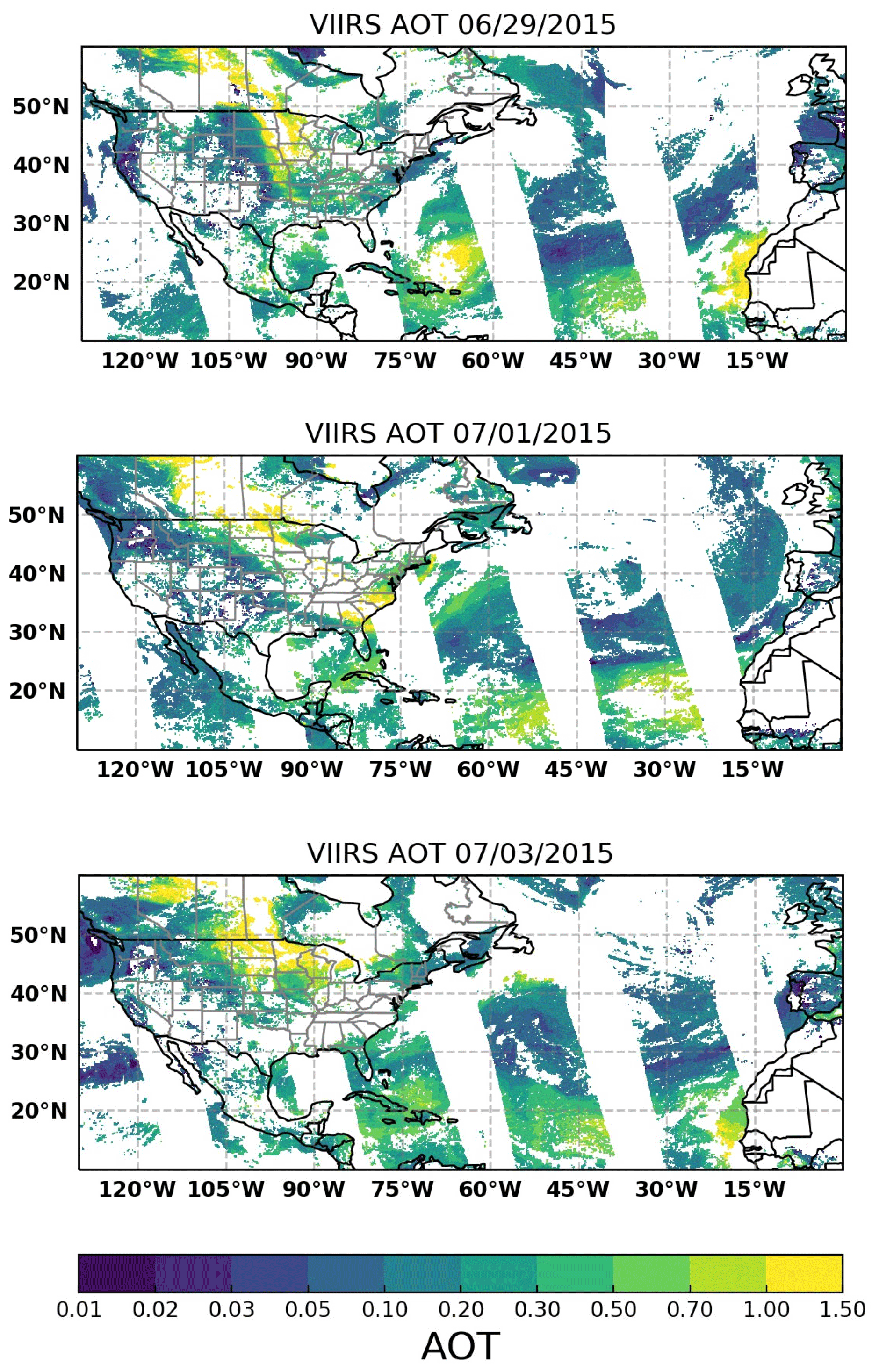
Figure 2Suomi NPP VIIRS aerosol optical thickness (AOT) on 29 June, 1 July, and 3 July 2015. Please note that the dates in this figure are given in the format of month day year (mm/dd/yyyy). This figure is plotted using cartopy https://scitools.org.uk/cartopy/docs/latest/ (last access: February 2021), which uses the national and state border information from http://www.naturalearthdata.com/ (last access: February 2021). Please note that the above figure contains incomplete US state borders and disputed territories.
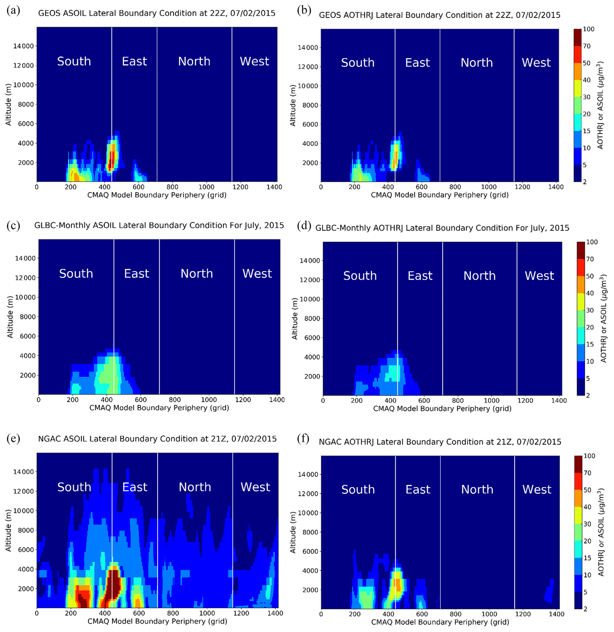
Figure 3The lateral boundary conditions for ASOIL (a, c, e) and AOTHRJ (b, d, f) along the domain periphery for 2 July 2015. The CMAQ LBC's grid index for each LBC segment is always from south to north and then from west to east, so the LBC index's start points are reset instead of being continuous for the north and west boundaries. Please note that the dates in this figure are given in the format of month day year (mm/dd/yyyy).
3.1 Dust storm events in summer 2015
As shown in Fig. 2, a dust storm originating from the Sahara reached the southeastern USA via transatlantic transport. The two global models, GEOS and NGAC, captured this dust intrusion and increased the aerosol CLBCs of NAQFC. Figure 3 shows the corresponding three CLBCs for ASOIL and AOTHRJ along the model's boundaries on 2 July 2015. With the exception of CMAQ_Base, all the other three CLBCs showed enhanced ASOIL (the coarse-mode dust) and AOTHRJ (the accumulation-mode dust) near the domain's southeastern corner and the south-central boundary. GLBC-Monthly represents the monthly average of GEOS-LBC for July 2015 and has the lowest increments for the two types of aerosols. The two dynamic CLBCs, GEOS-LBC and NGAC-LBC, showed similar aerosol increments along the domain boundaries. However, the NGAC aerosols tended to have a broader spread than those of GEOS-LBC, especially for ASOIL, which could reach above an altitude of 10 km with concentrations greater than 5 µg m−3 (Fig. 3e). NGAC-LBC also showed enhanced dust signals over the western boundary, where GEOS-LBC did not show any dust-related aerosols. Another difference between these two CLBCs was their ratio of AOTHRJ versus ASOIL. The dynamic NGAC-LBC had higher ASOIL, the coarse-mode dust, than that of GEOS-LBC (Fig. 3a and e), but its AOTHRJ was lower than the latter (Fig. 3b and f). This is particularly true over the south-central boundary, where GEOS-LBC had AOTHRJ up to 30 µg m−3. It implies that besides their difference in transport patterns, these two global models also had some differences in their dust size distributions.

Figure 4Model-predicted surface PM2.5 concentrations with the four LBCs on 2 July 2015 (the colored circles showing the AIRNow observations). Please note that the dates in this figure are given in the format of month day year (mm/dd/yyyy).
Figure 4 shows comparisons of the simulated PM2.5 concentrations against the observations from the US EPA AIRNow stations. CMAQ_Base represented a clear background situation and has obviously missed this dust intrusion event and underestimated the PM2.5 over the southern and southeastern United States. The two dynamical CLBCs, GEOS-LBC and NGAC-LBC, captured the intrusion signals well and yielded the best model performance. While both GEOS-LBC and NGAC-LBC underpredicted PM2.5 over central Florida, their performance was improved compared to CMAQ_Base. Further downwind over Texas, GEOS-LBC yielded more widespread and higher PM2.5 enhancements compared to NGAC-LBC and agreed better with the observations (except for the overpredictions over northern Texas). GLBC-Monthly run had a moderate PM2.5 enhancement but still underestimated the dust intrusion, falling between CMAQ_Base and two dynamic CLBC cases in magnitude of PM2.5 enhancements. Figure 5 shows a similar story for the scenario of 3 d later. GEOS-LBC yielded the best overall model performance, although it still underpredicted the PM2.5 concentration over Florida and northern Texas.
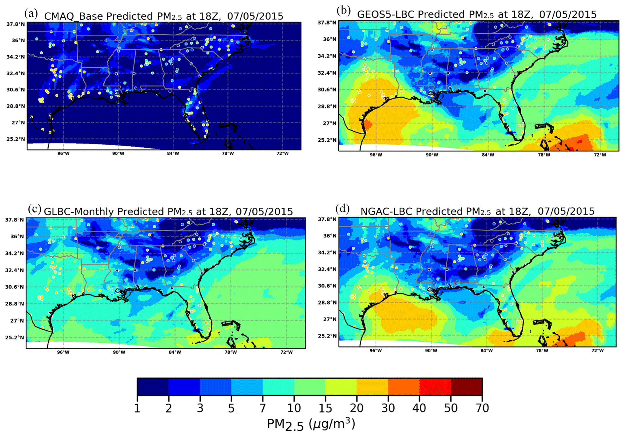
Figure 5Same as Fig. 4 but for 5 July 2015. Please note that the dates in this figure are given in the format of month day year (mm/dd/yyyy).
A time-series comparison over Florida and Texas showed that, in general, the best models regarding performance in capturing the dust intrusion are, in order, GEOS-LBC, NGAC-LBC, GLBC-Monthly, and CMAQ_Base (Fig. 6). An exception, however, is NGAC-LBC's underprediction for PM2.5 concentrations over Florida in June. These comparisons demonstrate the advantage of using dynamic CLBCs for capturing intrusion events. The dynamic CLBCs (GEOS-LBC and NGAC-LBC) still missed some intrusion peaks, such as the one on 30 June over Texas, and also showed disagreement with the observed temporal variability, e.g., 1 July over Florida and 8 July over Texas. It should be noted that the nighttime PM2.5 spike on 4 July (5 July in UTC) was not related to the dust intrusion but was caused by US Independence Day's fireworks. This firework emission was not included in our anthropogenic emission inventory. Most firework emissions were injected in elevated levels, and the associated pollutants could be transported to extended downstream areas. If the downstream areas were relatively big, its regional averaged effect could appear for a longer time. This is the reason why some PM2.5 concentration spikes that started on 4 July could last longer than the firework emission durations, e.g., 1 h.
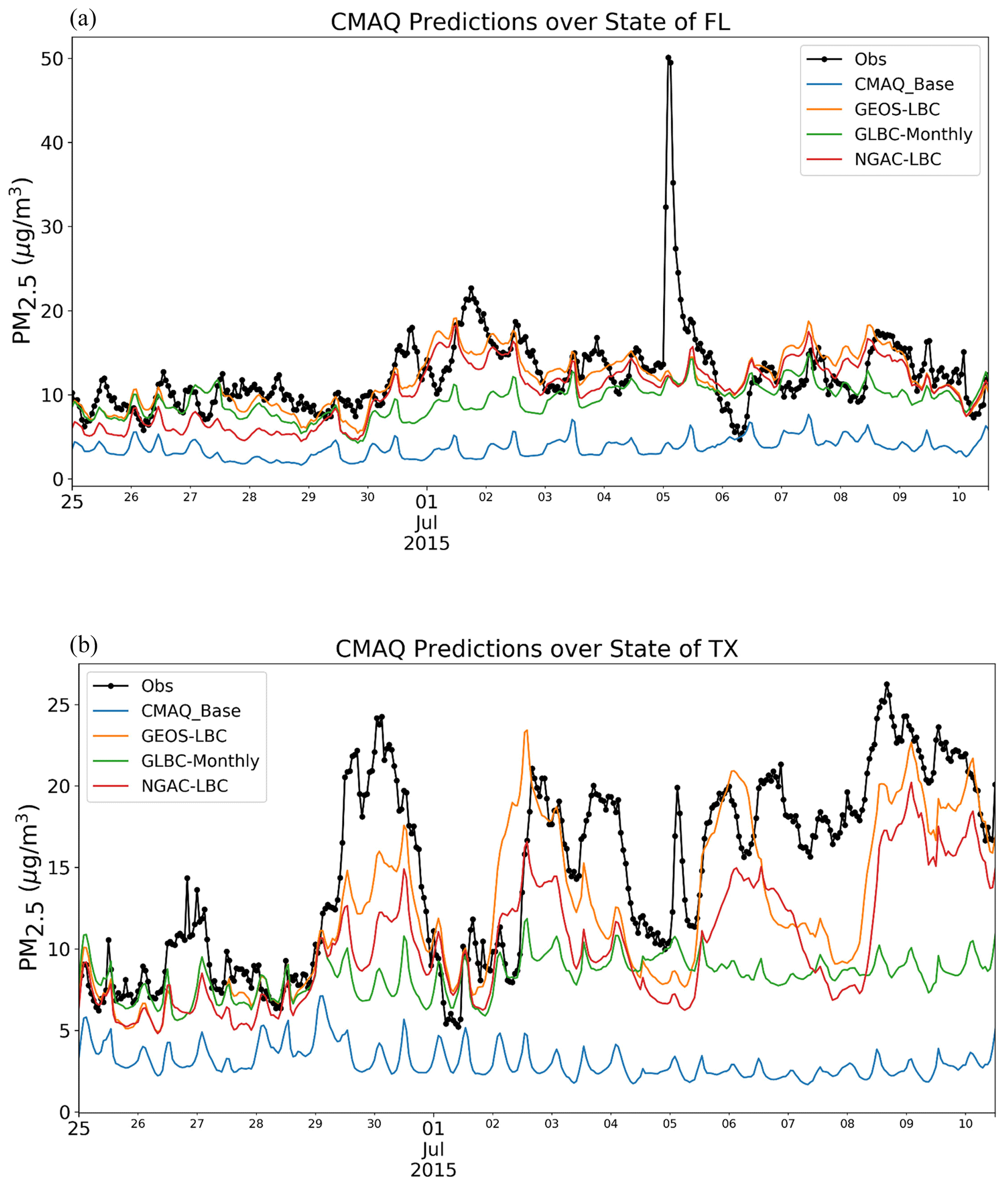
Figure 6Time-series PM2.5 comparisons over the states of Florida (FL) and Texas (TX). All the times are in UTC.
3.2 The wildfire event in summer 2015
During the same period of summer 2015, a wildfire event occurred in Canada, and the biomass burning plume was transported to the northern USA, as shown in Fig. 2. While the dust storm intrusions mainly affected the aerosol concentrations, the biomass burning plumes also included gaseous pollutants, such as enhanced levels of CO, NOx, and VOCs, which could affect the photochemical generation of ozone. For aerosol species, the biomass burning air mass mainly consisted of elemental carbon (EC) and primary organic carbon (POC), which are associated with AECJ+APOCJ in CMAQ (Table 3). GEOS-LBC showed the highest aerosol and CO concentrations with AECJ + APOCJ up to 300 µg m−3 and CO up to 3000 ppbv along the domains northern boundary (Fig. 7). It also showed CO enhancement at elevated altitudes up to 12 km (Fig. 7b). The monthly averaged CLBCs, GLBC-Monthly, had patterns similar to GEOS-LBC but with much lower concentrations (Fig. 7c and d). NGAC-LBC had similar AECJ + APOCJ profiles to those of GLBC-Monthly, but its static CO boundary condition (same as CMAQ_Base) did not reflect the wildfire influence (Fig. 7e and f).
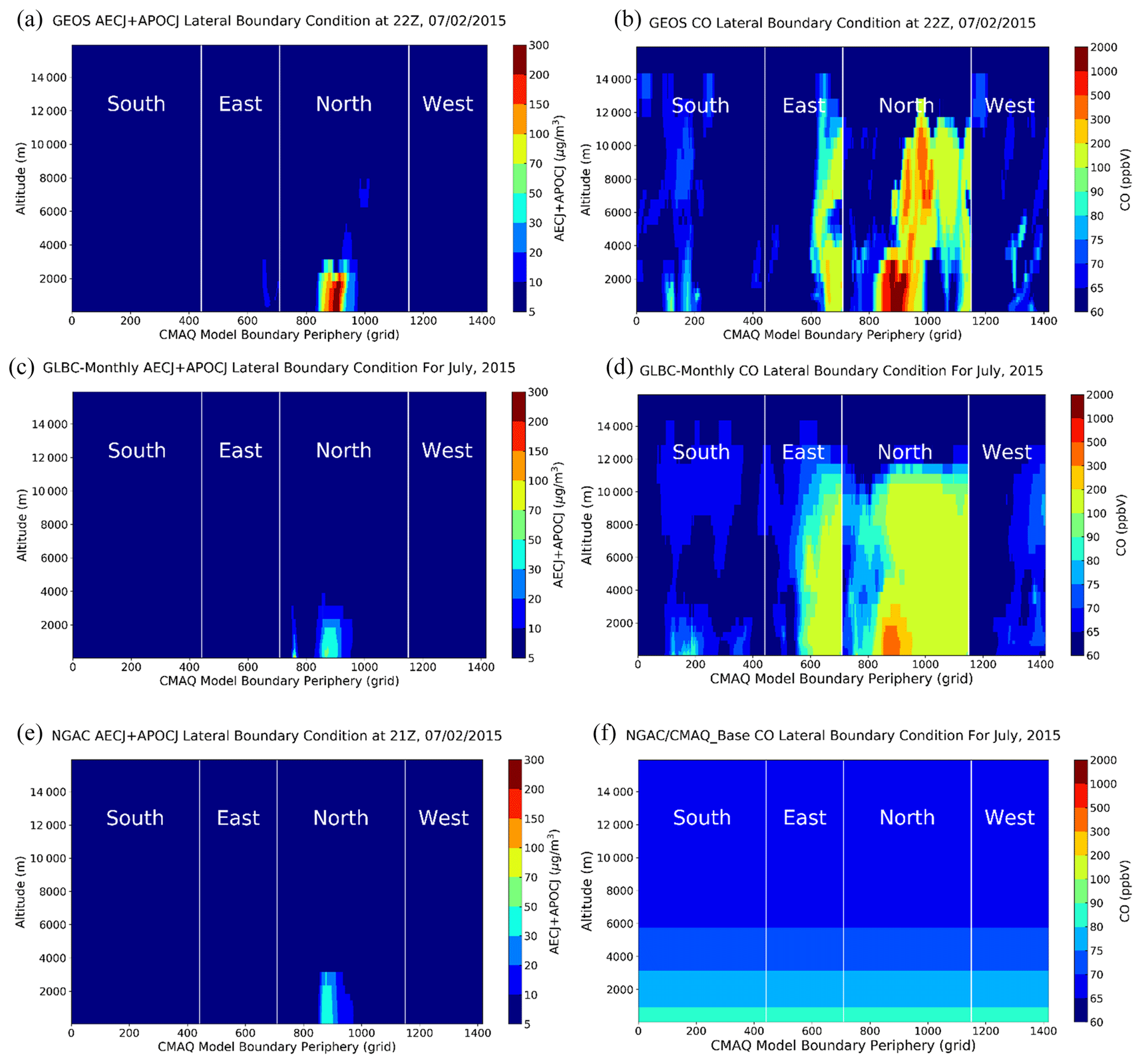
Figure 7Same as Fig. 3 except for total EC and POC (AECJ + APOCJ) (a, c, e) and CO (b, d, f). Please note that the dates in this figure are given in the format of month day year (mm/dd/yyyy).
The enhanced gaseous pollutants in the full-chemistry CLBCs increased the photochemical generation of ozone, and consequently the higher ozone appeared along the north-central boundary (Fig. S1a and b in the Supplement), where GEOS-LBC showed 10 ppbv or higher O3 concentrations compared to the static NGAC-LBC and CMAQ_Base for the altitudes of < 4 km (Fig. S1c). The wildfire-induced ozone enhancements appeared not only in the lower troposphere but also at higher altitudes, e.g., 11 km, and were not solely due to downward transport of high stratospheric ozone (Fig. S1a). The full-chemistry GEOS-LBC also indicated that the short-lived NOx had less than a 1 ppbv increase (Fig. S2a) due to the wildfire intrusion. The NOz (sum total of all NOx oxidation products, NOz = NOy − NOx) enhancements, however, could reach 30 ppbv (Fig. S2b) along the northern boundary around 10–12 km altitude and co-existed with the CO increments (Fig. 7b). NOz is a good indicator for the photochemical formation of ozone (Sillman et al., 1997), while the ratio represents the ozone photochemical efficiency per NOx. The high-altitude CO and NOz increments reflected that the GEOS model had strong fire plume rise and injected wildfire emissions into the upper troposphere. The VOCs also showed increments due to the wildfire, which mainly provided the VOC- and CO-rich air mass with limited NOx to the regional CMAQ model. When this CO- and VOC-rich air mass arrived at NOx-rich regions, such as the urban areas, it could contribute to the photochemical generation of ozone.
Figure 8 shows the comparison of PM2.5 predictions on 3 July 2015 at 18:00 UTC. CMAQ_Base missed the intruded biomass burning plumes and the corresponding high PM2.5 over North Dakota, South Dakota, Montana, and Minnesota (Fig. 8a). GEOS-LBC predicted the highest PM2.5 increment (up to 200 µg m−3) over these states and agreed best with the AIRNow observations (Fig. 8b). The dynamic NGAC-LBC and static GLBC-Monthly showed similar PM2.5 enhancements over the affected states but were almost 1 order of magnitude lower than that of GEOS-LBC.
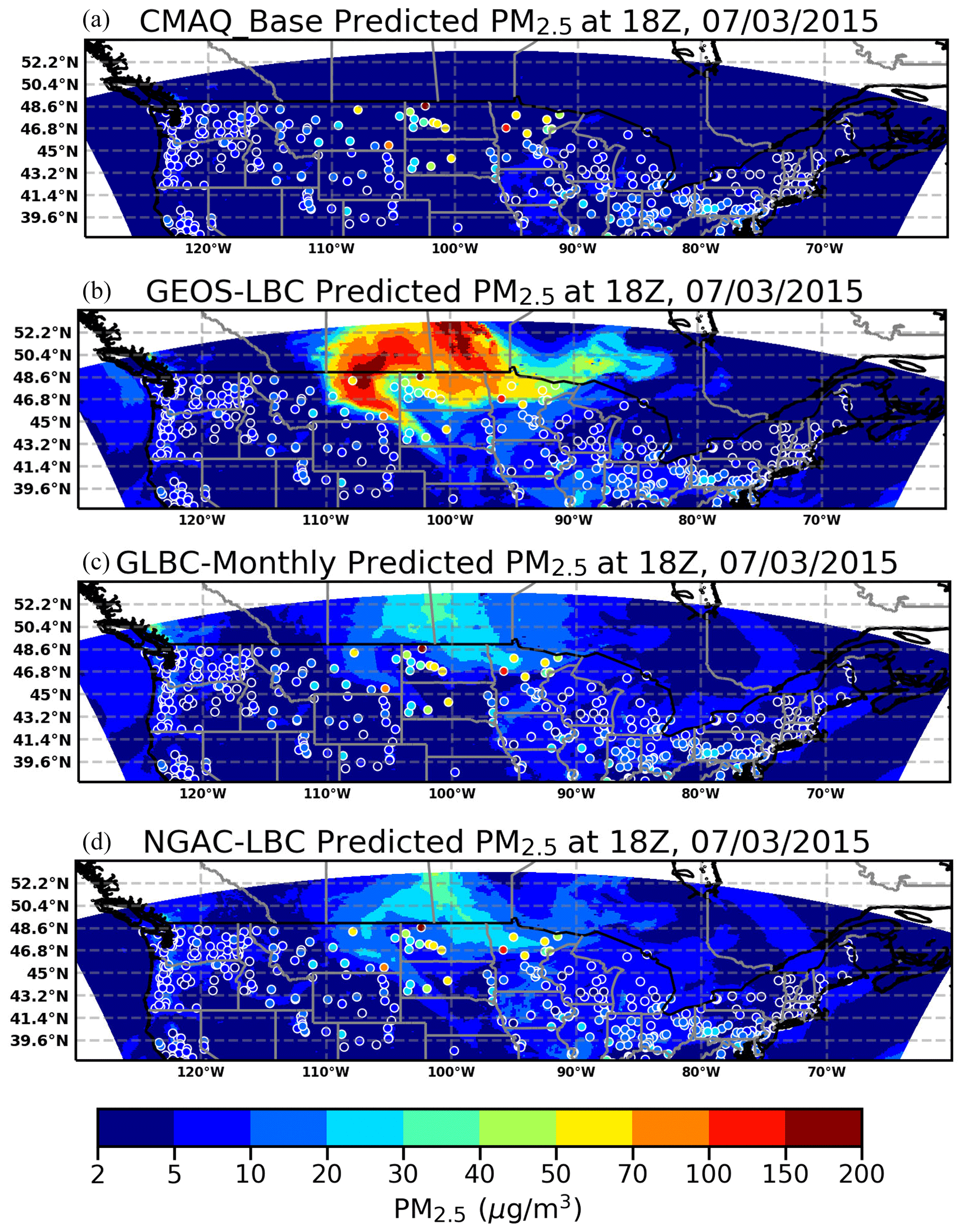
Figure 8Same as Fig. 4 but for the northern USA on 3 July 2015. Please note that the dates in this figure are given in the format of month day year (mm/dd/yyyy). This figure is plotted using cartopy https://scitools.org.uk/cartopy/docs/latest/ (last access: February 2021), which uses the national and state border information from http://www.naturalearthdata.com/ (last access: February 2021). Please note that the above figure contains incomplete US state borders.
Figure 9 shows similar predictions but for ozone, where GEOS-LBC yielded the highest ozone increase due to the wildfire plume but still underestimated the ozone over North Dakota (Fig. 9b). GLBC-Monthly systematically underestimated the ozone over all of these regions. CMAQ_Base and NGAC-LBC used the same static gaseous CLBCs, including that for ozone, and gave even larger underestimates. NGAC-LBC had more wildfire-induced aerosol loading and consequently a lower photolysis rate compared to CMAQ_Base. As both NGAC-LBC and CMAQ_Base had the “cleaner” air mass with low concentrations of ozone precursors over the northern USA, the photolysis reduction due to aerosols mainly led to the reduced ozone photolytic destruction, such as O3 →O1D + O2 or O3 → O3P + O2, instead of its photochemical generation. For the same reason, ozone's lifetime in winter is longer that in summer (Janach, 1989). Over polluted regions, however, the photolysis reduction would cause a lower ozone concentration by limiting its photochemical production. Overall, this effect of photolysis rates on ozone was relatively small.
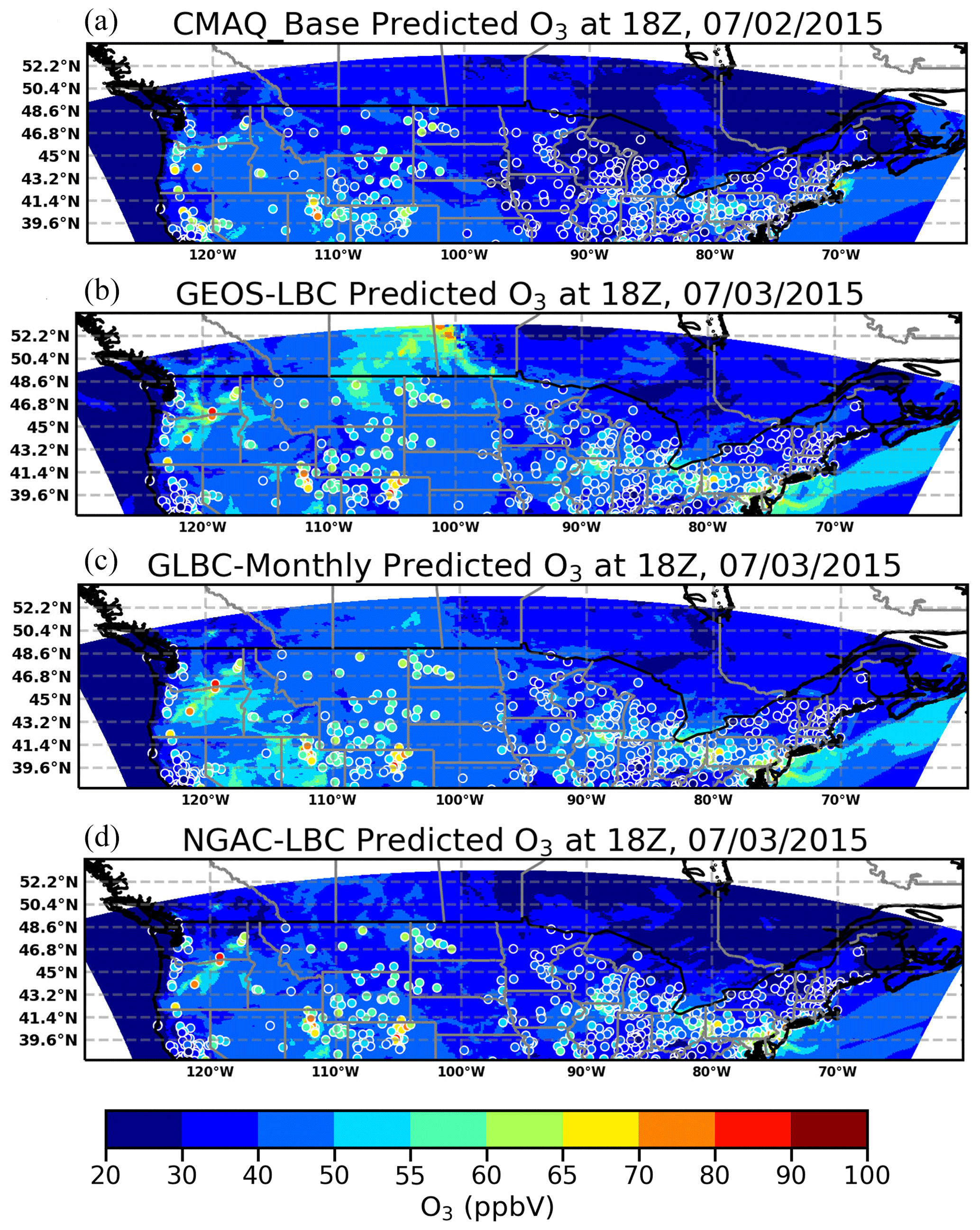
Figure 9Same as Fig. 8 but for O3. Please note that the dates in this figure are given in the format of month day year (mm/dd/yyyy). This figure is plotted using cartopy https://scitools.org.uk/cartopy/docs/latest/ (last access: February 2021), which uses the national and state border information from http://www.naturalearthdata.com/ (last access: February 2021). Please note that the above figure contains incomplete US state borders.
Figure 10 shows the time-series comparison over the north-central and northeastern USA for surface PM2.5 and ozone concentrations, in which GEOS-LBC showed better PM2.5 predictions compared to the other cases, especially from 29 June to 2 July over the northern USA. GEOS-LBC still had the systematic PM2.5 underestimation on the night of 4 July due to the missed firework emissions and underestimated PM2.5 further downwind in the northwestern USA. GEOS-LBC also better captured the peak ozone concentrations, e.g., 1 to 2 July, though it overpredicted ozone in some instances, especially during nighttime. The small ozone differences (regional averages of < 1 ppbv) between CMAQ_Base and NGAC-LBC reflected the impact of wildfire aerosols on the photolysis rates (Fig. 9c and d).
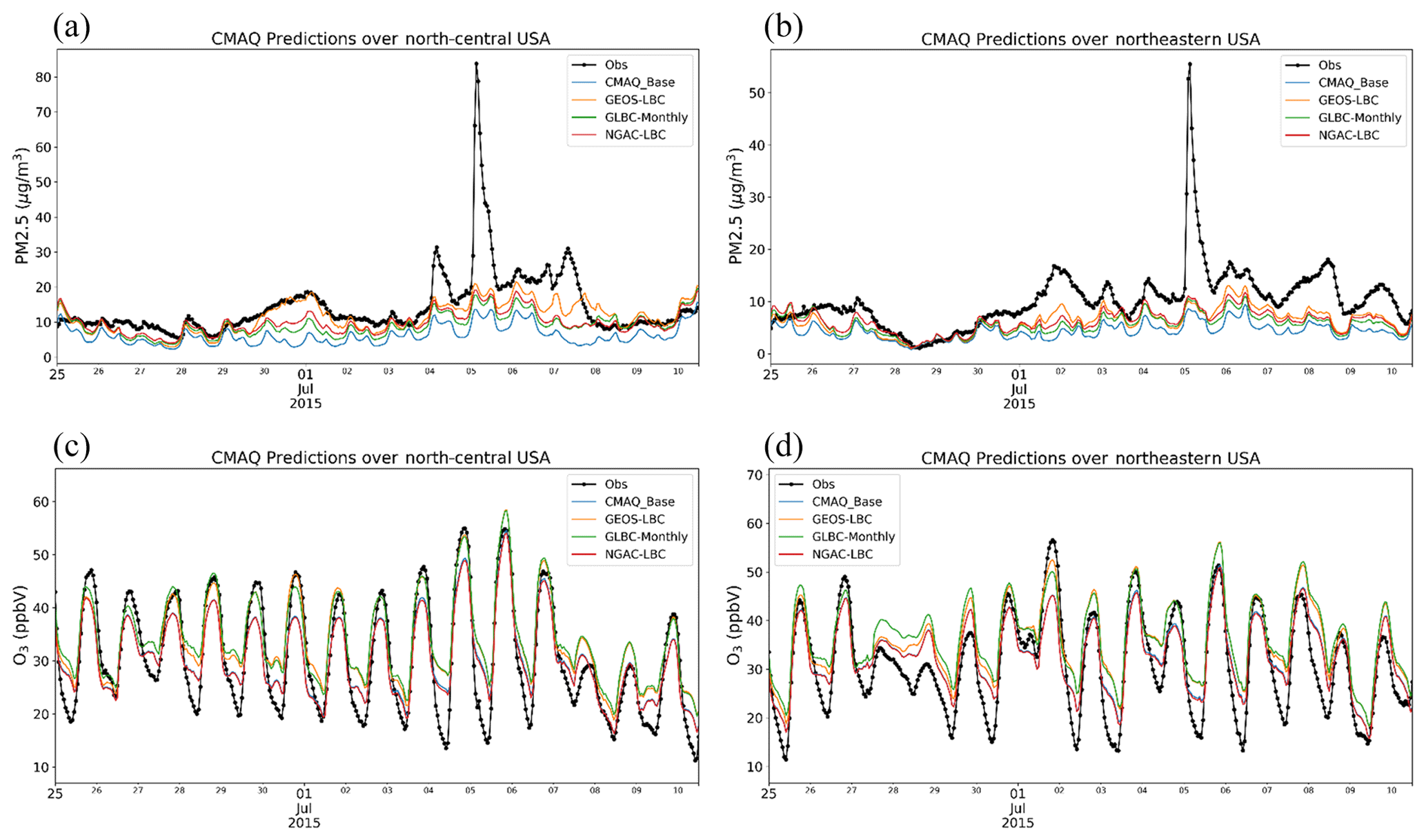
Figure 10Time-series comparisons for PM2.5 (a, b) and O3 (c, d) over the north-central region (a, c) (states of Illinois, Indiana, Iowa, Kentucky, Michigan, Minnesota, Missouri, Ohio, and Wisconsin) and northeastern USA (b, d) (states of Connecticut, Delaware, Maine, Maryland, Massachusetts, New Hampshire, New Jersey, New York, Pennsylvania, Rhode Island and Vermont and the District of Columbia).
3.3 Statistics and discussion
Table 4 summarizes the PM2.5 statistics during the 2 weeks of the intrusion events over the CONUS domain and sub-regions. The dynamic CLBCs, GEOS-LBC and NGAC-LBC, showed significant improvements for almost all scores over these regions as compared to CMAQ_Base. GLBC-Monthly was also better than the base case, though its correlation coefficient (R) and index of agreement (IOA) were lower than those of the dynamics CLBCs, as the time-averaging method removed the temporal variability. Over the further downwind regions of the intrusion events, the CLBCs' impact depended on the regional characteristics of the pollutant concentrations. For instance, since the Rocky Mountain region was relatively clean due to its low local PM emissions, the external influence weighed more, and thus the CLBCs showed more significant impact there. Over more polluted regions where relatively strong local PM emissions existed, such as the Pacific Coast and the northeastern USA, the CLBCs mainly changed the background concentration for PM2.5 and had a very limited impact on R or IOA. Overall, GEOS-LBC yielded the best scores in terms of mean bias (MB), root mean square error (RMSE), R, and IOA. The other dynamic CLBCs, NGAC-LBC, had the next best performance, and CMAQ_Base ranked last in terms of the PM2.5 prediction.
Table 4Regional PM2.5 statistics of the four simulations (CMAQ_Base, GEOS-LBC, GLBC-Monthly, and NGAC-LBC) from 24 June to 8 July 2015.
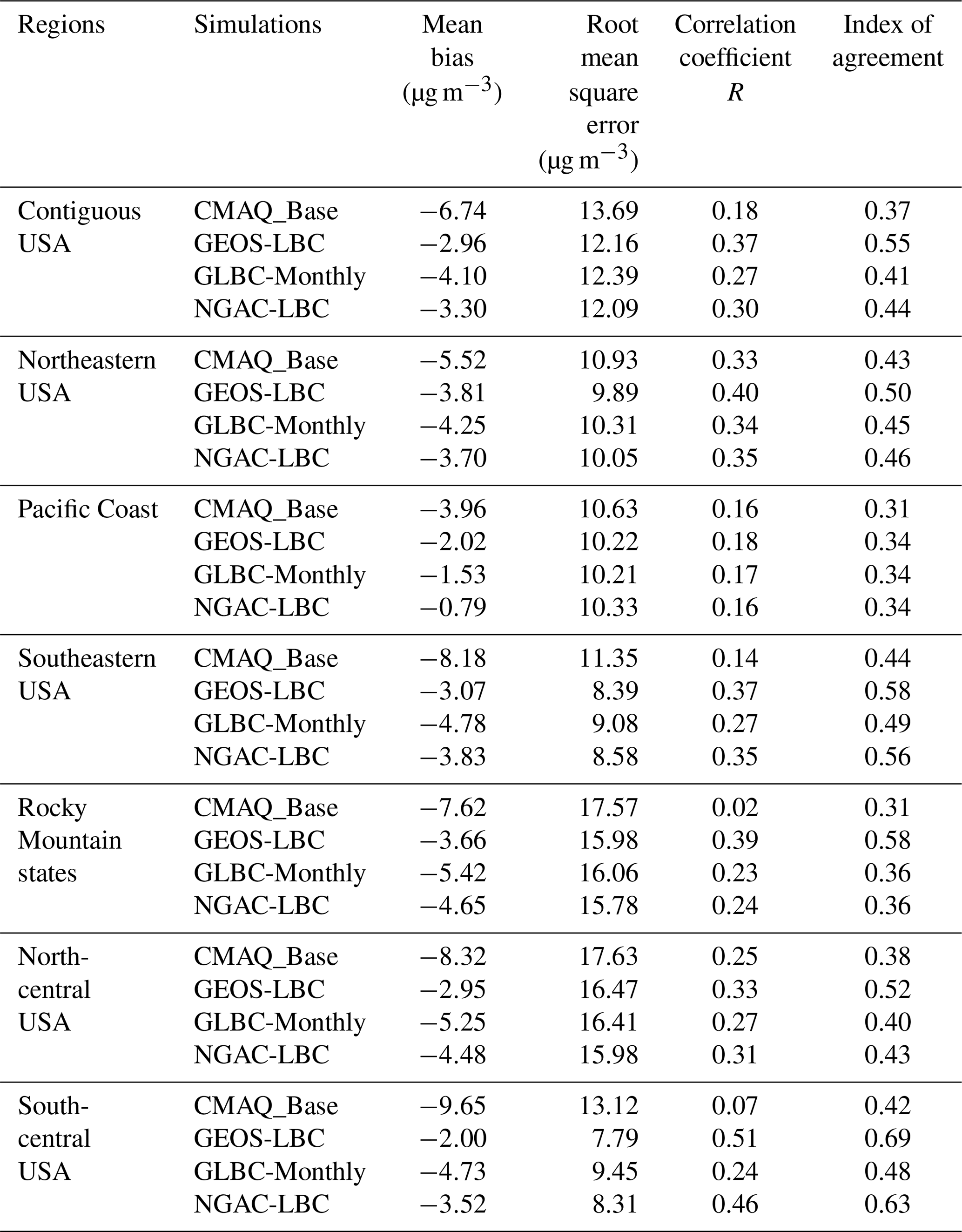
Table 5 shows the similar statistics for ozone. CMAQ_Base had a preexisting O3 overprediction, especially over the south-central USA, which affected the impacts of the CLBCs and the corresponding model performance changes. Differing from PM2.5, ozone had strong diurnal variation during the summertime, which resulted in relatively fewer impacts of the CLBCs on R and IOA. NGAC-LBC did not change any precursor concentrations related to ozone production and thus only affected the ozone formation by reducing photolysis rates. Therefore, as compared to CMAQ_Base, NGAC-LBC had very weak influence on O3 and only reduced the regional O3 by around 0.2 ppbv, with little to no impact on R or IOA. GEOS-LBC tended to increase ozone concentrations in most regions, except the south-central USA, where GEOS-LBC showed general improvement for all statistical metrics. GEOS-LBC had the weakest impact on ozone over the Pacific Coast and Rocky Mountain regions or the farther downstream areas. GLBC-Monthly had the largest ozone increase over most regions except the south-central region and also had the slightly higher RMSE. This result suggests that averaging the temporal variation of CLBCs may not have a linear effect on ozone predictions. GEOS-LBC showed the best model performance compared to other runs except the mean bias over most regions, though its improvement for O3 was not as significant as that for PM2.5. As discussed above, the CLBCs' impact on ozone inside the domain was realized through changing inflow concentration of the O3 inflow itself and/or O3 precursors, such as NOx, VOC, or CO. The distance or depth of the CLBCs' effective impact from the inflow boundary depended on the lifetime of these species. All these species have a longer lifetime in winter compared to summer. Our other study showed that the CLBCs' impact on ozone in winter was stronger than that in summer.

The GEOS-LBC case is further used to illustrates the impact of CLBCs on the prediction statistics and their relations to the distance from the domain boundary during the pollutant intrusion events across the southern (the Saharan dust storm, Fig. 11a and b) and the northern USA (wildfire, Fig. 11c and d). The CLBCs have two effects for the regional predictions: (1) they provide a constraint for background concentrations represented by the mean biases, and (2) they introduce a dynamic external influence, represented by the correlation coefficients. The CLBC impacts on the background and variability both affect the RMSE of predictions. Over the southern USA, the Saharan dust storm intruded through the states of Texas and Louisiana, 100 to 86 ∘W, and moved northward (Fig. 4). Figure 11a showed that GEOS-LBC's improvement on the correlation coefficient (R) for the PM2.5 prediction reached the highest near the southernmost near-boundary region and gradually reduced along the latitude for the inland region. On the other hand, the corresponding MB improvement for PM2.5 did not show a significant reduction along the distance from the influenced boundary. The second effect of CLBCs, which constrains PM2.5 background concentrations, can exist further inside of the domain. The PM2.5 RMSE change reflected the combined changes of the MB and R value. The improving impact of GEOS-LBC on the RMSE also became weaker moving from the boundary because the MB did not vary much and the RMSE changes followed the correlation coefficient's change northward. Contrary to PM2.5, the most significant R improvement for O3 was not near the boundary but rather for more northward regions (29 to 32∘ N) (Fig. 11b). Overall, for the dynamic CLBCs, the improvements in the ozone MB and RMSE have similar spatial variability, which is more significant near the inflow boundary and fades further inland.
Figure 11The latitudinal distributions of correlation coefficient R (black), mean bias (MB) (red), and root mean square error (RMSE) (blue) of PM2.5 (a, c) and O3 (b, d) concentrations from 24 June to 8 July 2015 over the southern USA (a, b) and northern USA (c, d) for CMAQ_Base (solid line) and GEOS-LBC (dash line) runs. Please note that the dates in this figure are given in the format of month day year (mm/dd/yyyy).
Differences in PM2.5 and O3 statistics arise because O3 typically has a stronger diurnal variation in summer driven by local photochemical activities in polluted regions, which may impact the correlation more than the external CLBCs. Therefore, GEOS-LBC's major influence on O3 prediction for this event was changing the O3 background concentration. The GEOS-LBC MB change for ozone was also variable compared to the CMAQ_Base case northward from the boundary (Fig. 11b). GEOS-LBC had a lower ozone concentration compared to CMAQ_Base at low altitudes for the southern boundary but had higher ozone concentrations in the altitudes higher than 14 km (Fig. S1). The high ozone concentration could reach the surface after a certain distance of downward transport in the model system with strong vertical mixing (Tang et al., 2009), which results in the higher ozone MB of GEOS-LBC over the deeper inland region.
There was a similar spatial distribution for the PM2.5 statistical differences between GEOS-LBC3 and CMAQ_Base for the wildfire intrusion event over the northern USA. The most significant R and RMSE improvements for GEOS-LBC appeared near the boundary, and these improvements were reduced farther from the boundary. However, the corresponding MB differences could exist deeper inland. For O3, the difference between the GEOS-LBC and CMAQ_Base cases became more complex because wildfire plumes also contained the intrusion from O3 and its precursors. The GEOS-LBC run generally yielded higher O3, which exacerbated the preexisting model overprediction near the boundary but helped reduce the ozone underpredictions further inland (Fig. 11d). The largest O3 MB differences were also farther away from the boundary itself, as it took more time for the for ozone precursors to contribute to the photochemical formation of O3. The spatial variation of the O3 RMSE difference was similar to that of the O3 MB except for the further inland region, such as south of 43∘ N, where GEOS-LBC did not improve the RMSE. A similar issue also appeared for the R difference for the region south of 46∘ N, implying that the intruded wildfire plume represented by GEOS-LBC could introduce some spatial or temporal biases for O3 precursors.
The dynamic CLBCs, such as GEOS-LBC, showed an overall better prediction of the pollutant intrusion events by better capturing the spatiotemporal impacts of external gases and aerosols across the domain of the regional model. However, the full-chemistry CLBCs sometimes are not easy to obtain, especially for a near-real-time forecast. Some event-dependent emissions, including wildfires, may need additional time to retrieve and refine and thus may lag behind the valid forecast times. In order to represent the intrusion influence when the real-time model CLBCs are not available, we test an alternative CLBC method based on the historical data adjusted with certain indicators. Here we focus on the wildfire intrusion, since it is more difficult to capture the sudden outbreak of wildfire signals than the long-range transported-dust intrusion. Further alleviating this issue for dust intrusion is the current availability of the operational NGAC dust forecasting for NAQFC (Wang et al., 2018).
4.1 Development of the CLBCs with VIIRS AOT for wildfire plumes
While ground-based AIRNow surface stations are reliable and could be a historical data indicator to represent intrusion events, their spatial coverage along the wildfire intrusion boundaries is not dense enough for this purpose. VIIRS AOT retrievals, however, well reflected the wildfire intrusion with broad spatial coverage, superior to the sporadic surface stations along the northern boundary of the CONUS domain (Fig. 2). Thus, VIIRS AOT may be used as an indicator for wildfire plumes. Figure S3 showed the comparison of extracted VIIRS AOT versus GEOS CO and EC column loading along the northern boundary for June to July 2015, with their correlation coefficients (R) of > 0.5. The regression relationship derived out of Fig. S3 can be used to resample the historical GEOS-LBC data to derive the new CLBCs for wildfire intrusion events when the corresponding AOT is available. This regression methodology is strengthened by the fact that the domain's northern boundary was relatively clean in most periods of the summer, unless the wildfire events occurred. During June and July 2015, the VIIRS AOT data were available once or twice per day around local noontime under cloud-free conditions. To maximize the amount of VIIRS AOT data used along the northern boundary, we relaxed the radius of influence up to 300 km when “nearest-neighbor” pairing of the VIIRS AOT geolocation and the northern boundary location. Here we paired the GEOS's northern CLBCs (NLBC) for 18:00 UTC with the daily VIIRS AOT along the same location and averaged the whole column with an AOT interval of 0.2 to build a CLBC database sorted in AOT. We only chose to resample the CLBCs for the primarily emitted species from the wildfire sources, which include POC, EC, CO, NOx, and two NOz species, PAN and HNO3, but did not include the ozone CLBCs. When VIIRS AOT data are available for a NLBC grid in new intrusion events, the whole-column species concentration data from that database are chosen to form the new CLBCs for that grid based on the nearest-neighbor VIIRS AOT value.
4.2 A case study with VIIRS-AOT-derived LBC in August 2018
In mid to late August 2018, there were dominant high-pressure and dry-weather conditions that led to a wildfire outbreak that quickly spread across western Canada (Fig. S4). There was prevailing north-to-northeast winds, which brought the fire pollutants southward and affected the north-northwestern USA. The corresponding VIIRS AOT retrievals for this event showed high AOT values in western Canada as well as the northern and northwestern USA (Fig. 12a). We used this AOT data to derive new CLBCs along the northern boundary (Fig. 12b and c) for CO and wildfire-emitted aerosols (AECJ + APOCJ) by resampling the historical GEOS-LBC database from the June–July 2015 period. These AOT-derived northern CLBCs (AOT-NLBC) were updated once per day due to the VIIRS data availability, while the western, southern, and eastern boundaries came from the climatological monthly mean GEOS-LBC (averaged from 2011 to 2015). The AECJ+APOCJ increments of AOT-NLBC mainly existed below 3 km, but the CO enhancement could reach up to the altitude of 10 km, due to the elevated CO plume in the original GEOS-LBC, e.g., Fig. 7b. NGAC-LBC (Fig. 13d) also showed the enhanced AECJ + APOCJ concentrations along the northern boundary, but it was much lower than that of AOT-NLBC. In addition, unlike AOT-NLBC's two peaks, NGAC-LBC mainly just showed one peak near the northwestern boundary.
Figure 12VIIRS-AOT (a) on 16 August 2018 and the corresponding derived AOT-NLBC for CO (b) and AECJ + APOCJ (c). Plot (d) shows NGAC-LBC's AECJ + APOCJ at the same time.
Figure 13 shows the surface ozone and PM2.5 concentrations over this region 1 d later (17 August 2018). CMAQ_Base underpredicted both species over this region, and AOT-NLBC reduced the underprediction by increasing background concentrations from the northern boundary. Since AOT-NLBC did not include the dynamic ozone boundary conditions, any enhancements in ozone concentration were due to the CO and NOx enhancements transported from the northern boundary, which sometimes caused the overprediction over further downwind areas, such as North Dakota. Overall, AOT-NLBC showed better PM2.5 prediction over southwestern Canada and the northwestern USA due to the higher background concentrations. NGAC-LBC had nearly the same ozone concentration as CMAQ_Base (Fig. 13e) and also had the similar PM2.5 background enhancements to that of AOT-NLBC over the northwestern USA. Unlike AOT-NLBC, NGAC-LBC did not show the PM2.5 increases east of 96∘ W compared to the CMAQ_Base run, as AOT-NLBC had additional aerosol increment peaks over the north-central boundary. However, that aerosol background enhancement of AOT-NLBC led to the PM2.5 overprediction over Minnesota, implying that the derived CLBCs could incur some errors.
Figure 13Model-predicted surface ozone (a, c, e) and PM2.5 (b, d, f) with CMAQ_Base (a, b), AOT-NLBC (c, d), and NGAC-LBC (e, f) for 17 August 2018 (the colored circles show the AIRNow observations). Please note that the dates in this figure are given in the format of month day year (mm/dd/yyyy). This figure is plotted using cartopy https://scitools.org.uk/cartopy/docs/latest/ (last access: February 2021), which uses the national and state border information from http://www.naturalearthdata.com/ (last access: February 2021). Please note that the above figure contains incomplete US state borders.
Figure 14 shows the corresponding models versus AIRNow time-series comparisons over EPA region 8 (states of Montana, North Dakota, South Dakota, Wyoming, Colorado, and Utah), region 10 (states of Washington, Idaho, and Oregon), region 5 (states of Minnesota, Wisconsin, Illinois, Indiana, Michigan, and Ohio), and region 9 (states of California, Nevada, and Arizona). Both observed and predicted ozone showed strong diurnal variation. AOT-NLBC showed better skill in capturing daytime ozone maximum for regions 8 and 10 with about 3–10 ppbv higher amounts than the CMAQ_Base prediction, though it tended to overpredict ozone at night. Over EPA region 5 (north-central USA), the ozone differences between the AOT-NLBC and CMAQ_Base runs became narrower, since the major pollutant intrusion from this event occurred in the northwestern USA. AOT-NLBC increased the preexisting high bias for ozone over region 5. Region 9 (southwestern USA) was located further downwind from the domain's northern boundary, meaning it should get a much weaker influence from AOT-NLBC. However, during the period of 21–25 August 2018, the impacts of AOT-NLBC on ozone could still reach about 5 ppbv, and the derived CLBCs generally improved the ozone prediction over that region. It implies that long-lived wildfire pollutants, such as CO, could be transported to the farther downwind areas and impact ozone concentrations. Throughout this period, the ozone differences between NGAC-LBC and CMAQ_Base were very small, mainly caused by the aerosols' effect on the photolysis rates.

Figure 14AIRNow time-series comparisons for surface ozone (a, c, e, g) and PM2.5 (b, d, f, h) over EPA region 8 (R8, states of Montana, North Dakota, South Dakota, Wyoming, Colorado, and Utah), region 10 (R10, states of Washington, Idaho, and Oregon), region 5 (R5, states of Minnesota, Wisconsin, Illinois, Indiana, Michigan, and Ohio), and region 9 (R9, states of California, Nevada, and Arizona) predicted by CMAQ_Base, NGAC-LBC, and AOT-NLBC in August 2018. Please note that the dates in this figure are given in the format of month day (mm/dd).
For PM2.5 concentration, the CMAQ_Base run systematically underpredicted all four EPA regions as shown in Fig. 14, especially over region 10, as the northwestern states encountered the major wildfire inflow. AOT-NLBC and NGAC-LBC had similar performance over the northern states (i.e., regions 8, 10, and 5), while improving the predictions by reducing the mean bias up to 10 µg m−3 over region 10 (Fig. 14d). In region 9, however, they showed some differences in temporal variability (Fig. 14h), as AOT-NLBC only changed the northern boundary. AOT-NLBC overpredicted PM2.5 during 21–23 August 2018, and NGAC-LBC yielded higher PM2.5 after 25 August over region 9. Even though AOT-NLBC only changed the northern boundary conditions, CLBCs could influence the whole domain during the strong intrusion events. The domain-wide statistics of surface PM2.5 predictions are R values of 0.39, 0.45, 0.50; MB values of −7.53, −2.33, −2.70; and RMSE values of 25.12, 24.04, 22.93 for the CMAQ_Base, NGAC-LBC, and AOT-NLBC runs, respectively. AOT-NLBC had the best overall scores, except that NGAC-LBC had a slightly better mean bias with its dynamic four boundaries.
These results demonstrate that the alternative CLBCs derived from VIIRS AOT may be useful for capturing the key intrusion signals in cases when the CLBCs of global models are not available. This approach is useful in atmospheric composition forecasting, as the satellite AOT retrievals can be obtained in near real time. The wildfire events of summer 2015 and 2018 are similar, which makes the quantitative derivation of CLBCs possible. However, this method may incur biases, which may be due to two reasons: (1) the relatively low correlation coefficient (Fig. S3) and (2) the lack of detailed information on vertical distribution for the total column loading of pollutants. These factors depend on the chosen database, in this case of summer 2015, where the major aerosol intrusion occurred below 3 km (Fig. 7). If other intrusion events have major elevated aerosol signals, the use of the AOT-derived LBC may put too many aerosols in lower layers and cause surface PM2.5 overpredictions.
In this study, we examined the influence of CLBCs on the prediction of regional air quality and used surface ozone and PM2.5 observations to verify the impacts. We developed a full-chemistry mapping table from the GEOS global model to CMAQ's CB05–AERO6 species. The simulations with the GEOS dynamic CLBCs performed the best compared with the surface observations in summer 2015 when the Saharan dust and Canadian wildfire intrusion events occurred. The base simulation (CMAQ_Base) had the worst model performance, as it did not account for these external influences. NGAC-LBC only considered the GOCART aerosols (not full chemistry). The simulation with NGAC-LBC demonstrated good performance for capturing the dust storm intrusion but missed the ozone enhancements in the northern USA due to the Canadian fire events. The influences of CLBCs on the model performance depended on not only the distance from the inflow boundary but also the specific species and their regional characteristics, exemplified by the difference distributions of CLBCs' impacts on ozone and PM2.5. During the studied events of summer 2015, the CLBCs affected both PM2.5 mean background concentration and its spatiotemporal variability. The CLBCs' influences on PM2.5's correlation coefficient (R) mainly appeared near the inflow boundary and decreased along with the distance from the boundary. The influence of the CLBCs on PM2.5 background concentration, however, could be seen further inside the domain. The CLBCs' influence on ozone was more complex and affected both by the boundary inflows of ozone and/or its precursors, as well as downward transport from the upper troposphere and stratosphere. In this study, only the aerosol dynamic CLBCs (GEOS-LBC or NGAC-LBC) showed the impacts on the model spatiotemporal variability, while the static CLBCs mainly impacted the background concentrations and mean bias. It should be noted that this study mainly focused on the CLBCs' influence on surface sites. For elevated observational platforms, such as airborne measurements, the spatiotemporal variability of the CLBCs may also affect the three-dimensional ozone model performance due to the relatively fast transport and weak local ozone production in the upper layers (Tang et al., 2007).
The AOT-derived CLBCs for the northern boundary (AOT-NLBC) demonstrated that it could be used as an alternative method to capture intrusion events when the dynamic CLBCs from global models are not available. Although the VIIRS AOT was updated only once per day and the CLBCs derived from it had a relatively noisy spatial distribution, this method still showed its value to replace the static CLBCs in a near-real-time air quality forecast. For the wildfire intrusion events of summer 2018, AOT-NLBC showed generally better model performance than NGAC-LBC. It should be cautioned that using this method may lead to biases stemming from the discrepancies in AOT regression or inconsistent representations of the timing or vertical distributions of atmospheric pollutants between the actual events and the database events used in the derivation. It should be noted that other indicators, such as surface monitoring data, can be also used to derive the similar CLBCs if the historical CLBCs have a good correlation with these data, and there is a relatively dense number of stations available near the inflow boundary. Geostationary satellites can also achieve a near-real-time AOT retrieval with a high temporal resolution (on the order of minutes), which will likely provide a better solution for the fast capturing of the intrusions that vary significantly in space and time. Currently, the main issue for using geostationary AOT is their relatively poor retrieval quality in high latitudes or under high zenith angles. As such issues become alleviated, geostationary AOT retrievals may be used as an indicator to derive the CLBCs or even replace the CLBCs provided by the global models.
The source code used in this study is available online at https://github.com/NOAA-EMC/EMC_aqfs (last access: 4 May 2020), https://doi.org/10.5281/zenodo.4543694 (Huang et al., 2021).
The VIIRS AOT data used here are at https://doi.org/10.7289/V5319T4H (Kondragunta et al., 2021). The surface AIRNow monitoring data can be obtained via https://airnow.gov (last access: 4 May 2020) (US EPA, 2020).
The supplement related to this article is available online at: https://doi.org/10.5194/acp-21-2527-2021-supplement.
YT conducted the model run, writing, visualization, conceptualization, methodology, analysis, and investigation. HB and LDO provided GEOS global model data and helped with the writing. ZT and DT coordinated this project with funding and conceptualization and revised the paper. PL, JM, and IS provided the computing resources and supervision. PCC helped revise the paper. BB helped with the visualization and analysis. LP provided the model input data. CHL and JW provided the NGAC output.
The authors declare that they have no conflict of interest.
This research was supported by the National Oceanic and Atmospheric Administration (NOAA) under the Weather Program Office (funding no. NA16OAR4590118) and the NOAA National Air Quality Forecast Capability (grant no. T8MWQAQ). We thank the NASA MAP program and NASA Center for Climate Simulation for support of the GEOS GMI model and NASA Health and Air Quality program for supporting NAQFC satellite applications. The surface AIRNow observations are provided by the US EPA, and satellite data are produced by NASA and NOAA.
This research has been supported by the National Oceanic and Atmospheric Administration (grant no. NA16OAR4590118) and the National Oceanic and Atmospheric Administration (grant no. T8MWQAQ).
This paper was edited by Kostas Tsigaridis and reviewed by two anonymous referees.
Appel, K. W., Roselle, S. J., Gilliam, R. C., and Pleim, J. E.: Sensitivity of the Community Multiscale Air Quality (CMAQ) model v4.7 results for the eastern United States to MM5 and WRF meteorological drivers, Geosci. Model Dev., 3, 169–188, https://doi.org/10.5194/gmd-3-169-2010, 2010.
Arlander, D. W., Brüning, D., Schmidt, U., and Ehhalt, D. H.: The tropospheric distribution of formaldehyde during TROPOZ II, J. Atmos. Chem., 22, 251–269, 1995.
Bey, I., Jacob, D. J., Logan, J. A., and Yantosca, R. M.: Asian chemical outflow to the Pacific in spring: origins, pathways, and budgets, J. Geophys. Res., 106, 23097–23113, 2001.
Bian, H., Chin, M., Hauglustaine, D. A., Schulz, M., Myhre, G., Bauer, S. E., Lund, M. T., Karydis, V. A., Kucsera, T. L., Pan, X., Pozzer, A., Skeie, R. B., Steenrod, S. D., Sudo, K., Tsigaridis, K., Tsimpidi, A. P., and Tsyro, S. G.: Investigation of global particulate nitrate from the AeroCom phase III experiment, Atmos. Chem. Phys., 17, 12911–12940, https://doi.org/10.5194/acp-17-12911-2017, 2017.
Carlton, A. G., Bhave, P. V., Napelenok, S. L., Edney, E. D., Sarwar, G., Pinder, R. W., Pouliot, G. A., and Houyoux, M.: Model representation of secondary organic aerosol in CMAQv4.7, Environ. Sci. Technol., 44, 8553–8560, 2010.
Chin, M., Rood, R. B., Lin, S.-J., Muller, J.-F., and Thompson, A. M.: Atmospheric sulfur cycle simulated in the global model GOCART: Model description and global properties, J. Geophys. Res., 105, 24671–24687, https://doi.org/10.1029/2000JD900384, 2000.
Chin, M., Ginoux, P., Kinne, S., Torres, O., Holben, B. N., Duncan, B. N., Martin, R. V., Logan, J. A., and Higurashi, A.: Tropospheric aerosol optical thickness from the GOCART model and comparisons with satellite and Sun photometer measurements, J. Atmos. Sci., 59, 461–483, 2002.
Colarco, P., da Silva, A., Chin, M., and Diehl, T.: Online simulations of global aerosol distributions in the NASA GEOS-4 model and comparisons to satellite and ground- based aerosol optical depth, J. Geophys. Res., 115, D14207, https://doi.org/10.1029/2009JD012820, 2010.
Eastham, S. D., Weisenstein, D. K., and Barrett, S. R.: Development and evaluation of the unified tropospheric–stratospheric chemistry extension (UCX) for the global chemistry-transport model GEOS-Chem, Atmos. Environ., 89, 52–63, https://doi.org/10.1016/j.atmosenv.2014.02.001, 2014.
Foley, K. M., Roselle, S. J., Appel, K. W., Bhave, P. V., Pleim, J. E., Otte, T. L., Mathur, R., Sarwar, G., Young, J. O., Gilliam, R. C., Nolte, C. G., Kelly, J. T., Gilliland, A. B., and Bash, J. O.: Incremental testing of the Community Multiscale Air Quality (CMAQ) modeling system version 4.7, Geosci. Model Dev., 3, 205–226, https://doi.org/10.5194/gmd-3-205-2010, 2010.
Helmig, D., Petrenko, V., Martinerie, P., Witrant, E., Rockmann, T., Zuiderweg, A., Holzinger, R., Hueber, J., Thompson, C., White, J. W. C., and Sturges, W.: Reconstruction of Northern Hemisphere 1950–2010 atmospheric non-methane hydrocarbons, Atmos. Chem. Phys., 14, 1463–1483, https://doi.org/10.5194/acp-14-1463-2014, 2014.
Henderson, B. H., Akhtar, F., Pye, H. O. T., Napelenok, S. L., and Hutzell, W. T.: A database and tool for boundary conditions for regional air quality modeling: description and evaluation, Geosci. Model Dev., 7, 339–360, https://doi.org/10.5194/gmd-7-339-2014, 2014.
Huang, J., Lee, P., and Potts, M.: ytangnoaa/EMC_aqfs: NAQFC with CMAQ 5.0.2 (Version v5.1.0), Zenodo, https://doi.org/10.5281/zenodo.4543694, 2021.
Janach, W. E.: Surface ozone: trend details, seasonal variations, and interpretation, J. Geophys. Res.-Atmos., 94, 18289–18295, 1989.
Kondragunta, S., Laszlo, I., and Ma, L.: JPSS Program Office (2017): NOAA JPSS Visible Infrared Imaging Radiometer Suite (VIIRS) Aerosol Optical Depth and Aerosol Particle Size Distribution Environmental Data Record (EDR) from NDE, NOAA National Centers for Environmental Information, https://doi.org/10.7289/V5319T4H, 2021.
Lee, P., McQueen, J., Stajner, I., Huang, J., Pan, L., Tong, D., Kim, H.-C., Tang, Y., Kondragunta, S., and Ruminski, M.: NAQFC developmental forecast guidance for fine particulate matter (PM2.5), Weather Forecast., 32, 343–360, https://doi.org/10.1175/waf-d-15-0163.1, 2017.
Lu, C.-H., da Silva, A., Wang, J., Moorthi, S., Chin, M., Colarco, P., Tang, Y., Bhattacharjee, P. S., Chen, S.-P., Chuang, H.-Y., Juang, H.-M. H., McQueen, J., and Iredell, M.: The implementation of NEMS GFS Aerosol Component (NGAC) Version 1.0 for global dust forecasting at NOAA/NCEP, Geosci. Model Dev., 9, 1905–1919, https://doi.org/10.5194/gmd-9-1905-2016, 2016.
Molod, A., Takacs, L., Suarez, M., Bacmeister, J., Song, I.-S., and Eichmann, A.: The GEOS Atmospheric General Circulation Model: Mean Climate and Development from MERRA to Fortuna, Technical Report Series on Global Modeling and Data Assimilation, NASA/TM–2012-104606/Vol. 28, Goddard Space Flight Center,Greenbelt, Maryland, USA, available at: http://citeseerx.ist.psu.edu/viewdoc/download?doi=10.1.1.498.8543&rep=rep1&type=pdf (last access: February 2021), 2012.
Pan, L., Tong, D., Lee, P., Kim, H. C., and Chai, T.. Assessment of NOx and O3 forecasting performances in the US National Air Quality Forecasting Capability before and after the 2012 major emissions updates, Atmos. Environ., 95, 610–619, 2014.
Pan, L., Kim, H., Lee, P., Saylor, R., Tang, Y., Tong, D., Baker, B., Kondragunta, S., Xu, C., Ruminski, M. G., Chen, W., Mcqueen, J., and Stajner, I.: Evaluating a fire smoke simulation algorithm in the National Air Quality Forecast Capability (NAQFC) by using multiple observation data sets during the Southeast Nexus (SENEX) field campaign, Geosci. Model Dev., 13, 2169–2184, https://doi.org/10.5194/gmd-13-2169-2020, 2020.
Pierce, T., Geron, C., Bender, L., Dennis, R., Tonnesen, G., and Guenther, A.: Influence of increased isoprene emissions on regional ozone modeling, J. Geophys. Res., 103, 25611–25629, 1998.
Mathur, R., Xing, J., Gilliam, R., Sarwar, G., Hogrefe, C., Pleim, J., Pouliot, G., Roselle, S., Spero, T. L., Wong, D. C., and Young, J.: Extending the Community Multiscale Air Quality (CMAQ) modeling system to hemispheric scales: overview of process considerations and initial applications, Atmos. Chem. Phys., 17, 12449–12474, https://doi.org/10.5194/acp-17-12449-2017, 2017.
Sarwar, G., Luecken, D., and Yarwood, G.: Chapter 2.9 Developing and implementing an updated chlorine chemistry into the community multiscale air quality model, in: Air Pollution Modeling and Its Application XVIII, vol. 6 of Developments in Environmental Science, edited by: Borrego, C. and Renner, E., Elsevier, Amsterdam, the Netherlands, 168–176, https://doi.org/10.1016/S1474-8177(07)06029-9, 2007.
Sillman, S., He, D., Cardelino, C., and Imhoff, R. E.: The use of photochemical indicators to evaluate ozone-NOx-hydrocarbon sensitivity: Case studies from Atlanta, New York, and Los Angeles, J. Air Waste Manage. Assoc., 47, 1030–1040, 1997.
Sonntag, D. B., Baldauf, R. W., Yanca, C. A., and Fulper, C. R.: Particulate matter speciation profiles for light-duty gasoline vehicles in the United States, J. Air Waste Manage. Assoc., 64, 529–545, https://doi.org/10.1080/10962247.2013.870096, 2014.
Strode, S. A., Ziemke, J. R., Oman, L. D., Lamsal, L. N., Olsen, M. A., and Liu, J.: Global changes in the diurnal cycle of surface ozone, Atmos. Environ., 199, 323–333, https://doi.org/10.1016/j.atmosenv.2018.11.028, 2019.
Tanaka, P. L., Allen, D. T., McDonald-Buller, E. C., Chang, S., Kimura, Y., Mullins, C. B., Yarwood, G., and Neece, J. D.: Development of a chlorine mechanism for use in the carbon bond IV chemistry model, J. Geophys. Res.-Atmos., 108, 4145, https://doi.org/10.1029/2002JD002432, 2003.
Tang, Y., Carmichael, G. R., Thongboonchoo, N., Chai, T., Horowitz, L. W., Pierce, R. B., Al-Saadi, J. A., Pfister, G., Vukovich, J. M., Avery, M. A., Sachse, G. W., Ryerson, T. B., Holloway, J. S., Atlas, E. L., Flocke, F. M., Weber, R. J., Huey, L. G., Dibb, J. E., Streets, D. G., and Brune, W. H.: Influence of lateral and top boundary conditions on regional air quality prediction: a multiscale study coupling regional and global chemical transport models, J. Geophys. Res., 112, D10S18, https://doi.org/10.1029/2006JD007515, 2007.
Tang, Y., Lee, P., Tsidulko, M., Huang, H. C., McQueen, J. T., DiMego, G. J., Emmons, L. K., Pierce, R. B., Thompson, A. M., Lin, H. M., and Kang, D.: The impact of chemical lateral boundary conditions on CMAQ predictions of tropospheric ozone over the continental United States, Environ. Fluid Mech., 9, 43–58, https://doi.org/10.1007/s10652-008-9092-5, 2009.
Tyndall, G. S., Cox, R. A., Granier, C., Lesclaux, R., Moortgat, G. K., Pilling, M. J., Ravishankara, A. R., and Wallington, T. J.: Atmospheric chemistry of small organic peroxy radicals, J. Geophys. Res.-Atmos., 106, 12157–12182, 2001.
Urbanski, S. P., Hao, W. M., and Baker, S.: Chemical composition of wildland fire emissions, Dev. Environ. Sci., 8, 79–107, https://doi.org/10.1016/S1474-8177(08)00004-1, 2008.
US EPA: Real-time surface monitoring data, available at: https://airnow.gov, last access: 4 May 2020.
Wang, J., Bhattacharjee, P. S., Tallapragada, V., Lu, C. H., Kondragunta, S., da Silva, A., Zhang, X. Y., Chen, S. P., Wei, S. W., Darmenov, A. S., and McQueen, J.: The implementation of NEMS GFS Aerosol Component (NGAC) Version 2.0 for global multispecies forecasting at NOAA/NCEP – Part 1: Model descriptions, Geosci. Model Dev., 11, 2315–2332, https://doi.org/10.5194/gmd-11-2315-2018, 2018.
Whitby, E. R. and McMurry, P. H.: Modal aerosol dynamics modeling, Aerosol Sci. Tech., 27, 673–688, 1997.
Whitten, G. Z., Heo, G., Kimura, Y., McDonald-Buller, E., Allen, D. T., Carter, W. P., and Yarwood, G.: A new condensed toluene mechanism for Carbon Bond: CB05-TU, Atmos. Environ., 44, 5346–5355, https://doi.org/10.1016/j.atmosenv.2009.12.029, 2010.
Yarwood, G., Rao, S., Yocke, M., and Whitten, G.: Updates to the Carbon Bond Chemical Mechanism: CB05, Technical Report RT-0400675 ENVIRON, International Corporation Novato, CA, USA, 2005.