Formation of an additional density peak in the bottom side of the sodium layer associated with the passage of multiple mesospheric frontal systems

We present a detailed investigation of the formation of an additional sodium density peak at altitudes of 79–85 km below the main peak of the sodium layer based on sodium lidar and airglow imager measurements made at Ramfjordmoen near Tromsø, Norway, on the night of 19 December 2014. The airglow imager observations of OH emissions revealed four passing frontal systems that resembled mesospheric bores, which typically occur in ducting regions of the upper mesosphere. For about 1.5 h, the lower-altitude sodium peak had densities similar to that of the main peak of the layer around 90 km. The lower-altitude sodium peak weakened and disappeared soon after the fourth front had passed. The fourth front had weakened in intensity by the time it approached the region of lidar beams and disappeared soon afterwards. The column-integrated sodium densities increased gradually during the formation of the lower-altitude sodium peak. Temperatures measured with the lidar indicate that there was a strong thermal duct structure between 87 and 93 km. Furthermore, the temperature was enhanced below 85 km. Horizontal wind magnitudes estimated from the lidar showed strong wind shears above 93 km. We conclude that the combination of an enhanced stability region due to the temperature profile and intense wind shears have provided ideal conditions for evolution of multiple mesospheric bores revealed as frontal systems in the OH images. The downward motion associated with the fronts appeared to have brought air rich in H and O from higher altitudes into the region below 85 km, wherein the temperature was also higher. Both factors would have liberated sodium atoms from the reservoir species and suppressed the reconversion of atomic sodium into reservoir species so that the lower-altitude sodium peak could form and the column abundance could increase. The presented observations also reveal the importance of mesospheric frontal systems in bringing about significant variation of minor species over shorter temporal intervals.

1 Introduction

Metal layers exist in the upper mesosphere–lower thermosphere region of the Earth's atmosphere as a consequence of meteoric ablation (Plane et al., 2015; Carrillo-Sánchez et al., 2020). One of the metal layers studied extensively is the sodium layer existing between 75 and 110 km altitudes. The altitudes of peak sodium density vary between 88 and 93 km depending on latitudes. In high-latitude winters, the peak altitudes are close to 88 km due to atmospheric circulation (Fussen et al., 2010). On occasion, profound intensification of sodium densities referred to as sporadic sodium layers (SSLs) are found along with the main sodium layer (Plane et al., 2015; Clemesha et al., 1996, 2004; Heinrich et al., 2008; Tsuda et al., 2015b; Takahashi et al., 2015; Miyagawa et al., 1999). The SSLs are defined as thin layers with peak sodium densities at least twice that of the background density. Generally, SSLs are observed above the peak of the main sodium layer.

Two important mechanisms that are proposed for the formation of SSLs are briefly mentioned below. The sporadic E layers are intense accumulation of plasma in the lower E region ionosphere. They form due to the wind shear mechanism producing ion convergence in a narrow altitude range (Axford and Cunnold, 1966; Whitehead, 1970; Mathews, 1998). The neutralization of sodium ions from sporadic E layers is believed to be one of the foremost mechanisms in the generation of SSLs. This appears to be particularly effective in the high latitudes (Collins et al., 1996; Cox and Plane, 1998; Kirkwood and Nilsson, 2000; Qiu et al., 2016). The other important mechanism attributes the formation of SSLs to the existence of higher temperatures. In elevated temperatures the chemical reactions occur faster, liberating more sodium atoms from the reservoirs, such as sodium bicarbonate (NaHCO₃) and sodium hydroxide (NaOH) (Zhou et al., 1993; Zhou and Mathews, 1995; Plane, 2004). Often, the temperature enhancement is caused by breaking of gravity waves in the upper mesospheric heights (Ramesh and Sridharan, 2012). Apart from the SSLs, on occasion the existence of sodium and other metal species extends well into the thermosphere (Chu et al., 2011; Wang et al., 2012; Raizada et al., 2015; Tsuda et al., 2015a; Chu et al., 2020).

In this work, we present a case study investigating rare occurrence of an additional bottom-side sodium density peak in the altitudes of 79 to 85 km below the main sodium-layer peak. The structure of the peak appears like an additional bottom-side layer below the main sodium layer. We refer to the peak occurring below the main peak of the sodium layer at 90 km as the “lower-altitude sodium peak” in this work. While such peaks are sometimes found to occur at lower altitudes (Clemesha et al., 2004; Wang et al., 2012), they are not studied in detail to our knowledge. The formation of a lower-altitude sodium peak was consistent with passage of multiple mesospheric frontal systems. The frontal systems resembled mesospheric bores (described below) with an enhancement of OH airglow intensities behind their passage. A total of four frontal systems were observed.

The mesospheric frontal systems are relatively infrequent waves exhibiting a boundary-like feature in airglow images (Brown et al., 2004). They are often identified as mesospheric bores, which are nonlinear solitary type waves associated with a sharp discontinuity at the leading edge (Taylor et al., 1995; Dewan and Picard, 1998; Smith et al., 2003; She et al., 2004; Narayanan et al., 2009a, 2012; Dalin et al., 2013; Pautet et al., 2018). Usually there are phase-locked undulations behind the leading bore front. Both theoretical and experimental studies indicate that the bores are similar to nonlinear waveforms generated due to the trapping and steepening of a long wavelength disturbance in a duct channel (Seyler, 2005; Yue et al., 2010; Narayanan et al., 2012; Grimshaw et al., 2015). There are also observations in which the leading bore front is followed by turbulence (known as foaming bores or turbulent bores). This may happen when the amplitude of the bore is large such that it leads to wave breaking and formation of turbulence behind the leading bore front (She et al., 2004). At mesospheric altitudes evidence for the existence of bores in the presence of both thermal and Doppler ducts is found (She et al., 2004; Narayanan et al., 2009a; Fechine et al., 2009).

Airglow images often reveal either an enhancement or reduction of airglow intensities across the bore front. The bores are referred to as “bright bores” (“dark bores”) when the front is followed by an enhanced (reduced) airglow intensity. The airglow enhancements (reductions) are attributed to the movement of the emission layer altitudes to higher (lower) temperature region (Dewan and Picard, 1998; Medeiros et al., 2005). Another interesting aspect of the bores when observed in multiple airglow layers is the “complementarity effect” between the upper and the lower airglow emissions. Complementarity effect is the observation of intensity enhancements behind the front in the lower airglow layers with simultaneous intensity reductions in the upper airglow layers. This in-phase and anti-phase relationship between the airglow layers appears to support the notion of bore jump occurring symmetrically with a centroid situated between the lower and the upper airglow layers. The complementarity-phase relations between different airglow layers depend on the location of the bore occurrence with respect to the airglow emission regions as discussed in Dewan and Picard (1998) and Medeiros et al. (2005).

Sometimes the mesospheric fronts are interpreted as leading edges of intense gravity waves that bring about noticeable changes in the upper mesosphere (Swenson et al., 1998; Batista et al., 2002; Li et al., 2007; Bageston et al., 2011). Such fronts are known as mesospheric wall waves. Such fronts do not necessarily show the nonlinear solitary-type waves, and there can be considerable phase delays observed between the frontal passage in different airglow layers unlike mesospheric bores. However, when the wave signatures are available in only one emission, it becomes difficult to identify whether the observed feature is a mesospheric bore or a wall wave. Hence, the term “mesospheric fronts” is preferred.

As mentioned before, we show the formation of a lower-altitude sodium peak concurrent with passage of multiple mesospheric fronts by comparing the sodium lidar and airglow imaging observations from a high-latitude location. The next section provides information on the datasets used. Section 3 explains the observations in detail, which are discussed and concluded in the subsequent sections.

2 Data used

2.1 Sodium lidar

We are going to discuss the optical observations made on the night of 19 December 2014 from the Ramfjordmoen (69.6^∘ N, 19.2^∘ E) EISCAT radar site near Tromsø, Norway. A sodium temperature and wind lidar has been operated during the winter periods from 2010. The lidar is operated maintenance-free and uses a solid-state laser diode end-pumped Nd : Yag laser system to achieve high stability. The lidar functions without any manual adjustments required at the laser or telescope systems for the whole season as explained in Kawahara et al. (2017). The lidar simultaneously transmits five beams and receives photons from the mesospheric sodium by resonant scattering. The minimum temporal resolution of the data is 3 min with 96 m range resolution. In order to reduce noise level, the data are averaged at 1 km vertical spacing. Further analysis is carried out based on the data with 3 min temporal and 1 km altitude intervals. Detailed information on the system is available in Nozawa et al. (2014) and Kawahara et al. (2017). On the night of observations the off-vertical beams were tilted at 12.5^∘ from the zenith. It may be noted that the east–west and north–south beams are horizontally separated only by 35 to 45 km in the altitude range of 80 to 100 km, respectively. These beam separations are on the order of the horizontal wavelengths of high-frequency gravity waves. Moreover, many of the high-frequency waves propagate with velocities in excess of 50 m s⁻¹, and their periods are typically less than a few 10 min (Pautet et al., 2005; Narayanan and Gurubaran, 2013; Suzuki et al., 2009, 2011). All these factors make the studies of the high-frequency fast-moving features from different beam measurements very difficult.

On the night of 19 December 2014, the lidar observations started first in the vertical beam by 13:35 UT (14:35 CET, central European time) and finished by 08:00 UT on 20 December 2014. Intense clouds affected the measurements after 23:00 UT. The sodium densities are measured based on the resonant back-scattering signal from individual beams along with an error estimate. We consider only those measurements with density errors less than 3 % of the measured value. Except in the boundaries of the sodium layer, the density error is less than 2 % of the measured value. We have used the sodium density data with temporal resolution of 3 min. We mostly use the measurements from the vertical beam and their column-integrated values, as will be discussed in the later sections.

The temperatures are estimated individually from each of the beams. A corresponding error estimate is also made. We consider only those temperature values with errors less than 3 % of the measured value. The temperature errors are generally less than 3 K except in the bottom-most and top-most regions. We consider the average of all the temperatures from the five beams within a 20 min time duration and 1 km altitude interval as the background temperature in this work. This is done to smooth the fluctuations.

From the background temperature profiles we calculate the buoyancy frequency (N) at any altitude z as given below:

$$\begin{array}{}\text{(1)}& N=\sqrt{{\displaystyle \frac{g}{T}}\left({\displaystyle \frac{\mathrm{d}T}{\mathrm{d}z}}+{\displaystyle \frac{g}{C_{\mathrm{P}}}}\right)},\end{array}$$

where the acceleration due to gravity g is taken as 9.54 m s⁻², T represents the temperature and C_P is the specific heat at constant pressure taken as 1005 J kg⁻¹ K⁻¹. The temperature gradient in the above equation is calculated using the center difference method. The buoyancy frequency is also known as Brunt–Väisälä frequency and is a complex quantity. An imaginary value of N indicates that the atmosphere is convectively or statically unstable. A region of higher buoyancy frequencies bounded by the lower values both above and below is a potential thermal ducting zone. Gravity waves with vertical wavelengths nearly twice that of the duct width are supposed to get trapped and intensified with constructive interference. This is typical gravity wave ducting due to the temperature profiles and is known as thermal ducting (Hecht et al., 2001; Snively et al., 2010). However, in addition to the above wave ducting, intense thermal duct zones appear to produce nonlinear solitary-type waves, resulting in internal bores (Dewan and Picard, 2001; Grimshaw et al., 2015). The latter process leads to the formation of bores or fronts in the mesosphere. Hence, the existence of thermal ducting regions is important in the context of the present work. Since N sometimes becomes a complex value, we use N² to identify thermal ducts. Negative values of N² indicate regions of convective instability.

The most important reason for operating the lidar with five beams is to measure the horizontal winds along with the vertical winds using Doppler shift of the signal received. Line-of-sight winds and corresponding error estimates are made from the Doppler shift of the received signal. We consider only those measurements with error values less than 5 m s⁻¹ for the calculation of winds. Values with a larger error are neglected. The horizontal winds are estimated from the line-of-sight winds measured by the off-vertical beams in the following way.

$$\begin{array}{}\text{(2)}& V_{\mathrm{mer}}=(V_{\mathrm{N}}-V_{\mathrm{S}})/\mathrm{2}\sin {\mathit{\theta }}_{\mathrm{Z}};V_{\mathrm{zon}}=(V_{\mathrm{E}}-V_{\mathrm{W}})/\mathrm{2}\sin {\mathit{\theta }}_{\mathrm{Z}}\end{array}$$

In the equations, V_mer and V_zon correspond to the meridional and the zonal winds, respectively. V_N, V_S, V_E and V_W represent the line of sight winds from the north, the south, the east and the west beams, respectively. θ_Z stands for the zenith angle of the beams. Positive values correspond to the eastward zonal and the northward meridional winds. Since the zonal and the meridional winds are measured from off-vertical beams separated by about 35 to 45 km in the altitude region of interest, it is assumed that the winds are spatially uniform over the region covered by the lidar beams. Similar to the temperatures, we consider 20 min averages of the zonal and the meridional winds in 1 km vertical spacing as the background winds. From the estimated zonal and meridional winds in each altitude, we calculated the vertical shears of the zonal and the meridional winds, respectively, using the central difference method. Positive (negative) wind shear values in the zonal or the meridional directions indicate an increase of the eastward or the northward (the westward or the southward) wind magnitudes with height.

2.2 Airglow Imager

A colocated airglow imager is operated concurrently at the same location as a part of the Optical Mesosphere Thermosphere Imagers (OMTI) network (Shiokawa et al., 1999). The imager has a deep-cooled 512×512 pixel CCD sensor and is equipped with a six-position filter wheel with optical interference filters to study the following emissions: OI 557.7 nm, OI 630.0 nm, and OI 732.0 nm; OH Meinel bands in the near infrared; Na 589.3 nm; and background sky intensity from 572.5 nm. All the emissions are measured with an exposure time of 30 s, except for OH and OI 630.0 nm, which are observed with 1 and 45 s, respectively. Of interest to the mesospheric studies are the emissions from OH Meinel bands, Na and OI 557.7 nm nightglow. These airglow layers are known to emanate from a region of approximately 10 km thickness with peak altitudes around ∼ 86, ∼ 90 and ∼ 96 km respectively for OH, Na and OI 557.7 nm. On the night of 19 December 2014, Na images were not acquired. The OI 557.7 nm emission did not reveal any clear wave signatures. Therefore, we are left with images from OH emissions that are analyzed in detail. The OH airglow images are available approximately once every 2.5 or 3 min.

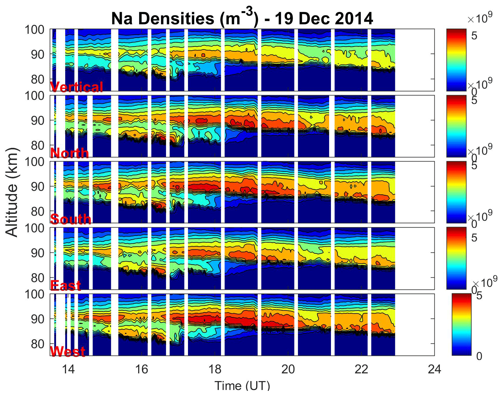
Figure 1 The sodium density measurements from five beam lidar showing formation of a sodium density peak below 85 km (intense from 15:00 to 17:00 UT). The white regions indicate data gaps.

The OH airglow images are 2×2 binned resulting in an image size of 256×256 pixels. While binning increases the signal to noise ratio in the images, the spatial resolution is compromised in the lower elevations. Therefore, we consider the region within 130^∘ field of view for our analysis. The raw airglow images will be curved in the off-zenith regions because they are captured with a fisheye lens in the front end. There are well-established unwarping procedures (Garcia et al., 1997; Narayanan et al., 2009b). We have unwarped the airglow images and projected them in equidistance grids so that the wave parameters can be properly estimated. For unwarping, we assumed that the centroid altitude of OH emission is at 86 km. Before unwarping, we created percentage difference images (I_P) by subtracting and normalizing each individual image (I) with a 1 h running average of the images centered on the individual image ($\stackrel{\mathrm{‾}}{I}$) as given below.

$$\begin{array}{}\text{(3)}& I_{\mathrm{P}}={\displaystyle \frac{I-\stackrel{\mathrm{‾}}{I}}{\stackrel{\mathrm{‾}}{I}}}\times \mathrm{100}\end{array}$$

The wave events are visually identified and cross sections are extracted across the wave events. A strip of 25 pixel width is extracted across the wave signatures in the direction of their propagation. The strip is extracted from a region where the waves are clearly seen and the average of the 25 pixels in each row of the strip results in the intensity cross section, which is detrended afterwards. For a particular wave event, the same region is used for extracting the cross section from different images so that they can be used to estimate the phase velocities of the events. The distances along the cross section are obtained from the spatial coordinates of the pixels corresponding to the center of the strip. The distance value of the last point behind the location of wave events is subtracted so that the distances monotonically increase along the propagation direction of the wave. The wavelength and the phase velocity are obtained from the cross sections extracted from multiple images. The mean values of multiple estimations for the wavelengths and the phase velocities are provided with standard deviations as the errors. The propagation direction is measured within an accuracy of 2^∘. The north is assumed as 0 and the east as 90^∘ azimuths.

On the night of 19 December 2014, the airglow imaging observations started at 14:40 UT and continued until 06:40 UT on 20 December 2014. However, useful mesospheric measurements were available only until 17:20 UT on 19 December 2014 as intense aurora occurred afterwards. The observations after 23:00 UT were hindered by the presence of clouds similar to the lidar measurements.

Our observations being ground based in the Eulerian framework, we cannot observe the same air mass for an extended period. Though we can observe the small-scale structures and their movements in the airglow images, they are also superposed with the background wind, which is derived from the lidar measurements in this work. While this is an unavoidable drawback in studying the atmosphere using ground-based measurements, we assume that the processes occurring are sufficiently homogeneous in the horizontal direction.

Figure 2 The 30 min averages of sodium densities from the vertical beam.

3 Results

3.1 Additional bottom-side peak of the sodium layer

Figure 1 shows the sodium density measurements from the lidar. Note the occurrence of an intense lower-altitude sodium density peak between 15:00 and 17:00 UT, which almost disappeared by about 18:00 UT. This pattern is similar in all five beams, and hence it is clear that the lower-altitude sodium peak formed in an area larger than 35 km × 35 km (or 1225 km²), the minimum distance between the oppositely directed beams. To better investigate the time evolution of the lower-altitude sodium peak, we show the 30 min averages of sodium density profiles from the vertical beam in Fig. 2. By the time of start of the lidar measurements at13:35 UT, a secondary peak that was located closer to the main peak of the sodium layer can already be noticed. Table 1 lists the altitudes and densities of the main peak and the lower-altitude peak. The lower-altitude sodium peak was initially at 87 km, separated by 4 km below the main sodium-layer peak height. With time, both the separation and intensity of the lower-altitude sodium peak increased noticeably. After 15:30 UT, the density of the lower-altitude sodium peak was nearly as intense as the main peak at 91 km, and its peak altitude descended to 82 km, with a separation of 9 km from the main peak of the sodium layer. After 17:00 UT, the lower-altitude sodium peak started to weaken and rapidly disappeared by about 18:00 UT. Figure 2 clearly indicates that the lower-altitude sodium peak was intense and well separated between 15:00 and 17:00 UT, resembling an additional layer, as already seen from the range–time–density maps of Fig. 1.

Table 1 The altitudes and densities of the main and the lower-altitude sodium peaks

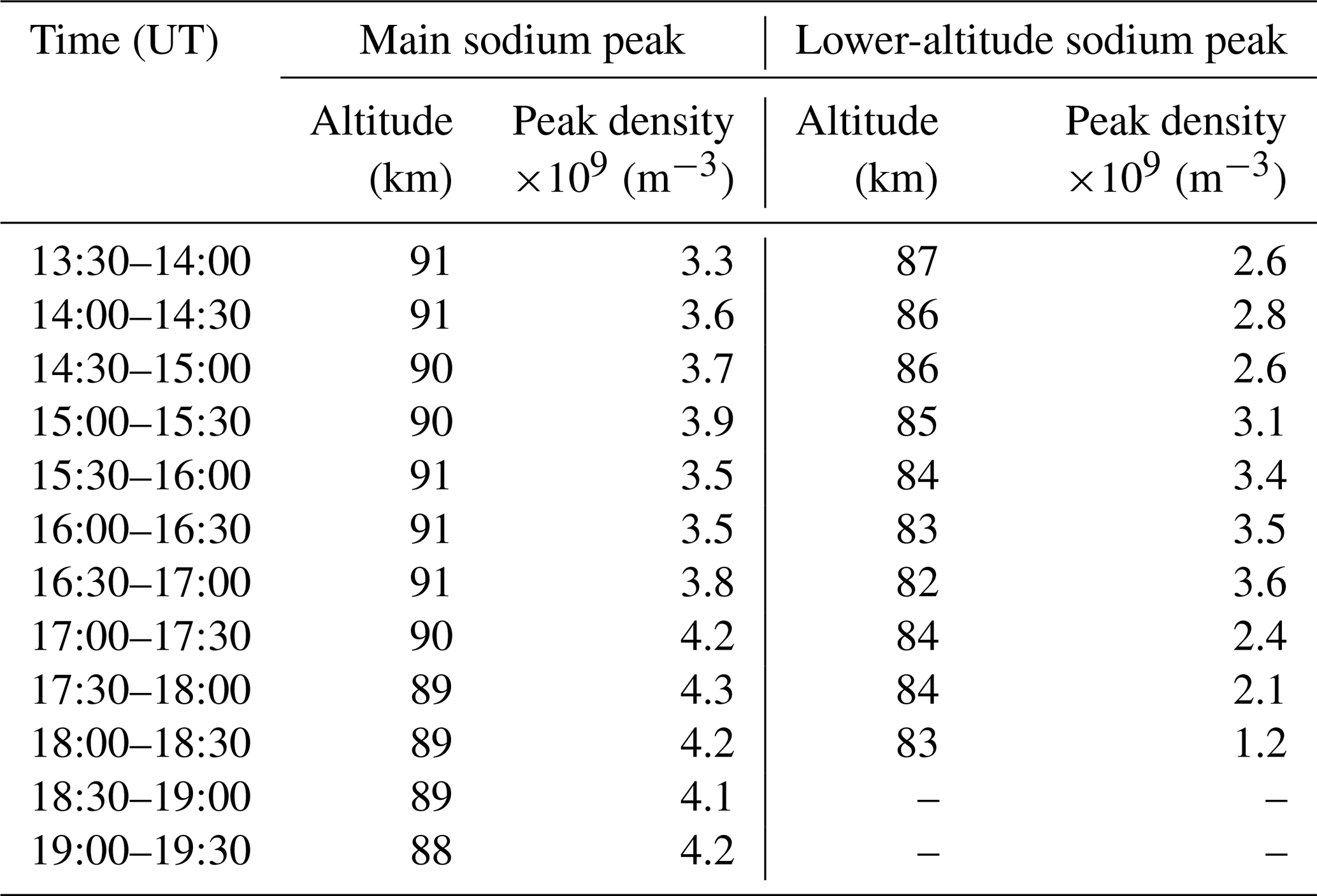
Figure 3 Sodium densities measured by the vertical beam. (a) Column abundance of sodium atoms, (b) range–time–density plot showing coincidence of the column abundance variations with the lower-altitude sodium peak. The dotted black lines in the bottom panel indicate the estimated times of zenith passage of the fronts.

The variation of column abundance of sodium atoms is shown in Fig. 3a along with the range–time–density plot from the vertical beam of the lidar in Fig. 3b. There was a gradual increase in the column abundance during the formation and intensification of the lower-altitude sodium peak. This indicates that the lower-altitude sodium peak is formed due to the production of sodium atoms from some reservoirs instead of from mere redistribution within the existing sodium layer. This is further confirmed by the observation that the column abundance was reduced after the disappearance of the lower-altitude sodium peak. An increase in column-integrated density of 1.85×10¹³ atoms m⁻² occurred during the formation of the lower-altitude sodium peak. There was approximately a 50 % increase in the total column abundance by 16:40 UT compared to the earlier hours around 14:00 UT.

3.2 Passage of mesospheric frontal systems

The airglow imaging of OH emission shows the passage of multiple mesospheric frontal systems as discussed below. The airglow imaging started at 14:40 UT, approximately 1 h after the start of the lidar observations. The passage of an intense mesospheric front can be seen right from the first image acquired. A set of selected images on this night is shown in Fig. 4. In the figure the fronts and the wave observed on the night are marked with arrows indicating their direction of propagation. A corresponding movie is added as supplementary material showing the propagation of successive mesospheric fronts approximately towards the top of the image frame corresponding to the north.

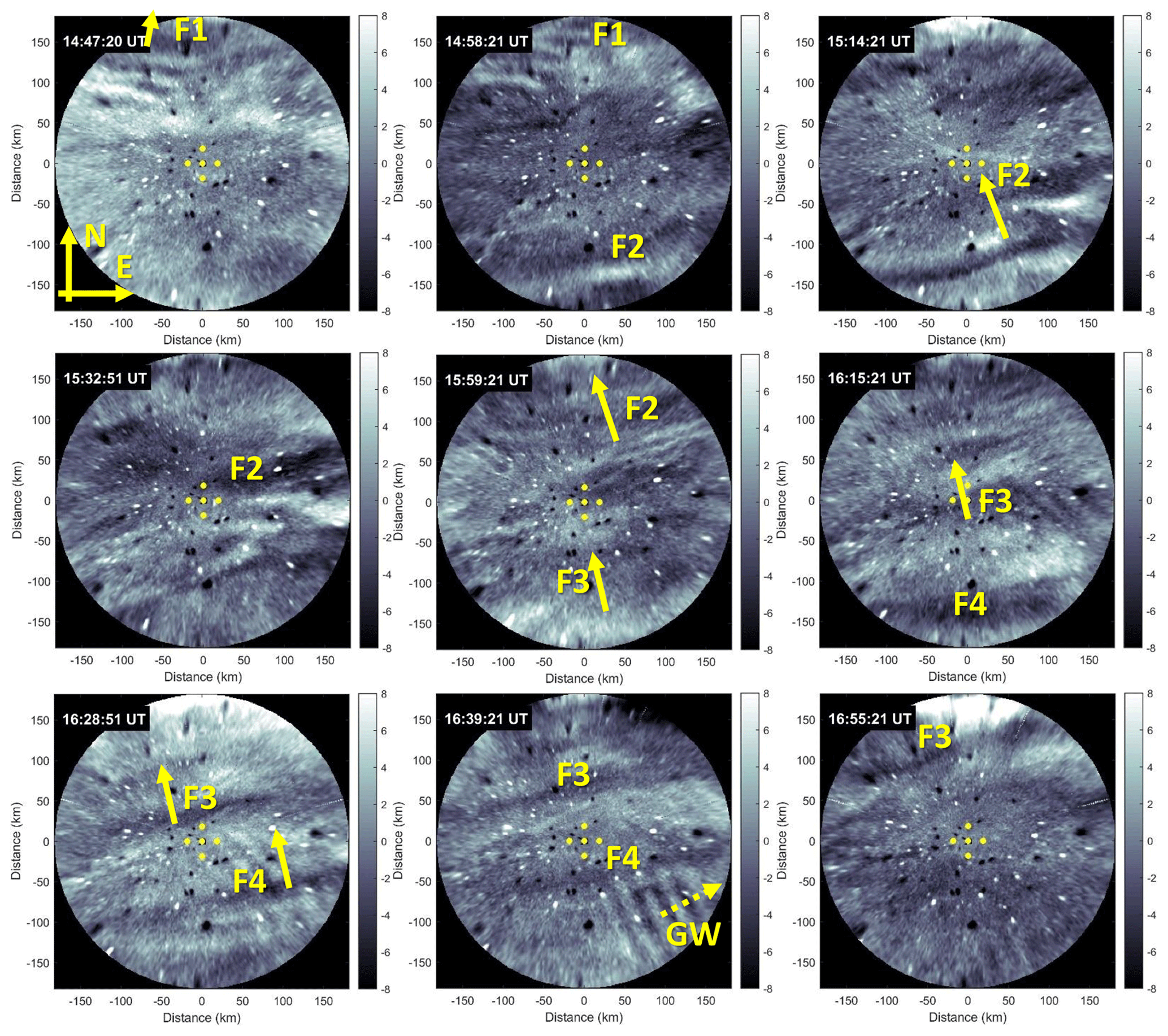
Figure 4 Selected OH airglow images from 19 December 2014. Intensities represent the percentage perturbations according to Eq. (3). The yellow dots near the zenith indicate the location of the lidar beams. The fronts are marked as F and their propagation direction is indicated by an arrow. The gravity wave is indicated as GW with a dashed arrow.

As seen from Fig. 4, the first front (F1) resembled an undular bright mesospheric bore with phase-locked undulations behind the leading front. F1 was moving towards the north at an azimuth of ∼ 3^∘. It has already crossed the zenith region of the observation site, wherein the locations of lidar beams fall as indicated by yellow dots in the images. The estimated wavelength and propagation velocity of the feature are ∼ 23 km and ∼ 63 m s⁻¹ respectively. Since the observations started at a later time, the probable time of zenith passage of F1 is estimated as 14:15 UT based on the calculated phase velocity. Figure 5a shows the cross sections extracted across F1 along its propagation direction. The F1 with trailing undulations can be seen clearly. Further, this front showed the formation of additional wave fronts, which is known to be a characteristic of the mesospheric bores (Dewan and Picard, 1998; Smith et al., 2003). As seen from Fig. 5a, the leading wavefront has reached the edge of the image around 15:00 UT.

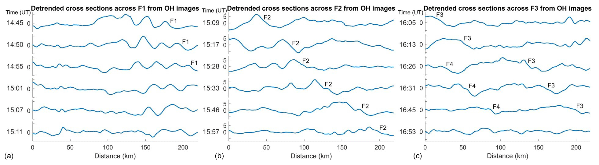
Figure 5 Cross sections extracted and detrended across the fronts from the percentage-differenced OH images. (a) Cross sections across F1, (b) across F2, and (c) across F3 and F4.

The second front (F2) entered the imager field of view from the southern edge around 14:55 UT, and it was also propagating predominantly towards the north with wave normal directed at ∼ 345^∘. There was an enhancement in the OH brightness behind F2. While F2 possessed trailing wave crests, the crests were not as defined as in F1. From the images at 15:14 and 15:32 UT in Fig. 4, it appears that F2 shows some wave-breaking signatures before 15:40 UT. Nevertheless, the cross sections enabled wavelength determination with a value of ∼ 31 km in the earlier part of its observation. F2 showed the formation of waves with a smaller wavelength of ∼ 14 km after 15:45 UT. The front continued to propagate in the same direction with an estimated phase velocity of ∼ 47 m s⁻¹. F2 has crossed the zenith region around 15:38 UT. Figure 5b shows the cross sections across F2. The cross sections also reveal that the trailing undulations initially have larger wavelengths and after 15:40 UT have smaller wavelengths (see the last two rows in Fig. 5b).

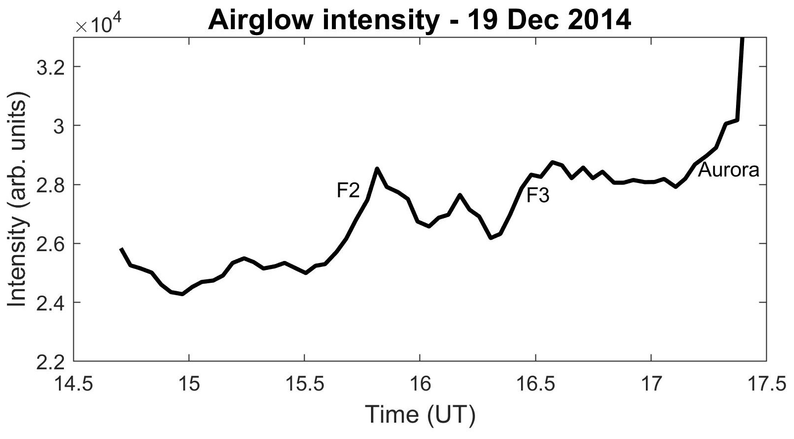
Figure 6 Zenith intensity time series from the average of 16×16 pixels over the zenith of the raw OH images.

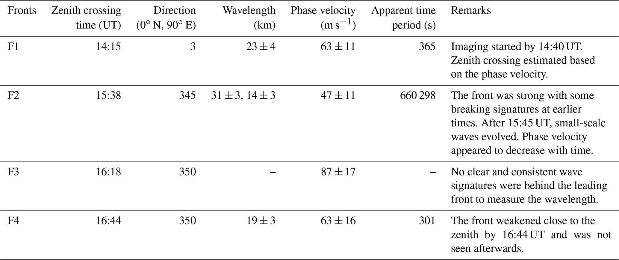
The third front (F3) entered the images from the south around 15:56 UT and propagated across the zenith region by 16:23 UT. No clearly discernable phase-locked undulations were found behind the front. The estimated phase velocity of this front is ∼ 87 m s⁻¹ towards the north at an azimuth of ∼ 350^∘. F3 was the fastest of the observed fronts on this night. The fourth and final front (F4) observed on this night appears to follow F3 along ∼ 350^∘ azimuth. However, it showed few weak phase-locked undulations behind and was moving relatively slow. The estimated wavelength and phase velocity are ∼ 19 km and ∼ 63 m s⁻¹, respectively. Because of the differing phase velocities, the distance between F3 and F4 increased, as can be verified visually from images at 16:15 and 16:39 UT in Fig. 4 and from cross sections in Fig. 5c. F4 became weak and almost unidentifiable in images after 16:45 UT, close to its passage over the zenith. Table 2 lists the characteristics of the fronts. The apparent time periods of the fronts given in the table are obtained as the ratio between the wavelengths and the phase velocities.

Table 2 The physical parameters of the observed fronts

In addition to these four fronts, an east-northeastward propagating gravity wave is also noticed between 16:10 and 16:50 UT. In Fig. 4, it is marked by GW with a dashed arrow indicating its propagation at 16:39 UT. Aurora started to intensify from the northern horizon in the OH images from around 16:55 UT. However, most parts of the images were clear to reveal wave signatures till about 17:20 UT. The auroral features extended southward and completely masked any wave signatures that could have occurred afterwards. This can clearly be seen from Fig. 6, which shows the zenith intensity time series. The intensities are averages of 16×16 pixels surrounding the zenith region of the raw OH images. From Fig. 6, it can be further verified that both F2 and F3 are accompanied by brightness enhancements in OH images indicating that they are bright bores. The sharp increase in intensity associated with aurora are seen from about 17:20 UT. It may be noted that there is no evidence in the past that the aurora enhances OH Meinel band brightness directly. The observed enhancement is due to the entry of auroral light intensities through the broadband filter used to measure the OH Meinel band emissions. Nevertheless, it is worth noting that the signatures of the fronts and the gravity wave weakened significantly by 16:50 UT, well before the aurora masked OH observations. This may also be seen from the last image in Fig. 4.

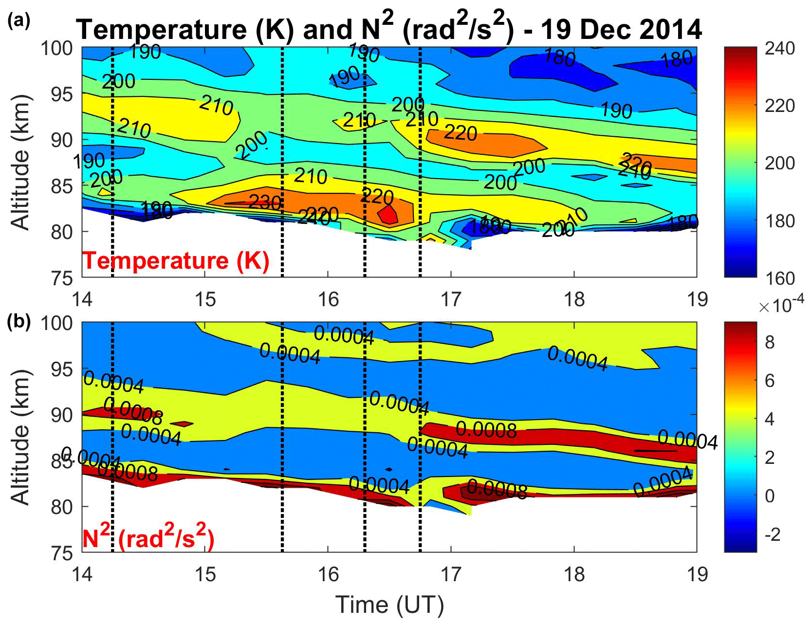
Figure 7 (a) Background temperature structure and (b) square of buoyancy frequency (N²). The dotted black lines indicate the estimated times of zenith passage of the fronts.

3.3 Background temperature and wind conditions

Now we present the background temperature and wind conditions during the above-mentioned observations. Figure 7a shows the background temperatures. The temperature contour shows a downward phase progression at a rate of ∼ 1 km h⁻¹, which might be due to the tidal effects. Of greater interest are the existence of an inversion layer close to 90 km and enhanced temperatures in the lower altitudes coinciding with that of the lower-altitude sodium peak. The temperature enhancement was particularly intense below 85 km in the duration between 15:00 and 17:00 UT. The square of buoyancy frequency profiles (N²) estimated from the temperature contour are shown in Figure 7b. This profile clearly illustrates the existence of an enhanced N² region (shown by yellow and brown) bounded by lower values above and below. This region matches with the altitudes of the thermal inversion. The enhanced N² region also shows a downward progression in concurrence with the downward progression in the temperature contour. Importantly, Fig. 7 shows the existence of a stable thermal ducting region on the night of 19 December 2014. Such regions can support the formation of mesospheric bores as mentioned in Sect. 1. It can be seen that the width of the ducting region decreased after 17:00 UT. The location of the ducting region covers the peak region of main sodium layer prior to 17:00 UT.

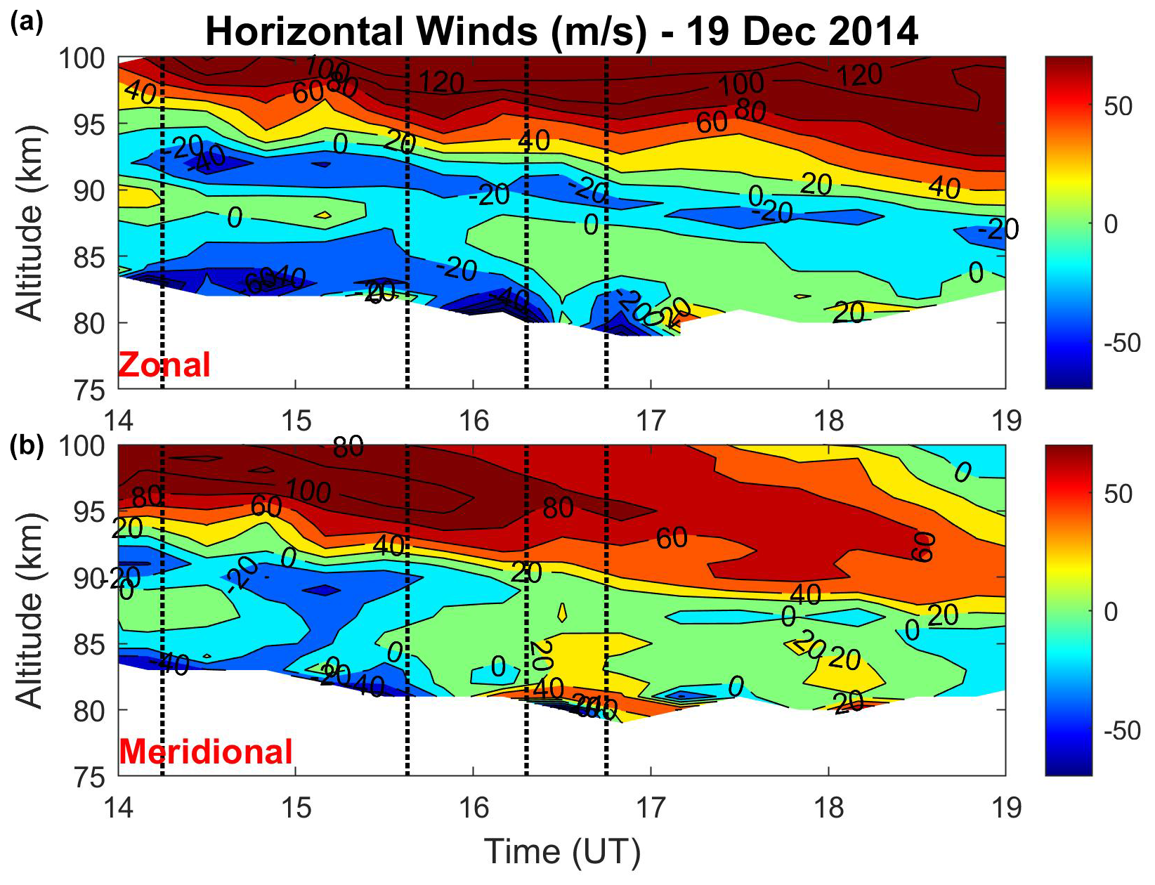
Figure 8 Measured winds: (a) zonal and (b) meridional. The dotted black lines show the estimated times of zenith passage of the fronts.

Figure 9 Vertical shears of the horizontal wind: (a) zonal and (b) meridional. The dotted black lines indicate the estimated times of zenith passage of the fronts.

The zonal and the meridional winds during the observation period are shown in the top and the bottom panels of Fig. 8, respectively. Since all the observed fronts propagated approximately to the north, the meridional winds approximately represent the background wind conditions along the propagation direction of the fronts. In the lower altitudes the wind velocities were within a magnitude of 40 m s⁻¹ in both the zonal and the meridional directions. The meridional winds reversed from southward to northward around 16:00 UT in the altitudes between 83 and 93 km. There was a significant rise in the wind velocities with height, particularly above 93 km before 17:00 UT. The wind magnitudes increased by at least 3 times within a narrow altitude region of about 4 km, indicating the existence of large wind shears. The wind shears are shown in Fig. 9. The shears in the meridional wind were much stronger than those in the zonal wind. Both Figs. 8 and 9 show a downward phase progression very much similar to that seen in the temperature profiles. These large-scale downward-phase-propagating features might be the result of tides.

4 Discussion

The results described above lead to the following important observations that have to be explained: (1) there was a rare formation of intense sodium density peak in the altitudes below 85 km, (2) there was an enhancement in the column abundance of sodium atoms during the formation of this lower-altitude sodium peak and the column abundance started to decline after its disappearance, (3) there were four consecutive mesospheric fronts observed with OH images but not with OI 557.7 nm images coinciding with the duration of this lower-altitude sodium peak, (4) the mesospheric fronts were associated with enhanced OH airglow intensities behind their passages and resembled bright mesospheric bores, (5) temperatures were relatively high in the region of the lower-altitude sodium peak, (6) there was a higher-stability region indicating a thermal ducting structure matching with the altitudes of the main peak of the sodium layer located above the altitudes of lower-altitude sodium peak, and (7) the horizontal winds had intense shears above 93 km along with a reversal in the meridional winds around 16:00 UT in the lower altitudes.

We have seen in Figs. 4, 5 and 6 that the observed fronts were followed by regions of increased OH airglow intensity, indicating that they might be mesospheric bores. F1 showed formation of new undulations as well. However, no clear signatures of the fronts were seen in the OI 557.7 nm emission images. This is surprising given their intense signatures in the OH emission region. The reason appears to be the existence of large wind shear in the region between OH and OI 557.7 nm emission layers, as indicated by Figs. 8 and 9. The fronts appeared to have disappeared owing to the critical level interaction between 93 and 95 km, wherein the background wind speeds surpassed the speed of the observed fronts. This can be seen better with the help of Fig. 10.

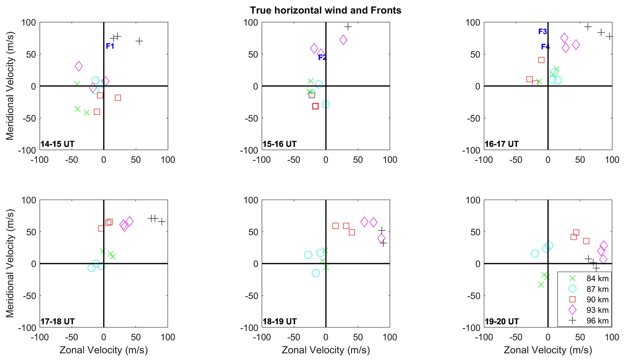
Figure 10 Horizontal wind measurements between 84 and 96 km in 3 km intervals and the phase velocity of the observed fronts in the respective hours.

Figure 10 shows the horizontal winds measured by the lidar in 3 km intervals at the altitudes between 84 and 96 km in every hour. Since we use 20 min averaged data, each height shows three points within every hour. This plot enables us to identify the magnitude and direction of each of the 20 min wind estimates within every hour in the respective altitudes. Also included are the observed velocities of the fronts in the corresponding hours when they were observed. The figure clearly illustrates that the background wind speeds were smaller than the speed of F1 below 93 km but were faster at 96 km. Therefore, the critical level would have occurred in the region between 93 and 96 km restricting F1 from perturbing the higher altitudes. Similarly to the case of F2, F3 and F4, the background wind speeds surpassed the fronts at ∼ 93 km altitudes, resulting in them being filtered and prevented from reaching the higher heights. Particularly interesting is the case of F2. As mentioned earlier, F2 showed breaking signatures and after 15:45 UT revealed the evolution of smaller wavelengths (see Fig. 4 and corresponding discussion in Sect. 3). The small-scale features evolved on the crests of the front shortly after its zenith passage. It is likely that these features are the result of dynamical instabilities due to intense shears revealed in Fig. 9. The billow structures resulting from dynamical instabilities could have perturbed the upper portion of OH airglow layer. The existence of strong winds in the propagation direction of the fronts show the probable reason for not finding them in the OI 557.7 nm images.

The temperature profiles indicate that thermal ducting was possible (Fig. 7) and the wind profiles indicate presence of critical levels immediately above them (Fig. 8). To check the possibility of ducting for the observed fronts, we calculate the vertical wavenumber profiles during their passage over the zenith with the following gravity wave dispersion relation (e.g., Narayanan and Gurubaran, 2013):

$$\begin{array}{}\text{(4)}& m^{\mathrm{2}}={\displaystyle \frac{N^{\mathrm{2}}}{(u-c{)}^{\mathrm{2}}}}-{\displaystyle \frac{u_{zz}}{(u-c)}}+{\displaystyle \frac{u_z}{H(u-c)}}-{\displaystyle \frac{\mathrm{1}}{\mathrm{4}{H}^{\mathrm{2}}}}-k^{\mathrm{2}}.\end{array}$$

In the above equation, m and k stand for the vertical and horizontal wave numbers, respectively; N is the buoyancy frequency; u and c denote the background wind along the wave propagation direction and the phase velocity of the wave, respectively; u_zz and u_z indicate $d^{\mathrm{2}}u/\mathrm{d}{z}^{\mathrm{2}}$ and $\mathrm{d}u/\mathrm{d}z$, respectively; and H is the scale height. Figure 11 shows the calculated m² profiles for each of the fronts with background conditions corresponding to the time of their passage over the zenith. Lines at m² values indicating the vertical wavelengths of 3, 5 km and ∞ are also shown. Since we do not know the horizontal wavenumber k for F3, the last term in Eq. (4) is left out when calculating its vertical wavenumber m.

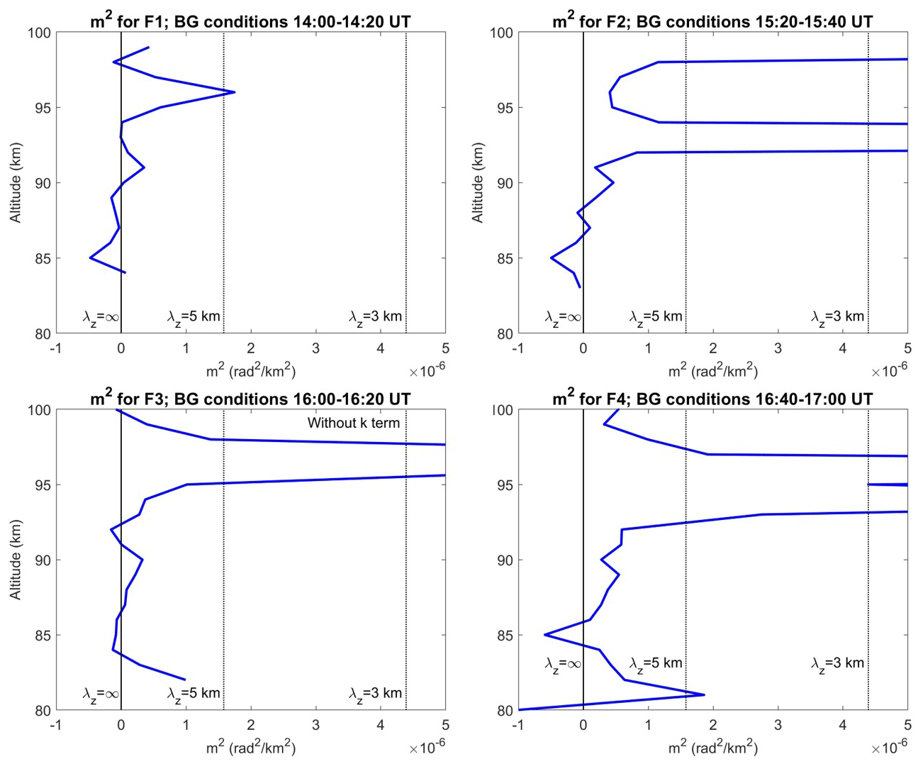
Figure 11 The m² profile for the four fronts. Since F3 did not have trailing undulations, its m² is calculated leaving the k term in Eq. (4). The solid vertical line shows the 0 value, and the dotted vertical lines show m² values corresponding to 5 and 3 km vertical wavelengths.

Generally, a wave undergoes reflection when the m² turns negative in a region. When there is a region of positive m² bounded by the regions of negative m² above and below, the wave becomes ducted. A critical level occurs when the vertical wavelength of a wave approaches 0, and this will be seen as a sharp increase in the m² profile. The critical levels ensure that the wave energy does not propagate beyond the level, but they also contribute to stronger ducting at times. Strong wave reflection may happen when the critical level exists just above a region of stronger stability. In essence, the existence of a critical level at the top of a duct results in a stronger duct because the leakage of energy through the duct is strongly restricted by the critical level wave reflection (Lindzen and Barker, 1985; Skyllingstad, 1991; Ramamurthy et al., 1993). This has happened in the present case, as can be inferred from Fig. 11. In the altitudes below 86 km (90 km for F1) m² values become negative, indicating the lower boundary of the ducting region. In the upper region, there is a very steep increase in the m² values, indicating that strong winds cause the critical levels. By comparing this Fig. 11 with Figs. 7 and 8, one can see that the lower boundary is mainly due to the temperature profile and that the upper boundary is caused by a combination of the wind and temperature profiles (a similar case was observed for a lower atmospheric bore by Ramamurthy et al., 1993). Hence, the important conditions required for formation of the bores were present on the night and the characteristics like enhanced airglow behind the fronts imply that these fronts were bores associated with a sudden downward push causing brightness enhancements in the underlying OH airglow.

The increase of the column abundance of sodium during the formation of the lower-altitude sodium peak is clearly seen from Figs. 1 and 3. To investigate this further, we show the total sodium column abundance along with the column integrated densities from 81 to 88 km, 88 to 95 km, and 95 to 102 km in Fig. 12. Note that the selected altitude ranges correspond to the lower-altitude sodium peak, main layer peak, and the topmost region of atomic sodium layer, respectively. All the densities shown are from the vertical beam. As can be seen from Fig. 12, the shape of the variations in the total column abundance clearly matches with those of the integrated densities of the lower-altitude sodium peak. The lower-altitude sodium peak contributed to about 65 % of the enhancement in the total column abundance. The remaining enhancement was due to the increase in sodium concentration in the higher altitudes. This is also revealed by the red and green lines in Fig. 12. Interestingly, there was a reduction in the sodium densities around 15:30 UT in the altitude range of 88 to 95 km corresponding to the main layer peak. This time matches closely with the passage of F2 over the lidar beams.

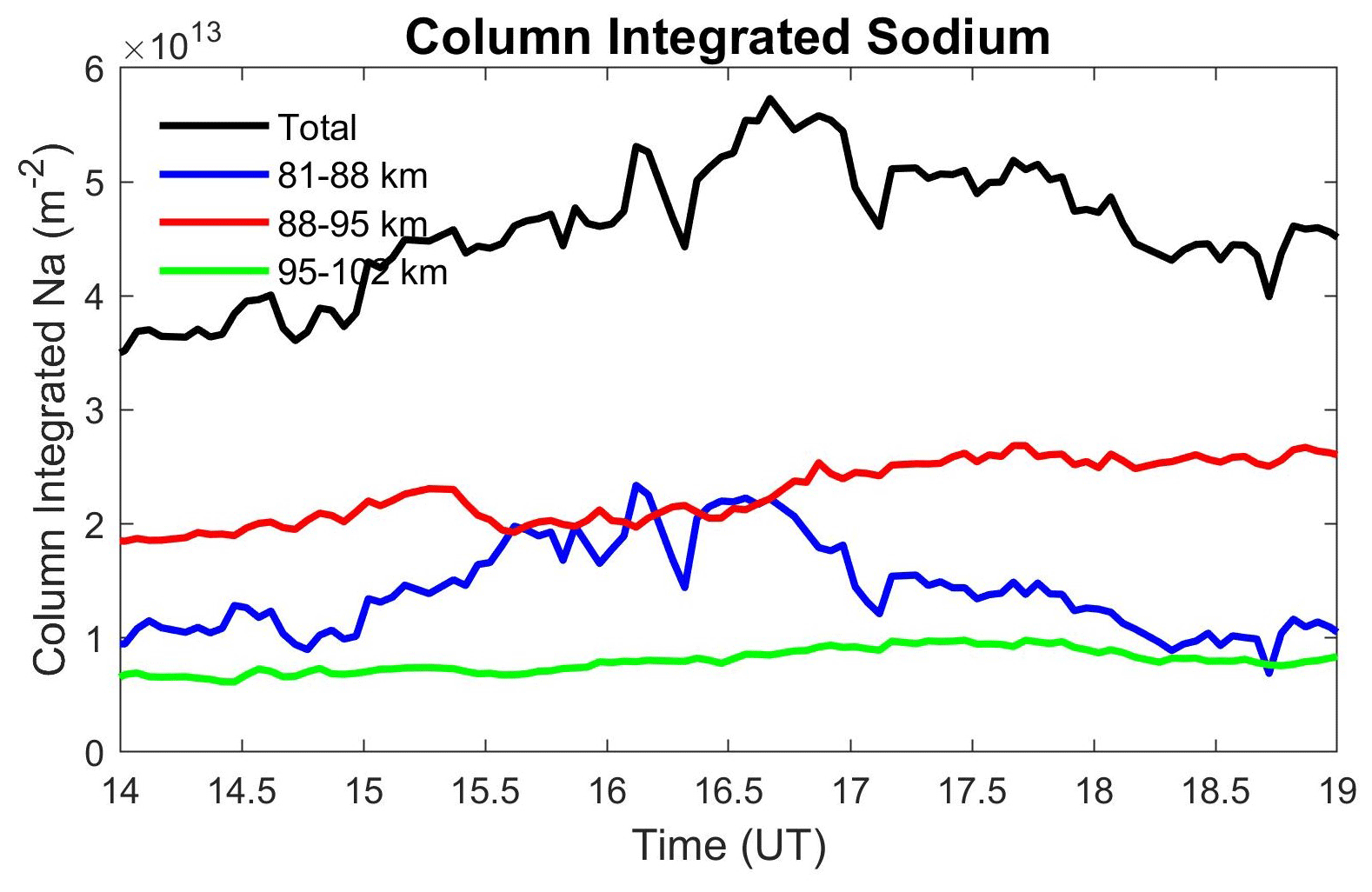
Figure 12 Column-integrated sodium densities in selected altitude regions (blue, red and green lines) to compare with the total column abundance (black line)

The positive correspondence between the sodium density and the temperature variations is already well known (Zhou et al., 1993; Zhou and Mathews, 1995). While there was relatively high temperature in the region of the lower-altitude sodium peak below 85 km, it does not occur on this day alone. Temperatures in the range of 220 to 250 K are fairly common below 85 km in the winter months (Lübken and von Zahn, 1991; Nozawa et al., 2014; Takahashi et al., 2015; Hildebrand et al., 2017). To study the role of temperature in further detail, we show the sodium densities and averaged temperatures separately for the height regions corresponding to the lower-altitude sodium peak (81 to 88 km) and the main sodium peak (88 to 95 km) in Fig. 13. Note that we have used temperature data with 3 min temporal resolution herein so that we can effectively compare them with the sodium density variations. Both densities and temperatures are three-point smoothed in the plots. Figure 13a, c shows the integrated sodium densities and average temperatures for the region of the lower-altitude sodium peak from 81 to 88 km. The temperatures below 83 km are noisy, resulting in large fluctuations. While there are some matching regions between the densities and temperatures, the overall temperature variations differ from that of the sodium density in the lower-altitude peak region. For instance, the sodium densities continued to decrease while temperatures were nearly stable after 17:00 UT. This further indicates that the lower-altitude sodium peak was not merely due to the temperature enhancement. However, the existence of higher temperatures in the lower altitudes is indisputable (see Fig. 7a).

Figure 13b, d show similar plots to those above between the altitude region of 88 and 95 km corresponding to the main sodium layer peak. Note that there was a temperature reduction just before 15:30 UT in this altitude region, which is coincident with the density reduction. F2 has crossed the zenith region around 15:35 UT. It is highly likely that this temperature reduction corresponded to the signature of the passage of F2. The density reduction in the main sodium peak altitudes might therefore be due to the sudden reduction in temperature associated with passage of F2 and downward transport of some of the sodium atoms associated with the bore. It is known that there may be phase delays between the temperature and airglow intensity variations during the passage of mesospheric bores (Taylor et al., 1995; Pautet et al., 2018). For example, the very first report of a mesospheric bore by Taylor et al. (1995) had a temperature signature 15 min prior to the passage of the bore. On the other hand, in the presented observations after 17:15 UT and between 88 and 95 km, the sodium density variations do not, however, correlate with temperature. This may be either due to the horizontal advection of sodium atoms or due to the ion chemistry, as this time also coincides with onset of aurora.

Figure 13 Panels (a) and (b) are integrated sodium densities from 81 to 88 km and 88 to 95 km, respectively. Panels (c) and (d) are averaged temperatures from 81 to 88 km and 88 to 95 km, respectively.

There was supposedly a downward force associated with the bright bores seen as fronts, which brings the minor constituents from the higher altitudes to the lower altitudes. The downward transport will increase the concentrations of minor species whose mixing ratios increase with altitude. This will affect the chemistry of the region. Indeed, such a downward force and associated movement is proposed as a reason for sudden intensity variations following the bore jumps (Dewan and Picard, 1998). It is believed that these bores become bright in OH emission because the OH emission peak moves to lower heights where temperatures are higher (Dewan and Picard, 1998; Medeiros et al., 2005). In this case, the bores are supposed to have occurred in the region between 86 and 93 km (F1 appeared to have occurred a few km higher). The start of the enhanced stability region associated with the temperature inversion around 86 km seems to determine the lower boundary of the duct channel (see Fig. 7). The upper boundary appears to be a combination of the temperature duct along with intense wind shears causing a critical level to the propagating wave-like structures. The bores would have occurred near the center of the duct at ∼ 90 km from where the downward movement would have been initiated. It may be noted that the enhanced temperatures shown in Fig. 7a at altitudes below 85 km also match well with the duration of observation of the fronts. There may be a contribution from adiabatic compression immediately below the altitudes of the duct due to the downward push caused by the bores. However, a detailed investigation on this aspect is beyond the scope of the present work. In addition, such a downward movement also transports minor species, in particular O and H, from the upper altitudes, thereby increasing their concentrations in the lower altitudes. This is because the mixing ratios of O and H increase with altitude in this region, as mentioned above. Not only O and H but also species like Na, O₃ and NaHCO₃ experience downward transport. For example, part of Na below 90 km would have been transported downwards and contributed to the density decrease along with the reduced temperatures seen in the main peak altitudes around 15:30 UT in association with the passage of F2 (see Fig. 13b, d).

It is known that higher H concentration occurring in the region with relatively high temperatures results in higher OH emission rates as per the following reaction.

$$\begin{array}{}\text{(R1)}& \begin{array}{rlr}& \mathrm{H}+{\mathrm{O}}_{\mathrm{3}}\to \mathrm{OH}(\mathit{\nu }\le \mathrm{9})+{\mathrm{O}}_{\mathrm{2}}& \\ & \mathrm{1.4}\times {\mathrm{10}}^{-\mathrm{10}}\exp [-\mathrm{470}/T]\left({\mathrm{cm}}^{\mathrm{3}}{\mathrm{molecule}}^{-\mathrm{1}}{\mathrm{s}}^{-\mathrm{1}}\right)\end{array}\end{array}$$

The Reaction (R1) and its rate constant are taken from Smith and Marsh (2005). It can be seen that Reaction (R1) depends on the temperature and that higher temperatures result in higher reaction rates. Table 3 contains the values of the reaction rates for Eq. (R1) and the other reactions that will be given below. We have given the reaction rates from 200 to 230 K in steps of 10 K. Also indicated are the percentage increases of the reaction rates from 200 to 230 K. As seen from the Table, there will be 36 % increase in the reaction rate of Eq. (R1) when the temperature rises from 200 to 230 K. Therefore, a downward push explains an enhancement in the OH airglow. On 19 December 2014, existence of the strong thermal ducting in the region coincident with the altitudes of main sodium layer peak would have favored formation of a mesospheric bore generating such a downward force and transport of minor species.

Table 3 Values of the reaction rates and their percentage increases for temperatures from 200 to 230 K (units of the reaction rates are given in the respective rate expressions)

Now we discuss how the sodium chemistry is affected by an increased concentration of minor species, particularly H and O, due to the downward transport. Though all the minor species existing below 90 km would have experienced a downward push due to the passages of bores, we discuss the chemistry with focus on O and H because they are the principal minor species connecting different reactions. At altitudes above 90 km, the densities and collisions are so low that formation of complex multi-atomic molecules are often difficult. Further, during the day UV photon flux contributes to the dissociation of complex larger molecules. In the lower altitudes, a larger portion of the sodium atoms react with other atoms and molecules and form reservoir species. The most important reservoir species for sodium is NaHCO₃, which liberates sodium atoms when interacting with H (Plane, 2004; Plane et al., 2015).

$$\begin{array}{}\text{(R2)}& \begin{array}{rl}& {\mathrm{NaHCO}}_{\mathrm{3}}+\mathrm{H}\to \mathrm{Na}+{\mathrm{H}}_{\mathrm{2}}{\mathrm{CO}}_{\mathrm{3}}\\ & \mathrm{1.84}\times {\mathrm{10}}^{-\mathrm{13}}{T}^{\mathrm{0.777}}\exp [-\mathrm{1014}/T]\\ & \left({\mathrm{cm}}^{\mathrm{3}}{\mathrm{molecule}}^{-\mathrm{1}}{\mathrm{s}}^{-\mathrm{1}}\right)\end{array}\end{array}$$

In addition, NaOH and NaO can also liberate sodium as given below while interacting with H and O, respectively.

$$\begin{array}{}\text{(R3)}& {\displaystyle }\begin{array}{rl}& \mathrm{NaOH}+\mathrm{H}\to \mathrm{Na}+{\mathrm{H}}_{\mathrm{2}}\mathrm{O}\mathrm{4}\times {\mathrm{10}}^{-\mathrm{11}}\exp [-\mathrm{550}/T]\\ & \left({\mathrm{cm}}^{\mathrm{3}}{\mathrm{molecule}}^{-\mathrm{1}}{\mathrm{s}}^{-\mathrm{1}}\right)\end{array}\text{(R4)}& {\displaystyle }\begin{array}{rl}& \mathrm{NaO}+\mathrm{O}\to \mathrm{Na}+{\mathrm{O}}_{\mathrm{2}}\mathrm{2.2}\times {\mathrm{10}}^{-\mathrm{10}}\sqrt{T/\mathrm{200}}\\ & \left({\mathrm{cm}}^{\mathrm{3}}{\mathrm{molecule}}^{-\mathrm{1}}{\mathrm{s}}^{-\mathrm{1}}\right)\end{array}\end{array}$$

Reactions (R2)–(R4) and corresponding rate constants are taken from Plane (2004), Gómez Martín et al. (2016). While Reactions (R2)–(R4) are all dependent on temperature, the temperature dependence is weak for Reaction (R4). Reaction (R2) has a significant activation energy and hence is strongly dependent on temperature, as can be seen from its rate expression. For example, a 30 K increase in temperature from 200 K will increase the reaction rate by 116 %, as given in Table 3.

Reactions (R2) and (R3) clearly show that more sodium can be liberated when atomic H is transported from the higher altitudes. There is sufficient atomic H in the region between 80 and 90 km (e.g., Plane et al., 2015, Fig. 4) that the downward flux increases the concentration and mixing ratio of H in heights below 85 km. The mixing ratio of NaHCO₃ decreases with altitude in the region between 85 and 90 km and increases at lower altitudes with peak concentration occurring around 84 km. The lower-altitude sodium peak forms in the region where the concentration of NaHCO₃ is supposed to peak (Plane, 2004, Fig. 5). Therefore, there will be sufficient concentrations of reservoir species in the region, and the rate with which the sodium-liberating reactions occur will be higher when the temperature is higher. Since the temperatures were comparatively high below 85 km, more sodium atoms would have liberated resulting in a pronounced lower-altitude sodium peak, which appears as a secondary sodium layer in the lower altitudes. Due to relatively low values of temperature in the altitudes between 84 and 88 km, the amount of liberated sodium will be smaller in spite of the downward transport of minor species. In addition, in those heights the downward transport occurs in the region of decreasing mixing ratio of NaHCO₃, the most important reservoir species of sodium. This explains an apparent gap between the main peak and the lower-altitude peak of the sodium layer.

The principal loss of sodium atoms below 85 km is through the formation of NaHCO₃, NaOH, NaO,NaO₂ and meteoric smoke particles. However, atomic sodium undergoes only the following two reactions directly, whose products further react with minor species in the mesosphere to produce more stable reservoirs like NaHCO₃.

$$\begin{array}{}\text{(R5)}& {\displaystyle }\begin{array}{rl}& \mathrm{Na}+{\mathrm{O}}_{\mathrm{3}}\to \mathrm{NaO}+{\mathrm{O}}_{\mathrm{2}}\mathrm{1.1}\times {\mathrm{10}}^{-\mathrm{9}}\exp [-\mathrm{116}/T]\\ & \left({\mathrm{cm}}^{\mathrm{3}}{\mathrm{molecule}}^{-\mathrm{1}}{\mathrm{s}}^{-\mathrm{1}}\right)\end{array}\text{(R6)}& {\displaystyle }\begin{array}{rl}& \mathrm{Na}+{\mathrm{O}}_{\mathrm{2}}+M\to {\mathrm{NaO}}_{\mathrm{2}}+M\\ & \mathrm{5.0}\times {\mathrm{10}}^{-\mathrm{30}}[T/\mathrm{200}{]}^{-\mathrm{1.22}}\\ & \left({\mathrm{cm}}^{\mathrm{6}}{\mathrm{molecule}}^{-\mathrm{2}}{\mathrm{s}}^{-\mathrm{1}}\right)\end{array}\end{array}$$

The reactions and corresponding rates are taken from Plane et al. (2015). The Reaction (R6) decreases with increase in temperature (see Table 3) and is of secondary importance compared to Reaction (R5). Therefore, in the region of lower-altitude sodium peak where the temperatures were higher, the removal of sodium atoms by O₂ was weaker.

Reaction (R5) depends on O₃ concentration. The O₃ concentration peaks between 90 and 95 km in the mesosphere, and hence the mixing ratio increases with altitude in the region of downward transport (Smith and Marsh, 2005). This indicates that some of the O₃ will also be transported downwards. However, the concentration of O₃ depends on the concentrations of H, O and temperature. The production of O₃ is through the three-body reaction given in Reaction (R7), which is inversely dependent on temperature. The generated O₃ is removed by H through Reaction (R1) and O through Reaction (R8). Both these reactions are faster in higher temperatures.

$$\begin{array}{}\text{(R7)}& {\displaystyle }\begin{array}{rl}& \mathrm{O}+{\mathrm{O}}_{\mathrm{2}}+M\to {\mathrm{O}}_{\mathrm{3}}+M\mathrm{6.0}\times {\mathrm{10}}^{-\mathrm{34}}[\mathrm{300}/T{]}^{\mathrm{2.4}}\\ & \left({\mathrm{cm}}^{\mathrm{6}}{\mathrm{molecule}}^{-\mathrm{2}}{\mathrm{s}}^{-\mathrm{1}}\right)\end{array}\text{(R8)}& {\displaystyle }\begin{array}{rl}& \mathrm{O}+{\mathrm{O}}_{\mathrm{3}}\to {\mathrm{O}}_{\mathrm{2}}+{\mathrm{O}}_{\mathrm{2}}\mathrm{8.0}\times {\mathrm{10}}^{-\mathrm{12}}\exp [-\mathrm{2060}/T]\\ & \left({\mathrm{cm}}^{\mathrm{3}}{\mathrm{molecule}}^{-\mathrm{1}}{\mathrm{s}}^{-\mathrm{1}}\right)\end{array}\end{array}$$

The two reactions above and the corresponding rates are from Smith and Marsh (2005). Reaction (R1) is the major sink for O₃ during nighttime, and the rate of Reaction (R8) increases enormously with temperature as given in Table 3, thereby further reducing the O₃ concentration. Therefore, the down-flux of H and O to the relatively higher temperature regions result in larger removal of O₃ despite its down-flux. This reduction of O₃ in turn affects the effectiveness of removal of the liberated sodium atoms through Reaction (R5) in the lower altitudes. The above discussion indicates that sodium densities can increase when H and O are transported downwards along with other minor species when the temperatures in the lower altitudes are relatively high.

As mentioned earlier, we have seen from Reaction (R1) that the OH airglow intensity also increases when there is a downward flux along with higher temperatures, and this also coincides with the destruction of O₃. All these observations indicate that the temperature and wind structure in the 86 to 93 km region lead to an intense ducting region where the observed mesospheric bores could have formed. The associated downward transport of minor species caused by the bores have led to the liberation of fresh sodium atoms in the lower altitudes from corresponding reservoirs according to Reactions (R2)–(R4). Further, the reconversion of sodium to reservoir species would have been restricted due to the reduction in O₃ concentrations and relatively high temperatures. This can explain the link between the observation of multiple mesospheric bores, formation of the lower-altitude sodium peak and the enhancement in the column-integrated sodium densities in the same duration. After the weakening and disappearance of the fronts, the downward transport of minor species would have stopped resulting in the removal of sodium by regeneration of the reservoir species from atomic sodium in the lower altitudes. Further, it may be noted that the temperatures below 85 km also decreased after the disappearance of the fronts.

Because we did not have airglow imaging observations before 14:40 UT and aurora appeared after 17:15 UT, we are unable to probe the origins of the mesospheric fronts identified as bores. Moreover, the focus of the present work is towards understanding the unusual formation of the bottom-side lower-altitude sodium peak and its relation to the observed mesospheric fronts rather than studying the formation of the mesospheric fronts themselves. The lower-altitude sodium peak occurred at altitudes that are too low for the ion chemistry to play any important role and hence we did not discuss the ion chemistry associated with the sodium production.

5 Conclusions

In this work, we discuss the sodium lidar and airglow imaging observations made on 19 December 2014 from Ramfjordmoen (69.6^∘ N, 19.2^∘ E) near Tromsø, Norway. An unusual occurrence of a lower-altitude sodium peak below 85 km was noticed following the passage of four successive mesospheric frontal events observed in the OH airglow images (Figs. 1–3). The fronts resembled bright mesospheric bores showing an enhancement in the OH airglow intensity following their passage (Figs. 4–6). The existence of a favorable ducting region for formation of the bores was present (Fig. 11). Both the temperature and the wind profiles (Figs. 7 and 8) contributed to the duct. The horizontal winds showed an intense shearing region from ∼ 93 km in altitude (Fig. 9). The critical levels occurring in this region restricted the propagation of the fronts to the OI 557.7 nm airglow altitudes (Figs. 10 and 11). The temperatures in the lower altitudes were in the range of 220 to 250 K during the formation of lower-altitude sodium peak (Fig. 7). While this magnitude of temperatures is not uncommon in the altitudes below 85 km, on this night the temperature enhancement coincided with the duration of the fronts. An enhancement in the column abundance of sodium was also seen to occur coincidentally with the formation of the lower-altitude sodium peak (Figs. 3 and 12). Further analysis showed that the temperature alone cannot explain the formation of the lower-altitude sodium peak (Fig. 13). We explain the observations consistently as follows.

The strong ducting appears to have provided favorable conditions for the formation of multiple mesospheric bores that are observed as frontal features in the OH images. The downward transport of air rich in minor species like H and O associated with the mesospheric bores appeared to result in an enhancement of OH airglow intensity and the release of atomic sodium from the reservoir species in the lower altitudes. The existence of a relatively high temperature region below 85 km compared to the temperatures in the higher altitudes could have led to increased reaction rates enabling larger release of sodium atoms from reservoir species like NaHCO₃ and NaOH. The removal of atomic sodium by reformation of reservoir species seemed to have further reduced under the conditions of enhanced temperature with down-flux of H and O. After 16:45 UT, the fronts weakened and disappeared, thereby reducing the downward supply of the H, O and other minor species like NaHCO₃. The temperatures below 85 km were also decreased after the weakening of the fourth front. This could have resulted in reconversion of the atomic sodium to sodium reservoir species, which was seen as reduction in the column abundance of sodium and disappearance of the lower-altitude sodium peak.

This event brings interesting new insights as follows. (1) On rare occasions intense sodium peaks form below the main sodium layer peak. (2) The mesospheric bores play an important role in altering the minor species concentrations in the mesospheric region within short temporal durations. (3) Multiple mesospheric bores can form with different phase velocities within a few hours.