Validation of aerosol backscatter profiles from Raman lidar and ceilometer using balloon-borne measurements

Remote-sensing measurements by light detection and ranging (lidar) instruments are fundamental for the monitoring of altitude-resolved aerosol optical properties. Here we validate vertical profiles of aerosol backscatter coefficient (β_aer) measured by two independent lidar systems using co-located balloon-borne measurements performed by Compact Optical Backscatter Aerosol Detector (COBALD) sondes. COBALD provides high-precision in situ measurements of β_aer at two wavelengths (455 and 940 nm). The two analyzed lidar systems are the research Raman Lidar for Meteorological Observations (RALMO) and the commercial CHM15K ceilometer (Lufft, Germany). We consider in total 17 RALMO and 31 CHM15K profiles, co-located with simultaneous COBALD soundings performed throughout the years 2014–2019 at the MeteoSwiss observatory of Payerne (Switzerland). The RALMO (355 nm) and CHM15K (1064 nm) measurements are converted to 455 and 940 nm, respectively, using the Ångström exponent profiles retrieved from COBALD data. To account for the different receiver field-of-view (FOV) angles between the two lidars (0.01–0.02^∘) and COBALD (6^∘), we derive a custom-made correction using Mie-theory scattering simulations. Our analysis shows that both lidar instruments achieve on average a good agreement with COBALD measurements in the boundary layer and free troposphere, up to 6 km altitude. For medium-high-aerosol-content measurements at altitudes below 3 km, the mean ± standard deviation difference in β_aer calculated from all considered soundings is −2 % ± 37 % (−0.018 ± 0.237 Mm⁻¹ sr⁻¹ at 455 nm) for RALMO−COBALD and +5 % ± 43 % (+0.009 ± 0.185 Mm⁻¹ sr⁻¹ at 940 mm) for CHM15K−COBALD. Above 3 km altitude, absolute deviations generally decrease, while relative deviations increase due to the prevalence of air masses with low aerosol content. Uncertainties related to the FOV correction and spatial- and temporal-variability effects (associated with the balloon's drift with altitude and different integration times) contribute to the large standard deviations observed at low altitudes. The lack of information on the aerosol size distribution and the high atmospheric variability prevent an accurate quantification of these effects. Nevertheless, the excellent agreement observed in individual profiles, including fine and complex structures in the β_aer vertical distribution, shows that under optimal conditions, the discrepancies with the in situ measurements are typically comparable to the estimated statistical uncertainties in the remote-sensing measurements. Therefore, we conclude that β_aer profiles measured by the RALMO and CHM15K lidar systems are in good agreement with in situ measurements by COBALD sondes up to 6 km altitude.

1 Introduction

Aerosol particles are ubiquitous in the atmosphere and play a key role in multiple processes that affect weather and climate. They absorb and scatter the incoming and outgoing radiation, which affects the Earth's radiative budget (direct effect), and interact with cloud formation processes, influencing their microphysical properties and lifetime (indirect effect) (e.g., Haywood and Boucher, 2000). Atmospheric aerosols are one of the largest sources of uncertainty in current estimates of anthropogenic radiative forcing (Bindoff et al., 2013).

Among the most significant causes of this uncertainty is the high variability in space and time in the aerosol's concentration, composition and optical properties. Remote-sensing instruments, such as light detection and ranging (lidar) systems, represent an optimal tool for the monitoring of altitude-resolved aerosol optical coefficients (backscatter and extinction), especially in the planetary boundary layer (PBL) (e.g., Amiridis et al., 2005; Navas-Guzmán et al., 2013). Lidar networks like EARLINET (https://www.earlinet.org, last access: 27 January 2021) and E-PROFILE (https://www.eumetnet.eu/e-profile, last access: 27 January 2021), comprising several hundreds of single-wavelength (including ceilometers) and multi-wavelength (Raman) lidars, provide a comprehensive database of the horizontal, vertical and temporal distribution of aerosols over Europe (e.g., Bösenberg et al., 2003; Pappalardo et al., 2014; Sicard et al., 2015).

Lidar instruments offer the advantages of vertically resolved measurements and continuous operation in time but are subject to a number of intrinsic uncertainties of this technique. Single-wavelength elastic-backscatter lidars are limited by the fact that only one signal is measured, while the returning intensity is determined by two parameters (backscatter and extinction). Hence, an a priori assumption on the aerosol extinction-to-backscatter ratio (the so-called “lidar ratio”) is necessary for the calculation of the aerosol backscatter profiles (e.g., Collis and Russel, 1976). Additionally, the retrieval at low altitudes is particularly challenging because of the incomplete geometric overlap between the incoming beam and the receiver's field of view (e.g., Wandinger and Ansmann, 2002; Weitkamp, 2005; Navas-Guzmán et al., 2011). Previous comparison studies in the context of EARLINET found typical deviations of 10 % in aerosol backscatter coefficient (Matthais et al., 2004) and up to 30 % in attenuated backscatter (Tsaknakis et al., 2011; Madonna et al., 2018) between elastic-backscatter lidars and more advanced Raman lidar measurements in the PBL.

Multi-wavelength Raman lidars allow the independent measurement of aerosol backscatter and extinction as functions of altitude by the detection of a pure molecular-backscatter signal in addition to the elastic backscatter (Ansmann et al., 1990, 1992). However, the retrieval procedure is complex and prone to uncertainties, in particular for extinction. It involves the calculation of the derivative of the logarithm of the ratio between the atmospheric number density of molecules and the lidar-received power, which generally requires complex data-handling techniques to isolate the signal from statistical fluctuations (Pappalardo et al., 2004). The comparison of different aerosol backscatter retrieval algorithms between 11 Raman lidar systems in EARLINET, using synthetic input data, showed deviations between them up to 20 % for altitudes below 2 km (Pappalardo et al., 2004). This calls for careful validation studies against independent in situ measurements, as we perform in this work.

In situ instruments are characterized by higher precision and signal-to-noise ratio compared to remote-sensing measurements but are typically limited by low spatial and temporal coverage. Altitude-resolved in situ measurements of aerosol optical properties can be achieved by various platforms including aircrafts, unmanned aerial vehicles (UAVs) and meteorological balloons. Specifically, balloon-borne measurements of aerosol backscatter are typically used to investigate high-altitude cirrus clouds (e.g., Khaykin et al., 2009; Cirisan et al., 2014) and aerosol layers in the upper troposphere and stratosphere (e.g., Rosen and Kjome, 1991; Vernier et al., 2015; Brunamonti et al., 2018), which are not accessible by aircrafts and UAVs. The aim of this paper is to use balloon-borne measurements of aerosol backscatter in the lower troposphere to validate the retrievals of aerosol backscatter coefficient by one co-located Raman lidar and one co-located ceilometer.

The instruments and data used for the comparison are introduced in detail in Sect. 2. The method of comparison, including the derivation of a field-of-view (FOV) correction from idealized Mie-theory scattering simulations, is described in Sect. 3. The results of the comparison are discussed in Sect. 4 and the conclusions summarized in Sect. 5.

2 Observations

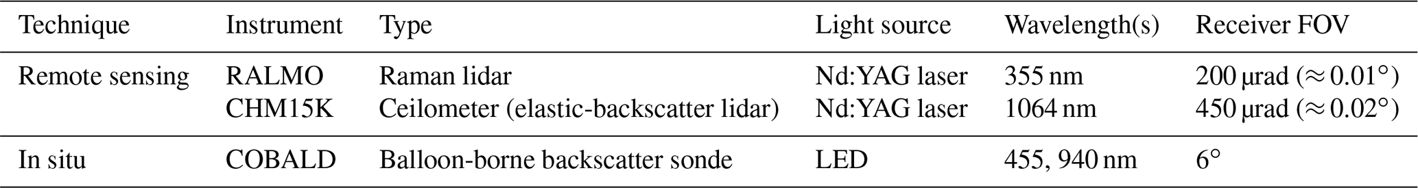
We analyze vertical profiles of aerosol backscatter coefficient (β_aer) measured by two remote-sensing instruments, namely one research Raman lidar system and one commercial ceilometer, and in situ (balloon-borne) measurements performed by aerosol backscatter sondes. The three instruments and measuring techniques are introduced in Sects. 2.1 and 2.2, and their main characteristics are summarized in Table 1. All data were collected at the MeteoSwiss Aerological Observatory of Payerne, Switzerland (46.82^∘ N, 6.95^∘ E), located at an elevation of 491 m above sea level (a.s.l.), between January 2014 and October 2019. The selection of the dataset considered for the statistical comparison is described in Sect. 2.3. Spatial and temporal variability issues, related to the different characteristics of the lidar and balloon-sounding techniques, are discussed in Sect. 2.4.

Table 1 Summary of the main technical characteristics of the three instruments used in this work, including measuring technique, instrument type, light-emitting source, wavelengths and receiver FOV angle.

2.1 Remote-sensing measurements

RALMO (Raman Lidar for Meteorological Observations) is a research Raman lidar system developed by EPFL Lausanne in collaboration with MeteoSwiss (Dinoev et al., 2013), operational in Payerne since 2008 and part of the EARLINET network. It uses a Nd:YAG laser source, which emits pulses of 8 ns duration at a wavelength of 355 nm and frequency of 30 Hz. The laser beam divergence is 120 µrad and the mean energy per pulse 400 mJ. The receiving system consists of four telescopes with 30 cm parabolic mirrors, with equivalent total aperture of 60 cm and field of FOV angle of 200 µrad. Optical fibers connect the telescope mirrors with two polychromators, which allow us to isolate the rotational–vibrational Raman signals of nitrogen and water vapor (wavelengths of 386.7 and 407.5 nm, respectively) and the pure rotational Raman lidar signals (around 355 nm). The rotational–vibrational signals are used to derive water vapor profiles (Brocard et al., 2013; Hicks-Jalali et al., 2019, 2020), while the pure rotational signals are used for temperature, aerosol backscatter and aerosol extinction coefficients (e.g., Dinoev et al., 2010; Martucci et al., 2018). The optical signals are detected by photomultipliers and acquired by a transient recorder system (Brocard et al., 2013). Thanks to its Raman technique, RALMO retrievals are unaffected by incomplete overlap issues. Nevertheless, the signal-to-noise ratio is typically very low in the first 200 m above the station; therefore this altitude region is not considered in this study. Aerosol backscatter coefficient measurements from RALMO were recently used to characterize hygroscopic growth during mineral dust and smoke events (Navas-Guzmán et al., 2019). Here we derive the RALMO β_aer at 355 nm from the ratio between the elastic and inelastic signal, as described in Navas-Guzmán et al. (2019).

The CHM 15K NIMBUS (hereafter CHM15K) ceilometer is a single-wavelength elastic-backscatter lidar manufactured by Lufft, Germany (Lufft, 2019), installed in Payerne since 2012, and a member of E-PROFILE. It uses a Nd:YAG narrow-beam microchip laser emitting 1 ns pulses at a wavelength 1064 nm and repetition rate between 5–7 Hz, with a receiver FOV of 450 µrad. It supports a range up to 15 km with a first overlap point at 80 m and full overlap reached at 800 m above the station (Hervo et al., 2016). Below this level, the profiles are corrected for incomplete overlap (Hervo et al., 2016). CHM15K is employed as a cloud height sensor and for the automatic detection of boundary layer height (Poltera et al., 2017), and it was used for the characterization of aerosol hygroscopic properties (Navas-Guzmán et al., 2019). Here we derive β_aer at 1064 nm from the CHM15K elastic signal using a Klett inversion algorithm (Klett, 1981). This technique was shown to provide accurate aerosol backscatter profiles despite the low molecular backscatter at infrared wavelengths and the low signal-to-noise ratio of a ceilometer in the free troposphere (Wiegner and Geiss, 2012). In particular, using a similar system (CHM15kx by Jenoptik, Germany), Wiegner and Geiss (2012) report a relative error of 10 % in β_aer at 1064 nm retrieved by this method. For consistency within our statistical comparison, here we assume a constant lidar ratio equal to 50 sr for all profiles. The uncertainty related to this assumption is discussed in Sect. 4.3.

2.2 In situ measurements

COBALD (Compact Optical Backscatter Aerosol Detector) is a lightweight (500 g) aerosol backscatter detector for balloon-borne measurements developed at ETH Zürich, based on the original prototype by Rosen and Kjome (1991). Using two light-emitting diodes (LEDs) as light sources and a photodiode detector with FOV of 6^∘, COBALD provides high-precision in situ measurements of aerosol backscatter at wavelengths of 455 nm (blue visible) and 940 nm (infrared). COBALD was originally developed for the observation of high-altitude clouds, such as cirrus (e.g., Brabec et al., 2012; Cirisan et al., 2014) and polar stratospheric clouds (Engel et al., 2014), while recently it was proven able to detect and characterize aerosol layers in the upper troposphere–lower stratosphere (e.g., Vernier et al., 2015, 2018; Brunamonti et al., 2018). In this work, for the first time we use COBALD measurements for the analysis of boundary layer and lower-tropospheric aerosols.

For each balloon sounding, the COBALD sonde is connected to a host radiosonde via their XDATA interface (e.g., Wendell and Jordan, 2016) to transmit the data to the ground station. The average ascent rate of the balloon is set to around 5 m s⁻¹, which combined with a measurement frequency of 1 Hz provides a vertical resolution of approximately 5 m. Typical balloon burst altitude is about 35 km. Due to the high sensitivity of its photodiode detector, COBALD sondes can be only deployed during nighttime. Hence, all soundings analyzed here were started at approximately 23:00 UTC. More than 100 COBALD soundings were performed in Payerne since 2009, supported by SRS-C34 radiosondes by MeteoLabor, Switzerland (MeteoLabor, 2010), until December 2017, and RS41-SGP radiosondes by Vaisala, Finland (Vaisala, 2017), since January 2018.

The COBALD measurements are typically expressed as backscatter ratio (BSR), defined as the ratio of the total-to-molecular-backscatter coefficient (Eq. 1), at 455 and 940 nm. The BSR is obtained by dividing the total measured signal (normalized to the altitude-dependent LED emitted power) by its molecular contribution, which is computed from the atmospheric extinction according to Bucholtz (1995). The atmospheric number density of molecules is derived from the radiosonde measurements of temperature and pressure (e.g., Cirisan et al., 2014). Accuracy and precision of COBALD BSR were estimated by Vernier et al. (2015) as 5 % and 1 %, respectively, at upper-tropospheric conditions. Here, we further derive β_aer from the COBALD BSR assuming a molecular-extinction-to-backscatter ratio of $\mathrm{8}\mathit{\pi }/\mathrm{3}$ sr.

$$\begin{array}{}\text{(1)}& \mathrm{BSR}={\displaystyle \frac{{\mathit{\beta }}_{\mathrm{aer}}+{\mathit{\beta }}_{\mathrm{mol}}}{{\mathit{\beta }}_{\mathrm{mol}}}}\end{array}$$

2.3 Dataset

Over their operational periods, the RALMO and COBALD systems were subject to various technical and design modifications, which affected their characteristics and performances. In particular, the currently used COBALD 940 nm LED was introduced in January 2014, replacing the older 870 nm LED (e.g., Brabec et al., 2012), while the pure rotational Raman acquisition board of RALMO was replaced, from a Licel system to the faster FAST ComTec P7888 (FastCom, Germany), in August 2015 (see Martucci et al., 2018). For consistency, we consider in this work only the time periods following these changes, i.e., the current versions of RALMO and COBALD. Therefore, we analyze the years 2014–2019 for the CHM15K validation (58 total COBALD soundings) and the years 2016–2019 for the RALMO validation (34 total soundings; note that no simultaneous RALMO−COBALD soundings are available between August and December 2015).

Out of all the available COBALD soundings, we exclude those with simultaneously missing or incomplete (up to at least 6 km altitude) lidar profiles. This can be due to instrumental failures, maintenance interventions or forbidding weather conditions (e.g., thick low clouds, fog or precipitation) at the time of the balloon sounding. In particular, we reject from the comparison all profiles for which a precise calibration of the lidar signal cannot be achieved. The calibration of lidar (as well as COBALD) measurements involves the normalization of the signal to a reference value in a “clean region” (i.e., the lowest aerosol concentration along the profile), usually found in the upper troposphere. If no lidar signal is measured in this region of altitudes, which is typically the case in the presence of thick low clouds, or if the signal-to-noise ratio above the cloud is so low that the signal cannot be properly calibrated, then the profile is excluded from the comparison. After a careful selection, we obtain 17 simultaneously calibrated profiles of RALMO and COBALD and 31 of CHM15K and COBALD, which are used for the statistical comparison. The list of corresponding dates is given by Table S1 in the Supplement.

2.4 Spatial and temporal variability

A fundamental difference between the remote-sensing and balloon-sounding techniques is that lidars measure at every altitude the vertical air column directly above their laser beam, while the balloon sondes are subject to a horizontal drift with altitude, dictated by the atmospheric wind field. Therefore, in the presence of wind shear, the two instruments may not measure the same air mass at every altitude. The distance between the balloon sonde and the lidar beam generally increases with altitude and is strongly dependent on the atmospheric wind profile at the time of measurement. Figure 1 shows the trajectories of all balloon soundings analyzed in our comparison for the period 2016–2019 as a function of altitude (0.8–6 km). The distance between the lidar and the sondes ranges between roughly 0–5 km up to 2 km altitude and may exceed 10 km at 4 km altitude.

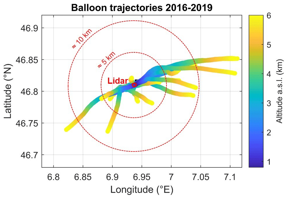
Figure 1 Balloon trajectories (longitude vs. latitude) as a function of altitude (color scale) for all the analyzed soundings of the RALMO vs. COBALD comparison (17 profiles, 2016–2019). The trajectories are plotted with a vertical resolution of 30 m between 0.8–6 km altitude a.s.l. The location of the RALMO and CHM15K lidars (and balloon launching site) is shown by the solid red circle (46.82^∘ E, 6.95^∘ N). The two dotted red circles indicate horizontal distances of approximately 5 and 10 km from the lidar site.

In addition, the two techniques differ in terms of measurement times. Namely, while the lidar profiles are integrated 30 min in time, COBALD provides instantaneous measurements at 1 s resolution (reduced to 6 s after averaging to 30 m intervals). The combination of balloon drift with altitude and different integration times, coupled with the high spatial and temporal variability in aerosol optical properties, can lead to discrepancies between the remote-sensing and in situ measurement which are not due to instrumental issues but rather to atmospheric-variability effects. In particular, this may result in the smoothing or slight displacement in altitude between aerosol backscatter features (especially thin layers), which are seen by both techniques. Such effects are often observed in our dataset and therefore affect the results of the statistical comparison. This issue is discussed further in Sect. 4.3.

3 Method of comparison

For each COBALD sounding, we retrieve simultaneous RALMO and CHM15K β_aer profiles with a vertical resolution of 30 m and integration time of 30 min (roughly corresponding to 10 km of balloon ascent time). Since all COBALD sondes were launched at 23:00 UTC, the integration time window chosen for all profiles and both lidars is 23:00–23:30 UTC. To obtain a dataset with consistent vertical levels, the COBALD measurements (with a vertical resolution ≈ 5 m) are averaged in altitude bins of 30 m, matching the vertical grid of the lidars. For the statistical comparison we consider in total 174 vertical levels, covering the altitude interval from 800 m a.s.l. to 6 km a.s.l. We only select measurements from ≈ 300 m above the ground station to avoid the region of maximum incomplete overlap of CHM15K as well as to avoid the region of low signal-to-noise ratio of RALMO at low altitudes (see Sect. 2.1). Note that all altitude levels given in the following are meant as altitude a.s.l. unless differently specified.

Along with the COBALD backscatter data, the temperature, pressure and relative humidity (RH) measurements from the host radiosonde are averaged to the same altitude levels. The temperature and pressure profiles are used for the computation of the atmospheric molecular extinction, as described in Sect. 2.2. The RH measurements are used to reject in-cloud data points. In-cloud aerosol backscatter measurements are typically much larger (up to 3 orders of magnitude) compared to clear-sky (i.e., aerosol-only) conditions and characterized by high spatial and temporal variability. Therefore, we exclude from the comparison all data points with RH > 90 %. Such a highly conservative criterion is chosen in order to avoid cloud edge regions as well, which can lead to large biases in the statistical comparison.

For a proper comparison of the COBALD and lidar backscatter retrievals, a number of methodological aspects and technical differences between the two techniques need to be taken into account. In the remainder of this section, we discuss our approach towards wavelength homogenization (Sect. 3.1), correction of effects related to the different receiver FOVs (Sect. 3.2), data sorting according to aerosol content and compared quantities (Sect. 3.3).

3.1 Wavelength conversion

To compare β_aer at different wavelengths (λ) measured by the different instruments, it is necessary to account for the spectral dependency of aerosol backscatter. This is done using the Ångström law (Eq. 2), which describes the spectral dependency of β_aer between two wavelengths (λ₀ and λ) as a function of the Ångström exponent (AE) at every altitude level (z_i). The AE is an intensive property of the aerosol that, under certain assumptions on the particle's size distribution, can be used as a semi-quantitative indicator of particle size (e.g., Njeki et al., 2012; Navas-Guzmán et al., 2019). Through Eq. (2) we convert the lidar profiles into the COBALD wavelengths so they can be quantitatively compared.

$$\begin{array}{}\text{(2)}& {\mathit{\beta }}_{\mathrm{aer}}\left(\mathit{\lambda },z_i\right)={\mathit{\beta }}_{\mathrm{aer}}\left({\mathit{\lambda }}_{\mathrm{0}},z_i\right)\cdot {\left({\displaystyle \frac{\mathit{\lambda }}{{\mathit{\lambda }}_{\mathrm{0}}}}\right)}^{-\mathrm{AE}\left(z_i\right)}\end{array}$$

Thanks to its high signal-to-noise ratio and two operating wavelengths, COBALD allows us to characterize the backscatter spectral ratio (between 455 and 940 nm) at every altitude, including regions of low aerosol load (e.g., Brunamonti et al., 2018). Conversely, the signal-to-noise ratio of remote-sensing instruments (in our case especially CHM15K) decreases with altitude, and the AE derived from lidar measurements is typically characterized by large statistical fluctuations in the free troposphere. Therefore, here we choose to retrieve the AE(z) profiles from COBALD data. To minimize the uncertainty associated with the conversion, we couple each lidar with the closest COBALD channel in terms of wavelength. Hence, the RALMO profiles at 355 nm (ultraviolet) are converted to 455 nm and compared to the COBALD blue visible channel, and the CHM15K profiles at 1064 nm (infrared) are converted to 940 nm and compared to the COBALD infrared channel.

Using the AE from COBALD is equivalent to assuming that the spectral behavior of the aerosols between 455–940 nm can be extrapolated to the slightly broader interval of 355–1064 nm, which is justified by the small difference between the wavelengths that are compared. A number of sensitivity tests using different assumptions have been conducted, revealing that small changes in AE have a small effect on the results. The uncertainty associated with the wavelength conversion of the lidar data is discussed further in Sect. 4.3.

3.2 FOV correction

Besides their wavelengths, the COBALD and lidar systems differ in terms of FOV of their respective receivers. RALMO and CHM15K use highly focused laser beams and consequently have narrow FOVs (200 and 450 µrad, respectively, corresponding to 0.01–0.02^∘), while COBALD's photodiode detector has a macroscopic FOV of 6^∘ (see Table 1). Considering that the Mie-scattering phase function, i.e., the distribution of scattered light with angle by a spherical particle, has a local maximum in the backward direction (180^∘), it follows from its wider FOV that COBALD will measure less backscattered radiation (namely, the average intensity between 174–180^∘) compared to the lidars (≈ 180^∘).

To quantify this effect, we performed idealized Mie-theory scattering simulations using the optical model by Luo et al. (2003). We assume a single lognormal size distribution of aerosol particles characterized by mode radius R_m, number concentration N, fixed width (standard deviation 1.4) and refractive index (1.4). The BSR of this population is then computed both assuming the phase function value at 180^∘, corresponding to the lidar observations (FOV ≈ 0^∘), and taking the average of the phase function between angles 174–180^∘, corresponding to the COBALD measurements (FOV = 6^∘). The use of a mono-modal size distribution with fixed width has the advantage that the correction factors can be described as functions of a single parameter (R_m), which can be constrained through the observed AE. Furthermore, a mono-modal distribution represents well the average size distribution of continental aerosols in the northern mid-latitudes (e.g., Watson-Perris et al., 2019).

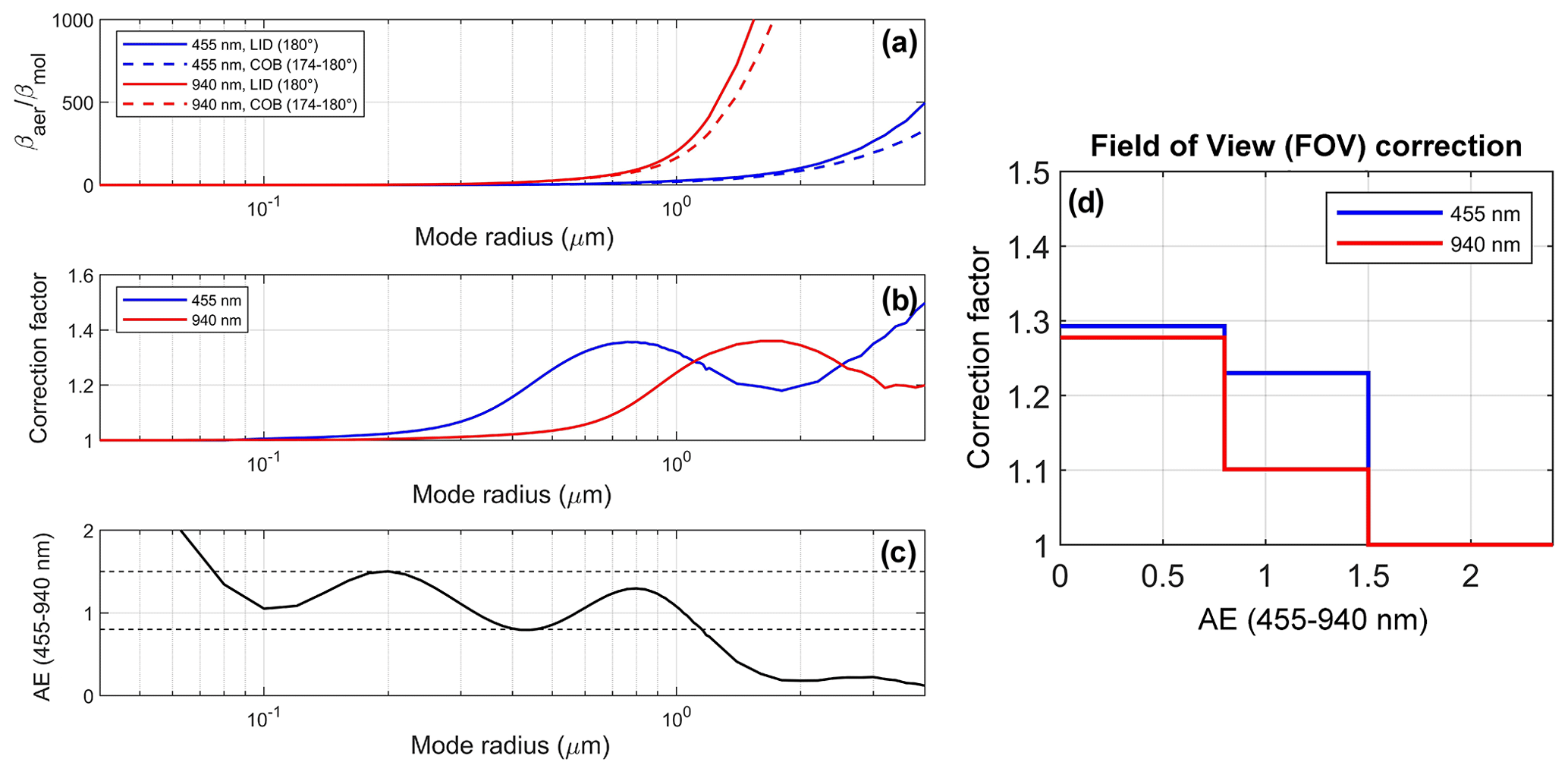
Figure 2 Mie-theory scattering model simulations. Panel (a): ratio of aerosol-to-molecular-backscatter coefficient, ${\mathit{\beta }}_{\mathrm{aer}}/{\mathit{\beta }}_{\mathrm{mol}}$ (i.e., BSR −1) at 455 nm (blue) and 940 nm (red), as a function of mode radius (R_m), calculated assuming a FOV angle of 174–180^∘ (dashed lines: COBALD) and 180^∘ (solid lines: lidar), and aerosol number concentration N= 10³ cm⁻³. Panel (b): correction factors, i.e., lidar-to-COBALD ratio of ${\mathit{\beta }}_{\mathrm{aer}}/{\mathit{\beta }}_{\mathrm{mol}}$ (as shown in panel a) for 455 nm (blue) and 940 nm (red), as a function of R_m. Panel (c): simulated Ångström exponent (AE) for the COBALD wavelength interval (455–940 nm), as a function of R_m. Dashed black lines indicate the thresholds of AE = 0.8 and AE = 1.5 used for the parameterization of the correction factors (see Sect. 3.2). Panel (d): resulting FOV correction as a function of AE.

Figure 2a shows the simulated ratio of aerosol-to-molecular-backscatter coefficient, ${\mathit{\beta }}_{\mathrm{aer}}/{\mathit{\beta }}_{\mathrm{mol}}$ (i.e., BSR – 1; see Eq. 1) at 455 nm (blue) and 940 nm (red), as a function of R_m (40 nm–4 µm), calculated assuming FOV ≈ 0^∘ (solid lines) and FOV = 6^∘ (dashed lines), and N= 10³ cm⁻³. As expected, the simulations show that for all mode radii the COBALD β_aer is lower than the β_aer measured by the lidar instruments. Figure 2b shows the lidar-to-COBALD ratio of β_aer (ratio of solid-to-dashed curves in Fig. 2a), i.e., the correction factor required to compensate for the FOV effect, for 455 and 940 nm as a function of R_m. For the considered size interval, the correction factors vary between approximately 1–1.5 and show a non-linear dependency on R_m, with a local maximum near 800 nm (λ= 455 nm) and 1.6 µm (λ= 940 nm). This complex optical behavior needs to be corrected. Note that the correction factors in Fig. 2b are independent of N, unlike the ${\mathit{\beta }}_{\mathrm{aer}}/{\mathit{\beta }}_{\mathrm{mol}}$ ratios in Fig. 2a.

To account for the size dependency in Fig. 2b, we use the AE as an indicator of particle size and develop a parametrization of the correction factors based on the AE measured from COBALD. Figure 2c shows AE between 455–950 nm calculated from the Mie simulations as a function of R_m. The AE decreases non-monotonically with mode radius and exhibits the characteristic Mie oscillations in the range of approximately 40 nm–1 µm (Fig. 2c). More in detail, we observe that AE > 1.5 corresponds to small particles (R_m < 75 nm) and AE < 0.8 to large particles (R_m > 1.16 µm), while 0.8 < AE < 1.5 corresponds to 75 nm < R_m < 1.16 µm, but in this intermediate range the change in AE with R_m is not monotonic (Fig. 2c); hence a one-to-one correspondence cannot be established. To simplify this behavior, we parametrize the correction factors within the three fixed intervals of AE just introduced, and for each interval of AE we take the average correction factor in the corresponding interval of R_m. Hence, we apply the average correction factors between 75 nm–1.16 µm (namely, 1.23 at 455 nm, 1.10 at 940 nm) to all measurements with 0.8 < AE < 1.5, the average correction factors between 1.16–4 µm (1.29 at 455 nm, 1.28 at 940 nm) for AE < 0.8, and no correction for AE > 1.5 (both correction factors ≈ 1 for R_m < 75 nm). The resulting FOV correction as a function of AE is shown in Fig. 2d.

The FOV correction is applied to all COBALD measurements in the statistical comparison. Since, for every AE, the correction factors are larger for 455 nm than for 940 nm (Fig. 2d), the FOV correction will affect the RALMO comparison more than the CHM15K one. We note that, due to the variability in AE observed in our dataset (see Fig. S1 in the Supplement), the middle interval of the correction (0.8 < AE < 1.5) accounts for the large majority of data points in the PBL, and AE > 1.5 typically corresponds to free-tropospheric background measurements, which are unaffected by the correction, while values of AE < 0.8, corresponding to very large particles, are rarely encountered in our dataset. The effect of the FOV correction on two selected profiles is discussed in Sect. 4.1.

3.3 Compared quantities

After the wavelength conversion and the FOV correction, the difference in aerosol backscatter coefficient (Δβ_aer) between the lidars (LIDs) and COBALD (COB) is calculated for each sounding and every altitude level as in Eq. (3). The mean deviation (δ) of a given subset of data is calculated according to Eq. (4), where z₁ … z_N is the ensemble of all vertical levels in the considered dataset and altitude region. The spread of the individual differences around δ is quantified using standard deviation (σ), defined by Eq. (5). Δβ_aer, δ and σ are expressed in both absolute backscatter coefficient values (Mm⁻¹ sr⁻¹) and percent units relative to the COBALD signal (denoted as $\mathrm{\Delta }{\mathit{\beta }}_{\mathrm{aer}}^{\mathrm{rel}}{\mathit{\delta }}_{\mathrm{rel}},{\mathit{\sigma }}_{\mathrm{rel}}$).

$$\begin{array}{}\text{(3)}& {\displaystyle }\mathrm{\Delta }{\mathit{\beta }}_{\mathrm{aer}}\left(z_i\right)={\mathit{\beta }}_{\mathrm{aer}}^{\mathrm{LID}}\left(z_i\right)-{\mathit{\beta }}_{\mathrm{aer}}^{\mathrm{COB}}\left(z_i\right)\text{(4)}& {\displaystyle }\mathit{\delta }={\displaystyle \frac{{\sum }_{i=\mathrm{1}}^N\mathrm{\Delta }{\mathit{\beta }}_{\mathrm{aer}}\left(z_i\right)}{N}}\text{(5)}& {\displaystyle }\mathit{\sigma }=\sqrt{{\displaystyle \frac{{\sum }_{i=\mathrm{1}}^N\left(\mathrm{\Delta }{\mathit{\beta }}_{\mathrm{aer}}\right(z_i)-\mathit{\delta }{)}^{\mathrm{2}}}{N-\mathrm{1}}}}\end{array}$$

Atmospheric backscatter profiles are typically characterized by a large gradient in β_aer between the boundary layer, with high aerosol content (hence high β_aer), and the free troposphere, with low aerosol content (low β_aer). This gradient is such that the same absolute Δβ_aer may correspond to either a small or large relative $\mathrm{\Delta }{\mathit{\beta }}_{\mathrm{aer}}^{\mathrm{rel}}$, depending on altitude. In particular, free-tropospheric measurements, where statistical fluctuations often dominate over the atmospheric signal, typically yield large relative deviations in spite of small absolute differences. While the boundary layer is the main region of the interest of this study as it contains most of the aerosol loading in the column, the free troposphere (including low-aerosol-content measurement) cannot be completely neglected since a good agreement at high altitudes ensures that all profiles are well calibrated (see Sect. 2.3). Therefore, here we focus our analysis on medium-high-aerosol-content data (defined as explained below), yet for completeness we also display low-aerosol-content measurements in the statistical comparison.

The aerosol content is evaluated according to the average COBALD β_aer in each profile and 300 m altitude interval (i.e., mean of 10 vertical levels). Based on the observed range of variability in β_aer in our dataset (see Fig. S1), we define “low aerosol content” as all layers with average COBALD β_aer < 0.1 Mm⁻¹ sr⁻¹ at 455 nm (RALMO comparison) and average COBALD β_aer < 0.05 Mm⁻¹ sr⁻¹ at 940 nm (CHM15K comparison). The averaging in 300 m layers ensures that actual air masses with low aerosol content are identified rather than individual data points exceeding the threshold due to statistical variability. When the above conditions are met, all data points in the considered layer are classified as “low aerosol content”. All other data points are referred to as “medium-high aerosol content”. Note that this definition allows individual data points to exceed the threshold as long as the average criteria in the layer are not exceeded.

For medium-high-aerosol-content data, in addition to δ and σ, we also evaluate the correlation between the lidars and COBALD using the Pearson correlation coefficient (ρ). This is defined according to Eq. 6, where B_LID and B_COB are the average lidar β_aer and COBALD β_aer, respectively, calculated in 300 m layers. The Pearson correlation coefficient represents the degree of linearity of the correlation between ${\mathit{\beta }}_{\mathrm{aer}}^{\mathrm{LID}}$ and ${\mathit{\beta }}_{\mathrm{aer}}^{\mathrm{COB}}$, ranging between values of −1 (total negative linear correlation) and +1 (total positive linear correlation). In the statistical comparison, δ, σ and ρ are quantified for both RALMO and CHM15K in three altitude intervals of 0.8–3, 3–6 and 0.8–6 km a.s.l. (i.e., all altitudes).

$$\begin{array}{}\text{(6)}& \mathit{\rho }={\displaystyle \frac{{\sum }_{i=\mathrm{1}}^N\left({\mathit{\beta }}_{\mathrm{aer}}^{\mathrm{LID}}\left(z_i\right)-B_{\mathrm{LID}}\right)\cdot \left({\mathit{\beta }}_{\mathrm{aer}}^{\mathrm{COB}}\left(z_i\right)-B_{\mathrm{COB}}\right)}{\sqrt{{\sum }_{j=\mathrm{1}}^N{\left({\mathit{\beta }}_{\mathrm{aer}}^{\mathrm{LID}}\left(z_i\right)-B_{\mathrm{LID}}\right)}^{\mathrm{2}}\cdot {\sum }_{k=\mathrm{1}}^N{\left({\mathit{\beta }}_{\mathrm{aer}}^{\mathrm{COB}}\left(z_i\right)-B_{\mathrm{COB}}\right)}^{\mathrm{2}}}}}\end{array}$$

4 Results

In this section we present the results of our analysis. Before the statistical comparison (Sect. 4.2), we discuss the comparison of two selected individual profiles (Sect. 4.1), highlighting the effect of the FOV correction. Finally, the results are discussed in Sect. 4.3. Two additional examples of individual profiles can be found in the Supplement (Figs. S2–S3).

4.1 Comparison of individual profiles

To illustrate the main characteristics of the observed β_aer profiles and the effect of the FOV correction, we select as case studies the soundings performed on 12 July and 4 September 2018. Figure 3 shows an overview of these measurements – including vertical profiles of β_aer (at different λ) by RALMO, COBALD and CHM15K (panels a, d), AE derived from COBALD measurements (panels b, e), and the temperature and RH profiles measured by the radiosonde (panels c, f) – as functions of altitude for the interval of 0.8–6 km a.s.l.

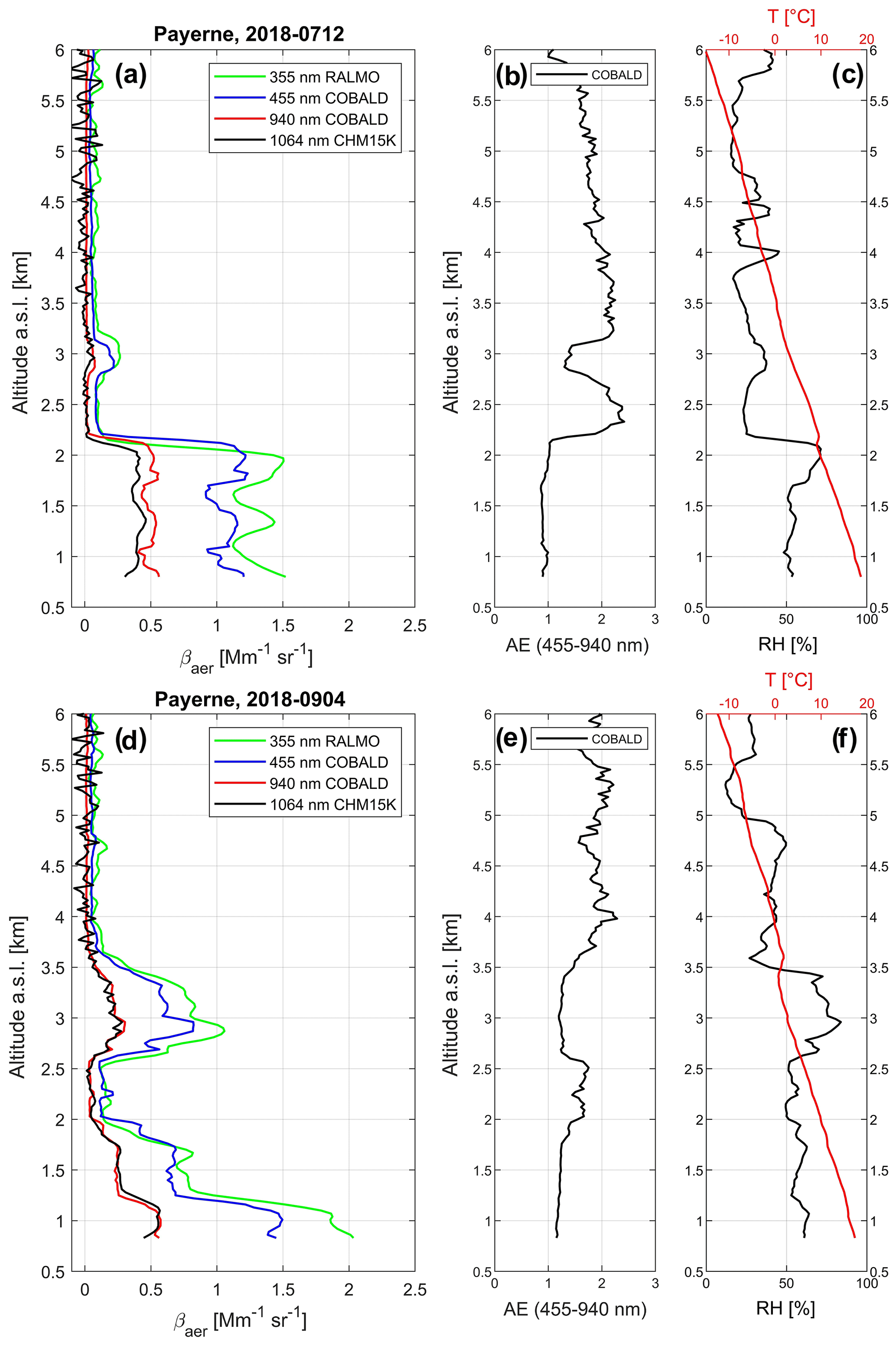
Figure 3 Overview of selected profiles measured on 7 July 2018 (a–c) and 4 September 2018 (d–f). Panels (a, c): vertical profiles of aerosol backscatter coefficient (β_aer) as a function of altitude, measured by RALMO (355 nm: green), COBALD (455 nm: blue; 940 nm: red) and CHM15K (1064 nm: black). Panels (b, d): vertical profiles of Ångström exponent (AE) for wavelengths 455–940 nm, calculated from the COBALD data. Panels (c, f): vertical profiles of relative humidity (RH: black) and temperature (red, top scale) measured by the Vaisala RS41-SGP radiosonde (flying in tandem with the COBALD sonde).

The case of 12 July 2018 (Fig. 3a–c) shows a typical profile with top of PBL at about 2.2 km altitude (see temperature inversion in panel c), characterized by a sharp decrease with altitude in β_aer and RH, plus a thin (≈ 400 m) isolated aerosol layer around 3 km altitude (note the higher AE compared to the PBL, suggesting finer particles; panel b). Inside the PBL, the vertical structure of β_aer observed by COBALD is qualitatively well reproduced by both RALMO and CHM15K, despite an evident altitude displacement (of about 60 m) of the top-of-PBL decrease in β_aer between the COBALD and lidar profiles (Fig. 3a). This is most likely an effect of the atmospheric-variability issues discussed in Sect. 2.4. Indeed, considering that COBALD crosses the PBL around the beginning of the lidar integration time window, a downward displacement in top-of-PBL altitude (as inferred from the β_aer profiles) in the remote-sensing data is consistent with the lowering of PBL altitude during nighttime reported by Poltera et al. (2017). A similar feature can be seen in Fig. S2d.

On 4 September 2018 (Fig. 3d–f) a more complex aerosol vertical distribution is observed, with decreasing β_aer with altitude until 2 km and a thick aerosol layer between 2.5–3.5 km altitude. Again, the vertical structure of β_aer observed by COBALD is very well reproduced by both remote-sensing products throughout the entire analyzed altitude range, including both aerosol layers inside and above the PBL. In this case, no significant altitude displacement is observed between the β_aer features of the COBALD and remote-sensing profiles (Fig. 3d).

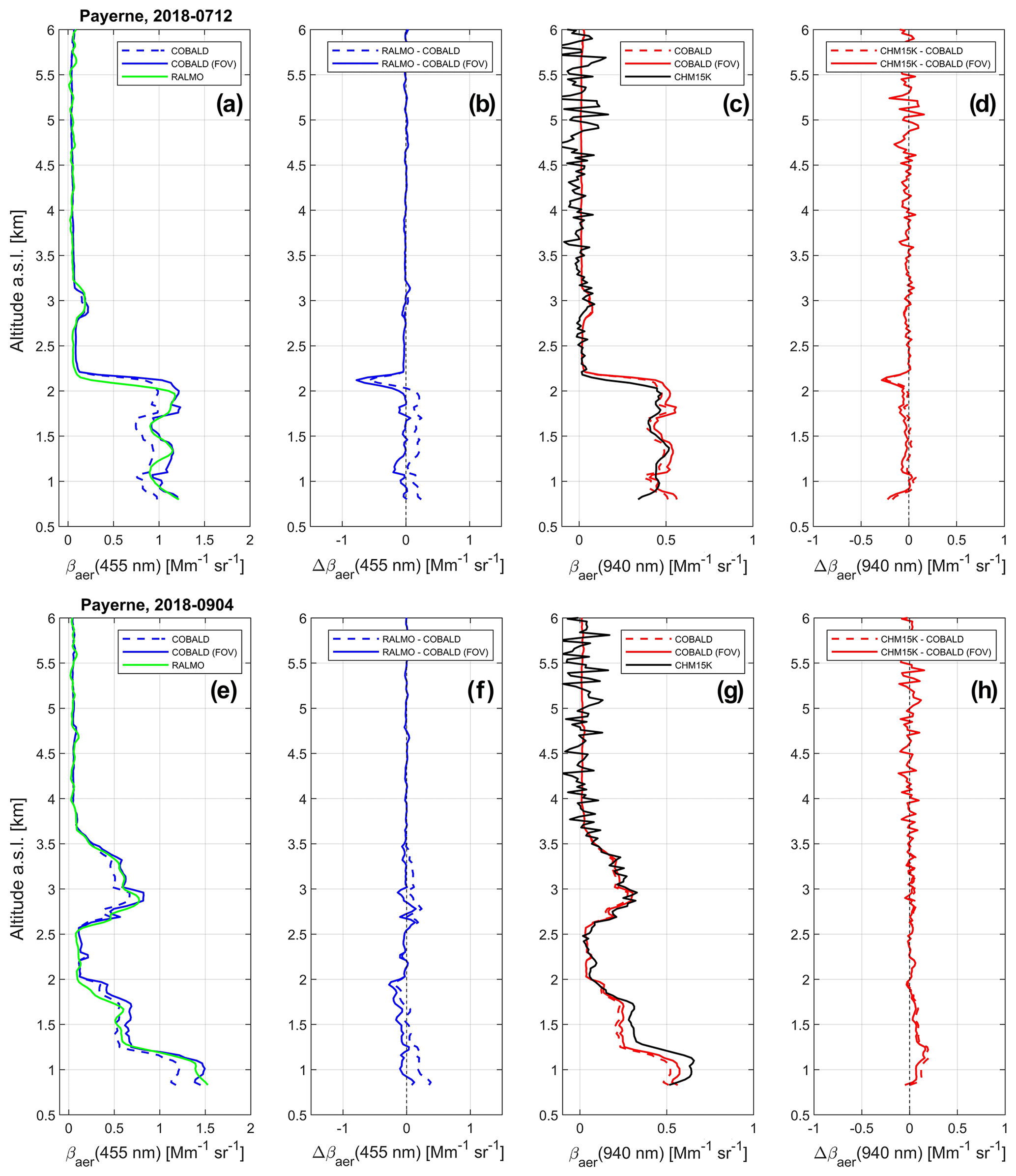
Figure 4 Quantitative comparison of RALMO vs. COBALD (a–b, e–f) and CHM15K vs. COBALD (c–d, g–h) for the selected profiles measured on 7 July 2018 (a–d) and 4 September 2018 (e–h). Panels (a, e): vertical profiles of aerosol backscatter coefficient (β_aer) at 455 nm measured by RALMO (green) and COBALD (blue), both without (dashed) and with (solid) application of the FOV correction. Panels (b, f): vertical profiles of the RALMO−COBALD difference in β_aer (Δβ_aer) at 455 nm, both without (dashed) and with (solid) application of the FOV correction. Panels (c, g): vertical profiles of β_aer at 940 nm measured by CHM15K (black) and COBALD (red), both without (dashed) and with (solid) FOV correction. Panels (d, h): vertical profiles of Δβ_aer for CHM15K−COBALD at 940 nm, both without (dashed) and with (solid) FOV correction.

Figure 4 shows the results of the quantitative comparison for the two cases just discussed, meaning the β_aer profiles obtained after converting the lidar wavelengths (355 to 455 nm and 1064 to 940 nm) and applying the FOV correction to the COBALD measurements. In particular, Fig. 4 shows vertical profiles of β_aer at 455 nm from RALMO and COBALD (panels a, e), β_aer at 940 nm from CHM15K and COBALD (panels c, g), and their respective differences (Δβ_aer) at 455 nm (panels b, f) and 940 nm (panels d, h) for 12 July 2018 (panels a–d) and 4 September 2018 (panels e–h). The COBALD β_aer and Δβ_aer profiles are shown both before (dashed lines) and after (solid lines) the FOV correction.

The FOV correction significantly improves the agreement between RALMO and COBALD measurements. Before the correction (dashed lines), the RALMO profiles are characterized by a systematic high bias with respect to COBALD of about 0.2 Mm⁻¹ sr⁻¹ in the PBL (Fig. 4a–b, e–f). After the FOV correction (solid lines), which increases the COBALD β_aer by a factor of 1.23 in this region of altitudes (see Fig. 2d and AE profiles in Fig. 3b), the discrepancy with RALMO is drastically reduced, and the profiles are in good agreement within ±0.1 Mm⁻¹ sr⁻¹ (Fig. 4b, f). In relative terms, this corresponds to deviations of less than 10 % of the observed signal in the PBL, which is comparable to the estimated statistical uncertainty associated with the remote-sensing measurements alone (see Sect. 2.1).

As already noted in Sect. 3.2, the effect of the FOV correction on the CHM15K comparison is smaller. In particular, for the case of 4 September 2018 (Fig. 4g–h) the correction leads to a slight improvement in agreement with COBALD (≈ 0.05 Mm⁻¹ sr⁻¹), whereas on 12 July 2018 (Fig. 4c–d) it slightly increases the discrepancy. Due to the empirical implementation of the FOV correction, with many assumptions and simplifications involved (e.g., single-mode size distribution, coarse parameterization in AE space), it is to be expected that for individual sounding the magnitude of the correction might be underestimating or overestimating the true effect of the different FOVs. The uncertainty introduced by the FOV correction in the statistical comparison is discussed more in detail in Sect. 4.3.

4.2 Statistical comparison

Here we present the results of the statistical comparison for the dataset introduced in Sect. 2.3, consisting of 17 simultaneous RALMO vs. COBALD profiles (Sect. 4.2.1) and 31 CHM15K vs. COBALD profiles (Sect. 4.2.2).

4.2.1 RALMO vs. COBALD

Figure 5 shows all data points of the RALMO−COBALD difference (Δβ_aer at 455 nm) as a function of altitude, expressed in both absolute backscatter coefficient units (panel a) and percent units relative to the COBALD signal (panel b), after the FOV correction was applied to all COBALD measurements. Medium-high- and low-aerosol-content measurements, classified as in Sect. 3.3, are shown by dark-blue and light-blue circles, respectively. The mean deviation (δ) and mean ± standard deviation (δ ± σ) profiles of medium-high-aerosol-content data are shown in both panels as thick and thin solid black lines, respectively. As discussed in Sect. 3, to avoid in-cloud measurements, we only consider data points with RH < 90 % (according to the radiosonde measurements).

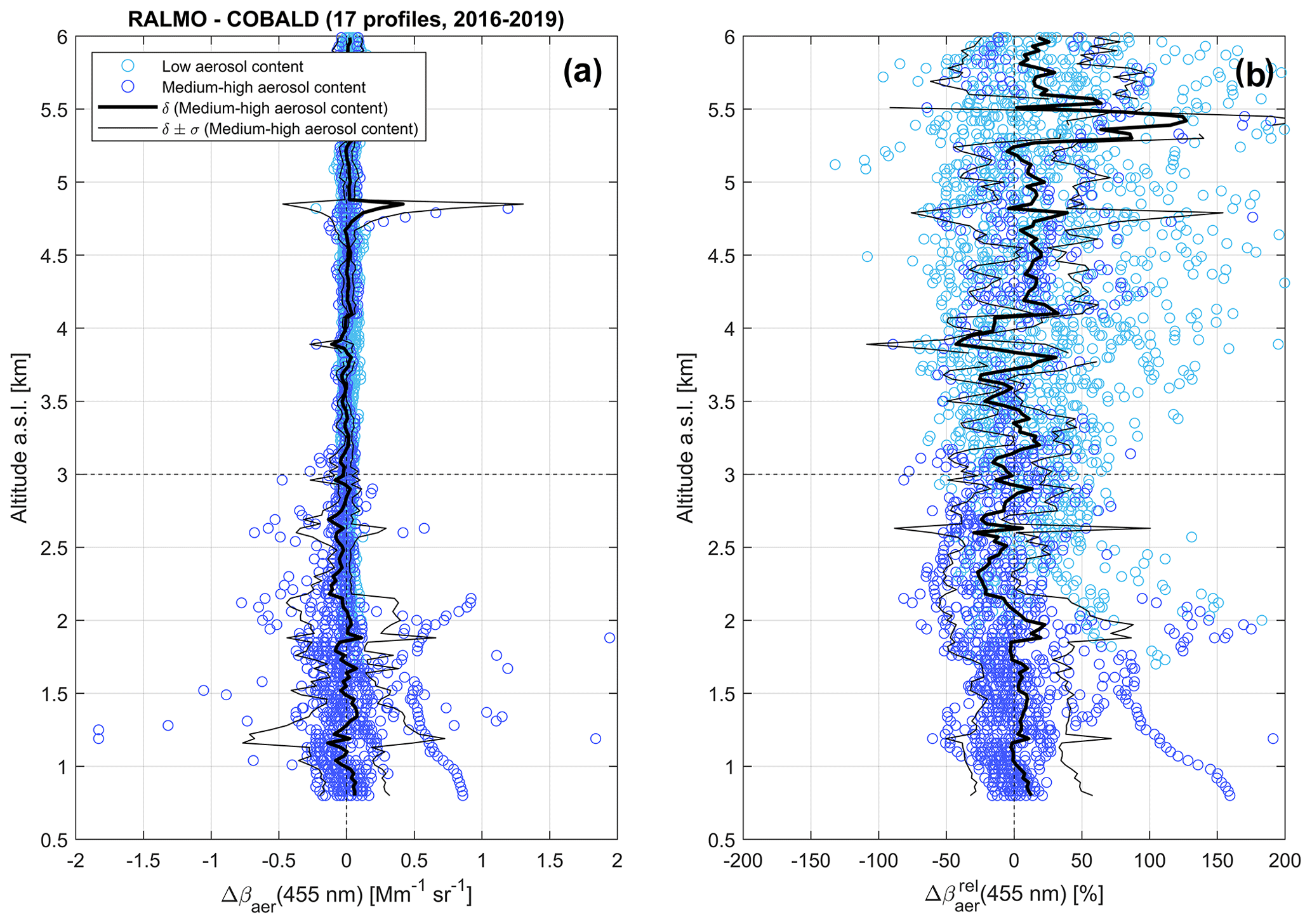
Figure 5 Statistical comparison of RALMO vs. COBALD: vertical profiles. Panel (a): all medium-high-aerosol-content (dark-blue circles) and low-aerosol-content (light-blue circles) data points of the RALMO−COBALD aerosol backscatter coefficient difference (Δβ_aer) at 455 nm as a function of altitude. Panel (b): same as panel (a), with Δβ_aer expressed in percent units (%) relative to the COBALD measurements (i.e., $\mathrm{\Delta }{\mathit{\beta }}_{\mathrm{aer}}^{\mathrm{rel}}$). Mean deviation (δ) and mean ± standard deviation (δ ± σ) profiles are shown in both panels by thick solid and thin dashed black lines, respectively. The 3 km altitude level is highlighted by a thin dashed black line.

Medium-high-aerosol-content measurements of RALMO and COBALD β_aer are on average in good agreement over the entire altitude range (0.8–6 km a.s.l.), yet significant discrepancies can occur in individual profiles. As expected, the largest absolute differences are observed at low altitudes (z < 3 km), including most of the PBL (hence medium-high-aerosol-content) measurements in our dataset (Fig. 5a). Conversely, smaller absolute discrepancies yet large relative differences (Fig. 5b) are found in the free troposphere (z > 3 km), where low-aerosol-content measurements prevail.

For z < 3 km, the mean deviation profile (δ) of medium-high-aerosol-content data stays within ±0.1 Mm⁻¹ sr⁻¹, while standard deviation (σ) ranges between 0.1–0.4 Mm⁻¹ sr⁻¹, and individual data points rarely exceed ± 0.5 Mm⁻¹ sr⁻¹ (Fig. 5a). In relative terms, δ_rel shows an average slight overestimation of 5 %–10 % below 2 km (with σ_rel≈ 40 %) and an underestimation of 10 %–25 % between 2–3 km (σ_rel≈ 30 %) (Fig. 5b). Such large relative standard deviations can be at least partly attributed to the uncertainties associated with the wavelength conversion and FOV correction of the data (Sect. 3.1–3.2) and spatial- and temporal-variability effects (Sect. 2.4). These issues are discussed in more detail in Sect. 4.3. For z > 3 km, nearly all absolute differences are smaller than ±0.1 Mm⁻¹ sr⁻¹ (Fig. 5a). Medium-high-aerosol-content data points above 3 km altitude generally stay within deviations of ±50 %, whereas low-aerosol-content ones often exceed ±100 % (Fig. 5b).

Figure 6 shows the frequency-of-occurrence distribution of RALMO−COBALD Δβ_aer, calculated for the altitude intervals of 0.8–3 km (panels a–b), 3–6 km (panels c–d) and 0.8–6 km (i.e., all altitudes: panels e–f), for medium-high-aerosol-content data (blue bars) and all data (i.e., including low aerosol content: black lines). The distributions are calculated in both absolute units within 40 intervals of 0.1 Mm⁻¹ sr⁻¹ width between ±2 Mm⁻¹ sr⁻¹ (panels a, c, e), and relative units within 40 intervals of 10 % width between ±200 % (panels b, d, f).

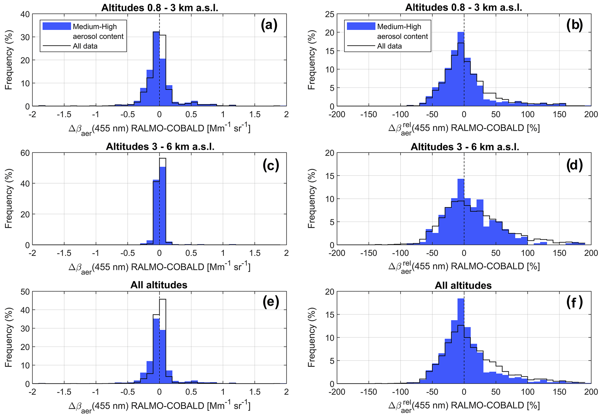
Figure 6 Statistical comparison of RALMO vs. COBALD: frequency-of-occurrence distributions of medium-high-aerosol-content data (blue bars) and all data (black lines). Panels (a, c, e): frequency-of-occurrence distributions of the RALMO−COBALD difference in aerosol backscatter coefficient (Δβ_aer) at 455 nm for the altitude intervals 0.8–3 km a.s.l. (a), 3–6 km a.s.l. (c) and 0.8–6 km a.s.l. (i.e., all altitudes: panel e). Panels (b, d, f): same as panels (a, c, e), with Δβ_aer expressed in percent units (%) relative to the COBALD measurements (i.e., $\mathrm{\Delta }{\mathit{\beta }}_{\mathrm{aer}}^{\mathrm{rel}}$). The frequency-of-occurrence distributions are calculated in Δβ_aer intervals of 0.1 Mm⁻¹ sr⁻¹ (a, c, e) and 10 % (a, c, e).

In all distributions, medium-high-aerosol-content measurements show a higher frequency of occurrence of small relative deviations compared to all data (Fig. 6b, d, f) and a lower frequency of occurrence of small absolute differences (Fig. 6b, d, f). The absolute (relative) δ ± σ for medium-high-aerosol-content data is −0.018 ± 0.237 Mm⁻¹ sr⁻¹ (−2 % ± 37 %) for altitudes 0.8–3 km, +0.015 ± 0.068 Mm⁻¹ sr⁻¹ (+13 % ± 38 %) for 3–6 km and +0.001 ± 0.141 Mm⁻¹ sr⁻¹ (+6 % ± 38 %) for all altitudes (see Table 2). Considering all data, δ_rel ± σ_rel increases to +5 % ± 40 % for 0.8–3 km, +19 % ± 53 % for 3–6 km and +13 % ± 47 % for all altitudes. We observe that the skewness of the medium-high-aerosol-content distribution for 0.8–3 km (Fig. 6a–b) is strongly influenced by a single strongly outlying profile, showing $\mathrm{\Delta }{\mathit{\beta }}_{\mathrm{aer}}^{\mathrm{rel}}$ > 100 % at z < 2 km (see Fig. 5b), which is likely related to atmospheric-variability effects (see discussion in Sect. 4.3).

Table 2 Statistical comparison of RALMO vs. COBALD: results for medium-high aerosol content. For each altitude interval, we show mean deviation (in both absolute units, δ, and percent units relative to COBALD, δ_rel) and standard deviation (in both absolute units, σ, and percent units relative to COBALD, σ_rel) at 455 nm as well as Pearson correlation coefficient (ρ).

Finally, to evaluate their correlation, Fig. 7 shows a scatterplot of all RALMO vs. COBALD measurements of β_aer at 455 nm (between 0.03–5 Mm⁻¹ sr⁻¹). As in Fig. 5, medium-high-aerosol-content data are shown as dark-blue circles and low-aerosol-content data as light-blue circles. Isolines of Δβ_aer= 0, $\mathrm{\Delta }{\mathit{\beta }}_{\mathrm{aer}}^{\mathrm{rel}}=$ ±25 % and $\mathrm{\Delta }{\mathit{\beta }}_{\mathrm{aer}}^{\mathrm{rel}}=$ ±50 % differences are indicated by solid, dashed and dotted black lines, respectively. The 0.1 Mm⁻¹ sr⁻¹ threshold in COBALD β_aer at 455 nm, separating low- from medium-high-aerosol-content layers as described Sect. 3.3, is also shown as a thin dashed vertical line.

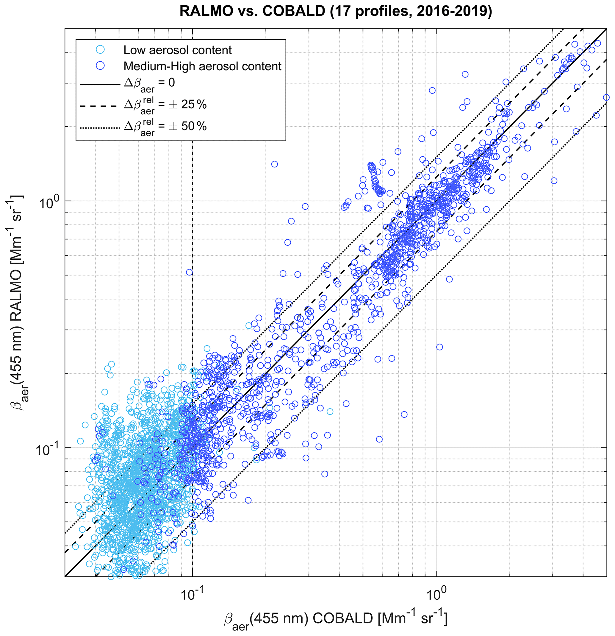
Figure 7 Statistical comparison of RALMO vs. COBALD: scatterplot. All medium-high-aerosol-content (dark-blue circles) and low-aerosol-content (light-blue circles) data points of aerosol backscatter coefficient (β_aer) at 455 nm measured by RALMO (y axis) vs. β_aer at 455 nm measured by COBALD (x axis). Thin black lines show 1:1 agreement (solid), ±25 % difference (dashed) and ±50 % difference (dotted) isolines. The 0.1 Mm⁻¹ sr⁻¹ threshold in COBALD β_aer, separating low- from medium-high-aerosol-content data at 455 nm (as described in Sect. 3.3), is shown by a dashed vertical black line.

Figure 7 shows a good correlation between RALMO and COBALD measurements in medium-high-aerosol-content conditions and, as expected, a larger spread for low-aerosol-content data. The Pearson correlation coefficient (ρ) of medium-high-aerosol-content data is +0.81 for altitudes 0.8–3 km, +0.62 for 3–6 km and +0.80 for all altitudes (see Table 2), indicating a high degree of linear correlation between RALMO and COBALD measurements up to 6 km. We note from Fig. 7 that the highest density of medium-high-aerosol-content measurements is found at β_aer ≈ 0.4–2 Mm⁻¹ sr⁻¹, suggesting that this interval represents the average PBL aerosol content in our dataset. Here, RALMO and COBALD show a particularly good agreement, with most individual differences staying below ±25 % (Fig. 7).

4.2.2 CHM15K vs. COBALD

Following the same structure of the previous subsection, here we analyze the CHM15K vs. COBALD statistical comparison first in terms of vertical profiles (Fig. 8), then frequency-of-occurrence distributions (Fig. 9) and finally a scatterplot of all CHM15K vs. COBALD measurements (Fig. 10).

Figure 8 Statistical comparison of CHM15K vs. COBALD: vertical profiles. Panel (a): all medium-high-aerosol-content (red circles) and low-aerosol-content (orange circles) data points of CHM15K−COBALD aerosol backscatter coefficient difference (Δβ_aer) at 940 nm as a function of altitude. Panel (b): same as panel (a), with Δβ_aer expressed in percent units (%) relative to the COBALD measurements (i.e., $\mathrm{\Delta }{\mathit{\beta }}_{\mathrm{aer}}^{\mathrm{rel}}$). Mean deviation (δ) and mean ± standard deviation (δ ± σ) profiles are shown in both panels by thick solid and thin dashed black lines, respectively. The 3 km altitude level is highlighted by a thin dashed black line.

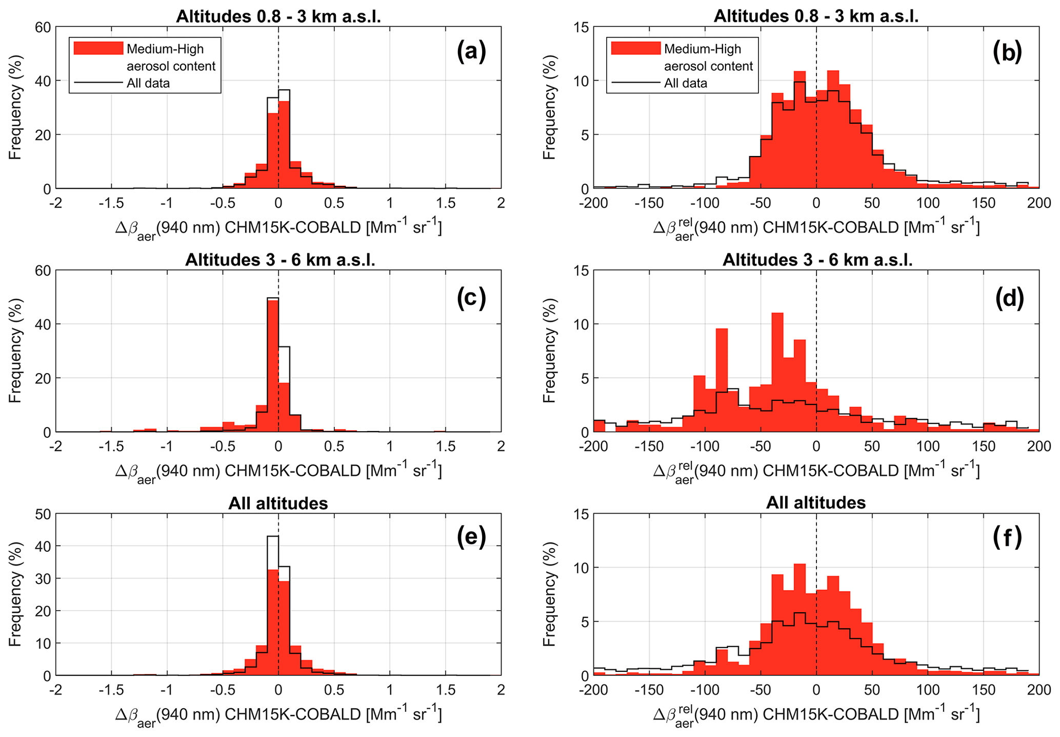
Figure 9 Statistical comparison of CHM15K vs. COBALD: frequency-of-occurrence distributions of medium-high-aerosol-content data (blue bars) and all data (black lines). Panels (a, c, e): frequency-of-occurrence distributions of the CHM15K−COBALD difference in aerosol backscatter coefficient (Δβ_aer) at 940 nm for the altitude intervals 0.8–3 km a.s.l. (a) 3–6 km a.s.l. (c) and 0.8–6 km a.s.l. (i.e., all altitudes: panel e). Panels (b, d, f): same as panels (a, c, e), with Δβ_aer expressed in percent units (%) relative to the COBALD measurements (i.e., $\mathrm{\Delta }{\mathit{\beta }}_{\mathrm{aer}}^{\mathrm{rel}}$). The frequency-of-occurrence distributions are calculated in Δβ_aer intervals of 0.1 Mm⁻¹ sr⁻¹ (a, c, e) and 10 % (a, c, e).

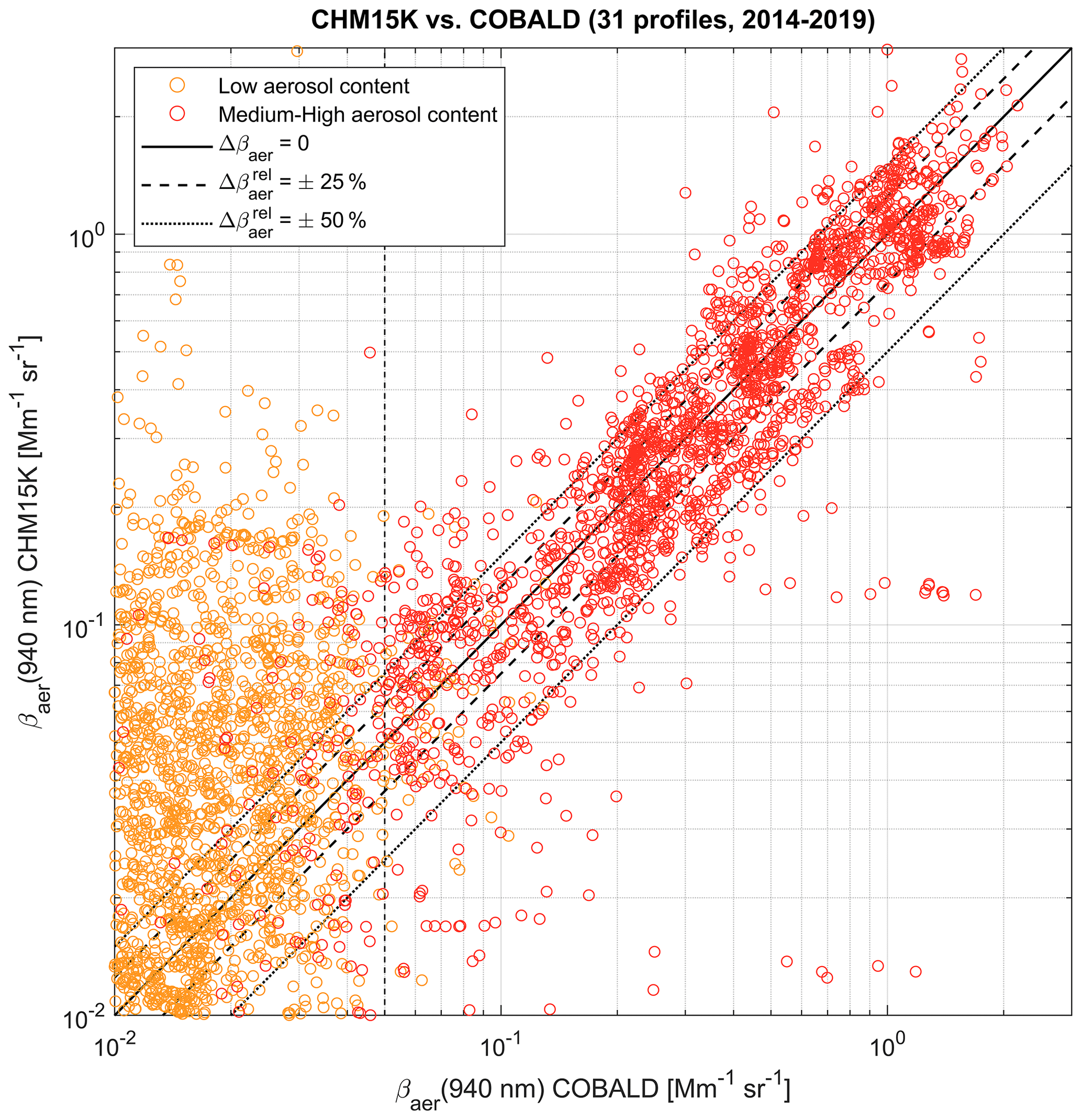
Figure 10 Statistical comparison of CHM15K vs. COBALD: scatterplot. All medium-high-aerosol-content (red circles) and low-aerosol-content (orange circles) data points of aerosol backscatter coefficient (β_aer) at 940 nm measured by CHM15K (y axis) vs. β_aer at 940 nm measured by COBALD (x axis). Thin black lines show 1:1 agreement (solid), ± 25 % difference (dashed) and ±50 % difference (dotted) isolines. The 0.05 Mm⁻¹ sr⁻¹ threshold in COBALD β_aer, separating low- from medium-high-aerosol-content data at 940 nm (as described in Sect. 3.3), is shown by a dashed vertical black line.

Figure 8 shows all data points of Δβ_aer at 940 nm for CHM15K−COBALD as a function of altitude, in both absolute backscatter coefficient units (panel a) and percent units relative to the COBALD signal (panel b). Analogously to Fig. 5, medium-high-aerosol-content data are shown as dark-red circles and low-aerosol-content data as orange circles. Note that the higher density of data points in Fig. 8 compared to Fig. 5 is due to the larger number of profiles considered for the CHM15K vs. COBALD comparison (31) relative to the RALMO vs. COBALD comparison (17) (see Sect. 2.3).

In absolute terms, medium-high-aerosol-content measurements by CHM15K are on average in good agreement with COBALD over the entire altitude range (Fig. 8a), yet their relative differences are characterized by a large statistical variability at all altitudes (Fig. 8b). The absolute differences in β_aer between CHM15K and COBALD are typically larger than observed for RALMO (Fig. 5a), despite β_aer being smaller at 940 nm than at 455 nm due to its spectral dependency. This highlights the lower signal-to-noise ratio of CHM15K compared to a high-power Raman lidar such as RALMO, which results in the large relative fluctuations in $\mathrm{\Delta }{\mathit{\beta }}_{\mathrm{aer}}^{\mathrm{rel}}$ in the free troposphere in Fig. 8b (especially for low-aerosol-content conditions).

Below 3 km altitude, the mean deviation profile of medium-high-aerosol-content measurements shows a slight overestimation of +5 % with respect to COBALD and a standard deviation of around 40 % (Fig. 8b). In this case, such a large spread of relative deviations can be also partly attributed (in addition to the effects mentioned in Sect. 4.2.1) to the uncertainty related to the assumption of a constant lidar ratio (50 sr) for all profiles made in the Klett inversion scheme for the retrieval of the CHM15K backscatter coefficient (see Sect. 2.1). This uncertainty is discussed in more detail in Sect. 4.3. For z > 3 km, the majority of medium-high-aerosol-content measurements (except one outlying profile, showing discrepancies of up to −0.5 Mm⁻¹ sr⁻¹ until 4 km altitude) stay within absolute deviations of ±0.2 Mm⁻¹ sr⁻¹ (Fig. 8a).

Figure 9 shows frequency-of-occurrence distributions of CHM15K−COBALD Δβ_aer at 940 nm for the altitude intervals of 0.8–3 km (panels a–b), 3–6 km (panels c–d) and 0.8–6 km (i.e., all altitudes: panels e–f), both for medium-high-aerosol-content data (red bars) and all data (black solid lines), calculated as in Fig. 6. The absolute (relative) δ ± σ for medium-high-aerosol-content data is +0.009 ± 0.185 Mm⁻¹ sr⁻¹ (+5 % ± 43 %) for 0.8–3 km altitudes, −0.081 ± 0.291 Mm⁻¹ sr⁻¹ (−43 % ± 72 %) for 3–6 km and −0.058 ± 0.205 Mm⁻¹ sr⁻¹ (−22 % ± 59 %) for all altitudes. As for RALMO, including low-aerosol-content data increases the frequency of occurrence of small absolute differences (Fig. 9a, c, e) yet reduces the frequency of occurrence of small relative differences (Fig. 9b, d, f). In particular for z > 3 km, we observe that the distributions of relative $\mathrm{\Delta }{\mathit{\beta }}_{\mathrm{aer}}^{\mathrm{rel}}$ for all data are significantly broader for CHM15K (Fig. 9d) than for RALMO (Fig. 6d). This is due to the low signal-to-noise ratio of CHM15K at high altitudes, together with the lower absolute β_aer signal at 940 nm compared to 455 nm.

Finally, Fig. 10 shows the scatterplot of all CHM15K vs. COBALD measurements of β_aer at 940 nm (between 0.01–3 Mm⁻¹ sr⁻¹). As in Fig. 8, medium-high-aerosol-content data points are shown as dark-red circles and low-aerosol-content data points as orange circles. The 0.05 Mm⁻¹ sr⁻¹ threshold in COBALD β_aer, separating low- from medium-high-aerosol-content data at 940 nm (as described in Sect. 3.3), is shown by a thin dashed black line. CHM15K and COBALD show a generally good correlation in the medium-high-aerosol-content range, although discrepancies exceeding ±50 % are often observed, and a very large spread of deviations for low-aerosol-content data (Fig. 10). The Pearson correlation coefficient is $\mathit{\rho }=+\mathrm{0.72}$ for altitudes 0.8–3 km a.s.l., +0.24 for altitudes 3–6 km a.s.l. and +0.62 for all altitudes, indicating a generally high degree of correlation at low altitudes (yet with smaller ρ than for RALMO) and a lower correlation at high altitudes. We observe that in the range of most frequently observed β_aer in the PBL (approximately 0.2–1 Mm⁻¹ sr⁻¹), CHM15K regularly exceeds deviations of ± 25 % with respect to COBALD (Fig. 10), while for RALMO in the corresponding range of β_aer (0.4–2 Mm⁻¹ sr⁻¹ at 455 nm), the fraction of individual differences exceeding ± 25 % is significantly smaller (Fig. 7). This highlights a generally better precision of RALMO with respect to CHM15K, even at medium-high-aerosol-content conditions.

4.3 Discussion

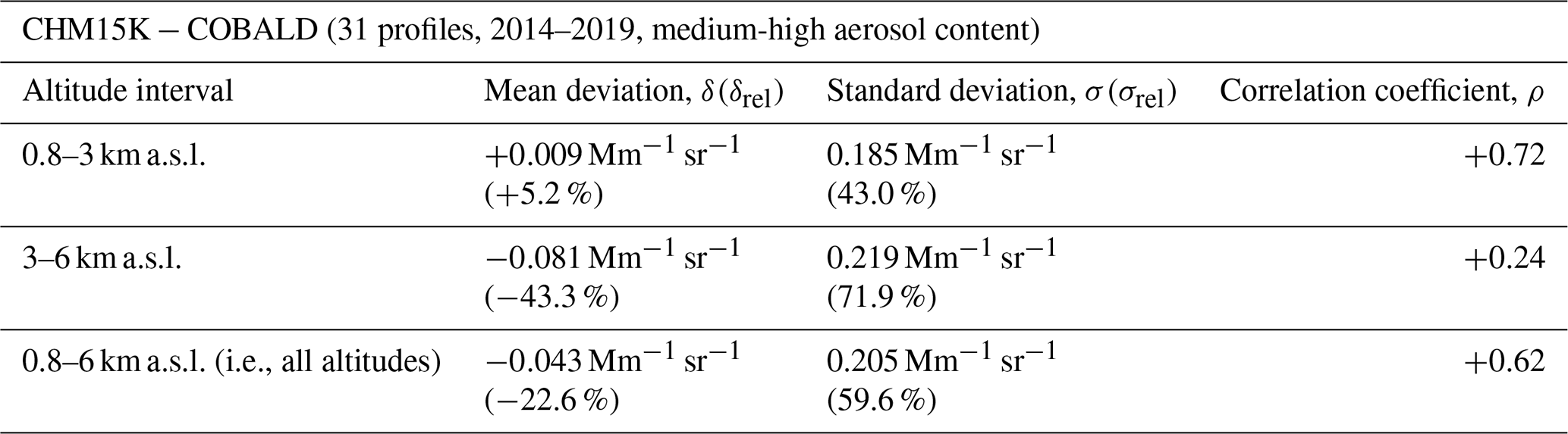
The results of the statistical comparison for medium-high-aerosol-content data are summarized in Tables 2–3. In general, both RALMO and CHM15K achieve a good agreement with COBALD in terms of mean deviations in the PBL (${\mathit{\delta }}_{\mathrm{rel}}=-$2 % for RALMO and +5 % for CHM15K for z < 3 km), while simultaneously they show relatively large standard deviations, even at low altitudes (σ_rel= 37 % for RALMO and 43 % for CHM15K for z < 3 km). As mentioned throughout the paper, this can be at least partly attributed to a number of methodological and technical aspects of our comparison, namely the uncertainties associated with the wavelength conversion and the FOV correction as well as spatial- and temporal-variability effects.

Table 3 Statistical comparison of CHM15K vs. COBALD: results for medium-high aerosol content. For each altitude interval, we show mean deviation (in both absolute units, δ, and percent units relative to COBALD, δ_rel) and standard deviation (in both absolute units, σ, and percent units relative to COBALD, σ_rel) at 940 nm as well as Pearson correlation coefficient (ρ).

The first uncertainty is related to the assumption of the COBALD-derived AE profiles to perform the wavelength conversion of the lidar data. From Eq. 2 we can derive that an error of 0.2 in AE, which is a conservative estimate considering the small difference between the wavelengths that are compared, results in an error of 5 % in β_aer for the 355–455 nm conversion and 2.5 % for the 1064–940 nm conversion. The second factor is related to the empirical implementation of the FOV correction, which involves several assumptions and simplifications (see Sect. 3.3). From Fig. 2b, we can estimate an uncertainty of up to ±20 % in β_aer for the PBL (for both 455 and 940 nm) due to variability in the correction factors in the range of AE = 0.8–1.5, which is not resolved by the parameterization of the FOV correction factors in the AE space (Fig. 2d). Finally, the balloon's horizontal drift with altitude away from the lidar beam and the different integration times of the two techniques can also affect the spread of their measurements. These effects can lead to large discrepancies over small altitude layers, as in the case of strong vertical gradients in β_aer (e.g., top of boundary layer; Fig. 4a–d), as well as potentially over larger altitude regions due to the horizontal gradient of the β_aer field around the station (e.g., in the case of the strongly outlying profiles of the statistical comparison; see Figs. 5, 8). The lack of information on the aerosol size distribution and the high spatial and temporal variability in atmospheric aerosols prevent an accurate quantification of these artifacts, which inevitably affects the standard deviations of our statistical comparison.

In addition to these effects, the large spread of relative deviations below 3 km in the case of CHM15K−COBALD can also be related to the assumption of a constant lidar ratio (50 sr) for all profiles made in the Klett retrieval algorithm (see Sect. 2.1). Using a similar ceilometer (Jenoptik CHM15kx), Wiegner and Geiss (2012) estimate that an error of ±10 sr in lidar ratio leads to an error in β_aer smaller than 2 % in the boundary layer. Ackermann (1998) shows that 50 ± 10 sr represents well the expected range of variability in the lidar ratio of continental aerosol in the infrared spectrum for all RH conditions between 0 %–90 %. Therefore, this uncertainty conceivably plays a minor role compared to the effects discussed above.

Despite these limitations, the comparison of individual profiles (Sect. 4.1) shows that both RALMO and CHM15K are able to achieve an excellent agreement with COBALD measurements, including the correct representation of fine and complex structures in the β_aer vertical profiles (Figs. 3–4, S2–S3). In particular, the case study of 12 July 2018 (Fig. 4a-d) shows differences between the lidars and COBALD which are smaller than the expected statistical uncertainty associated with the remote-sensing measurements alone (10 %–15 %; see Sect. 2.1). This suggests that, under optimal conditions (such as no wind shear, uniform β_aer field, mono-modal aerosol size distribution), the deviations between the two lidars and COBALD are typically smaller than the average σ of our statistical comparison. Considering also the good linear correlation achieved by both lidars ($\mathit{\rho }=+$0.81 for RALMO and +0.72 for CHM15K for z < 3 km), we conclude that β_aer measurements by RALMO and CHM15K are in overall good agreement with in situ measurements by COBALD sondes up to 6 km altitude.

5 Conclusions

We have presented the first comparison of lower-tropospheric-aerosol backscatter coefficient (β_aer) profiles retrieved by remote-sensing instruments against independent in situ measurements. The two analyzed lidar systems, one research Raman lidar (RALMO) and one commercial ceilometer (CHM15K), were validated using simultaneous and co-located balloon soundings carrying a Compact Backscatter Aerosol Detector (COBALD), performed during the years 2014–2019 at the MeteoSwiss observatory of Payerne, Switzerland. COBALD provides high-precision in situ measurements of β_aer at two wavelengths (455 and 940 nm) and is used as the reference instrument. The β_aer profiles retrieved from RALMO (355 nm) and CHM15K (1064 nm) are converted to 455 nm and 940 nm, respectively, using the altitude-dependent Ångström exponent (AE) profiles retrieved from COBALD data. To account for the different receiver field-of-view (FOV) angles between the remote-sensing instruments (0.01–0.02^∘) and COBALD (6^∘), we derived a FOV correction using Mie-theory scattering simulations. The correction factors are parametrized as functions of AE to account for the size dependency of the solutions. For the statistical comparison, low- and medium-high-aerosol-content measurements are separated according to an empirical threshold in β_aer.

The comparison of individual profiles shows that both RALMO and CHM15K achieve a good agreement with COBALD β_aer measurements in the boundary layer and free troposphere up to 6 km altitude, including fine structures in the aerosol's vertical distribution. The mean ± standard deviation of RALMO−COBALD Δβ_aer (at 455 nm) for medium-high-aerosol-content data is −0.018 ± 0.237 Mm⁻¹ sr⁻¹ (−2 % ± 37 %) for altitudes 0.8–3 km a.s.l. and +0.001 ± 0.141 Mm⁻¹ sr⁻¹ (+6 % ± 38 %) for all altitudes between 0.8–6 km a.s.l. For CHM15K−COBALD, the mean ± standard deviation of Δβ_aer (at 940 nm) for medium-high aerosol measurements is +0.009 ± 0.185 Mm⁻¹ sr⁻¹ (+5 % ± 43 %) for altitudes 0.8–3 km and −0.058 ± 0.205 Mm⁻¹ sr⁻¹ (−22 % ± 59 %) for all altitudes. The Pearson correlation coefficient for medium-high aerosol content below 3 km altitude is +0.81 for RALMO vs. COBALD and +0.72 for CHM15K vs. COBALD, indicating a high degree of linear correlation between both lidars and the in situ measurements. For altitudes above 3 km (i.e., in the free troposphere), absolute deviations generally decrease, while relative deviations increase due to the prevalence of low-aerosol-content air masses. The standard deviations of medium-high-aerosol-content data between 3–6 km altitude are 38 % (0.068 Mm⁻¹ sr⁻¹) for RALMO−COBALD and 59 % (0.205 Mm⁻¹ sr⁻¹) for CHM15K−COBALD, which denotes the lower signal-to-noise ratio of CHM15K compared to a high-power Raman lidar system such as RALMO.

While both RALMO and CHM15K agree well with COBALD in terms of mean deviations, the statistical comparison is characterized by relatively large standard deviations for both instruments at all altitudes. As discussed in Sect. 4.3, this can be at least partly attributed to a number of technical aspects of our comparison, most notably the uncertainty associated with the FOV correction and spatial- and temporal-variability effects (related to the balloon's horizontal drift with altitude and different integration times), which contribute to the spread of the measurements. Due to the lack of information on the aerosol size distribution and the high spatial and temporal variability in atmospheric aerosols, these effects cannot be accurately quantified. Nevertheless, the excellent agreement observed in individual profiles, including fine and complex structures in the aerosol's vertical distribution, shows that under optimal conditions (no wind shear, uniform β_aer field, mono-modal aerosol size distribution), the deviations between the two lidars and COBALD are typically comparable to the estimated statistical errors in the remote-sensing measurements alone (10 %–15 %). Similar or even larger discrepancies are also reported in the literature between single-wavelength elastic-backscatter and Raman lidars (e.g., Matthais et al., 2004; Tsaknakis et al., 2011; Madonna et al., 2018) as well as between different Raman lidar algorithms (Pappalardo et al., 2004).

Considering the many uncertainties that characterize the retrieval of aerosol backscatter profiles from lidar instruments, from technical and instrumental effects to issues related to the mathematical treatment of the data (e.g., Pappalardo et al., 2004), our validation using fully independent in situ measurements is particularly valuable. Despite the limitations outlined above, results demonstrate that both single-wavelength (ceilometer) and Raman lidars can provide altitude-resolved measurements that are quantitatively consistent with high-precision balloon-borne measurements over the PBL and free-troposphere altitude regions. Overall, we conclude that aerosol backscatter coefficient measurements by the RALMO and CHM15K lidar systems are in satisfactory agreement with in situ measurements by COBALD sondes up to 6 km altitude.