the Creative Commons Attribution 4.0 License.
the Creative Commons Attribution 4.0 License.
 | 15 Feb 2021
Quasi-coincident observations of polar stratospheric clouds by ground-based lidar and CALIOP at Concordia (Dome C, Antarctica) from 2014 to 2018
Francesco Colao
Francesco Cairo
Ilir Shuli
Andrea Scoccione
Mauro De Muro
Michael Pitts
Lamont Poole
Luca Di Liberto
Polar stratospheric clouds (PSCs) have been observed from 2014 to 2018 from the lidar observatory at the Antarctic Concordia station (Dome C), included as a primary station in the NDACC (Network for Detection of Atmospheric Climate Change). Many of these measurements have been performed in coincidence with overpasses of the satellite-borne CALIOP (Cloud Aerosol Lidar with Orthogonal Polarization) lidar, in order to perform a comparison in terms of PSC detection and composition classification. Good agreement has been obtained, despite intrinsic differences in observation geometry and data sampling. This study reports, to our knowledge, the most extensive comparison of PSC observations by ground-based and satellite-borne lidars.
The PSCs observed by the ground-based lidar and CALIOP form a complementary and congruent dataset and allow us to study the seasonal and interannual variations in PSC occurrences at Dome C. Moreover, a strong correlation with the formation temperature of NAT (nitric acid trihydrate), TNAT, calculated from local temperature, pressure, and H2O and HNO3 concentrations is shown. PSCs appear at Dome C at the beginning of June up to 26 km and start to disappear in the second half of August, when the local temperatures start to rise above TNAT. Rare PSC observations in September coincide with colder air masses below 18 km.
- Article
(3944 KB) - Full-text XML
- BibTeX
- EndNote


Long-term ground-based and satellite-borne lidar observations provide valuable climatological data and allow monitoring of the state of the polar stratosphere and comparison with chemistry climate models (CCMs). Several Antarctic stations have been equipped with lidar for PSC observations since the 1980s. The longest time records are from Dumont D'Urville (1989–1998, 2006–present) (Santacesaria et al., 2001; David et al., 1998, 2010) and McMurdo (1990–2010) (Adriani et al., 1992, 1995, 2004; Di Liberto et al., 2014; Snels et al., 2019). The McMurdo stratospheric lidar was transferred to Concordia station at Dome C and has been operational since 2014. Concordia station has the advantage of being on the Antarctic plateau, far from the coast and well within the polar vortex during most of the winter (see Fig. 1). Meteorological conditions are in general more stable than those at the lidar stations located on the coast (McMurdo, Dumont D'Urville, Davis, Syowa, Rothera, Belgrano II), and tropospheric clouds rarely obstruct the PSC observations. South Pole station is also located far from the coast and as such shares the advantages of Dome C, but unfortunately all three lidar systems that have been operated there (Fiocco et al., 1992; Fua et al., 1992; Simpson et al., 2005; Huang et al., 2007; Campbell and Sassen, 2008) were without a depolarization channel, and thus they are limited in classifying the composition of the observed PSCs.
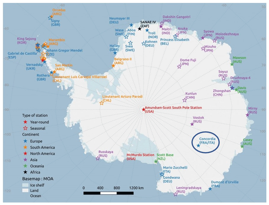
Figure 1The map shows the main research stations in Antarctica.
The CALIPSO (Cloud-Aerosol Lidar and Infrared Pathfinder Satellite Observations) satellite was launched in April 2006 as a component of the A-Train satellite constellation (Stephens et al., 2002, 2018). With an orbit inclination of 98.2∘, it provides extensive daily measurement coverage over the polar regions of both hemispheres, up to 82∘ in latitude. The primary instrument of CALIPSO is the Cloud Aerosol Lidar with Orthogonal Polarization (CALIOP). CALIOP has extensively been used for observing PSCs (Pitts et al., 2009, 2011, 2013, 2018).
The goal of this study is twofold. The first objective is to develop a methodology to obtain a consistent set of PSC data obtained from ground-based and CALIOP observations, while reducing possible biases. The second is to demonstrate how this complementary set of data can be used to study seasonal and interannual variations in PSC occurrences at Dome C.
Ground-based and satellite-borne lidars are complementary and can provide useful data for climate studies. It would be desirable if the ground-based data would be representative for a certain area around its location and could be used to fill gaps in time between CALIOP overpasses. However, important biases may occur when comparing PSC detection and classification of ground-based lidars and CALIOP. These can be summarized as follows.
-
Different observation geometry. The air masses observed by ground-based lidar and CALIOP are different in size and shape. Since the ground-based lidar observes from below the clouds and the satellite-borne lidars from above at a much larger distance, the signal-to-noise ratio () has a different dependence on altitude. For the ground-based lidars the decreases with altitude, while the for CALIOP has only a small dependence on altitude (between 12 and 30 km). The quality of the data obtained by ground-based lidars depends on the tropospheric cloud cover (see e.g., Tesche et al., 2021).
-
Different detection and classification thresholds. Achtert and Tesche (2014) showed how the different schemes for detection and classification of PSCs cause large biases, by applying a variety of schemes using different thresholds to the same dataset. Generally ground-based lidars use fixed thresholds, while the v2 algorithm developed by the CALIOP team uses dynamical thresholds.
-
Different duration for the acquisition of a vertical profile. Ground-based lidars usually integrate over 30–60 min, CALIOP takes “snapshots” with a duration of several seconds. This implies that ground-based observations integrate the optical parameters over a lapse of time while air masses of different composition might pass over the lidar station and thus are apt to observe PSC types with average values of the optical parameters at the cost of underestimating others. This will be addressed in more detail when discussing the differences in ground-based and CALIOP composition classification.
-
The probability that the ground-based lidar and CALIOP observe the same air mass or part of the same homogeneous PSC cloud depends on the horizontal extension of these clouds.
Here we will address the impact of each of these factors. We tried to reduce the effect of different detection and classification thresholds by applying exactly the same detection and classification algorithm and by also using dynamical thresholds for the ground-based data, taking into account the dependence on altitude of the ground-based data. We also mitigate the differences caused by observing different air masses by comparing quasi-coincident data. The potential success of comparing quasi-coincident observations will be evaluated by using the CALIOP overpasses in a limited area around Concordia station (about 200 km × 200 km) to estimate the horizontal extension and homogeneity in terms of PSC composition. We then discuss the impact of the different observation geometries as well as the effects of different durations of the measurements.
In a previous paper (Snels et al., 2019) the full dataset of PSC observations by ground-based and satellite-borne lidar above McMurdo has been statistically compared in terms of detection and composition classification of PSCs. In the McMurdo study all ground-based lidar and CALIOP data within a longitude–latitude box (7∘ × 1∘) centered on McMurdo, without further constraints, were taken into account. This implies that ground-based data recorded on days without CALIOP overpasses in the longitude–latitude box were included in the statistical analysis, as well as all CALIOP profiles within the box. Also, the detection and classification thresholds and were fixed values or averages over longer periods. The number of quasi-coincident observations was not sufficient to perform an analysis similar to the one presented here, but a statistical analysis of the PSC occurrences over periods of 4 months (in some cases 1 month) showed an overall agreement.
The measurements at Dome C were synchronized from the start with the near overpasses of CALIOP, and thus a large number of data were available to study quasi-coincident observations, by comparing the ground-based observations with single CALIOP profiles acquired at the closest possible distance from the ground station and within 30 min of the ground-based observation. For the CALIPSO PSC product, a single vertical profile consists of an average over a 5 km long segment of the flight track. The quasi-coincident approach has not been applied to the McMurdo data since too few quasi-coincidences were available.
If we want to use ground-based and CALIOP data together, in a complementary and congruent way, we need to verify whether both lidars observe essentially the same scene, in terms of PSC detection and composition. Much depends on the spatial extent of the PSC fields and their homogeneity in terms of particle composition. If the PSC's spatial extent is generally small with respect to the average closest distances of the footprint of the satellite-borne lidar with respect to the ground station, our approach is condemned to fail. If, however, PSC fields extend over many tens or hundreds of kilometers, our approach may yield valuable results. The position of Dome C on the central plateau, with no important orographic features present, implies that the temperature fields should be mainly of a synoptic nature, with few local perturbations. This would cause the PSCs to have a large extension and a predominantly homogeneous composition. We will show by studying PSCs observed during CALIOP overpasses close to Dome C that in most cases the PSC fields have sufficiently large extension to allow for a comparison of almost coincident observations. Of course this is valid for the detection, while a comparison of the composition would require that the PSCs also be of a homogeneous composition over these scales. We will also address this problem and show that in many cases the PSC composition is substantially homogenous; i.e., more than two-thirds of the CALIOP overpasses in the box around Dome C at a specific vertical level have at least 75 % of PSCs of the same composition. It should be stressed that the results presented here are restricted to the area around Dome C and might be very different for other locations in Antarctica.
The formation of PSCs depends on the availability of condensation nuclei, temperature, and number densities of water and nitric acid. Nitric acid trihydrate (NAT) particles are in thermodynamic equilibrium with the gas phase at about 6 K above the ice frost point (Hanson and Mauersberger, 1988), while liquid PSCs in the form of supercooled ternary solutions (STSs) may form below temperatures of about 3 K above the ice frost point. Finally ice PSCs form below the ice frost point. While ice evaporates once the temperature exceeds the ice frost point, NAT and STSs may survive for some hours/days above their equilibrium temperature. Here, we compare the occurrence of PSCs, as detected by the ground-based lidar and CALIOP, with the formation temperature of NAT. All species discussed here, NAT, STSs, ice and their mixtures, form below TNAT, and one would expect to observe PSCs when the local temperature is below TNAT, although NAT and STSs might also survive for some time above this temperature. We observe how PSC occurrences drop rapidly in the third and fourth weeks of August, when the local temperatures exceed TNAT. Seasonal and interannual variations in PSC occurrences are seen to be dependent on the position of the cold polar vortex. Here we use TNAT as a delimiter of the area where PSCs may be formed.
A lidar has been operated at the Antarctic station Concordia at Dome C since 2014, as a continuation of the long-term observations at McMurdo (1991–2010), with the goal of measuring the atmospheric backscatter with parallel and perpendicular polarization with respect to the emitted laser radiation. The lidar observatory uses most of the hardware previously used at McMurdo, with small improvements. In addition, the instrument has been adapted to the harsher environment at Dome C. In particular a triple glass view port has been mounted above the telescope in order to have a better insulation from the outside temperature. Recently, the observatory has been equipped with a remote control of the laser and the data acquisition system, allowing for a complete control of the measurements from the main buildings at Dome C, at a distance of about 400 m from the observatory, or from our home institute in Italy.
Dome C is well within the stratospheric polar vortex from mid-June to the end of September (see e.g., Waugh and Randel, 1999), although climatologically the coldest part of the vortex migrates towards the Antarctic Peninsula starting in the second half of August. Recently Dome C was identified as one of the most favorable locations for the observation of PSCs (Tesche et al., 2021). In general the weather conditions are rather stable with respect to McMurdo and other coastal lidar stations, and the lidar has been operated satisfactorily from 2014 on, during the Antarctic winter, with the exception of 2019, when severe instrumental problems occurred. The lidar is operated by winter-over scientists of the PNRA (Piano Nazionale della Ricerca in Antartide) during the Antarctic winter, typically from the end of May until the end of September to cover the whole period of PSC occurrence. The lidar is operated once or twice per day, when meteorological conditions are favorable. If possible, the observations are synchronized with overpasses of the CALIPSO satellite, when its footprint is within 100 km from Concordia station. Single vertical profiles with a vertical resolution of 60 m have been recorded by averaging 30 min of acquisition. All lidar data have been deposited into the NDACC database (Snels, 2019), where they are available to the scientific community.
CALIOP is a two-wavelength lidar, measuring backscatter at wavelengths of 1064 and 532 nm, with the latter signal separated into parallel and cross polarization, with respect to the polarization of the outgoing laser beam. Details on CALIOP can be found in Hunt et al. (2009) and Winker et al. (2009). The orbital period of CALIPSO is about 98 min, which results in about 14–15 orbits per day. This results in two overpasses per day at distances ranging from 0 to 400 km from the ground-based lidar at Dome C, one on an ascending and the other on a descending orbit. Here we consider all overpasses within a longitude–latitude box (7∘ × 2∘) centered on Concordia station, resulting in about 20 overpasses per month. The 7∘ × 2∘ box corresponds roughly to a square of 200 km × 200 km. The speed of the CALIOP footprint on the surface is about 400 km/min which implies that an overpass in the box lasts on average about 30 s. The orbit track of CALIOP in the box has a swath width of about 100 m and consists of a number of vertical profiles averaged over 5 km along the flight track.
The different sampling times and observation geometries of the ground-based lidar and CALIOP imply that it is extremely difficult to obtain “real” coincidences. An interesting approach has been suggested by David et al. (2012) and Achtert et al. (2011), who used trajectories calculated from wind velocities and directions to connect the air masses observed by ground-based lidar and CALIOP. Of course this method is limited to very few intersections and depends strongly on the altitude, since the wind velocity increases with altitude. The average wind speed ranges from about 50 to 110 km/h between 10 and 20 km of altitude, but maximum wind speeds exceed 200 km/h. The wind direction at Dome C is mostly between NE and SE. We have explored the possibility of applying the trajectory approach to our data, but the number of coincidences is very low and not homogeneously distributed for all altitudes, and this method has thus been discarded. Instead we compared ground-based data with the closest profile on each CALIPSO flight track (within 100 km) and with an overpass time within 30 min of the ground-based observation. This is a good compromise for obtaining a significant number of comparisons and having a reasonable probability that both lidars observe similar air masses, although not perfectly coincident. The comparison is made considering the detection and composition classification of PSC clouds.
2.1 PSC detection and classification criteria for the CALIPSO v2 data
The CALIOP v2 PSC detection and composition classification algorithm has been used to create the recently released CALIOP v2 PSC mask database covering the period from June 2006 to October 2019. Here we compare these v2 data with ground-based observations at Dome C from 2014 to 2018. Major enhancements in the v2 algorithm over earlier versions include daily adjustment of composition boundaries to account for effects of denitrification and dehydration and estimates of the random uncertainties u(β⟂) and u(R) due to shot noise in each data sample, which are used to establish dynamic detection thresholds and composition boundaries. The CALIOP v2 algorithm is represented pictorially in Fig. 2 and is described in more detail in Pitts et al. (2018) and Snels et al. (2019).
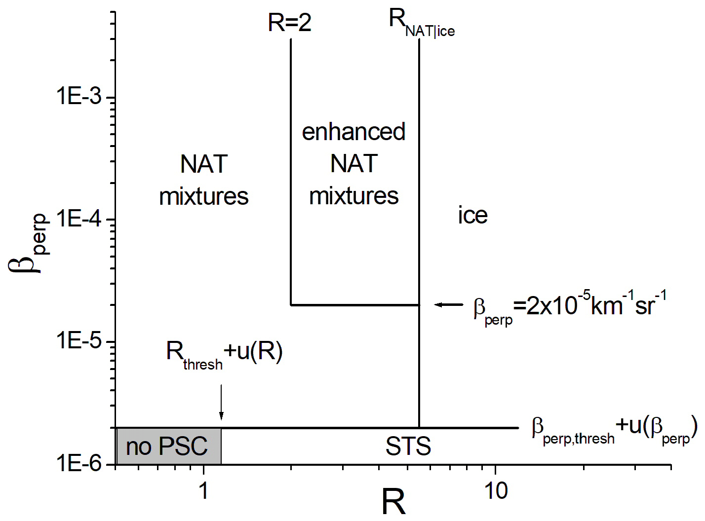
Figure 2The figure shows the detection and classification criteria of the V2 CALIOP algorithm. The classification as STSs, NAT mixtures, enhanced NAT mixtures and ice requires that threshold conditions for R and/or β⟂ are satisfied. Please note that the thresholds are dynamic thresholds, except for the threshold on R that separates NAT mixtures from enhanced NAT mixtures. The figure has been adapted from Snels et al. (2019).
2.2 PSC detection and composition classification criteria for the ground-based lidar data
In order to compare the ground-based lidar data to the CALIOP data, we have adopted a similar algorithm which follows the same approach and uses the same optical parameters as the v2 CALIOP algorithm (see Fig. 2). The v2 background aerosol thresholds and Rthresh have been calculated in a different way, to take into account a series of errors due the small deviations from the calculated molecular scattering profiles in clear-sky conditions (i.e., absence of aerosols). Then statistical errors caused by the photon-counting process and thus depending on the altitude and on the possible attenuation in the lower troposphere have been taken into account to calculate u(β⟂) and u(R) and create the dynamic thresholds for detection and classification.
2.2.1 Data processing
Raw data consist of photon counts recorded in 400 ns bins, corresponding with a vertical resolution of 60 m, and are accumulated in records with a duration of 2 min. First the data are averaged and the background count is determined from the first 40 bins, before the laser fires. The background is then subtracted from the signals. The lidar records two channels, one collecting the signal with the polarization parallel to the laser emission and the other with perpendicular polarization. The two components are separated by using two polarizing beam-splitter cubes. The perpendicular polarization is in theory due to the depolarization by molecules and aerosols. In practice some instrumental factors may contribute to the perpendicular polarization, such as a small perpendicular component of the laser emission, the residual transmission/reflection of the unwanted component of the polarizing beam-splitter cubes and other effects. In our case there is a substantial contribution due to the triple viewport. Starting from the lidar equation
we can express the signals on the two detectors, if we neglect the extinction, while only considering the crosstalk as originating from the optical elements (polarizer and viewport), as
where g1 and g2 are the gain factors of the two detectors, and CT is the crosstalk from the parallel channel to the perpendicular channel. We neglect the crosstalk from the perpendicular to parallel channels.
In order to facilitate the interpretation of the signals and the detection of clouds, we divide both signals by the molecular backscatter coefficient and multiply by z2 and we get
The molecular backscatter coefficient has been calculated by using local temperature and pressure provided by radiosoundings and, where these were not available, from the NCEP (National Centers for Environmental Prediction).
We can normalize these expressions to 1, where no aerosols are present (typically between 26 and 30 km). The normalized expressions become
where
With some algebra we can now obtain expressions for R and β⟂:
and
where . In our case, using an optical bandpass filter centered at the laser wavelength (532 nm) with a full width at half maximum (FWHM) of 2 nm, δmol is 0.007 (Behrendt and Nakamura, 2002).
Now we can see that the crosstalk CT can be written as
The two parameters rn∥ and rn⟂ can be determined from the calibration process for aerosol-free regions, so we only need the ratio of the two gain constants of the two detection channels, which can be determined by switching the detectors, or by more sophisticated methods (Snels et al., 2009).
Now we perform the correction for extinction, using the Klett retrieval scheme (Klett, 1981) and the proportionality between β and the extinction coefficient as reported by Gobbi (1995), and we use the ratios obtained after the correction to calculate R(z) and β⟂(z).
2.2.2 Error processing
The statistical errors derived from the photon-counting process, u(β⟂) and u(R), have been determined from the raw signals and are thus dependent on z. The background aerosol thresholds and Rthresh have been determined mainly by comparing with clear-sky profiles and have been expressed in terms of the ratios and . They are estimated to be 1.05 for and for . For z<16 km, these values increase gradually to 1.2 in order to take into account an insufficient correction of saturation effects.
2.2.3 PSC detection and composition classification
PSC detection and classification from lidar measurements with orthogonal polarization are based on two optical parameters derived from the optical signals with parallel and perpendicular polarization with respect to the laser. Here we use a method that approximately follows the v2 classification and detection scheme (see also Snels et al., 2019), proposed by Pitts et al. (2018) for the classification of the CALIOP PSC data and using the backscatter ratio R and the perpendicular backscatter coefficient β⟂.
The backscatter ratio R and the perpendicular backscatter coefficient β⟂ have been determined from the raw data as described above. The optical parameters obtained in this way, as well as their errors, were smoothed to the vertical scale of the CALIOP profiles, with a vertical resolution of 180 m per layer or pixel as we will call the single bins on a profile from now on. The detection thresholds for the backscatter ratio R were thus determined to be Rthresh+u(R), and the threshold for β⟂ is . This results in dynamic thresholds that vary from profile to profile, for instance due to attenuation of the lidar signal by cirrus clouds, and vary with altitude, mostly because of the statistical errors in the photon-counting process.
In order to detect a PSC, it is sufficient that either the backscatter ratio R or the perpendicular backscatter coefficient β⟂ exceeds the respective threshold. A final step of the processing requires that at least five consecutive points on a vertical profile are identified as PSCs, in order to avoid the appearance of “spikes” in the profiles. Sequences of fewer than five PSC points are thus considered to be non-PSCs. This procedure is similar to the coherence criterion used for the CALIOP data.
2.2.4 PSC composition
Composition classification for ground-based PSCs is nearly identical to the CALIOP v2 procedure, the exception being that we use values of RNAT|ice reported for the closest profiles in the v2 CALIOP data files. The borderline value to discriminate between STS and NAT is equal to the detection threshold for β⟂, exactly the same as for the CALIOP data.
The maximum number of overpasses within a distance of 100 km is about 20 per month, resulting in about 80 possible coincidences per PSC season, considering the observation period from June until September. However, we must consider several practical issues: sometimes the ground-based lidar cannot be operated due to adverse weather conditions, and after the end of the austral winter, the day illumination might affect the lidar measurements, reducing the maximum altitude with an acceptable signal-to-noise ratio. Also, the CALIOP instrument is subject to periods of inactivity, although very rarely.
Table 1The number of available data and the detection statistics of both lidars have been listed. The column “detected” indicates when both ground-based lidar and CALIOP detect a PSC or they do not detect a PSC in the same vertical bin. The other two columns indicate all cases when only one of the instruments detects a PSC in a specific vertical bin. Only bins below 26 km have been considered, since very few PSCs have been observed above 26 km.
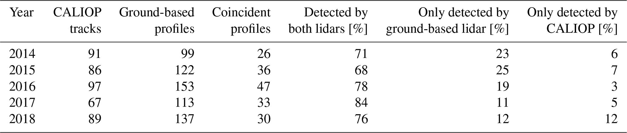
Table 1 shows some statistics illustrating the number of data acquired and actually used for comparison. Note that Table 1 includes all CALIOP tracks passing within a 200 km × 200 km square around Dome C, also including some tracks with a closest distance of more than 100 km. This explains why the number of CALIOP overpasses might be slightly larger than the 80 overpasses mentioned before. Throughout this paper, the comparison for detection and composition classification will be performed by comparing vertical bins, with the same height and a thickness of 180 m, one of the ground-based lidar profiles and the other of the nearest CALIOP profile. From now on we will refer to these bins as pixels, since each bin will be color coded in the figures in correspondence with the composition of the PSC. In our analysis we will consider only pixels between 12 and 26 km, since very few PSCs have been observed above 26 km, and inclusion of the pixels above 26 km would not be a good measure for comparison.
3.1 Statistical analysis of CALIPSO observations in the box around Dome C concerning PSC extension and homogeneity of composition
Since almost no exact coincidences are available, we compare the ground-based profiles acquired within 30 min from the CALIOP overpass with the closest point on the overpass. This results in an average distance between the closest points and the location of Dome C of about 50 km. The average time difference is about 15 min, corresponding with a distance of about 15–30 km, considering the average wind speed between 10 and 20 km of altitude. Thus we might say that there is a good probability that the quasi-coincident observations by the ground-based lidar and CALIOP observe the same PSC cloud as long as the PSC clouds around Dome C have a sufficiently large horizontal extension (approximately on the order of 50 km or more).
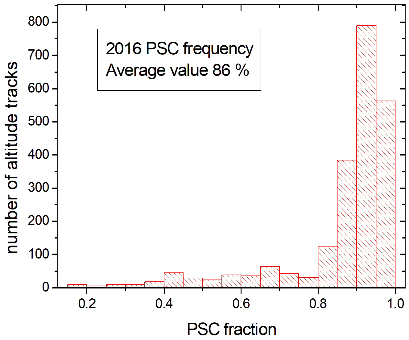
To get an idea of the horizontal extension of the PSC clouds and the homogeneity of these clouds in terms of the different PSC species, we examined all CALIOP overpasses passing within the 200 km × 200 km square around Dome C and with a minimum distance of less than 120 km, resulting in 369 tracks for the 5 years (2014–2018). The average length of each overpass track (i.e., the part of the overpass within the box) was about 180 km. We observed that 88 tracks did not contain PSCs at all. This means that for these tracks (23.8 % of the total) no PSC was detected in the CALIOP database for any of the vertical levels from 12 to 30 km. All the altitude levels for the remaining 281 tracks were then tested to evaluate the PSC horizontal extent for all vertical levels on a 180 m grid. The statistical analysis is performed by considering the sequence of pixels at the same height on the same overpass. (A pixel is a point on a vertical profile. Each pixel represents a volume of 180 m (height) × 100 m (horizontal swath of the CALIOP track) × 5000 m (distance between profiles on the overpass track). The number of pixels with a positive detection for PSC with respect to the total number of pixels on the overpass track in the box is a measure of the continuity of the cloud. For example, when we find that 30 pixels out of 36 pixels have a positive PSC detection flag, we have a fraction of 83 % PSC pixels on this track, which can be considered an almost continuous PSC cloud along the track. Thus the fraction (percentage) of segments with a positive PSC detection is calculated for each overpass track. When taking into account all 281 overpasses at all heights (equal to the number of overpasses multiplied by the number of vertical “levels” of 180 m height, from 12 to 26 km), we can obtain a statistical distribution that indicates how often an overpass track, between 12 and 26 km, has a certain PSC fraction. The results of this procedure are illustrated for 2016 in Fig. 3. Results are also similar for the other years. It can be observed that 83.5 % of the altitude tracks have more than 80 % of positive PSC detection. This implies that for 83.5 % of the overpasses PSC clouds have approximately a horizontal extension of at least 150 km.
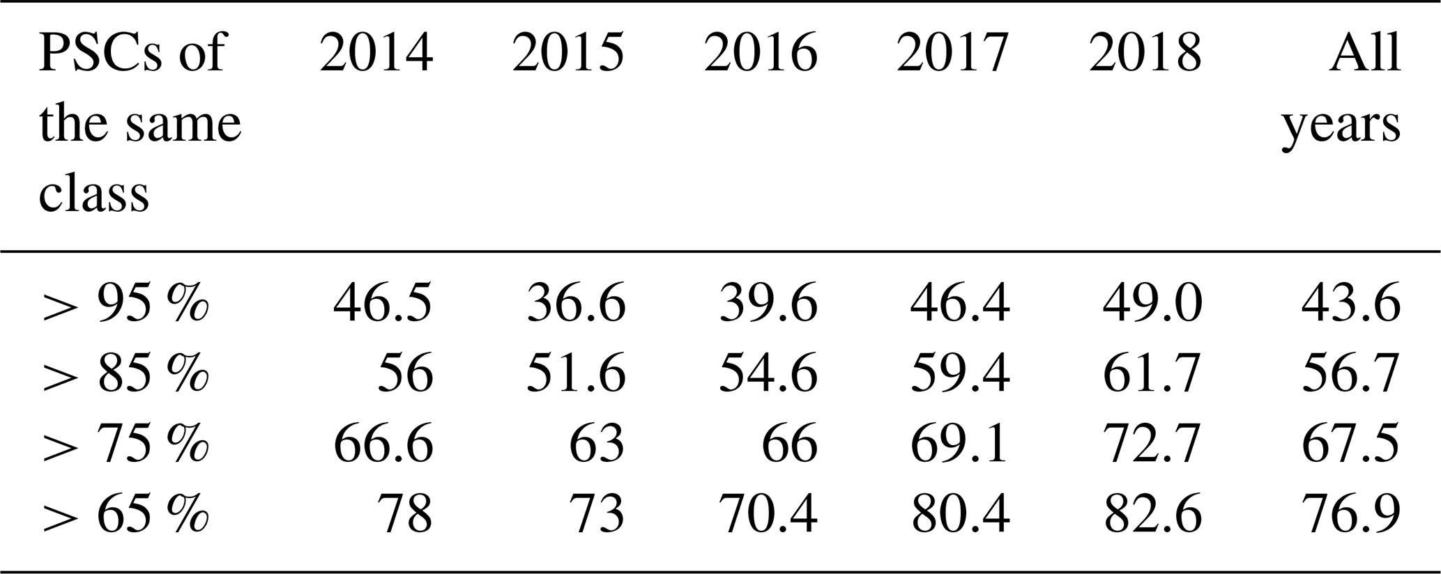
A second test has been performed to quantify how much the PSC composition varies along the track. The CALIOP data provide a detection flag and a composition classification for each segment, so we now consider the classification of each pixel, in order to get a measure for the homogeneity of the PSC clouds in terms of the PSC species. For this test we consider four PSC classes: STS, NAT mixtures, enhanced NAT mixtures and ice. We count the number of PSC segments along each orbit track at each altitude that belong to one of these four classes and obtain fractions for all four species. We consider the total number of horizontal slices of all overpasses (78 slices of 180 m, from 12 to 26 km, multiplied by the number of overpasses), and we count the number of slices where either STSs, NAT mixtures, enhanced NAT mixtures or ice represent more than 95 % of all segments with PSCs. Dividing this number by the total number of slices, we obtain the percentage of horizontal slices where one composition class is present for more than 95 %. The results are displayed in Table 2. Table 2 shows that a fair percentage of the detected PSC layers have an almost uniform PSC composition (on average 43.6 % of all layers), but evidently about 25 % of all PSC layers have at least one-third minor species, and in some cases there might be three PSC classes on the same layer (a layer is 180 m). In conclusion, as far as the CALIOP overpasses might be considered a valid representation of the PSC population in the box around Dome C, we might say that if PSCs are present in a layer, their horizontal extension is at least of the order of 100–150 km. On the other hand, although different PSC classes might exist in the same layer, the composition is homogeneous over a substantial portion of the layer. Of course these conclusions should be interpreted with some care since we do not have a two-dimensional PSC field at disposition, and we base our conclusions only on one-dimensional tracks. However, the overpasses have different directions, due to the ascending and descending orbits of CALIPSO, and thus many overpasses will ultimately fill a two-dimensional field.
Table 2The percentage of pixels on the altitude tracks with at least X percent of PSCs of the same class.
3.2 Comparison of ground-based and CALIOP data for 2015–2018
Now that we have some confidence that a comparison between ground-based and CALIOP data at an average distance of 50 km and within 30 min of the observation is a reasonable way of proceeding, we will illustrate the full procedure of detection and composition classification comparison.
The detection and composition classification of the PSCs in the CALIOP data are based directly on the CALIOP v2 PSC Mask database, while for the ground-based data we have applied the detection and classification scheme as has been discussed above. Table 1 shows how the data reduction proceeds: from a large number of CALIOP and ground-based vertical profiles only about 25 %–30 % remain as we consider only coincident profiles.
Figures 4, 5, 6 and 7 (left columns) show all measured profiles for the years 2015–2018 (excluding 2014, being a year with fewer data and starting only after 13 July) that meet the coincidence criteria (closest CALIOP profile within 30 min of ground-based observation time). Please note that on several days no PSCs at all were detected in the coincident profiles. Although these clear-sky profiles are a minority of the measurements, the two datasets also agree rather well for these clear-sky profiles, and thus they have been included in the detection statistics (see Table 1).
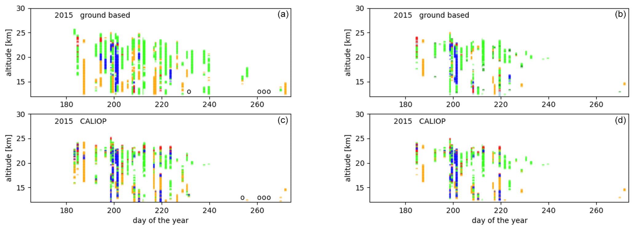
Figure 4All quasi-coincident observations (a, c) and only those where PSCs were observed by both lidars (b, d) for 2015 above Dome C. (a, b) Ground-based lidar. (c, d) CALIOP above Dome C. The different colors indicate PSCs of different composition. Green: NAT mixtures; yellow: STS; red: enhanced NAT mixtures; blue: ice. The circles indicate measured profiles without PSCs.
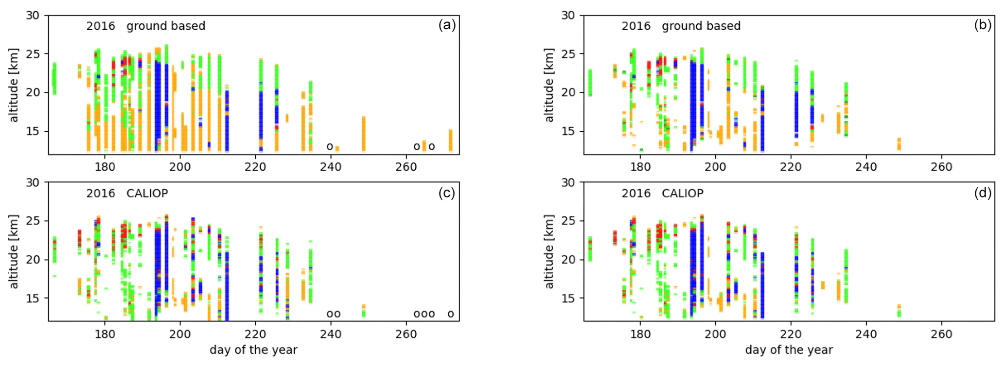
Figure 5All quasi-coincident observations (a, c) and only those where PSCs were observed by both lidars (b, d) for 2016 above Dome C. (a, b) Ground-based lidar. (c, d) CALIOP above Dome C. The different colors indicate PSCs of different composition. Green: NAT mixtures; yellow: STS; red: enhanced NAT mixtures; blue: ice. The circles indicate measured profiles without PSCs.
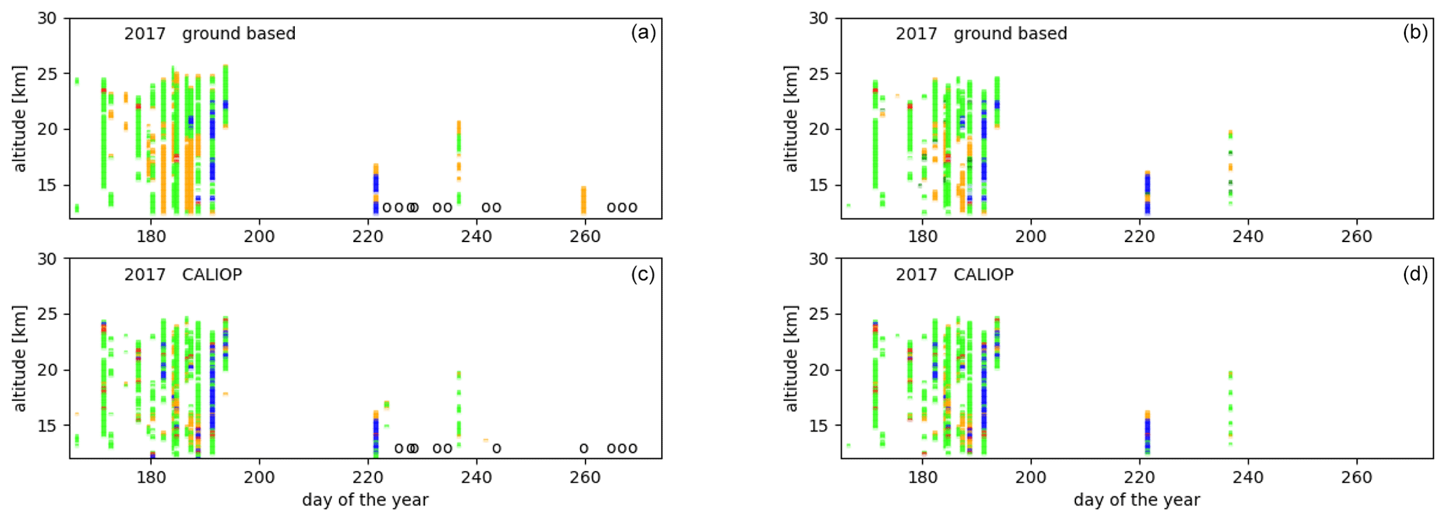
Figure 6All quasi-coincident observations (a, c) and only those where PSCs were observed by both lidars (b, d) for 2017 above Dome C. (a, b) Ground-based lidar. (c, d) CALIOP above Dome C. The different colors indicate PSCs of different composition. Green: NAT mixtures; yellow: STS; red: enhanced NAT mixtures; blue: ice. The circles indicate measured profiles without PSCs.
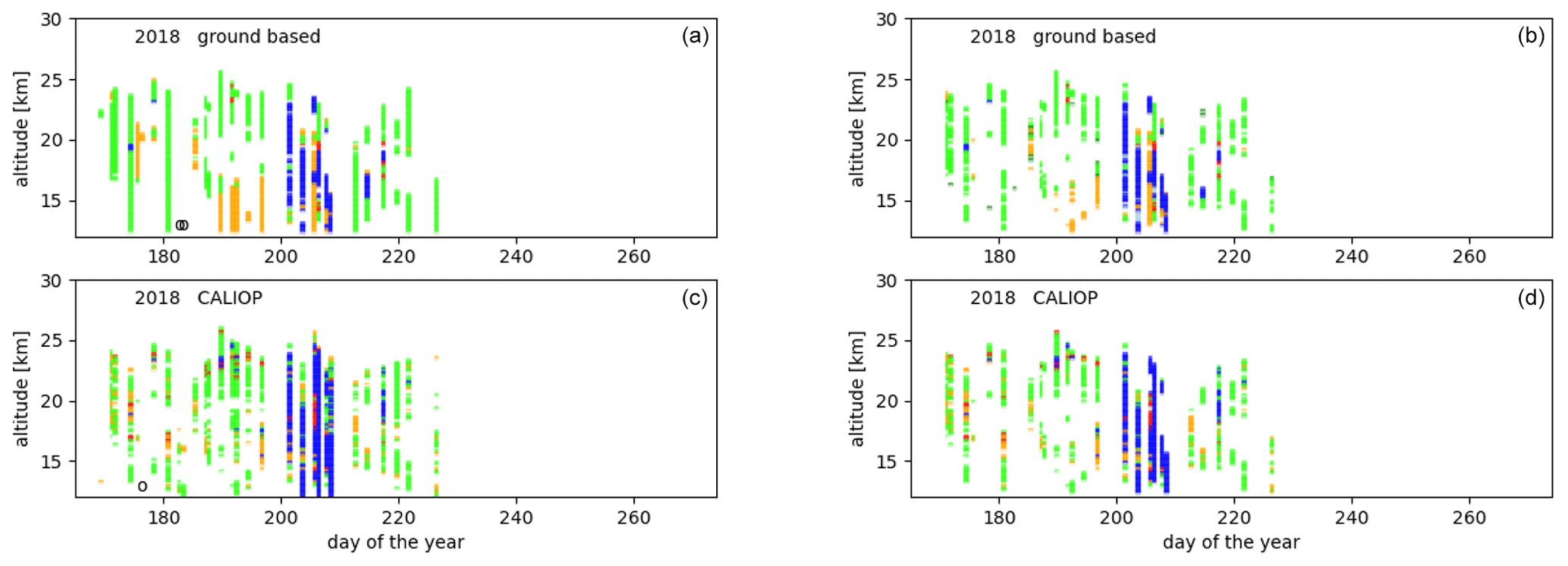
Figure 7All quasi-coincident observations (a, c) and only those where PSCs were observed by both lidars (b, d) for 2018 above Dome C. (a, b) Ground-based lidar. (c, d) CALIOP above Dome C. The different colors indicate PSCs of different composition. Green: NAT mixtures; yellow: STS; red: enhanced NAT mixtures; blue: ice. The circles indicate measured profiles without PSCs.
The dataset of all pixels of the quasi-coincident profiles consists of four categories of PSC detection: PSC detected by both ground-based and CALIOP lidars, no PSC detected by either ground-based or CALIOP lidar, PSC detected by the CALIOP lidar only, and PSC detected by the ground-based lidar only. The first two categories are listed in the column “detected” (see Table 1), because there is agreement between the (non)detection of a PSC. There is a small fraction (≈5 %) of coincidences where only CALIOP detects a PSC but a larger fraction (11 %–25 %) of coincidences where only the ground-based lidar detects a PSC. There are essentially three reasons for this. The first is that the ground-based lidar has on average a lower detection threshold; we found that Rthreshold has an average value of 1.08 for the ground-based lidar and 1.15 for CALIOP. This major sensitivity accounts for about 5 % to 10 % of the PSCs detected only by the ground-based lidar. The second is that we are not sure that the air masses observed by both lidars are part of the same large cloud. We expect that this does not occur frequently, since we have shown that around Dome C quite large PSC extension may be expected. The third is that a “hole” in the cloud deck is detected with a higher probability by CALIOP, since the observation time for a profile is only a few seconds, while the ground-based lidar integrates for about 30 min and thus observes a displacement of the cloud deck due to the wind. The frequency of holes in the cloud deck can be estimated from the analysis we performed on the CALIOP overpasses; about 10 % of all overpasses where PSCs were observed had a partial cloud cover (i.e along the track profiles with PSCs were observed as well as profiles without any PSC).
For comparison of PSC composition, we restrict the analysis to only those measurement pixels where both lidars detected a PSC (see the right columns of Figs. 4, 5, 6 and 7). The results of this comparison are reported in Table 3. The first four columns report the percentage of pixels with a certain PSC composition as determined by CALIOP. The columns under the header ground-based method 1 report the percentage of pixels where the ground-based lidar finds the same composition for that pixel. If we exclude 2014, on average about 60 % of the ground-based pixels show the same PSC composition as reported for CALIOP. NAT mixtures show the best agreement while the enhanced NAT mixtures observed by CALIOP are very often not observed as such by the ground-based lidar.
However, we want to explore how critically the PSC composition of the ground-based data depends on the choice of the thresholds, also considering that the calculated threshold for β⟂ in the classification of the ground-based data may be affected by instrumental errors, and RNAT|ice may also be slightly different at Dome C with respect to the value for the closest CALIOP profile. To take into account these uncertainties in both and RNAT|ice we allow a 10 % tolerance on both. This implies that all PSCs with a value of β⟂ between % are possibly STSs or NAT, and all PSCs with a value of the backscatter ratio R between % are possibly enhanced NAT mixtures or ice. This additional tolerance gives slightly better scores for the comparison (see Table 3, column ground-based method 2) but does not change the results in a significant way.
While performing ground-based measurements with a duration of several hours, we have observed that PSC layers may move up and down on the timescale of 30 min. Also, Achtert et al. (2011) observed a vertical shift in the cloud base of a PSC during a measurement campaign in the Arctic. Thus we also allowed a small vertical displacement of the air mass observed by the ground-based lidar with respect to the CALIOP observation, which is on average at a distance of 50 km from Dome C. This implies that each CALIOP pixel is now compared with three ground-based pixels, one at the same height and the other two at the next upper or lower layer (±180 m) (ground-based method 3). This last method leads to an improvement of about 10 % of the overall agreement and is shown in the column ground-based method 3 of Table 3. The largest effect can be observed for STSs and NAT mixtures. The last three columns in Table 3 report the sum of the pixels (for each of the four composition classes), where the ground-based lidar identifies the same composition as CALIOP, for each of the three methods applied.
Table 3The percentage of the different PSC composition classes are listed for CALIOP and ground-based observations following the three methods explained in the text. The last three columns are the percentages of correctly classified PSCs with respect to the CALIOP classification, according to the three methods.
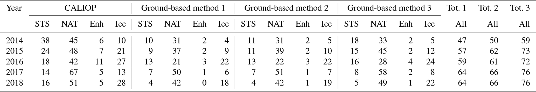
The results of the comparison show that on average for 58 % of all observations both lidars observe PSCs of the same composition, which becomes 71 % when tolerances on the thresholds are applied as well as on the altitude (±1 layer). NAT mixtures, being the dominant species, show an agreement better than 80 %, while ice and STSs are slightly worse. Significantly fewer enhanced NAT mixtures have been observed by the ground-based lidar with respect to CALIOP. A possible explanation might be that CALIOP may better resolve smaller patches of differing composition embedded within an otherwise homogeneous PSC, since its measurements are effectively an instantaneous “snapshot” along the orbit track. On the other hand, the ground-based lidar integrates over 30 min and averages the optical parameters used for the classification, thus promoting the NAT mixture classification, having intermediate values for the optical parameters with respect to the minor species, the latter producing the more extreme low or high values of the optical parameters. For instance if the ground-based lidar observes STSs for 10 min and NAT mixtures for 20 min, the average value of β⟂ will probably be higher than the detection threshold, and thus the observation will be classified as NAT mixtures, while CALIOP on the corresponding overpass track might identify both STSs and NAT mixtures, and the closest profile represents the statistical distribution of STSs and NAT mixtures. In any case, considering the expected composition homogeneity derived from the analysis made for all CALIOP overpasses in the box around Dome C (see Table 2), the overall result is satisfactory.
PSC occurrence and composition classification have been performed for all ground-based data and all satellite-borne lidar profiles at the shortest distance from Dome C (thus not limited to the quasi-coincident measurements), using detection and composition classification criteria as mentioned before. The ice frost temperature Tice and the formation temperature for NAT (nitric acid trihydrate), TNAT, have been calculated from local temperature, pressure, and H2O and HNO3 concentrations. Local temperatures and pressures have been taken from the ERA5 reanalysis dataset, while H2O and HNO3 concentrations are provided by the Microwave Limb Sounder (MLS). NAT PSCs form below TNAT, while STSs occur generally about 3∘ below TNAT, and water ice PSCs form below the ice frost temperature.
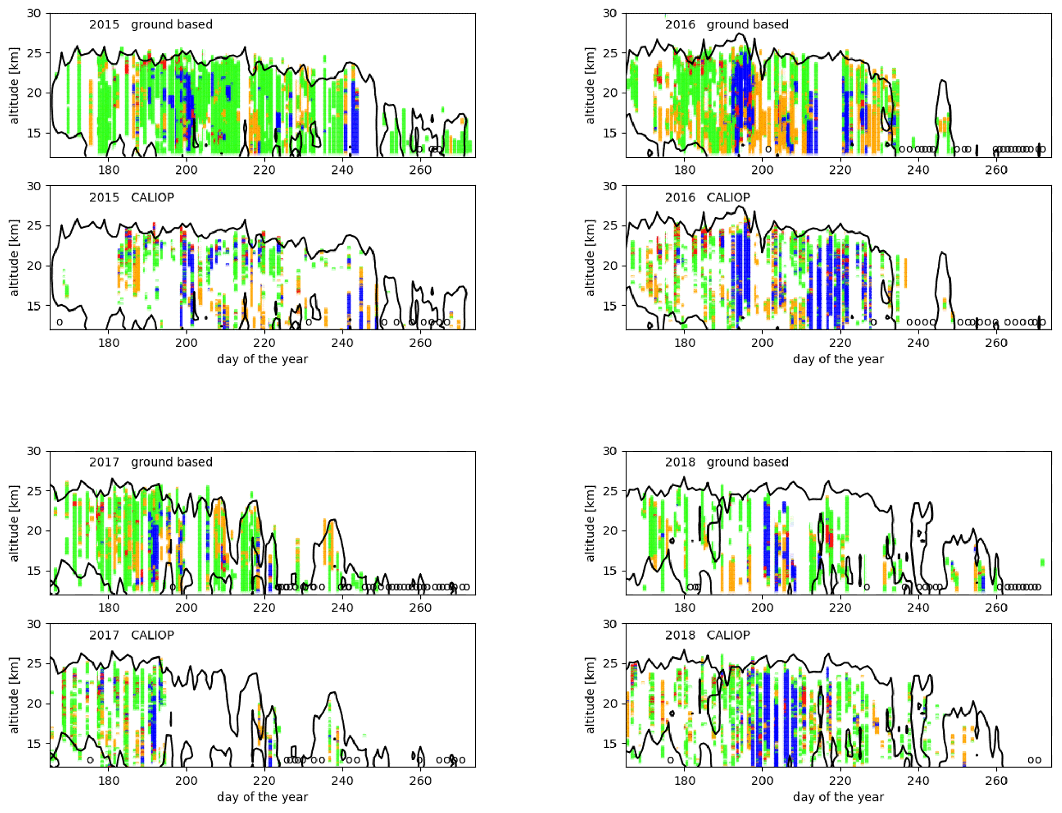
Figure 8All PSC observations for 2015–2018 above Dome C. Upper panels show ground-based lidar. Lower panels show CALIOP above Dome C. The different colors indicate classified PSCs. Green: NAT mixtures; yellow: STS; red: enhanced NAT mixtures; blue: ice. The circles indicate measured profiles without PSCs. The black contour indicates the area with a temperature below TNAT.
Figure 8 shows all ground-based measurements, the closest profile of all CALIOP overpasses within 100 km and contour plots indicating where the local temperature is below TNAT. It can be seen that PSCs are rarely observed at temperatures above TNAT. It is also clear that the temperature being below TNAT is not a sufficient condition to observe PSCs. Often PSC layers are separated by layers where neither of the two lidars observes PSCs. It is remarkable that the highest altitude where PSCs have been observed by the lidars coincides almost perfectly with the TNAT contour, which implies that the sensitivity of the ground-based lidar at Concordia station is generally not a limiting factor for the observations at high altitudes. It is also evident that from the second half of August Dome C is outside the coldest part of the vortex. This implies that ice and STS PSCs are seldom formed, while NAT occurrences are few. Looking at the previous figures, one can notice that CALIOP hardly observes any PSCs in September, while the ground-based lidar, being more sensitive due to the better ratio of the lidar signals and due to its longer integration times, as has been explained above, observes mostly NAT. In 2015 the vortex weakened only at the beginning of September, while in 2017 already around 10 August the local temperature between 12 and 30 km exceeded TNAT. Ice PSCs are mainly observed during the last 3 weeks of July, although a minor event can be observed at the end of August in 2015, and an important occurrence can be seen in the second week of August in 2016. We did not find evidence of a strong correlation with Tice contours. For all years very few PSCs have been observed in September. While the polar vortex has an almost circular symmetry around the South Pole during the winter, a displacement of the cold pool versus the Antarctic peninsula has been observed, starting from September and sometimes from the second half of August. Pitts et al. (2018) calculated 12-year (2006–2017) monthly means of PSC occurrence frequency at 20 km in the Southern Hemisphere and showed that these correlate strongly with contour maps of TNAT and Tice.
Lidar measurements of PSCs from the Dome C lidar observatory have been compared in terms of detection and composition with the data obtained with the spaceborne lidar CALIOP. In order to evaluate the ground-based lidar data, detection and composition classification algorithms have been developed, using criteria very similar to those used for the CALIOP data, taking into account systematic and statistical errors. Since exact coincidences are practically non-existent, quasi-coincident measurements have been defined as being recorded within 30 min of the CALIOP overpass and at the nearest distance from Dome C on each overpass, but in any case within 100 km. This implies a severe reduction of the available data but still resulted in a significant number of comparisons for every year. The validity of such a comparison, with quasi-coincidences, depends strongly on the uniformity of the PSC fields in the Dome C area. The hypothesis of sufficiently large horizontal extensions of the PSC clouds close to Dome C has been tested by considering all overpasses within a square of 200 km ×200 km centered on Dome C. A large number of overpasses with PSC detection resulted in being almost contiguous within the 200 km × 200 km box. This suggests that uniform PSC fields predominate in the area around Dome C. The detected PSC clouds might consist of PSCs of different composition (here we consider STSs, NAT mixtures, enhanced NAT mixtures and ice), interleaved both horizontally and vertically, and although the NAT mixtures are the dominant class during most of the winter, small patches of the minor species might be present. By studying the CALIOP composition classification along all overpasses at single altitude levels, it appeared that nearly half of all overpasses with PSCs showed contiguous layers of a single PSC class, while for about 25 % of the layers at least one-third minor species was found. This implies that while about half of the horizontal PSC fields have a homogeneous composition, a non-negligible part evidences the presence of PSCs with different composition within the Dome C area (200 km × 200 km). As a result we feel confident that a comparison between quasi-coincident measurements is fully justified for PSC detection and to a lesser extent for the composition classification. The comparisons are based on 5 years of data, from 2014 to 2018, and comprise 172 quasi-coincident vertical profiles.
The result of the detection comparison is that about 75 % of the (non-)PSCs were detected by both lidars, while about 5 % were detected only by CALIOP and 20 % only by the ground-based lidar. The latter is due to the better detection efficiency of the ground-based lidar and to the different integration times of the two lidars. The CALIOP observation is essentially a snapshot and has a higher probability of detecting holes in the cloud deck with respect to the ground-based lidar, which integrates over 30 min. If we consider only 2016, 2017 and 2018, these values are even better and reach 76 % to 84 % of agreement. The composition of the detected PSCs has been compared in a strict, pixel-to-pixel way, and also by introducing some more permissive criteria, such as a small variation in the classification thresholds and a comparison with the next higher or lower layer (±180 m). It can be concluded that the observation of NAT mixtures by CALIOP is confirmed in most cases (83 %) by the ground-based lidar, while the identification of the minor species by CALIOP was confirmed on average for 59 %, 32 % and 67 % of the cases, for STSs, enhanced NAT mixtures and ice, respectively, by the ground-based lidar. Our explanation is that the ground-based data acquisition produces averaged values of the optical constants, by integrating over 30 min, corresponding with a spatial integration of 15–30 km. This integration process favors the classification as NAT mixtures, at the cost of reducing classification of the other species. On the other hand CALIOP takes a snapshot during its overpass of about 30 s and is more sensitive to the other species.
The results presented here are providing a solid basis for the comparison of ground-based and spaceborne lidar observations of polar stratospheric clouds (PSCs). This is the most extensive comparison of such data, to our knowledge, and may provide a means to produce a standard PSC product for ground-based lidars, with a good compatibility with CALIOP and other spaceborne instruments, although with some caveats. It opens new possibilities of including ground-based validated PSC data in CCM models and microphysical studies. The method proposed here is shown to be valid for polar regions with rather uniform temperature fields and absence of important orographic structure but might be used with some constraints to different situations.
It has also been shown that observations obtained by the ground-based lidar and CALIOP are complementary and congruent and can be used to study seasonal and interannual variations in the presence of PSC clouds at Dome C. The PSCs observed by both systems are generally observed for local temperatures below TNAT, although some observations at higher temperatures are reported. These are mostly NAT mixtures that are known to persist some days even above TNAT. During the winter season, PSCs slowly descend and are rarely observed from the second half of August, in agreement with the warming of the vortex at Dome C.
For all 5 years concerned here, few PSCs have been observed during the second half of August and during September, most probably because of a displacement of the cold pool versus the Antarctic peninsula. Presently a climatological study for the Dome C area is underway by combining data of both lidars, which, based on this study, are compatible to a large degree.
The raw data of the ground-based lidar at Dome C are publicly available on the NDACC database (ftp://ftp.cpc.ncep.noaa.gov/ndacc/station/dome/ames/lidar/, Snels, 2019). The CALIOP v2 data are available from Michael Pitts and Lamont Poole on request.
MS was responsible for most of the writing, review and editing process, supported by all co-authors, with major contributions from FCo, FCa, LDL, MP and LP. The lidar data analysis was conducted by MS with contributions from AS, LDL and MDM. MDM installed the lidar at Dome C. FCo, MDM and LDL performed the calibration and maintenance of the ground-based lidar. MP and LP provided the CALIOP data and discussed the interpretation of the lidar data on many occasions.
The authors declare that they have no conflict of interest.
We also acknowledge the support of the ISSI-PSC initiative project. Logistical and wintertime technical support was provided by the Piano Nazionale della Ricerca in Antartide (PNRA). The authors thank Igor Petenko, Giampietro Casasanta, Simonetta Montaguti, Alfonso Ferrone, Filippo Cali Quaglia and Meganne Christian for performing the ground-based lidar measurements at Dome C during the winter and Maurizio Viterbini for his valuable technical support.
This research has been supported by the PNRA (grant nos. OSS-12 and 2009/B.08).
This paper was edited by Rolf Müller and reviewed by two anonymous referees.
Achtert, P. and Tesche, M.: Assessing lidar-based classification schemes for polar stratospheric clouds based on 16 years of measurements at Esrange, Sweden, J. Geophys. Res.-Atmos., 119, 1386–1405, https://doi.org/10.1002/2013JD020355, 2014. a
Achtert, P., Khosrawi, F., Blum, U., and Fricke, K. H.: Investigation of polar stratospheric clouds in January 2008 by means of ground-based and spaceborne lidar measurements and microphysical box model simulations, J. Geophys. Res.-Atmos., 116, D07201, https://doi.org/10.1029/2010JD014803, 2011. a, b
Adriani, A., Deshler, T., Gobbi, G. P., Johnson, B. J., and Di Donfrancesco, G.: Polar stratospheric clouds over McMurdo, Antarctica, during the 1991 spring: Lidar and particle counter measurements, Geophys. Res. Lett., 19, 1755–1758, https://doi.org/10.1029/92GL01941, 1992. a
Adriani, A., Deshler, T., Di Donfrancesco, G., and Gobbi, G.: Polar stratospheric clouds and volcanic aerosol during spring 1992 over McMurdo Station, Antarctica: Lidar and particle counter comparative measurements, J. Geophys. Res.-Atmos., 100, 25877–25897, 1995. a
Adriani, A., Massoli, P., Di Donfrancesco, G., Cairo, F., Moriconi, M., and Snels, M.: Climatology of polar stratospheric clouds based on lidar observations from 1993 to 2001 over McMurdo Station, Antarctica, J. Geophys. Res.-Atmos., 109, D24211, https://doi.org/10.1029/2004JD004800, 2004. a
Behrendt, A. and Nakamura, T.: Calculation of the calibration constant of polarization lidar and its dependency on atmospheric temperature, Opt. Express, 10, 805–817, https://doi.org/10.1364/OE.10.000805, 2002. a
Campbell, J. R. and Sassen, K.: Polar stratospheric clouds at the South Pole from 5 years of continuous lidar data: Macrophysical, optical, and thermodynamic properties, J. Geophys. Res.-Atmos., 113, D20204, https://doi.org/10.1029/2007JD009680, 2008. a
David, C., Bekki, S., Godin, S., Megie, G., and Chipperfield, M.: Polar stratospheric clouds climatology over Dumont d'Urville between 1989 and 1993 and the influence of volcanic aerosols on their formation, J. Geophys. Res.-Atmos., 103, 22163–22180, https://doi.org/10.1029/98JD01692, 1998. a
David, C., Keckhut, P., Armetta, A., Jumelet, J., Snels, M., Marchand, M., and Bekki, S.: Radiosonde stratospheric temperatures at Dumont d'Urville (Antarctica): trends and link with polar stratospheric clouds, Atmos. Chem. Phys., 10, 3813–3825, https://doi.org/10.5194/acp-10-3813-2010, 2010. a
David, C., Haefele, A., Keckhut, P., Marchand, M., Jumelet, J., Leblanc, T., Cenac, C., Laqui, C., Porteneuve, J., Haeffelin, M., Courcoux, Y., Snels, M., Viterbini, M., and Quatrevalet, M.: Evaluation of stratospheric ozone, temperature, and aerosol profiles from the LOANA lidar in Antarctica, Polar Sci., 6, 209–225, https://doi.org/10.1016/j.polar.2012.07.001, 2012. a
Di Liberto, L., Cairo, F., Fierli, F., Di Donfrancesco, G., Viterbini, M., Deshler, T., and Snels, M.: Observation of polar stratospheric clouds over McMurdo (77.85∘ S, 166.67∘ E) (2006–2010), J. Geophys. Res.-Atmos., 119, 5528–5541, https://doi.org/10.1002/2013JD019892, 2014. a
Fiocco, G., Cacciani, M., Di Girolamo, P., and Fua, D.: Stratospheric clouds at South-Pole during 1988 .1. Results of lidar observations and their relationship to temperature, J. Geophys. Res.-Atmos., 97, 5939–5946, 1992. a
Fua, D., Cacciani, M., Di Girolamo, P., Fiocco, G., and Disarra, A.: Stratospheric clouds at South-Pole during 1988 .2. Their evolution in relation to atmospheric structure and composition, J. Res.-Atmos., 97, 5947–5952, 1992. a
Gobbi, G.: Lidar estimation of stratospheric aerosol properties – surface, volume, and extinction to backscatter ratio, J. Geophys. Res.-Atmos., 100, 11219–11235, https://doi.org/10.1029/94JD03106, 1995. a
Hanson, D. and Mauersberger, K.: Laboratory studies of the nitric acid trihydrate: Implications for the south polar stratosphere, Geophys. Res. Lett., 15, 855–858, https://doi.org/10.1029/GL015i008p00855, 1988. a
Huang, W., Chu, X., Simpson, S. E., Nott, G. J., and Espy, P. J.: Polar Stratospheric Clouds Observed by Lidar in Antarctica and the Effect of Polar Vortex, AGU Spring Meeting Acapulco, Guerrero, Mexico, 22–25 May 2007, Eos Trans. AGU, 88, Jt. Assembly. Suppl., Abstract A53A-07, 2007. a
Hunt, W. H., Winker, D. M., Vaughan, M. A., Powell, K. A., Lucker, P. L., and Weimer, C.: CALIPSO lidar description and performance assessment, J. Atmos. Ocean. Tech., 26, 1214–1228, https://doi.org/10.1175/2009JTECHA1223.1, 2009. a
Klett, J. D.: Stable analytical inversion solution for processing lidar returns, Appl. Optics, 20, 211–220, https://doi.org/10.1364/AO.20.000211, 1981. a
Pitts, M. C., Poole, L. R., and Thomason, L. W.: CALIPSO polar stratospheric cloud observations: second-generation detection algorithm and composition discrimination, Atmos. Chem. Phys., 9, 7577–7589, https://doi.org/10.5194/acp-9-7577-2009, 2009. a
Pitts, M. C., Poole, L. R., Dörnbrack, A., and Thomason, L. W.: The 2009–2010 Arctic polar stratospheric cloud season: a CALIPSO perspective, Atmos. Chem. Phys., 11, 2161–2177, https://doi.org/10.5194/acp-11-2161-2011, 2011. a
Pitts, M. C., Poole, L. R., Lambert, A., and Thomason, L. W.: An assessment of CALIOP polar stratospheric cloud composition classification, Atmos. Chem. Phys., 13, 2975–2988, https://doi.org/10.5194/acp-13-2975-2013, 2013. a
Pitts, M. C., Poole, L. R., and Gonzalez, R.: Polar stratospheric cloud climatology based on CALIPSO spaceborne lidar measurements from 2006 to 2017, Atmos. Chem. Phys., 18, 10881–10913, https://doi.org/10.5194/acp-18-10881-2018, 2018. a, b, c, d
Santacesaria, V., MacKenzie, A. R., and Stefanutti, L.: A climatological study of polar stratospheric clouds (1989–1997) from LIDAR measurements over Dumont d'Urville (Antarctica), Tellus B, 53, 306–321, https://doi.org/10.1034/j.1600-0889.2001.01155.x, 2001. a
Simpson, S. E., Chu, X., Liu, A., Robinson, W., J. Nott, G., Diettrich, J., Espy, P., and Shanklin, J.: Polar stratospheric clouds observed by a lidar at Rothera, Antarctica (67.5∘ S, 68.0∘ W), in: SPIE Proceedings volume 5887, Optics and Photonics 2005, 31 July–4 August 2005, San Diego, California, United States, https://doi.org/10.1117/12.620399, 2005. a
Snels, M.: Ground-based lidar data at Dome C, list of monthly files, NDACC database, available at: ftp://ftp.cpc.ncep.noaa.gov/ndacc/station/dome/ames/lidar/ (last access: 11 February 2021), 2019. a, b
Snels, M., Cairo, F., Colao, F., and Di Donfrancesco, G.: Calibration method for depolarization lidar measurements, Int. J. Remote Sens., 30, 5725–5736, https://doi.org/10.1080/01431160902729572, 2009. a
Snels, M., Scoccione, A., Di Liberto, L., Colao, F., Pitts, M., Poole, L., Deshler, T., Cairo, F., Cagnazzo, C., and Fierli, F.: Comparison of Antarctic polar stratospheric cloud observations by ground-based and space-borne lidar and relevance for chemistry–climate models, Atmos. Chem. Phys., 19, 955–972, https://doi.org/10.5194/acp-19-955-2019, 2019. a, b, c, d, e
Stephens, G., Winker, D., Pelon, J., Trepte, C., Vane, D., Yuhas, C., L'Ecuyer, T., and Lebsock, M.: CloudSat and CALIPSO within the A-Train: Ten years of actively observing the Earth system, B. Am. Meteorol. Soc., 99, 569–581, https://doi.org/10.1175/BAMS-D-16-0324.1, 2018. a
Stephens, G. L., Vane, D. G., Boain, R. J., Mace, G. G., Sassen, K., Wang, Z., Illingworth, A. J., O'Connor, E. J., Rossow, W. B., Durden, S. L., Miller, S. D., Austin, R. T., Benedetti, A., Mitrescu, C., and Team, T. C. S.: The cloudsat mission and the A-train, B. Am. Meteorol. Soc., 83, 1771–1790, https://doi.org/10.1175/BAMS-83-12-1771, 2002. a
Tesche, M., Achtert, P., and Pitts, M. C.: On the best locations for ground-based polar stratospheric cloud (PSC) observations, Atmos. Chem. Phys., 21, 505–516, https://doi.org/10.5194/acp-21-505-2021, 2021. a, b
Waugh, D. W. and Randel, W. J.: Climatology of Arctic and Antarctic Polar Vortices Using Elliptical Diagnostics, J. Atmos. Sci., 56, 1594–1613, https://doi.org/10.1175/1520-0469(1999)056<1594:COAAAP>2.0.CO;2, 1999. a
Winker, D. M., Vaughan, M. A., Omar, A., Hu, Y., Powell, K. A., Liu, Z., Hunt, W. H., and Young, S. A.: Overview of the CALIPSO mission and CALIOP data processing algorithms, J. Atmos. Ocean. Tech., 26, 2310–2323, https://doi.org/10.1175/2009JTECHA1281.1, 2009. a
- Abstract
- Introduction
- PSC observations at Dome C by ground-based and satellite-borne lidar
- Comparison of PSCs as observed and classified by ground-based and satellite-borne lidar
- PSC occurrence as observed and classified by ground-based and satellite-borne lidar
- Conclusions
- Data availability
- Author contributions
- Competing interests
- Acknowledgements
- Financial support
- Review statement
- References