The response of mesospheric H₂O and CO to solar irradiance variability in models and observations

Water vapor (H₂O) is the source of reactive hydrogen radicals in the middle atmosphere, whereas carbon monoxide (CO), being formed by CO₂ photolysis, is suitable as a dynamical tracer. In the mesosphere, both H₂O and CO are sensitive to solar irradiance (SI) variability because of their destruction/production by solar radiation. This enables us to analyze the solar signal in both models and observed data. Here, we evaluate the mesospheric H₂O and CO response to solar irradiance variability using the Chemistry-Climate Model Initiative (CCMI-1) simulations and satellite observations. We analyzed the results of four CCMI models (CMAM, EMAC-L90MA, SOCOLv3, and CESM1-WACCM 3.5) operated in CCMI reference simulation REF-C1SD in specified dynamics mode, covering the period from 1984–2017. Multiple linear regression analyses show a pronounced and statistically robust response of H₂O and CO to solar irradiance variability and to the annual and semiannual cycles. For periods with available satellite data, we compared the simulated solar signal against satellite observations, namely the GOZCARDS composite for 1992–2017 for H₂O and Aura/MLS measurements for 2005–2017 for CO. The model results generally agree with observations and reproduce an expected negative and positive correlation for H₂O and CO, respectively, with solar irradiance. However, the magnitude of the response and patterns of the solar signal varies among the considered models, indicating differences in the applied chemical reaction and dynamical schemes, including the representation of photolyzes. We suggest that there is no dominating thermospheric influence of solar irradiance in CO, as reported in previous studies, because the response to solar variability is comparable with observations in both low-top and high-top models. We stress the importance of this work for improving our understanding of the current ability and limitations of state-of-the-art models to simulate a solar signal in the chemistry and dynamics of the middle atmosphere.

1 Introduction

H₂O plays an important role in atmospheric chemistry as a source of the hydrogen oxide radicals (HO_x), which are important for ozone loss. There are two main sources of water vapor in the middle atmosphere. The first is a direct carry-over of H₂O through the tropopause tropical cold trap (∼ 2–3 ppmv), where strong dehydration of air occurs (Nicolet, 1981). The second is indirect, namely the upward stratospheric transport of CH₄ and its subsequent oxidation. The main chemical reaction leading to H₂O formation throughout the atmosphere is from methane oxidation (Wofsy et al., 1972):

$$\begin{array}{}\text{(1)}& {\mathrm{CH}}_{\mathrm{4}}+{\mathrm{OH}}^{\mathrm{•}}\to {{\mathrm{CH}}_{\mathrm{3}}}^{\mathrm{•}}+{\mathrm{H}}_{\mathrm{2}}\mathrm{O}.\end{array}$$

Middle atmospheric trends in H₂O are largely determined by changes in the tropospheric content of CH₄ and temperature in the tropical tropopause (Nedoluha et al., 2013). The amount of H₂O in the middle atmosphere can reach a value of up to 10 ppmv (Brasseur and Solomon, 2005). In the mesosphere where the CH₄ is fully oxidized, the H₂O can have an amount of about 6.6 ppmv. Nevertheless, the highest mixing ratio of H₂O is in the lower atmosphere with 10–100 ppm in the upper and more than 10 000 ppm in the lower troposphere (Palchetti et al., 2008). With increasing altitude in the mesosphere, the photodissociation of H₂O is caused by solar irradiance (SI) at the Ly-α (121.25 nm) spectral line of hydrogen and within the spectral range of the oxygen Schumann–Runge continuum (175–200 nm; Frederick and Hudson, 1980). The photodissociation lifetime of water vapor in the presence of the solar Ly-α radiation below the mesopause is estimated to be less than 200 h (Kingston, 1987) because J_(Ly-α) of (H₂O) equals $\mathrm{1.6}\times {\mathrm{10}}^{-\mathrm{6}}$ s⁻¹ for a total number of O₂ molecules of about 10²⁰ cm⁻². Products of H₂O photolysis are atomic hydrogen and hydroxyl radicals:

$$\begin{array}{}\text{(R1)}& {\mathrm{H}}_{\mathrm{2}}\mathrm{O}+h\mathit{\nu }\to {\mathrm{H}}^{\mathrm{•}}+{\mathrm{OH}}^{\mathrm{•}}.\end{array}$$

As such, an anticorrelation of water vapor with solar irradiance, with the strongest response in the mesosphere, is expected (Chandra et al., 1997; Hervig and Siskind, 2006; Shapiro et al., 2012), and the strength of this effect depends upon the intensity of solar irradiance in the Ly-α line and the Schumann–Runge band.

Carbon monoxide (CO) is widely present in the lower thermosphere and mesosphere, and due to its chemical lifetime of more than 1 month, it can be used for investigating transport processes in the middle atmosphere. CO can react with some species (e.g., OH^•) which would otherwise destroy ozone and CH₄, enhancing its radiative forcing (Ryan et al., 2018). Contrary to H₂O, CO is positively correlated with solar irradiance as it is primarily formed through the photolysis of CO₂ in the lower thermosphere and upper mesosphere at Ly-α (Wofsy et al., 1972) as follows:

$$\begin{array}{}\text{(2)}& {\mathrm{CO}}_{\mathrm{2}}+h\mathit{\nu }\to \mathrm{CO}+\mathrm{O}.\end{array}$$

In the troposphere, the main source of CO is the oxidation of hydrocarbons (Minschwaner et al., 2010). However, in the mesosphere the amount of CO from the oxidation of CH₄ and isoprene is so much smaller compared to the CO₂ photodissociation (Eq. 2) that this process can be neglected at high altitudes (Garcia et al., 2014). The chemical loss of CO in the atmosphere occurs by oxidation (Levy, 1971):

$$\begin{array}{}\text{(3)}& \mathrm{CO}+{\mathrm{OH}}^{\mathrm{•}}\to {\mathrm{CO}}_{\mathrm{2}}+{\mathrm{H}}^{\mathrm{•}}.\end{array}$$

The amount of CO in the mesosphere is estimated to be within 30 ppb–10 ppm (Brasseur and Solomon, 2005) and 50–100 ppb in the uncontaminated air in the troposphere (Minschwaner et al., 2010), having a strong vertical gradient. Mesospheric concentrations of H₂O and CO are strongly determined by the solar irradiance. Since the processes leading to H₂O∕CO destruction/production are much faster than changes in solar irradiance on all timescales, we can assume they are essentially linear. Therefore, an attribution approach using multiple linear regression (MLR) analysis is reasonable to estimate the impact of solar irradiance on H₂O and CO variability in the middle atmosphere. We apply this linear statistical tool to different model and satellite data. One major goal of this study is to compare the modeled solar signal in mesospheric H₂O and CO to observations. Recently, the photochemical H₂O loss by Ly-α radiation in UARS/HALOE (Upper Atmosphere Research Satellite/Halogen Occultation Experiment) measurements was estimated to be about 35 % at 0.01 hPa (∼ 80 km altitude) at 50^∘ N using MLR (Remsberg et al., 2018). Tropical tendencies in mesospheric water vapor using MLR analysis of Aura/MLS (Microwave Limb Sounder) observations for the 2004–2015 period were presented by Nath et al. (2018). Their analysis showed a pronounced trend in water vapor throughout the whole considered period, as well as a strong negative correlation with the F10.7 solar index that maximizes at 0.01 hPa (−0.56 ppmv 1 %⁻¹ of Ly-α). A solar signal in lower stratospheric H₂O was investigated by Schieferdecker et al. (2015). Using MLR, they showed a negative correlation between H₂O and solar activity with a phase shift of about 2 years in composite data of HALOE and MIPAS (Michelson Interferometer for Passive Atmospheric Sounding) over 60^∘ N–60^∘ S.

Lee et al. (2013) presented a study of the middle atmospheric CO variation caused by solar irradiance changes using MLS and solar irradiance measurements from the Solar Radiation and Climate Experiment (SORCE). Their results reveal a significant positive correlation of up to 0.6 between solar irradiance and CO variation in the mesosphere, as well as downward transport of the CO anomaly induced by solar irradiance over high latitudes with a descent rate of about 1.3 km d⁻¹. Lee et al. (2018) expanded their previous work and investigated the solar cycle variation in CO using MLS measurements for 2004–2017, as well as free-running WACCM (Whole Atmosphere Community Climate Model) simulations using two different solar spectral irradiance datasets. The updated results have a higher correlation (up to 0.8) and show that 68 % of upper mesospheric CO variation is caused by solar irradiance changes, as well as pronounced downwelling of the signal within the polar vortex regions. The results simulated with WACCM (3.5) underestimate the CO variation in the upper mesosphere by a factor of 3 compared to the Aura/MLS observations. However, here it should be mentioned that the applied WACCM version does not employ the extreme ultraviolet (EUV) photolysis and reaction by CO₂ with O⁺ as an additional CO production mechanism in the thermosphere. The modeled CO distribution with WACCM version 4.0 shows CO in better agreement with the MIPAS and ACE-FTS (Atmospheric Chemistry Experiment Fourier Transform Spectrometer) observations (Garcia et al., 2014). This also could cause some issues when comparing the results of models for which this production mechanism is not included. Thus, the results of previous studies revealed issues in the modeling of the influence of solar irradiance and motivate an intercomparison analysis of multiple models and observations. So far, an MLR analysis using multiple chemistry-climate models (CCMs) and observations of both CO and H₂O has not been conducted.

In this work, we present an MLR analysis of simulations with several chemistry-climate models in specified dynamics mode for the period 1984–2017, as well as available observations from UARS/HALOE (1992–2005) and Aura/MLS (2005–2017), which provide data for 26 years with a good resolution and without serious gaps. The combined UARS/HALOE and Aura/MLS records provide observations of CO (only for the Aura/MLS period) and H₂O (for the whole 1992–2017 period), which makes these data suitable for our analysis. The MLR method is used to retrieve H₂O and CO responses to solar irradiance variability and to estimate the consistency of the solar signal in CCMs to that found in observations and between CCMs. Analyzing the differences in the solar responses can reveal potential model limitations, such as the dynamics of the middle atmosphere (weak or strong transport), the presence of thermospheric sources (important since some models have an upper boundary at 0.01 hPa), and the photochemistry and chemical production or loss of the species considered here. H₂O and CO were chosen as they are very sensitive to solar irradiance variations in the mesosphere (Remsberg et al., 2018; Lee et al., 2018), making them good candidates for this kind of analysis.

In Sect. 2, we describe the datasets used in this study. Section 3 briefly describes the MLR model setup used to retrieve the solar signal response. The results of the MLR analysis of the CMAM, EMAC-L90MA (hereinafter denoted as EMAC), SOCOLv3 (hereinafter denoted as SOCOL), and WACCM REF-C1SD model runs for the entire period 1984–2017, as well as the comparison with H₂O measurements from UARS/HALOE and Aura/MLS for the 1992–2017 period and CO measurements from Aura/MLS for the 2005–2017 period, are presented in Sect. 4. The discussion and overall summary can be found in Sects. 5 and 6.

2 Datasets

For our study, we chose four global climate models involved in the Chemistry-Climate Model Initiative (CCMI-1) project. The CCMI project aims at carrying out the inter-model comparison and validation of model results with observations¹. For the analysis, we used the results of the REF-C1SD experiment which was performed using boundary conditions extracted from observations, including the atmospheric level of greenhouse gases and ozone-depleting substances (ODSs), as well as sea surface temperature and sea ice concentration (Morgenstern et al., 2017). Specified dynamics (SD) here means that meteorological fields in the model experiments are nudged toward reanalysis datasets. The nudging is applied in CCMI-1 models for different atmospheric regions, as well as using different reanalysis data (see Table 1; Chrysanthou et al., 2019). The selection of models was based on the inspection of the simulated H₂O and CO time series for the presence of the solar signal in the mesosphere and on data reliability. Careful analysis of the CCMI-1 results showed that only CMAM, EMAC, SOCOL, and WACCM CCMs are suitable for the intended analysis, while other models involved in CCMI-1 were either in an unusable format, did not extend high enough, or lacked any solar signal in H₂O and CO. The REF-C1SD simulations of the four chosen models were extended to 2017 (CCMI-1 is until 2011) to overlap with the recent satellite measurements.

Scinocca et al. (2008)Jöckel et al. (2010)Jöckel et al. (2016)Stenke et al. (2013)Revell et al. (2015)Marsh et al. (2013)Verronen et al. (2016)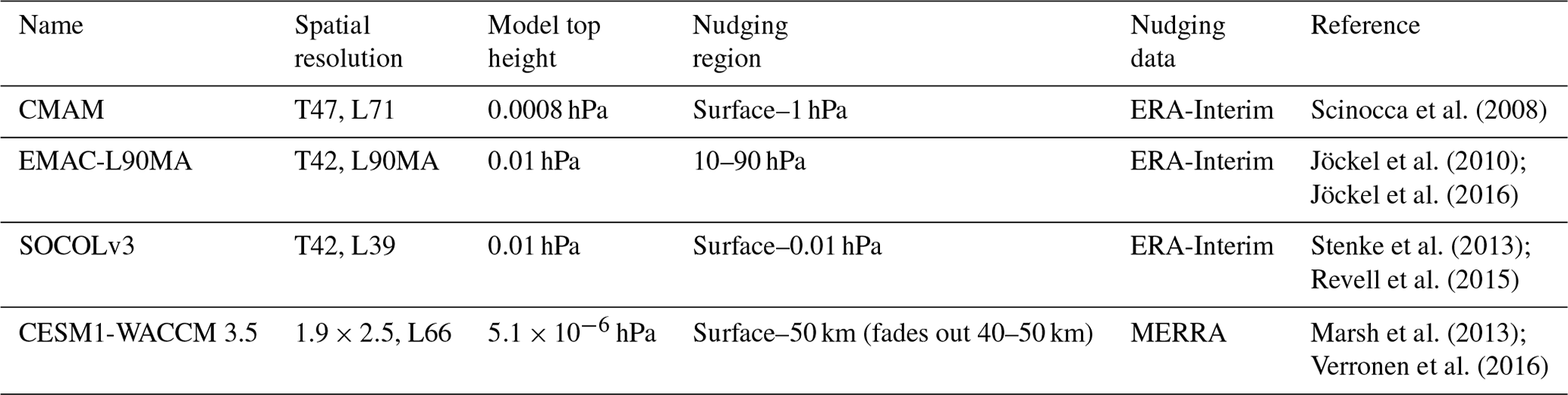

Table 1 CCMI-1 model setup.

We focus on mesospheric altitudes for the examination of the solar signal response in atmospheric chemistry. Thus, differences in nudging setups play no role as the mesosphere does not undergo direct nudging. There is an exception for SOCOL in that it is the only model for which the whole model atmosphere is nudged up to the 0.01 hPa level. Additionally, in the frame of this work, it is important to describe the lower limit of the wavelength for photolysis and photoionization in CCMI-1 models presented in Table 1.

In EMAC, for the simulation considered in this work, the photolysis rates have been calculated with the submodel JVAL (Sander et al., 2014), which uses eight wavelength bands ranging from 178.6 to 682.5 nm (Landgraf and Crutzen, 1998) and includes a parametrization for Ly-α photolysis (Chabrillat and Kockarts, 1997). In SOCOL, photolysis rates are calculated using a lookup table approach (Rozanov et al., 1999), including effects of the solar irradiance variability with the lower limit for photolysis at 120 nm. In the CMAM model, the shortest wavelength is 121.0 nm. Also, the parameterization for NO photolysis from Minschwaner and Siskind (1993) is used; however, there is no effect of solar variability included on this rate. In WACCM, the photolysis of H₂O starts at Ly-α (121.5 nm). Fluxes at that wavelength are calculated using the Chabrillat and Kockarts (1998) scheme. For Eq. (2), cross sections from 0.5 to 105.0 nm in the EUV and X-ray wavelength region are used. Solar fluxes are calculated with Solomon and Qian (2005). Additionally, in WACCM, an ion chemistry loss for CO₂ is included: ${\mathrm{CO}}_{\mathrm{2}}+{\mathrm{O}}^{+}\to {\mathrm{O}}_{\mathrm{2}}^{+}+\mathrm{CO}$. In the other models (EMAC, CMAM, and SOCOL) considered here, ion chemistry is not included.

Since time series of H₂O and CO from CMAM, SOCOL, WACCM, and EMAC SD simulations are available until 2017, we compare the solar response with observations from Aura/MLS CO for the available period of 2005–2017 and H₂O for 1992–2017. However, to extend the REF-C1SD simulations of SOCOL and EMAC, the NRLSSI data (Lean et al., 2005) for REF-C1 was used only until 2011, and onward the models used the boundary conditions (greenhouse gases and ODSs) of the RCP6.0 scenario (REF-C2). In EMAC, the conditions for the year 2011 have been cyclically repeated for the years 2012–2017. In the case of solar forcing, EMAC uses the adapted solar forcing according to the one used in the HadGEM2-ES CMIP5 6.0 simulation (Jones et al., 2011). The CMAM data for the considered period were from a different specified dynamics simulation than the one submitted to CCMI-1, produced using a method identical to that of nudging with reanalysis but with specified stratospheric aerosols, extraterrestrial solar flux, and emissions from datasets specified for CMIP6 (Eyring et al., 2016). For the extension of the WACCM time series of both H₂O and CO, the NRLSSI2 model (Coddington et al., 2016) is used from 2015 onward.

To compare simulated results, the observations of H₂O from the Halogen Occultation Experiment HALOE (1992–2005) on board the Upper Atmosphere Research Satellite (UARS), and the observations of H₂O and CO from the Microwave Limb Sounder (MLS) (2005–2017) instrument on board the Aura satellite were analyzed. HALOE measured the reduction in the intensity of solar energy that passes through the atmosphere to obtain the gas concentration of important atmospheric trace gases. A detailed HALOE instrument description can be found in Russell et al. (1993). The principal method used with the MLS instrument is the measurement of microwave thermal emissions from the atmosphere to remotely obtain profiles of different atmospheric constituents. More information on MLS can be found in Waters et al. (2006). For the analysis of H₂O, we used a combination of the GOZCARDS merged dataset consisting of all available data for the 1992–2004 period (Anderson et al., 2013) and data from ongoing missions of MLS (Waters et al., 2006) and ACE-FTS (Bernath et al., 2005) for 2005–2017 obtained using an averaging procedure based on overlap periods. Carbon monoxide time series are available only for the period 2005–2017 (Bernath et al., 2005; Waters et al., 2006). Both datasets of observations are binned into 20 latitude zones since data of observations (especially HALOE) are rather noisy, and a linear gap-filling procedure was applied to produce a continuous time series.

Figure 1 shows the time series of H₂O and CO averaged over the tropics (30^∘ N–30^∘ S) at 0.01 hPa from CCMI-1 REF-C1SD simulations and observations from the GOZCARDS composite and Aura/MLS instruments.

Figure 1 Time series of monthly mean (a) H₂O and (b) CO mixing ratio from CCMI-1 models, as well as GOZCARDS observational composite (gray line and shading in a, starting in 1992) and Aura/MLS observations (blue line and shading in b, starting in 2005) at 0.01 hPa averaged over the tropics (30^∘ N–30^∘ S). Shadings: 1σ standard deviation. The dash-dotted red line indicates the F10.7 solar index.

It should be mentioned that the upper boundary for SOCOL and EMAC at 0.01 hPa belongs to the sponge layer where high diffusion is used to avoid excessive wave amplitudes. The importance for chemistry is that a zero-flux condition is applied for SOCOL and EMAC, which means that H₂O and CO concentrations are not prescribed at the 0.01 hPa level. For WACCM and CMAM, the model's top level is above 0.01 hPa (at $\mathrm{5.1}\times {\mathrm{10}}^{-\mathrm{6}}$ hPa and 0.0008 hPa, respectively), and the influx of the air with rather high CO and low H₂O concentrations from the lower thermosphere could play an important role. For visualization purposes, we smooth H₂O and CO time series presented in Fig.1 using the third-order polynomial interpolation with a 2-year length of the averaging window; however, data used later for MLR analysis are taken in their original form without smoothing. As shown in Fig. 1, there is a pronounced response of H₂O and CO to solar irradiance variability, represented here as the F10.7 solar radio flux (right vertical axis). In the case of H₂O, there is a decrease in mixing ratio during a solar activity maximum and the opposite for CO, which is enhanced during the solar maximum. Obviously, the amplitude of the solar signal in H₂O and CO and their mean values are not the same in different models and observations. The comparison of H₂O mixing ratios in Fig. 1 during the 1984–2017 period reveals that all models except SOCOL are within the standard deviation of the merged observational data. The observed H₂O mixing ratio is slightly overestimated by EMAC and underestimated by CMAM and WACCM. A substantial overestimation of the water vapor loss by photolysis in SOCOL may lead to an underestimation of the mixing ratio by up to 50 % (Sukhodolov et al., 2017). This can have implications for the simulations of HO_x and ozone loss in the mesosphere. In the case of CO, SOCOL, and WACCM, results are almost identical and in good correspondence with Aura/MLS observations during 2005–2017. This agreement suggests that the influx of CO from the thermosphere in WACCM does not substantially contribute to CO in the tropics. However, in SOCOL, the lack of downward transport from the thermosphere might hypothetically be compensated for by erroneous, for instance too strong, in situ production in the upper mesosphere. On the other hand, the absolute values of the CO mixing ratio in EMAC and CMAM are very similar. They are underestimated by a factor of 2 though in comparison to Aura/MLS data, which might be due to an underestimated production. Thus, it is obvious that H₂O and CO behave differently in models and observations, subject to the exact treatment of chemistry and radiation in the models. In the following, a detailed MLR analysis of modeled H₂O and CO, as well as of the observational datasets, will be presented.

3 Description of the MLR model

The multiple linear regression (MLR) model used in this study is based on the x regression tool (Kuchar, 2016) consisting of the Python statistical models library statsmodels (Seabold and Perktold, 2010) coupled with the xarray package dealing with multidimensional arrays (Hoyer and Hamman, 2017). This model configuration adopts a well-established attribution methodology already used in previous studies (Ball et al., 2016; Kuchar et al., 2017). In this version, the MLR model uses nine explanatory/predictor variables and one response variable which is either H₂O or CO, respectively. As predictors, we use the solar F10.7 index (in solar flux units), the El Niño–Southern Oscillation (ENSO) ERSST v5 Nino4 index (in kelvin), zonal winds at 30 and 50 hPa (in m s⁻¹) as proxies of quasi-biennial oscillation (QBO) assuming their orthogonality (Crooks and Gray, 2005), and stratospheric aerosol optical depth (SAOD; dimensionless), as well as two annual (AO) and two semiannual (SAO) oscillation harmonics. To remove the residual autocorrelation, a second-order autocorrelation (AR2) model is used in an iterative way. The time series of the monthly mean response variables Y(t) (in ppmv), reconstructed as a function of time (t) by the MLR model for every single cell (latitude × pressure level), is as follows:

$$\begin{array}{}\text{(4)}& \begin{array}{rl}Y\left(t\right)& =\mathit{\alpha }+\mathit{\beta }\mathrm{SOLAR}\left(t\right)+\mathit{\gamma }\mathrm{ENSO}\left(t\right)+{\mathit{\delta }}_{\mathrm{1}}\mathrm{QBO}\mathrm{30}\left(t\right)\\ & +{\mathit{\delta }}_{\mathrm{2}}\mathrm{QBO}\mathrm{50}\left(t\right)+\mathit{ϵ}\mathrm{SAOD}\left(t\right)\\ & +\mathrm{2}-\mathit{\zeta }\mathrm{AO}\left(t\right)+\mathrm{2}-\mathit{\eta }\mathrm{SAO}\left(t\right)\\ & +\mathit{\theta }\mathrm{TREND}\left(t\right)+e\left(t\right).\end{array}\end{array}$$

To estimate the statistical significance of the derived regression coefficients to approximate Y(t), we use a t test with 95 % confidence level taking into account the residual autocorrelation. In Eq. (4), e(t) means the stochastic noise of the model when AR2 is included. All explanatory variables with a monthly resolution were taken from the KNMI Climate Explorer database². In our study, the regression coefficients for the solar proxy (β) are estimated using the MLR model as a latitude-altitude matrix, and they are used to calculate the solar signal as (Y_s ∕ $\stackrel{\mathrm{‾}}{Y}$) × 100 %, where $\stackrel{\mathrm{‾}}{Y}$ is an averaged H₂O∕CO (ppmv) for the whole considered period and $Y_{\mathrm{s}}=\mathit{\beta }\times \mathrm{100}$ is H₂O∕CO change (ppmv) caused by F10.7 change by 100 units. As such we estimate the percentage change in H₂O and CO induced by solar irradiance changes from the minimum to the maximum of the 11-year solar cycle. To check how much of the total variability is represented by the solar variability and whether our choice of regressors is justified, we calculate the relative importance (RI) of each regressor. We use the Lindeman–Merenda–Gold measure (LMG; Lindeman et al., 1980) to decompose R² (coefficient of determination) and to determine RI, which refers to the proportionate contribution each predictor variable makes to the total predicted criterion variance. Figure 2 shows RI distributions of zonally averaged time series of CO and H₂O at 0.01 hPa between 30^∘ S and 30^∘ N for the period 2005–2017 and 1992–2017, respectively. Our MLR model, including annual and semiannual harmonics, can assess 70 %–90 % of the total variability (shown as “total” on the right-hand side of both panels in Fig. 2). The solar variability represents around 10 % of the total variance, and it is the strongest after the SAO (∼ 50 %) driver of CO and H₂O variability in all model data and observations around the Equator at 0.01 hPa. While the solar RI in the CO time series of EMAC agrees well with the Aura/MLS observations, CMAM and SOCOL overestimate and WACCM underestimates the solar variability. It is worth saying that in some models, AO and SAO in the upper mesosphere may experience some issues as much of the variability on those timescales comes from the residual circulation that would not be fully resolved. In terms of the solar RI in the H₂O time series, EMAC agrees well with the GOZCARDS dataset. SOCOL, together with CMAM, overestimates and WACCM rather underestimates the solar variability. An even larger model spread is revealed in terms of SAO. A significant amount of the SAO variance, much larger than for the AO at 0.01 hPa, is consistent with a general understanding of the mesospheric variability (Baldwin et al., 2001). This may be related to the gravity wave drag imposed in the mesosphere and/or its damping (Rind et al., 2014), or the mesospheric QBO (MQBO) is not as robust as SAO in the mesospheric region as previously thought (Pramitha et al., 2019). The SAO dominance at 0.01 hPa cautions us against using deseasonalizing methods only with the annual cycle (Deng and Fu, 2019). Therefore, in this study, we exclude the deseasonalization procedure from the MLR setup. Only in this way can our model assess 70 %–90 % of the total variability.

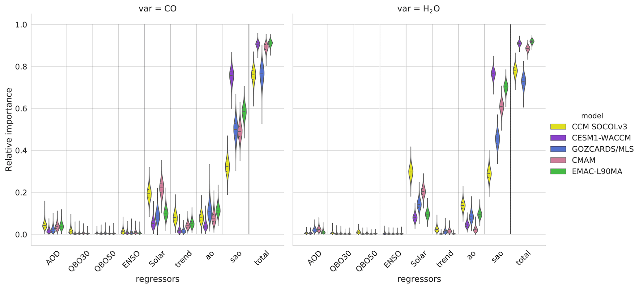
Figure 2 The full decomposition of R² from MLR of equatorial (30^∘ N–30^∘ S) CO for the period 2005–2017 and H₂O for the period 1992–2017 at 0.01 hPa in the form of violin plots. For CO observations, the Aura/MLS data are used, and for H₂O, the GOZCARDS composite are used. Distributions were calculated from 10 000 bootstrapped samples using the LMG measurements. Horizontal dashed lines represent quartiles of the distributions. Note that to quantify relative importance of the annual (AO) and semiannual (SAO) oscillations, we do not use deseasonalized time series.

4 Results

4.1 Simulated H₂O and CO responses to solar irradiance variability for the 1984–2017 period

Results of the MLR analysis of the H₂O time series from the four CCMs under consideration are presented in Fig. 3 for the full investigated time, 1984–2017, while comparisons with observations are shown in Fig. 5 for a restricted period.

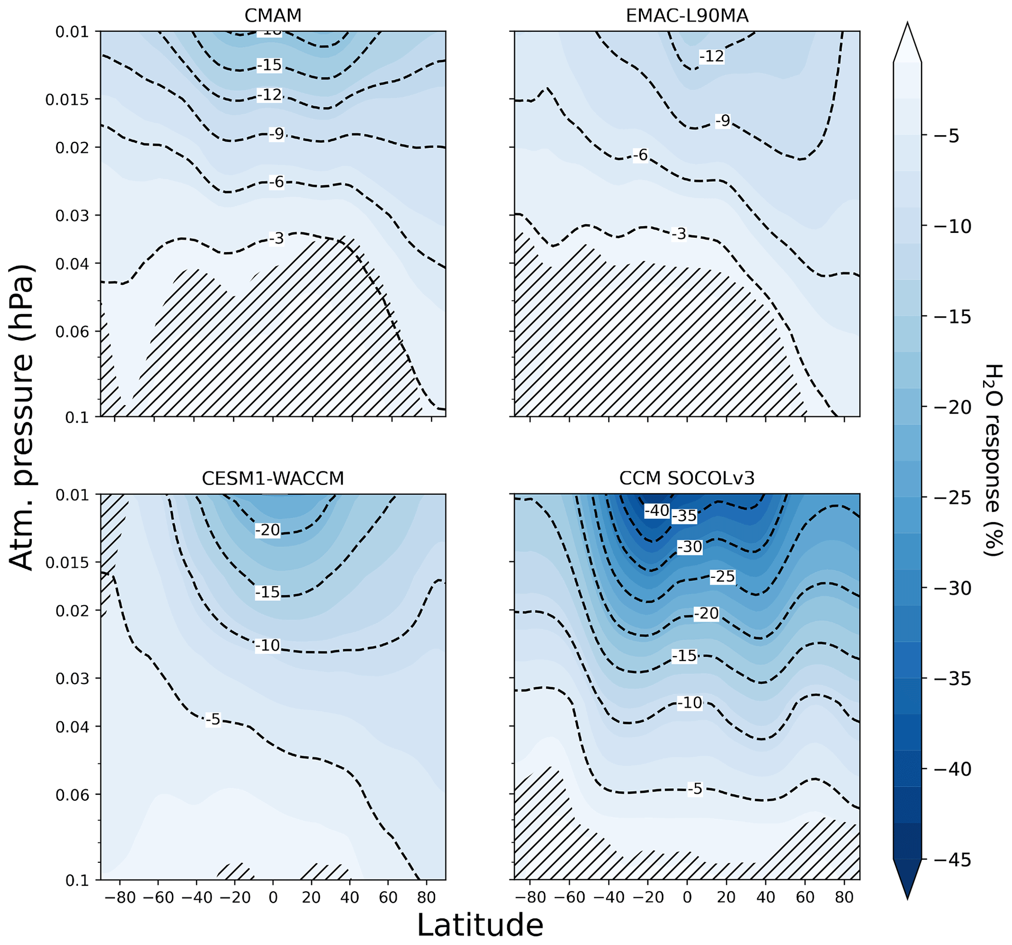
Figure 3 The relative importance of the solar signal in H₂O from CCMI-1 models (1984–2017) presented as a percentage of the mean. Model names are indicated at the top of each panel. Inclined hatches are areas with statistical significance less than 95 %.

The most pronounced effect in H₂O is seen in SOCOL and WACCM over the 30^∘ N–30^∘ S latitude band, which appears in the most sunlit region. The effect in SOCOL exceeds those from all other models with up to a 45 % H₂O response to solar irradiance variability. Such a large relative response in SOCOL can be explained by the low background water vapor mixing ratio (see Fig. 1), by a wider nudging region, or by the photolysis by Ly-α implemented in the model that is too intense. The H₂O responses simulated with CMAM and EMAC are smaller and do not exceed 20 %. The maximum of the response is slightly shifted towards the north in the CMAM, EMAC, and WACCM models, as well as the second maximum in SOCOL, which may be connected to an enhanced residual circulation modulated by the solar cycle (Cullens et al., 2016). The increased downward propagation of the solar signal can also be found in the WACCM results, in which the maximum is also a bit displaced to the north along with a strengthened descending motion over the north pole. The response of H₂O to solar irradiance variability disappears below 0.1 hPa in all models because solar irradiance of the Ly-α line cannot penetrate to this depth in the atmosphere and the influence of the Schumann–Runge band is less substantial.

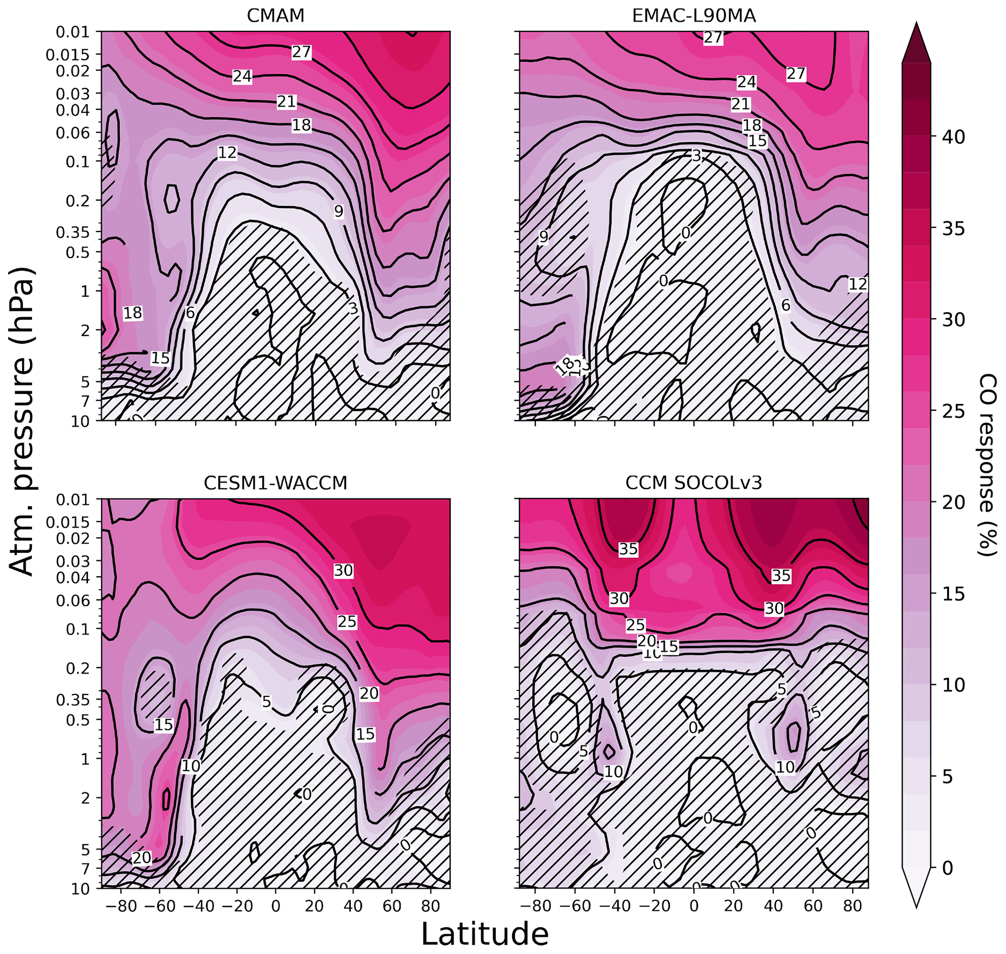
Figure 4 The relative importance of the solar signal in CO from CCMI-1 models (1984–2017) presented as a percentage of the mean. Model names are indicated at the top of each panel. Inclined hatches are areas with statistical significance less than 95 %.

Figure 4 shows the estimated CO response to solar irradiance variability in the models for the full period 1984–2017. The similar behavior in CMAM, EMAC, and WACCM suggests a descent of air enriched in CO and a large correlation with solar irradiance over the high latitudes. The penetration is deeper over the Southern Hemisphere where a stronger southern polar vortex provides more intensive downward motion and stronger isolation from the middle latitudes. A stronger meridional transport induced by enhanced atmospheric wave breaking appears to suggest a maximum CO response over middle and high latitudes in the northern upper mesosphere (Cullens et al., 2016; Lee et al., 2018). In contrast, SOCOL generates three maxima of CO (40^∘ S, 40^∘ N, and 80–90^∘ N) in the upper mesosphere between 0.01–0.1 hPa, which are not seen in the other models. Below we will see that this feature depends on the exact period chosen for comparison (see Fig. 7 below). SOCOL also shows two regions at southern and northern midlatitudes with a stronger response and statistical significance above 95 %. Again, the exact appearance of this feature depends on the exact years chosen for averaging (see Fig. 7 below). In SOCOL, a sharp boundary in the CO response is seen between 0.1 and 0.2 hPa due to the lower lifetime of CO there (the OH concentration is higher), which is too short to allow mesospheric CO to be transported down. This effect can be found in the other models as well but only in the 40^∘ S–40^∘ N latitude band. The shape of the solar signal in CO is characterized by a much deeper propagation over the middle and high latitudes, and it substantially differs from the solar signal in H₂O, which is mostly confined to the area above 0.1 hPa that is exposed to solar UV in the Ly-α line (dissociating H₂O according to Reaction R1). The reason for the difference in patterns of H₂O and CO could be a longer chemical lifetime of CO produced by Ly-α in the mesosphere over middle and high latitudes that allows for transport down through atmospheric circulation.

4.2 Simulated and observed H₂O and CO responses to solar irradiance variability

To evaluate the model performance, the simulated solar signals in H₂O and CO are compared with satellite measurements. As the observations are not available for the full time period described in the previous sections, we repeated the MLR calculations using the GOZCARDS merged H₂O time series for the 1992–2017 period and using the MLS CO time series for the 2005–2017 period. The solar signals in H₂O extracted from the slightly shorter period are illustrated in Fig. 5. For none of the models did the simulated results depend strongly on the period. The solar signal in H₂O extracted from the satellite data does not show a strong equatorial response in H₂O, as is visible in most of the model results. Instead, more pronounced effects are shifted to midlatitude zones where strong downwelling propagates the solar cycle signal to lower levels. The effects are very similar to those presented by Remsberg et al. (2018), who also obtained maximum responses shifted to the middle latitudes. The reason for such a pattern in UARS/HALOE could be related to the sampling issue over the low-tropical region. The same but with a less pronounced shape appears in the SOCOL results. In this case, the southern maximum is shifted to approximately 20^∘S and the northern maximum is shifted to high latitudes in the Northern Hemisphere. Nevertheless, in terms of percentage, WACCM, CMAM, and EMAC H₂O results are closest to the observations over the tropical zone. However, over the middle latitudes, only SOCOL shows a slight poleward shift of the maximum H₂O response, which is similar to but not quite the same as in the observations, possibly resulting from the full-atmosphere nudging applied in SOCOL.

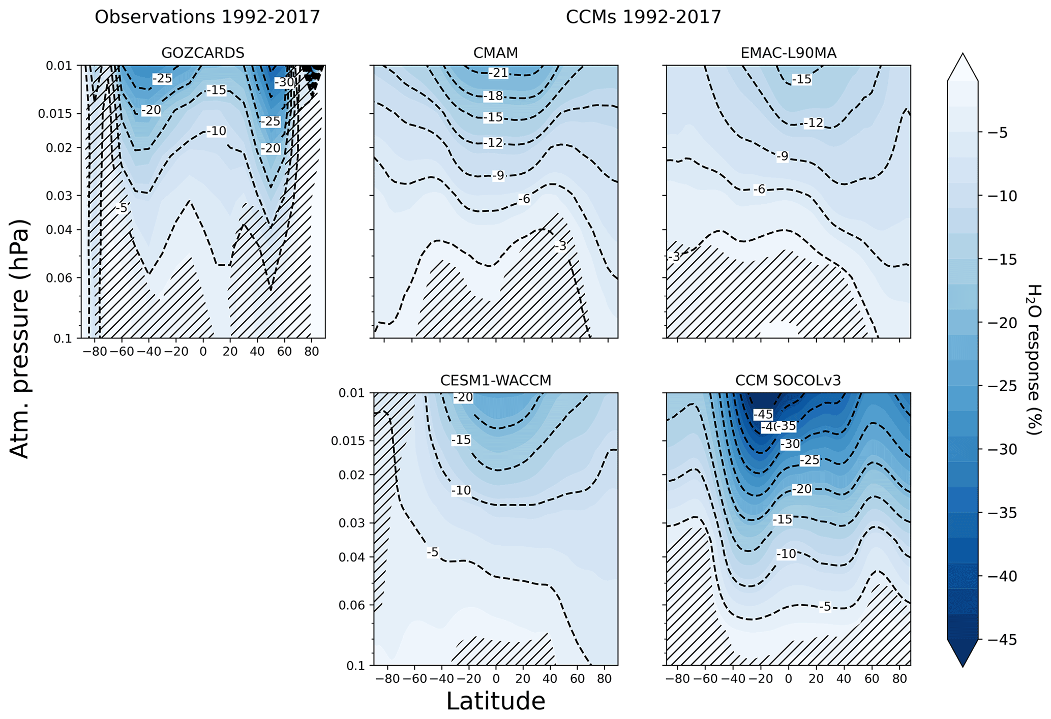
Figure 5 The relative importance of the solar signal in H₂O from CCMI-1 models and observations collected by GOZCARDS for the period 1992–2017 presented as a percentage of the mean. Model and observation names are indicated at the top of each panel. Inclined hatches are areas with statistical significance less than 95 %.

Because the latitudinal distribution can be related to the peculiarities of the satellite observations such as gaps and measurement inaccuracies, the tropical averaged plot could be more instructive for the evaluation of the model performance. Figure 6 shows the tropical response in H₂O as a percentage of the mean and the change in mixing ratio (in ppmv) averaged over 30^∘ S–30^∘ N. The effect of solar irradiance variability is largest in the tropics. Moreover, the H₂O response is less sensitive to thermospheric processes since there is no downwelling over the tropics. To make a better comparison of model results and observations, we present them not only as a ratio to the mean but also as absolute values of solar regression coefficients since the background water vapor concentrations in the considered datasets are different.

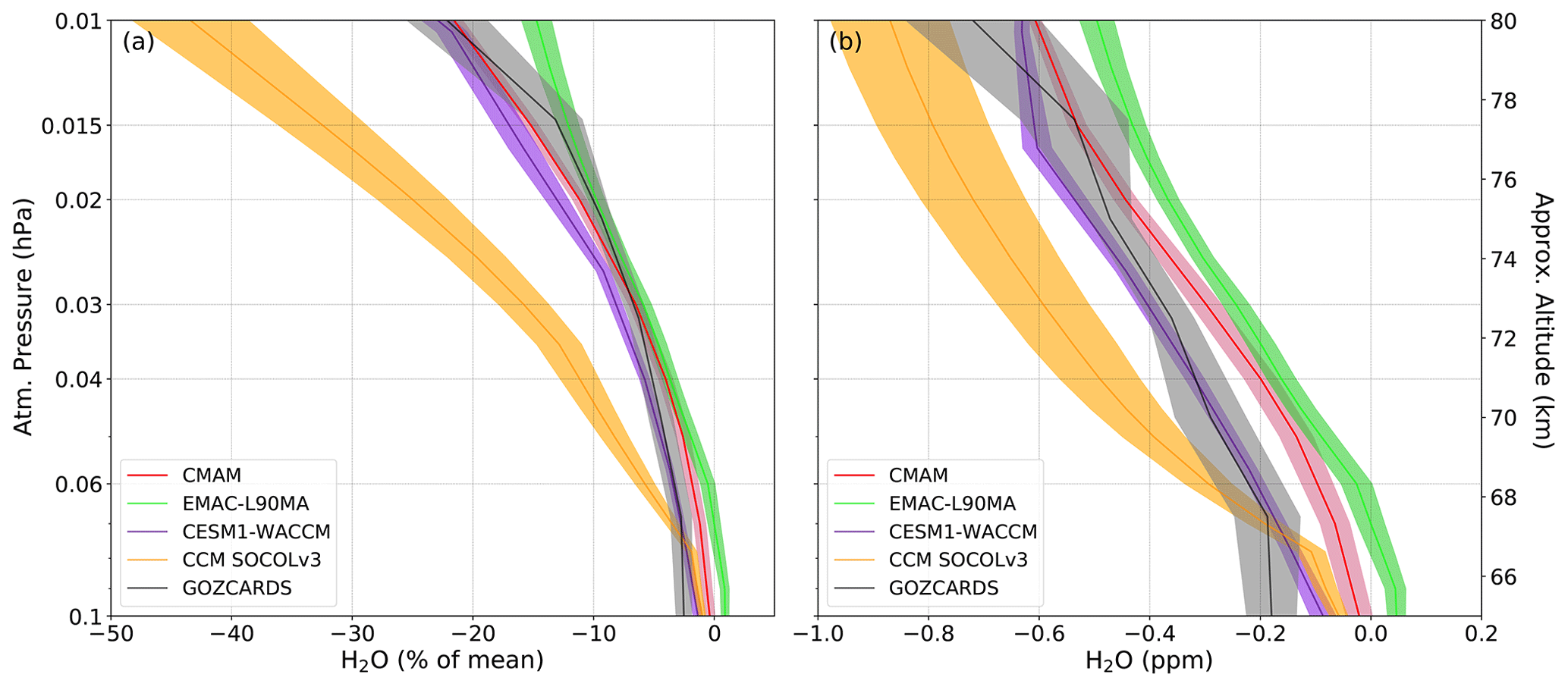
Figure 6 Vertical profiles of solar irradiance response in H₂O from CCMI-1 models and GOZCARDS observational composite for 1992–2017 at tropical latitudes (30^∘ N–30^∘ S). (a) The relative importance of the solar signal in H₂O presented as a percentage of the mean. (b) H₂O regression coefficient at the solar proxy (β) in mixing ratio (ppmv). Shadings indicate the standard deviation.

In the tropics, the observations show a steady increase in H₂O sensitivity to the solar irradiance from 0.1 to 0.01 hPa, where it reaches the maximum for both relative (23 %) and absolute (0.75 ppmv) values. Our results agree rather well with the results presented by Remsberg et al. (2018) and Nath et al. (2018). The simulated relative sensitivity values agree well with the observations. However, the SOCOL model shows a much stronger (up to 43 %) water vapor sensitivity to solar irradiance (compared with the observed 23 %). EMAC results slightly underestimate the observed values, while WACCM and CMAM show a slightly larger sensitivity. Almost the same pattern is visible for absolute sensitivity values. CMAM and WACCM show the best agreement, while SOCOL and EMAC sensitivities are too strong or too weak, respectively. In EMAC, the relative values of the solar signal in H₂O over the tropics agreed well with observations between 0.03 and 0.015 hPa, but the deviation with the solar signal in observations becomes noticeable above for which EMAC underestimates observations. For absolute values, EMAC underestimates the solar signal in H₂O for the whole presented area. Contrary to EMAC, SOCOL overestimates the solar signal in H₂O similarly for both relative and absolute values after about 0.05 hPa but underestimates it below 0.03 hPa. In WACCM, the solar signal in H₂O is mostly located within the observational uncertainty, but for relative signal, WACCM shows the pronounced deviation from observations within 0.04 and 0.013 hPa. For 0.01 hPa, WACCM and CMAM correspond well with observations in both relative and absolute values of the solar signal, although they show an underestimation in absolute value within the observational uncertainty. In the case of absolute values, CMAM agrees well with observations above and underestimates them below 0.02 hPa, but in the relative meaning, CMAM H₂O underestimates the observed solar signal below 0.04 hPa and shows an overestimation between 0.25 and 0.015 hPa, respectively.

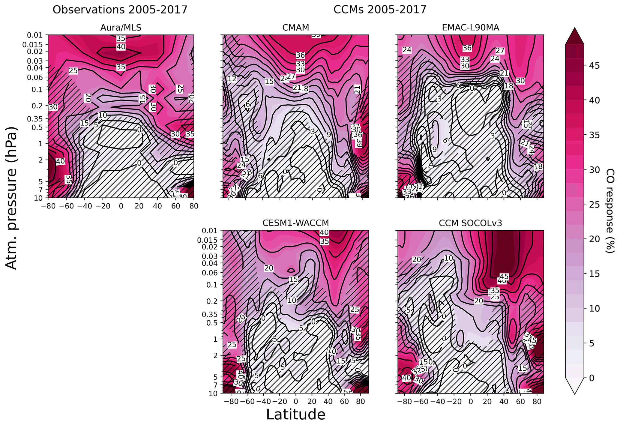
Figure 7 The relative importance of the solar signal in CO from CCMI-1 models and Aura/MLS for the 2005–2017 period presented as a percentage of the mean. Model and observation names are indicated at the top of each panel. Inclined hatches are areas with statistical significance less than 95 %.

The solar signals in CO extracted from the REF-C1SD simulations and observed by MLS data for the 2005–2017 period are illustrated in Fig. 7. In contrast to the H₂O case, the influence of the time interval is substantial. The comparison of the results from Figs. 4 and 7 reveals that the southern mesospheric maximum of the CO response to solar irradiance variability in SOCOL disappeared, while the northern one became more pronounced. The downward propagation in SOCOL is also intensified, and a large and statistically significant solar signal is visible in the upper and middle stratosphere. In CMAM and EMAC, the maximum mesospheric response is shifted from the northern midlatitudes to the equatorial area. There are two peaks of the signal in EMAC: the stronger one is over the Equator, but the second one is shifted in a similar way to SOCOL and WACCM, showing a maximum at the same pressure levels (from 0.01 hPa to the bottom of the mesosphere) and placed at the same latitude, but both are less intensive than in SOCOL. The downward propagation is visible only over the high northern latitudes in CMAM and almost disappears in EMAC. The shape of the solar signal simulated with WACCM does not change the location; it has a stronger maximum over the middle latitudes, and downward propagation is only marginally significant. This can be explained either by the shortening of the period that emphasizes some unexplored change or by different circulation patterns during the 2005–2017 period. The Aura/MLS data show a maximum in the equatorial middle mesosphere and middle stratosphere over the high southern and northern latitudes. In the mesosphere, Aura/MLS data are in a better agreement with CMAM and EMAC, while below 0.1 hPa, all models equally resemble Aura/MLS observations. Some similarity of the stratospheric response in all considered models and MLS probably results from the applied nudging, and therefore it is dynamically induced, in contrast to the mesosphere where the dynamic is only partly nudged, and the models differ substantially.

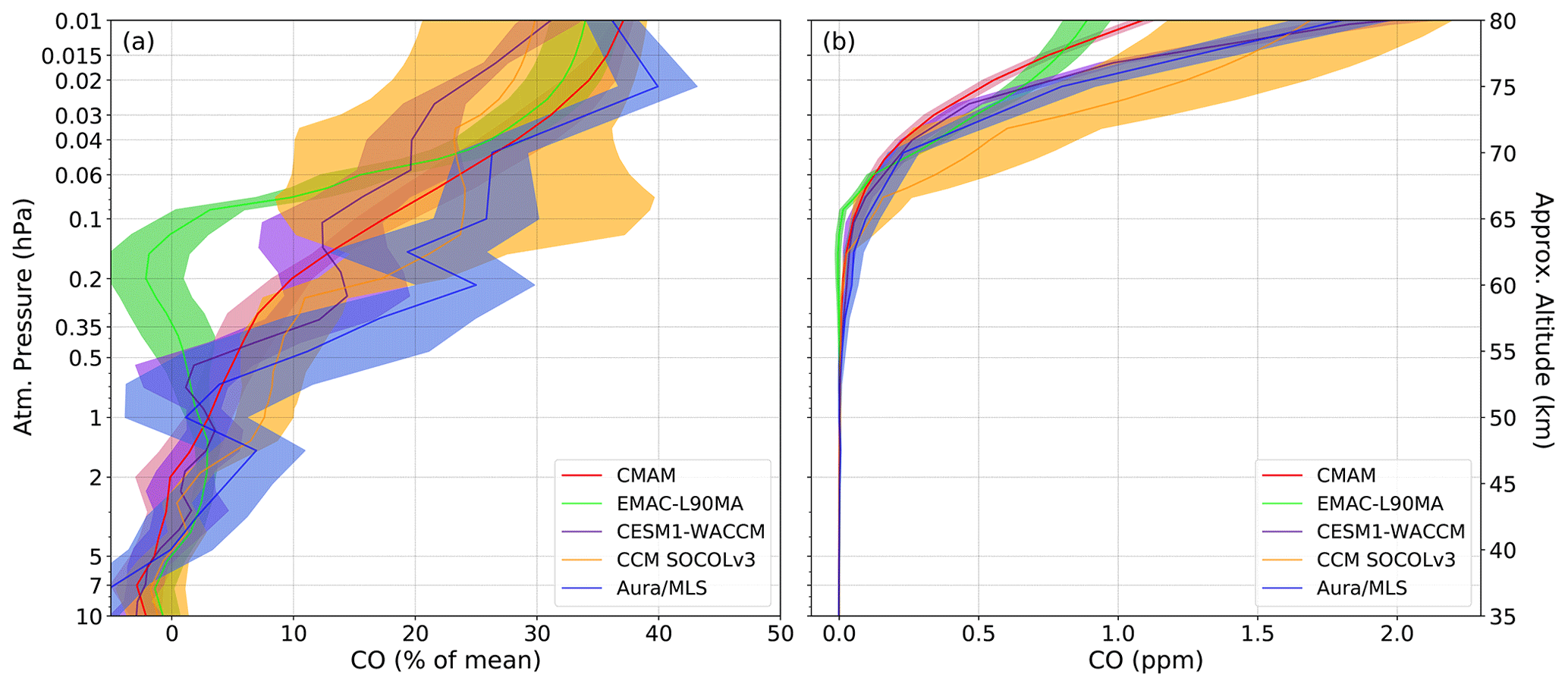
Figure 8 Vertical profiles of solar irradiance response in CO from CCMI-1 models and Aura/MLS observations for 2005–2017 at tropical latitudes (30^∘ N–30^∘ S). (a) The relative importance of the solar signal in CO presented as a percentage of the mean. (b) CO regression coefficient at the solar proxy (β) in mixing ratio (ppmv). Shadings indicate the standard deviation.

Figure 8 shows the tropical response in CO as relative change (in the percentage of the mean) and the mixing ratio (in ppmv) averaged over 30^∘ N–30^∘ S. The relative CO sensitivity to the solar irradiance variability averaged over the tropical area from the Aura/MLS data shows a positive correlation from 10 to 0.01 hPa with a magnitude of up to 40 % in the mesopause. The simulated sensitivity is within the uncertainty range of the observations for all models except EMAC between 0.35 and 0.06 hPa and except WACCM, which shows an underestimation between 0.3 and 0.01 hPa in the case of relative change. The observed absolute sensitivity in the tropical area reaches almost 2 ppmv at the mesopause and is better reproduced by SOCOL and WACCM.

5 Discussion

The comparison of absolute values (mixing ratio) of the solar signal in H₂O from models and merged UARS/HALOE and Aura/MLS (GOZCARDS) observations with previous studies reveals higher values in our study for almost all datasets. Comparing the tropical profile plot of H₂O with one from Nath et al. (2018) over the same tropical region (30^∘ N–30^∘ S), it is seen that only EMAC shows a similar magnitude to the solar signal of −0.56 ppm in H₂O from Nath et al. (2018), while all other profiles show stronger responses, including GOZCARDS, which shows −0.73 ppm at 0.01 hPa. However, Nath et al. (2018) used only Ly-α as a solar forcing, yet in the mesosphere, other wavelengths contribute significantly to H₂O photolysis and the solar signal in H₂O. The latitude-height distribution of the solar signal in H₂O from GOZCARDS and its magnitudes are in good agreement with Fig. 11 of Remsberg et al. (2018), showing similar mesospheric maxima of about 35 % over 50–60^∘ N and a minor maximum of about 25 % around 40^∘ S. A comparison with Remsberg et al. (2018) also showed similar features revealed by the MLR setup in our study. Our MLR analysis of Aura/MLS CO shows a weak solar signal of about 40 % in the mesospheric CO over the tropics compared to the solar signal in CO of 68 % from Lee et al. (2018). Also, our results show a better representation of the CO solar signal in WACCM for the period 2005–2017 in comparison with the one from Lee et al. (2018). Our results suggest that there is no dominating thermospheric influence of solar irradiance on CO as stated by Lee et al. (2018) because the signal in SOCOL CO shows reasonable results compared to WACCM CO and Aura/MLS observations. However, as mentioned above, in SOCOL the absence of a thermospheric source of CO could be compensated for by the overproduction of CO in the upper mesosphere.

However, our MLR analysis revealed a peculiar shift of the solar signal in SOCOL and WACCM, as well as a secondary peak in the same place in EMAC CO for the same period as for Aura/MLS. The nature of this probably reflects the peculiarities of the model dynamics in the Northern Hemisphere, which are in some way changed in SOCOL, WACCM, and EMAC during 2005–2017 compared to the longer 1984–2017 period. For the longer period, all models show a similar stronger signal being shifted northward and downward, and only in SOCOL does the solar signal in CO not reach levels below 0.02 hPa. Among the reasons we suggest, we categorize variations on decadal timescales that may have been attributed as the solar signal, such as global warming, accelerated Brewer–Dobson circulation (BDC), or even changes through sudden stratospheric warmings that facilitate a downward transport of air from the mesosphere. Also, as mentioned above, in SOCOL, the nudging is applied for the whole model atmosphere (1000–0.01 hPa), which could make the representation of a dynamical effect on the solar signal more reliable. The period could also play a role as the 2005–2017 period is rather short for the MLR analysis of the solar signal since this period is equal to the duration of only one solar cycle. It is important to mention that the signal in Aura/MLS does not show this shift, which makes it more difficult to understand its nature. The latitude-height distributions of the solar signal in H₂O and CO from CMAM, SOCOL, EMAC, and WACCM for different periods show that the patterns are very different. The impact of the period on our results should not be related to the aliasing of regressors, as reported in previous studies (Chiodo et al., 2014; Kuchar et al., 2017), because of the absence of any major volcanic eruptions after 2005.

Our analysis revealed deviations in simulation results from observations showing the weakness of current models in the representation of the solar signal. We hypothesize that the major problem is the model dynamics; this issue can be addressed by the application of more accurate dynamics and transport routines in models. Also, the MLR analysis revealed some inconsistencies in the solar signal presented in both absolute and relative changes compared to observations. For example, SOCOL shows a higher tropical solar signal in H₂O compared to GOZCARDS (Fig. 6), but H₂O time series (Fig. 1) show lower absolute values by about 2 ppm compared to observations.

One possible reason for the underestimation of H₂O in SOCOL is that only the H₂O + hν→ H+OH photolysis reaction is considered. It is known that H₂ + O products are also possible with about a 10 % quantum yield, although the much longer lifetime of H₂ should rather lead to a less intensive recombination of the products and even smaller H₂O concentration.

However, in the case of CO, SOCOL shows reasonably good absolute values and solar signals in both presented forms compared to the Aura/MLS CO in Fig. 8. In the case of EMAC, a weaker solar signal in H₂O, despite acceptable absolute values as seen in Fig. 1, is simulated. CMAM and EMAC CO show smaller absolute values as presented in Fig. 1, and weak solar signals in CO in both absolute values and percentage of the mean view, as shown in Fig. 8. WACCM simulates a lower absolute value of H₂O and higher CO compared to the observations, showing a higher solar signal in CO and a lower solar signal in H₂O at 0.01 hPa. Our results show that the transport of CO from the thermosphere, where CO is formed by EUV/soft X-ray photodissociation of CO₂, is not of much importance; this is seen by comparing absolute values of CO and the results of our MLR analysis between SOCOL and WACCM, in which thermospheric sources of CO are included. Surely, this is fair to say only for the periods considered here and for the MLR setup used. CO₂ is photolyzed by the Schumann–Runge continuum (SRC) too, but for SOCOL and EMAC, it does not have an impact since SRC plays a role in the thermosphere that is included neither in SOCOL nor in EMAC, which both have an upper model border at 80 km.

Any impact of volcanic activity upon CO in the upper mesosphere is not likely. However, the large eruptions that occurred around solar maxima, e.g., El Chichón in 1982 and Mt. Pinatubo in 1991, could have some minor effect on the solar signal in CO due to the aliasing effects (Chiodo et al., 2014; Kuchar et al., 2017); however, this should not be a problem after 1996.

As such, these issues inspire moderate corrections to model radiation and chemical modules, but which corrections are needed strongly depends on each model, as evidenced by our MLR analysis. We assume that an in-depth comparison of these modules will be needed to find all differences between the CCM setups. What might be an option is combining the different approaches of the simulation of the solar signal in one selected model for further analyses. Moreover, using the MLR analysis (or more advanced methods of regression analysis) to check the results of simulations from this MLR analysis is needed. The comparison of these results between themselves and with available observations could help a lot to identify the potential ways for model corrections. Also, as a way to reveal problems, especially in dynamics, the comparison of the solar signal from observations can be undertaken with not only model simulations in SD mode but also with free-running model simulations.

6 Summary

Using an MLR model, this work extracted and investigated the solar signal in the time series of the monthly averaged mixing ratio of H₂O and CO from CMAM, EMAC-L90MA, SOCOLv3, and CESM1-WACCM 3.5 REF-C1SD model simulations, as well as from UARS/HALOE and Aura/MLS measurements. The solar signal was obtained for three periods: for the 1984–2017 period to compare models between themselves, for the 1992–2017 period to compare the solar signal in H₂O from models against one from the merged UARS/HALOE and Aura/MLS (GOZCARDS) observations, and for 2005–2017 to compare the solar signal in CO from models against one from Aura/MLS. As expected, the results of our analysis show that the intensity of the signal increases upward throughout the mesosphere with a maximum at 0.01 hPa in model data and observations of H₂O and CO. However, as our analysis is limited to 0.01 hPa, the actual maximum could be higher. Thus, the variability in H₂O and CO in the mesosphere is strongly determined by the solar irradiance variability over the 11-year solar cycle with a decrease in H₂O and an increase in CO at the solar maximum, and vice versa during the solar minimum. Also, our results suggest that atmospheric transport is important for the latitudinal distribution of the considered species with a high sensitivity to solar irradiance variability. The comparison of the latitude-pressure distribution of the solar signal in H₂O for the 1992–2017 period between models and observations shows that the SOCOL model demonstrates a good agreement with the signal of the GOZCARDS observations yet with different signal strength. In the case of CO for 2005–2017, the better representation is given by the CMAM model since WACCM and SOCOL show an unexpected shift in the signal to the north. The solar signal in EMAC CO is close to Aura/MLS but has a second peak in the same latitude range as WACCM and SOCOL. The line plots over the tropics in Figs. 6 and 8, both in absolute and relative terms, show similar model results compared to observations in CMAM and WACCM H₂O, as well as in SOCOL and WACCM CO.

Overall, our analysis of the solar signal in H₂O and CO shows that the solar signal response in the tropics is confined to the mesosphere as we analyzed the solar signal up to 80 km. The H₂O and CO solar signals over the tropics decay with decreasing altitude and become negligible close to the stratopause in all considered datasets. Besides 10 % of the variance attributed to the solar signal variability, the semiannual oscillation dominates the tropical mesosphere.

To sum up, our study demonstrates how state-of-the-art models represent solar signal responses but also what the weak points of model simulations are. The intercomparison showed limitations in current simulations, which require a process-oriented validation involving the model teams. These findings strongly suggest continuing model intercomparison studies like those within SPARC, IGAC, and SOLARIS-HEPPA to improve the representation of the solar signal in global CCMs.