the Creative Commons Attribution 4.0 License.
the Creative Commons Attribution 4.0 License.
 | 10 Feb 2021
Turbulent and boundary layer characteristics during VOCALS-REx
Dillon S. Dodson
Jennifer D. Small Griswold
Boundary layer and turbulent characteristics (surface fluxes, turbulent kinetic energy – TKE, turbulent kinetic energy dissipation rate – ϵ), along with synoptic-scale changes in these properties over time, are examined using data collected from 18 research flights made with the CIRPAS Twin Otter Aircraft. Data were collected during the Variability of the American Monsoon Systems (VAMOS) Ocean–Cloud–Atmosphere–Land Study Regional Experiment (VOCALS-REx) at Point Alpha (20∘ S, 72∘ W) in October and November 2008 off the coast of South America. The average boundary layer depth is found to be 1148 m, with 28 % of the boundary layer profiles analyzed displaying decoupling. Analysis of correlation coefficients indicates that as atmospheric pressure decreases, the boundary layer height (zi) increases. As has been shown previously, the increase in zi is accompanied by a decrease in turbulence within the boundary layer. As zi increases, cooling near cloud top cannot sustain mixing over the entire depth of the boundary layer, resulting in less turbulence and boundary layer decoupling. As the latent heat flux (LHF) and sensible heat flux (SHF) increase, zi increases, along with the cloud thickness decreasing with increasing LHF. This suggests that an enhanced LHF results in enhanced entrainment, which acts to thin the cloud layer while deepening the boundary layer.
A maximum in TKE on 1 November (both overall average and largest single value measured) is due to sub-cloud precipitation acting to destabilize the sub-cloud layer while acting to stabilize the cloud layer (through evaporation occurring away from the surface, primarily confined between a normalized boundary layer height, , of 0.40 to 0.60). Enhanced moisture above cloud top from a passing synoptic system also acts to reduce cloud-top cooling, reducing the potential for mixing of the cloud layer. This is observed in both the vertical profiles of the TKE and ϵ, in which it is found that the distributions of turbulence for the sub-cloud and in-cloud layer are completely offset from one another (i.e., the range of turbulent values measured have slight or no overlap for the in-cloud and sub-cloud regions), with the TKE in the sub-cloud layer maximizing for the analysis period, while the TKE in the in-cloud layer is below the average in-cloud value for the analysis period. Measures of vertical velocity variance, TKE, and the buoyancy flux averaged over all 18 flights display a maximum near cloud middle (between normalized in-cloud height, Z*, values of 0.25 and 0.75). A total of 10 of the 18 flights display two peaks in TKE within the cloud layer, one near cloud base and another near cloud top, signifying evaporative and radiational cooling near cloud top and latent heating near cloud base. Decoupled boundary layers tend to have a maximum in turbulence in the sub-cloud layer, with only a single peak in turbulence within the cloud layer.
- Article
(6722 KB) - Full-text XML
- BibTeX
- EndNote


Stratocumulus (Sc) clouds have a significant impact on climate due to their large spatial extent, covering approximately 20 % of the Earth's surface (23 % over the ocean and 12 % over land) in terms of the annual mean (Randall et al., 1984). According to Wood (2012), the subtropical eastern oceans in particular are marked by extensive regions of Sc sheets (often referred to as semipermanent subtropical marine stratocumulus sheets). The largest and most persistent Sc deck in the world, the Peruvian Sc deck, lies off the west coast of South America (Bretherton et al., 2004), making its role in climate an essential building block to improved modeling of the overall Earth system. A better understanding of Sc decks is therefore necessary to improve our physical understanding of mechanisms controlling Sc clouds and to improve confidence in climate model sensitivity (Zhang et al., 2013), especially considering that climate models suffer from first-order uncertainties in Sc cloud representation (Noda and Satoh, 2014; Gesso et al., 2015).
It is a challenge for models to successfully simulate the Peruvian Sc deck due to the importance of subgrid scales and physical processes, which are poorly represented (Wood et al., 2011). Most models continue to struggle with the boundary layer vertical structure (Wyant et al., 2010), which is important for determining Sc cloud properties. One example, as discussed in Akinlabi et al. (2019), is that a robust estimation of the turbulent kinetic energy dissipation rate (ϵ) is needed when creating subgrid models for Lagrangian trajectory analysis of passive scalars (Poggi and Katul, 2006) or large-eddy simulation. Other vertical profiles of turbulent fluxes (liquid water, water vapor, energy) determine the mean state of the boundary layer and the resulting properties of the Sc deck (Schubert et al., 1979; Bretherton and Wyant, 1997; Ghate and Cadeddu, 2019).
Although turbulence is critical to atmospheric boundary layer, microphysical, and large-scale cloud dynamics, it is difficult to measure, with literature describing cloud-related turbulence based on in situ data being scarce (Devenish et al., 2012; Shaw, 2003). This study therefore aims to characterize turbulence throughout the vertical profile of the stratocumulus-topped marine boundary layer (STBL) over a 3-week observation period in October and November 2008 during the Variability of the American Monsoon Systems (VAMOS) Ocean–Cloud–Atmosphere–Land Study Regional Experiment (VOCALS-REx). A large in situ dataset was compiled throughout the boundary layer with the goal of improving predictions of the southeastern Pacific coupled ocean–atmosphere–land system (Wood et al., 2011). This dataset allows for a classification of turbulent properties through vertical profiles, but it also provides an opportunity to analyze how turbulence changes within the boundary layer with varying synoptic conditions.
The main objectives of this paper include a quantification of the amount of turbulence occurring within the boundary layer through the evaluation of turbulent kinetic energy (TKE), ϵ, and other turbulent flux measurements. In particular, the main goals include (1) analyzing day-to-day variability in turbulent measurements and boundary layer characteristics by relating them to synoptic changes in meteorological conditions and (2) determining average turbulent values throughout the vertical structure of the STBL by classifying the STBL based on different turbulent profiles analyzed.
There has been a plethora of publications stemming from the VOCALS-REx campaign over the last 10 years. Papers range from focusing on climatic and synoptic conditions for the VOCALS region (Toniazzo et al., 2011; Rahn and Garreaud, 2010a, b; Rutllant et al., 2013) to analyzing cloud–aerosol interactions (Jia et al., 2019; Blot et al., 2013; Painemal and Zuidema, 2013; Twohy et al., 2013), precipitation, boundary layer decoupling, and other boundary layer characteristics (Jones et al., 2011; Bretherton et al., 2010; Terai et al., 2013; Petters et al., 2013; Zheng et al., 2011), to name a few. A total of five aircraft platforms and two ship-based platforms were utilized during VOCALS-REx (Wood et al., 2011), with most publications from VOCALS-REx relying and/or focusing on aircraft observations and other data sources outside those used here (all but Zheng et al., 2011, and Jia et al., 2019, mentioned above). Results found and presented here therefore provide not only a collection of in situ turbulent measurements, but also the opportunity to relate results to other findings at additional measurement locations within the VOCALS domain. An extensive look at the turbulent characteristics of the boundary layer during VOCALS-REx does not exist (note that although Zheng et al., 2011, do give a broad analysis of boundary layer characteristics, their focus on turbulence was minimal), which is puzzling given that the Twin Otter aircraft (the data used here; see Sect. 2.1) was instrumented to make turbulence measurements.
Section 1.1 introduces typical boundary layer vertical structure and scientific background. Section 2 provides an overview of the data and methods, followed by synoptic and boundary layer characteristics during VOCALS-REx in Sect. 3. Section 4 evaluates and discusses the results. Section 5 provides concluding remarks.
1.1 Boundary layer vertical structure
The vertical structure of the boundary layer is strongly tied to the horizontal and vertical structure of Sc clouds (Lilly, 1968; Bretherton et al., 2010). The STBL is characterized by Sc cloud tops located at the base of an inversion, with subsiding air aloft, well-mixed conditions, and nearly constant conserved variables with height throughout the depth of the boundary layer (Wood, 2012). Multiple papers have analyzed typical well-mixed STBL vertical structures (i.e., Albrecht et al., 1988; Nicholls, 1984), showing a constant potential temperature and mixing ratio throughout the depth of the boundary layer up until the inversion, when the mixing ratio (potential temperature) sharply decreases (increases). Horizontal winds (both direction and velocity) are typically constant throughout the depth of the well-mixed boundary layer, with changes in both direction and strength typically present at the top of the STBL, influencing cloud-top entrainment (Mellado et al., 2014; Kopec et al., 2016; Schulz and Mellado, 2018).
Convection within the STBL is primarily driven by cooling near cloud top and not heating at the ocean surface, where cloud-top cooling is primarily from a combination of (1) longwave radiational cooling and (2) evaporational cooling from entrainment. The cloud-top cooling leads to instability and the convection of warmer, moist air at the surface (Lilly, 1968). The cloud cover is greatest when the STBL is shallow [, where zi is the inversion layer (i.e., boundary layer) height (Wood and Hartmann, 2006).
The boundary layer top is characterized by several strong gradients, including the cloud boundary (gradient in liquid water content), the entrainment zone (gradient in vorticity), which separates regions of weak and strong mixing between laminar (warmer and drier) flow above and turbulent (cooler and more moist) flow below, and the capping inversion (gradient in potential temperature). The cloud boundary typically lies in the entrainment zone (Albrecht et al., 1985; Kurowski et al., 2009; Malinowski et al., 2013), which in turn lies in the capping inversion, although these layers do not necessarily coincide (Mellado, 2017). Turbulent analysis of these layers in Jen-La Plante et al. (2016) found that turbulence (both TKE and ϵ) decreases moving from cloud top into the free atmosphere above. Through cloud-top entrainment, the STBL deepens beyond 1 km and can become decoupled. According to Bretherton and Wyant (1997), due to longwave cooling at the cloud top being unable to maintain mixing of the positively buoyant entrained air over the entire depth of the STBL, the upper (cloud-containing) layer becomes decoupled from the surface moisture supply.
The buoyancy flux (which is dependent on moisture and heat fluxes that drive buoyancy differences) can tell one a lot about the state of the STBL. Vertical energy and moisture fluxes must be linear functions of height for a boundary layer to remain well mixed, which is not the case for a cloud-containing boundary layer (Bretherton and Wyant, 1997). An increase in the buoyancy flux above cloud base is typically proportional to the upward transport of liquid water that is required to sustain the cloud against entrainment drying (i.e., continued mixing of the cloud layer is sustained by surface fluxes). Decoupling of the boundary layer (and the subsequent decrease in cloud cover) can occur when the sub-cloud buoyancy fluxes become negative, capping convection below cloud base (Albrecht et al., 1988; Ackerman et al., 2009). According to Shaw (2003), one of the main sources of TKE in clouds is evaporative cooling (due to the entrainment of dry air) and condensational heating (due to droplet condensational growth), implying that the buoyancy flux is the primary generator of TKE in the STBL (Schubert et al., 1979; Heinze et al., 2015). Given this, the buoyancy flux nearly always has a maximum in the cloud layer (Nicholls and Leighton, 1986; Bretherton and Wyant, 1997), with TKE being generated due to longwave and evaporational cooling at cloud top and condensational heating at cloud base (Moeng et al., 1992).
The main source of moisture for the STBL is supplied by the surface latent heat flux (LHF), making it an important source of buoyant TKE production (Bretherton and Wyant, 1997), with the surface sensible heat flux (SHF) typically being a much weaker source of turbulence. An enhanced LHF leads to increased moisture transport to the cloud layer and a thicker cloud, producing enhanced entrainment cooling near cloud top and more turbulence. Enhanced entrainment results in a deepening of the boundary layer, which favors decoupling (Jones et al., 2011). It is argued in Bretherton and Wyant (1997) and Lewellen et al. (1996) that the surface LHF is the most important determinant of decoupling within the STBL.
Vertical velocity variance typically displays the strongest updrafts and downdrafts in the upper half of the STBL (Hignett, 1991; Heinze et al., 2015; Mechem et al., 2012), consistent with the largest production of turbulence being contained within the cloud layer. A positive (negative) vertical velocity skewness indicates that strong narrow updrafts (downdrafts) are surrounded by larger areas of weaker downdrafts (updrafts). It has been found that negative vertical velocity skewness is typically contained within most of the cloud layer and below (Nicholls and Leighton, 1986; Nicholls, 1989; Mechem et al., 2012) for well-mixed boundary layers, whereas a decoupled boundary layer may contain positive vertical velocity skewness (de Roode and Duynkerke, 1996) due to convection being driven in the surface layer. The tendency of the vertical velocity skewness to be positive in a strongly precipitating STBL is also well known (Ackerman et al., 2009), with precipitation being a key contributor to boundary layer decoupling (Rapp, 2016; Yamaguchi et al., 2017; Feingold et al., 2015).
2.1 Data
Data were collected during the Variability of the American Monsoons (VAMOS) Ocean Cloud–Atmosphere–Land Study Regional Experiment (VOCALS-REx) from the Peruvian stratocumulus deck off the west coast of Chile and Peru during October and November 2008. VOCALS-REx used various platforms, including five aircraft and two research vessels, to accumulate an extensive dataset of the boundary layer, lower free troposphere, and cloud deck along 20∘ S from 70 to 85∘ W. Although multiple sampling platforms, locations, and mission types were deployed during the campaign (see Wood et al., 2011), data collected by the Center for Interdisciplinary Remotely-Piloted Aircraft Studies (CIRPAS) Twin Otter aircraft will be the focus of this paper, which were collected in the vicinity of 20∘ S, 72∘ W; from here on it is termed Point Alpha. The Twin Otter aircraft was operational for 19 flights from 16 October to 13 November 2008.
The Twin Otter platform is ideal for a turbulent analysis of the boundary layer due to the aircraft being instrumented to make turbulence and cloud microphysics measurements, with the same location being sampled for each flight. The Twin Otter is also a relatively slow-moving aircraft with a flight speed of roughly 55 to 60 m s−1, allowing for a higher resolution of spatial sampling compared to a faster-moving aircraft. Each of the Twin Otter flights was carried out using a stacked flight path (Wood et al., 2011), which involved using stacked legs of 50–100 km in length (horizontal flight paths) to sample various levels of the boundary layer and cloud layer, with at least one aircraft vertical sounding (vertical profile) performed for each flight during which the aircraft sampled the free upper troposphere and boundary layer in a single ascent or descent. Each flight of 5 h originated from Iquique, Chile, allowing for roughly 3 h of sampling at Point Alpha.
Of the 19 flights performed by the Twin Otter, 18 are used here due to instrumentation failure on one of the flights (5 November). Table 1 displays each of the research flights (RFs) used in this paper. All flights occurred during the day, with all but two flights (RF8 and RF17) starting around 07:00 local time and the first vertical profile flown around 08:00 local time at Point Alpha. Having each flight sample the same location at roughly the same time is critical, as turbulence typically displays diurnal patterns, with the strongest turbulent mixing occurring during the night when longwave radiational cooling dominates due to the absence of the stabilizing effect of shortwave absorption (Hignett, 1991); solar absorption is largest near cloud top due to the scattering of solar radiation, limiting absorption lower in the cloud layer (Stephens, 1978).
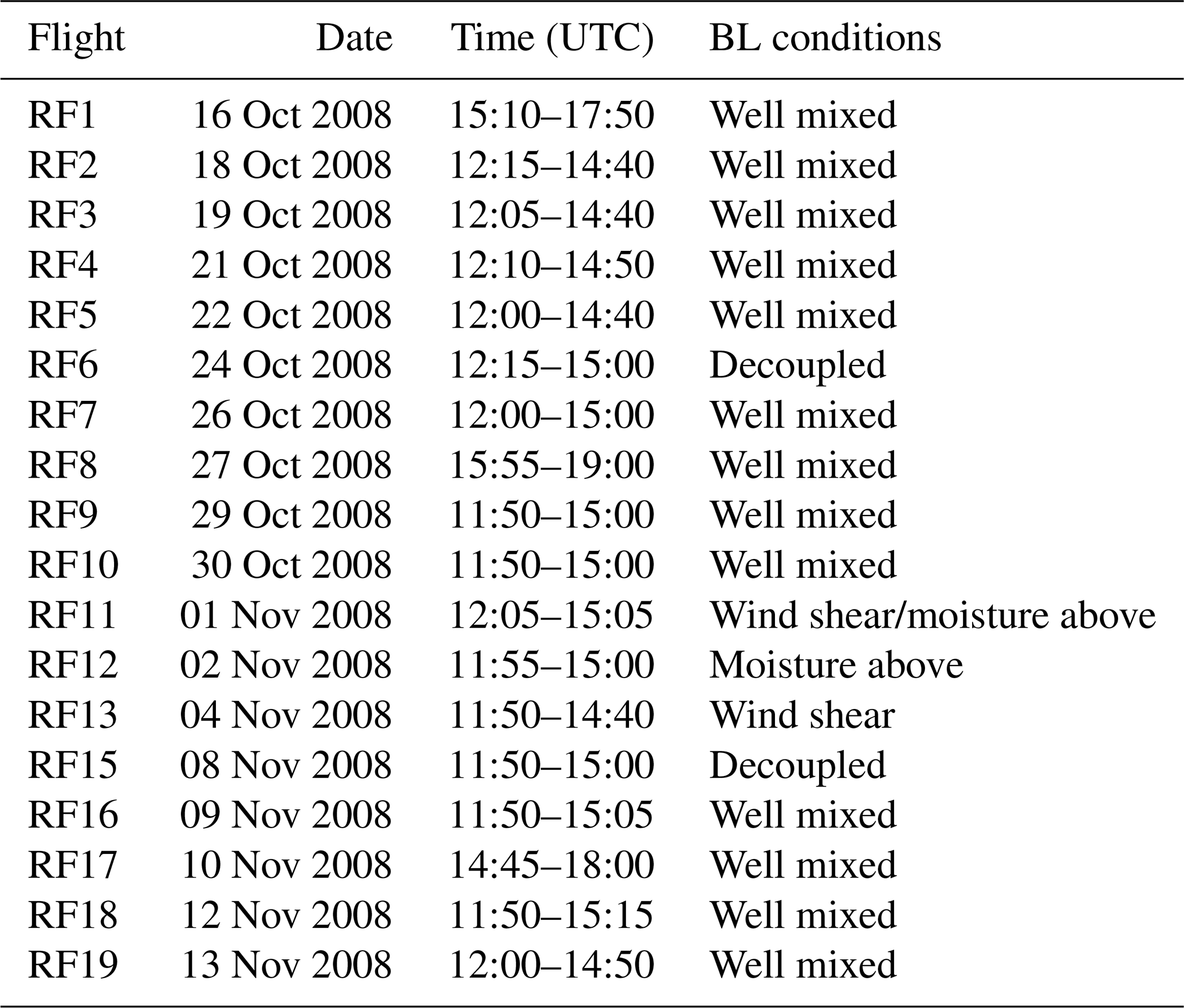
Table 1Column (1): research flight (RF) identification; column (2): the corresponding date; column (3): flight start and end times at Point Alpha. Note that local time is 04:00 UTC. Column (4): boundary layer conditions for each flight.
Meteorological variables were collected at 40 Hz (including u, v, wind velocity w, water vapor mixing ratio q, and potential temperature θ, to name a few), while most cloud and aerosol data were collected at 1 Hz. A five-port Radome wind gust probe was used with plumbing that effectively trapped liquid water, preventing any liquid water from obstructing the pressure transducer lines. There were zero failures during the campaign, with an accuracy of ±0.4 m s−1 for horizontal wind components and ±0.2 m s−1 for vertical velocity. A LI-COR 7500 gas analyzer was used for all measurements of absolute humidity and q, with an ambient air intake setup that resulted in the LI-COR source and detector window being liquid-free, even during prolonged cloud penetrations. The LI-COR accuracy is reported to be within 1 % of the actual reading. Further instrumentation information can be found in Zheng et al. (2010) and Wood et al. (2011).
To analyze the synoptic conditions over the study period, data from the National Centers for Environmental Prediction (NCEP)/National Center for Atmospheric Research (NCAR) Reanalysis Project (NNRP; Kistler et al., 2001) will be used. The data resolution of the NCEP/NCAR reanalysis data is pressure levels, available at 6 h intervals. The resolution of these data is suitable for analyzing synoptic-scale patterns but is not ideal for depicting mesoscale variability that may be present on any given day. Boundary layer height is also derived from relative humidity data from the European Centre for Medium-Range Weather Forecasts (ECMWF) Reanalysis (ERA5), which has a resolution of pressure levels and is available at an hourly interval (Hersbach et al., 2020).
2.2 Turbulent calculations
The randomness of turbulence makes deterministic description difficult, limiting descriptions to statistics and average values of turbulence, e.g., Reynolds decomposition (or averaging). Reynolds decomposition uses a mean value (over some time period, determined by low-pass filtering or applying a linear trend) and subtracts it from the actual instantaneous velocity to obtain the turbulent component (or perturbation value). Reynolds decomposition is based on the underlying assumption that the turbulence is isotropic and stationary; however, these conditions are hardly ever fulfilled for atmospheric boundary layer flows, especially when working with data spanning larger timeframes. The problem is defining how to average collected data to best represent the mean and turbulent components for the fluid flow (with shorter subsets of data having more stationary properties in general than longer subsets of data). Using the 40 Hz data, a 320-point averaging window is used here for all turbulent analysis, analogous to the methods outlined in Jen-La Plante et al. (2016). A 320-point averaging window corresponds to 8 s subsets of data, or a roughly 440 m subset of data in the horizontal spatial scale (assuming an average aircraft speed of 55 m s−1). Linear regression is then applied to each 320-point averaging window to calculate the mean and determine the perturbation values.
Applying the averaging method discussed above leads to the calculation of the fluctuations of the u, v, and w components of the velocity, along with other parameters used to measure various turbulent fluxes. Variables to be obtained include turbulent kinetic energy, which is given by
where u′, v′, and w′ are the fluctuations of the velocity components. The turbulent sensible heat, latent heat, and buoyancy fluxes will also be obtained, given by
respectively, where Cp is the specific heat of air (1005 ), Lv is the latent heat of vaporization at 20 ∘C (2.45×10⁶ J kg−1), ρ is the mean air density, and θ′, q′, and are the potential temperature, mixing ratio, and virtual potential temperature perturbations, respectively. Note that θv (given by ) is commonly used as a proxy for density when calculating the buoyancy. Humid air has a warmer θv because water vapor is less dense than dry air, while liquid water drops (if falling at terminal velocity) make the air heavier and are therefore associated with a colder θv, where ql is the liquid water mixing ratio.
Just like that of the Reynolds decomposition, the calculation of ϵ is based on the assumption that the flow is isotropic (i.e., uniform in all directions), making the measurement of ϵ challenging. In particular, classical turbulence theory in the inertial subrange from Kolmogorov (1941) is based on assumptions of local isotropy. With that said, there are multiple methods to measure ϵ, including the inertial dissipation method, structure functions, and the direct method. Siebert et al. (2006) found that both the inertial dissipation and structure function methods are useful, but the inertial dissipation method sometimes underestimates ϵ at low values due to no clear inertial subrange behavior being observed in the power spectral density, which is not the case for the structure function. The structure function method is therefore considered more robust for cases with small values of ϵ, and will be used here. Due to questions of isotropy, ϵ will be evaluated on the u, v, and w components of the wind, and an average dissipation rate will be calculated from the three components.
The calculation of ϵ comes from the analysis of the velocity fluctuations through the nth-order structure function (i.e., a statistic to analyze common variation in a time series). The structure function is given by
where l is the distance (or in the case of a temporal series, l is equivalent to t assuming constant flight speed). From Frisch (1995), ϵ using the nth-order structure function can be obtained by
where Cn is a constant of order 1. The second-order structure function (n=2) will be used here, where C2=2 for transverse velocity fluctuations, C2=2.6 for longitudinal velocity fluctuations (Chamecki and Dias, 2004), vertical fluctuations are considered transversal, and horizontal fluctuations are considered longitudinal. The structure function follows a power law within the inertial subrange and will only be used to calculate ϵ between frequencies of 0.3 and 5 Hz, neglecting the higher-frequency features attributed to interactions with the plane (i.e., vibrations due to the aircraft) and other instrumental artifacts.
Figure 1a provides the power spectral density of vertical velocity and q for three horizontal flight legs within RF3, one in cloud, one sub-cloud, and one near the surface. Note that the power spectral density follows a power-law fit (red) within the inertial subrange (as opposed to the 2/3 power-law fit of the structure function). A spike in energy can be seen at ≈10 Hz, which represents the aircraft interactions discussed previously. The power spectral density overlaid in black represents a single calculation using a 320-point averaging window. The data follow the fit well, and the inertial subrange is well resolved for the averaging window used (with the light gray envelope representing the 0.3 to 5 Hz range). A lack of significant flattening within the power spectra at higher frequencies suggests that the random noise level is low (this is more evident in the vertical velocity spectra than the q spectra).
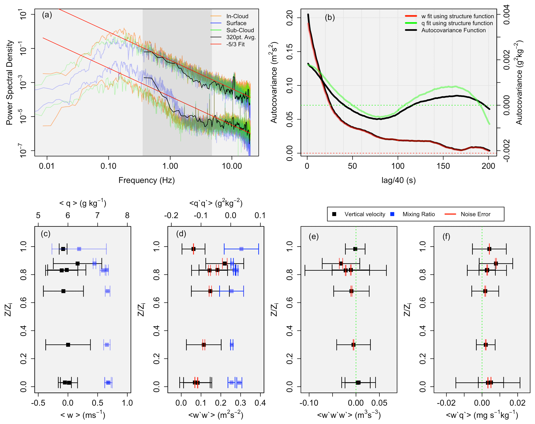
Figure 1All data presented are from RF3. (a) Power spectral density for three different horizontal flight legs, including in-cloud (orange), sub-cloud (green), and near-surface (blue) fit with a power law (red); the upper fit is vertical velocity (m2 s−1), and the lower fit is q (g2 kg−2). The overlaid black spectra represent a single spectrum using a 320-point average. The light gray envelope represents the 0.3 to 5 Hz range. (b) Autocovariance functions of vertical velocity and q (black) with the fit structure function (green for q and red for vertical velocity). (c) Leg-mean vertical velocity (black) and q (blue), wherein the error bars represent the square root of the total variance. (d) As in (c), except for the variance. Red error bars represent the noise error, while the remaining error bars represent the sampling error. (e) As in (d), except for vertical velocity skewness. (f) As in (d), except for the flux .
Analysis of the turbulence as presented here introduces two types of error: sampling and noise error. This must be analyzed to determine the statistical significance when analyzing vertical profiles, especially since error propagation into higher-order moments can be significant (McNicholas and Turner, 2014). Sampling errors were estimated using approaches derived and discussed in Lenschow et al. (1994, 2000) and will not be repeated here. Noise error must be considered, as noise within the instrumentation may be significant enough that the atmospheric component of the variance is small compared to the overall measured variance. Noise is measured using the extrapolations of the measured autocovariance functions to lag 0 by the structure function. This technique was introduced in Lenschow et al. (2000) to estimate the noise contribution from the second- to fourth-order moments. Although this technique was traditionally used to estimate lidar noise (Wulfmeyer, 1999; Wulfmeyer et al., 2010, 2016), it has also been extended to in situ observations (Turner et al., 2014).
Figure 1b provides the autocovariance function of vertical velocity and q for a sub-cloud fight leg in RF3 (black). The fit using the structure function is provided in red (vertical velocity) and green (q). The structure function at lag zero provides the mean variance, while the difference between the autocovariance and structure function at lag zero provides the system noise variance at the corresponding temporal resolution. It is clear that the atmospheric variance and noise can be separated. For example, from panel (b), looking at the vertical velocity data, m2 s−2 and the noise variance m2 s−2. This results in a noise standard deviation of δw=0.12 m s−1.
Extending this analysis to determine the error propagation within higher-order moments, error bars for vertical velocity () and q variance (), vertical velocity skewness (), and the kinematic moisture flux () can be found in panels (d) through (f), respectively, with noise error bars in red and sampling error bars in black. The noise error is negligible compared to the sampling error, in agreement with results from Turner et al. (2014). Note that some data points do not have noise error bars associated with them. This is due to the fact that the noise was so small, the error bars were negligible. The various vertical profiles displayed show that the sampling errors result in a lack of statistical significance between flight legs of different altitudes.
Equations used to determine the noise in the higher-order moments from Wulfmeyer et al. (2016) are
where N is the number of data points. Using Eq. (7), the absolute error for the vertical velocity variance is found to be 0.00068 m2 s−2 and the relative error is 0.35 % (the relative error for the q variance is 1.9 %). Both errors are very reasonable, and demonstrate the low noise of the instrumentation.
3.1 Synoptic variability at Point Alpha
The southeastern Pacific Ocean is found on the eastern edge of the South Pacific semipermanent subtropical anticyclone, characterized by large-scale upper-tropospheric subsidence that leads to a strong temperature inversion with a well-mixed boundary layer below. The surface pressure is therefore controlled in part by the location of the South Pacific subtropical anticyclone. This anticyclone is routinely interrupted (especially between fall and spring) by periods of relatively low pressure, which are associated with localized troughing or the passage of midlatitude cyclones to the south. Several papers (Toniazzo et al., 2011; Rahn and Garreaud, 2010a) have analyzed the synoptic characteristics during VOCALS-REx. These papers, however, tend to focus on the VOCALS-REx region as a whole and not specifically on Point Alpha, which is done here.
Spatial maps of the mean sea level pressure and 700 hPa geopotential height (not shown here; see Zheng et al., 2011, or Toniazzo et al. (2011), for a visual) display the anticyclone near its climatological position of 30∘ S, 100∘ W. While enhanced storm tracks were primarily contained within the midlatitudes, the standard deviation in the 700 hPa geopotential height map displays midlatitude troughing that extended between Point Alpha and the subtropical high (Zheng et al., 2011), suggesting that meteorological conditions at Point Alpha were influenced by both midlatitude synoptic systems and the subtropical anticyclone.
Synoptic variability at Point Alpha is summarized in Fig. 2 by time series of geopotential height at 500 and 700 hPa. Higher geopotential heights are associated with ridging aloft, while decreases in geopotential heights are associated with synoptic disturbances or troughs. The 500 hPa geopotential height varied between 5840 and 5900 m, with a decrease of 27 m between 16 October and 13 November. Figure 2 also displays enhanced synoptic-scale variation during October, with several disturbances affecting Point Alpha. The 500 and 700 hPa geopotential heights alternate between areas of high and low height through 2 November. After 2 November, the 500 hPa geopotential height is more consistent, with height increasing over Point Alpha until 10 November, at which point the height begins to decrease.
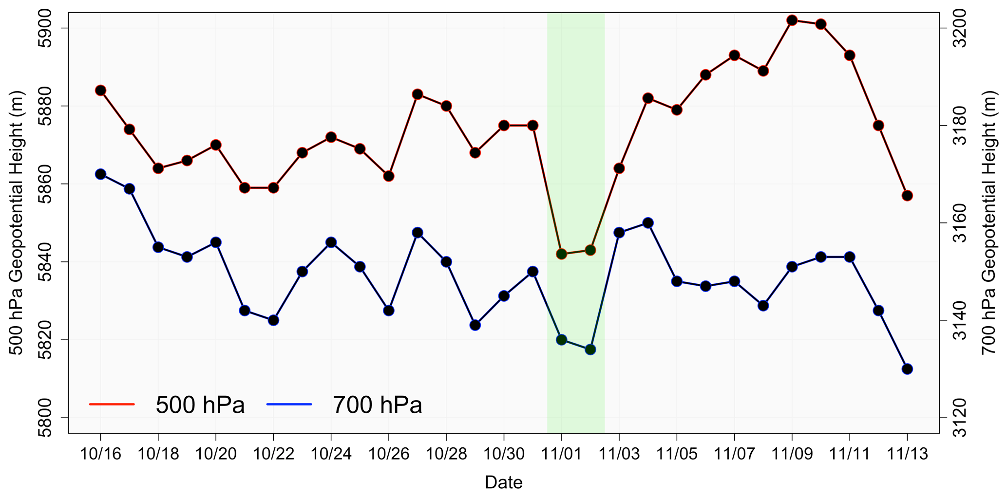
Figure 2The 500 hPa (red) and 700 hPa (blue) geopotential height from the NCEP/NCAR reanalysis data.
Besides minor disturbances in October, there are two main disturbances that stand out. The first disturbance occurs on 1 and 2 November (green shading in Fig. 2), when both the 500 and 700 hPa heights have a minimum (5842 and 3134 m, respectively) due to the influence of a synoptic system. The second disturbance was the formation of a coastal low, which can be seen by decreasing geopotential heights on and after 10 November. This coastal low reached a minimum (the coastal low was strongest) after the analysis period on 15 November (Rahn and Garreaud, 2010a). The ridging that formed after 2 November leads to the formation of the coastal low through the warming of the lower and middle troposphere (Garreaud and Rutllant, 2003).
The 700 hPa geopotential height map (not shown here) displays a midlatitude trough developing and extending past Point Alpha from 29 October through 3 November. A deep midlatitude trough forms off the west coast of South America by 30 October, extending past 15∘ S. The trough axis begins to move over Point Alpha by 31 October, with the main impacts of the trough on Point Alpha (in terms of lowest geopotential height) being observed on 1 and 2 November. The 500 hPa geopotential height map (not shown here) shows the ridge axis directly over Point Alpha on 1 November.
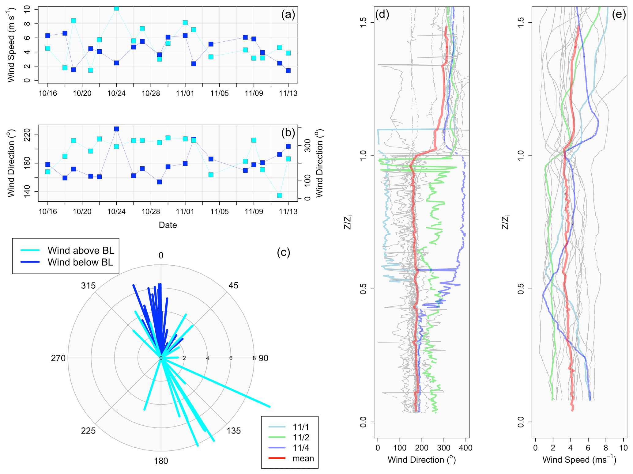
Figure 3(a) Wind speed (m s−1) at the surface collected during 30 m horizontal flight legs (dark blue) and above the inversion collected during horizontal flight legs above the boundary layer (light blue). (b) As in (a), except for wind direction (degree). (c) Vectors showing wind direction from (b). (d) Vertical profiles (collected during aircraft soundings) of wind direction for each flight day plotted vs. normalized boundary layer height; 1 and 4 November are displayed in light blue and dark blue, respectively, while 2 November is in green, and the mean wind direction is represented by red. (e) As in (d), except for wind speed (m s−1).
Figure 3a–c show atmospheric wind direction and velocity using data collected from horizontal flight legs. Panels (d) and (e) display wind direction and speed, respectively, using data collected from aircraft vertical soundings. Atmospheric winds near the surface (measured during 30 m horizontal flight legs) at Point Alpha were mostly southerly (150 to 230∘) with a mean of 179∘. Strong wind shear was present near the inversion, with winds above the marine boundary layer (measured during horizontal flight legs above the inversion) having a mostly northwesterly component (mean of 276∘) while having more variability in direction than the boundary layer. Although on most flight days the wind speed and direction were constant with height throughout the depth of the boundary layer (see panels d and e), on 1 and 4 November (light blue and dark blue lines, respectively) the wind direction shifted sharply within the boundary layer from southerly to northeasterly, along with varying wind speed. On 2 November (green line), the wind direction had a westerly component (214∘). Shear within the boundary layer is not common. Zheng et al. (2011) suggest that this shear is linked to coastal processes such as the propagation of the upsidence wave. It should also be noted, however, that the wind shear within the boundary layer is present on the same day (1 November) that the trough axis is located over Point Alpha. On the following day, the surface winds experienced their second-most westerly component (24 October has the most westerly component). According to Rahn and Garreaud (2010a), as troughs approach the coast of South America, southeast winds are typically replaced by southwest winds. Between 29 October and 2 November, wind direction within the boundary layer shows the most variation, gradually shifting from 153∘ (most easterly component measured) to 214∘ (second most westerly component). While the trough approaches the coast of Chile, southeast winds are replaced by southwest winds, as is typical of synoptic-scale disturbances in the region (Rahn and Garreaud, 2010a). Note that the most westerly component of the boundary layer wind measured on 24 October coincides with a dip in the geopotential height (with winds quickly shifting back to easterly), suggesting a weak disturbance on 24 October.
3.2 Boundary layer characteristics
Boundary layer height is perhaps the most important feature of the marine boundary layer (MBL), with zi being one of the main metrics for boundary layer characteristics such as decoupling and cloud cover (Albrecht et al., 1995). Figure 4 shows the thickness of the Sc cloud layer, the thickness of the inversion layer, and subsequently the MBL height for each flight. The expected lifted condensation level (LCL) for a well-mixed boundary layer is also provided, using , where Td is dew point temperature. zi is also provided from extrapolating relative humidity data from the ECMWF reanalysis (Engeln and Teixeira, 2013). The cloud layer was identified using a liquid water content (LWC) greater than or equal to 0.01 g m−3, while the inversion layer was identified by the region of greatest change in q (absolute change ≥0.10 g kg−1 per 1 Hz measurement) and θ (absolute change ≥0.20 K per 1 Hz measurement) within the vertical profiles. This results in the bottom of the inversion layer characterized by the profiles beginning to lose boundary layer features, while the top of the inversion layer has lost all boundary layer features.

Figure 4The range of the cloud (gray) and inversion (blue) layer as a function of altitude for each RF. The top of each gray profile represents cloud top and zi. The bottom of each gray profile represents cloud base. Cloud thickness (represented as a single value) is represented by each red dot (right y axis). The LCL and ECMWF zi are shown as the black star and green x, respectively.
The average zi was 1148 m (see Table 2 for boundary layer characteristics), with the average cloud layer and inversion thickness being 229 and 55 m, respectively. Figure 4 shows that zi varied between 996 and 1450 m, with mostly gradual changes in height from flight day to flight day (note that the mean difference between zi and ECMWF zi was 44±24 m). The average change in zi (in regards to the in situ data) was 88 m d−1 with five occurrences of a rate of change above 100 m d−1. For cloud thickness, the most significant changes took place after 27 October, peaking on 1 and 2 November with thicknesses of 382 and 472 m, respectively. Although the time series of cloud droplet number concentration (Nd) is not shown here, we observed a notable dip to a minimum on 1 November of 81 cm−3 (the average is 280 cm−3), corresponding to a minimum in both boundary layer cloud condensation nuclei (CCN) and aerosol number concentration (Na), along with a maximum in average drop size.
Table 2Mean, standard deviation, and range of values for select variables over the 18 flights analyzed, with standard deviation values in parenthesis.
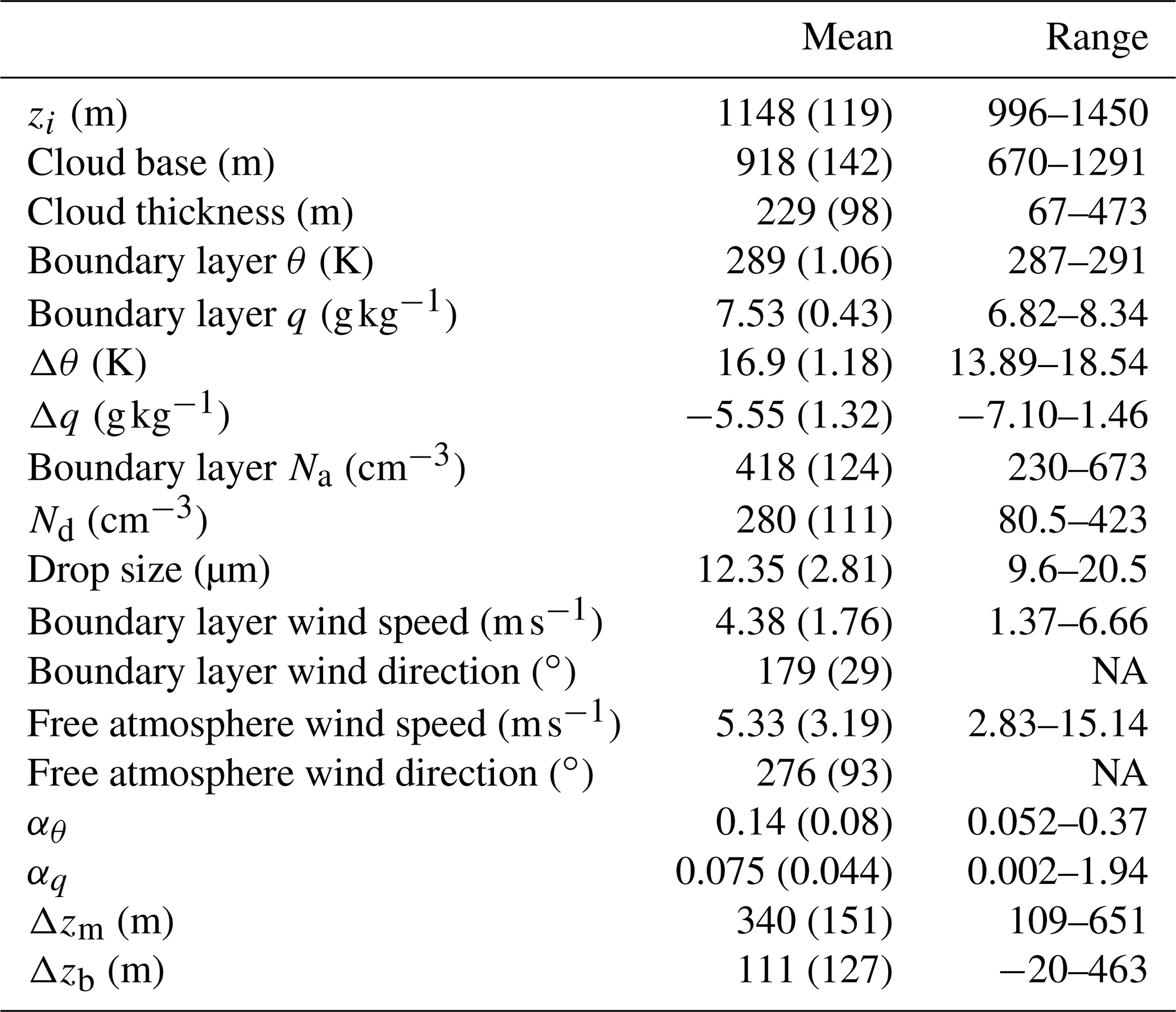
Figure 5 shows vertical profiles (within which the height z is normalized by the inversion height to give a nondimensional vertical coordinate of ) of θ, q, LWC, and Na. Individual flight profiles are in gray, with the red profile representing the mean and the blue profiles representing the flights conducted on 1 (RF11, light blue) and 2 November (RF12, dark blue). Mean profiles show that on average the MBL is well mixed up to the inversion, which then prevents mixing into the free atmosphere above (as evidenced by the decrease in aerosol number concentration between the boundary layer and free atmosphere).
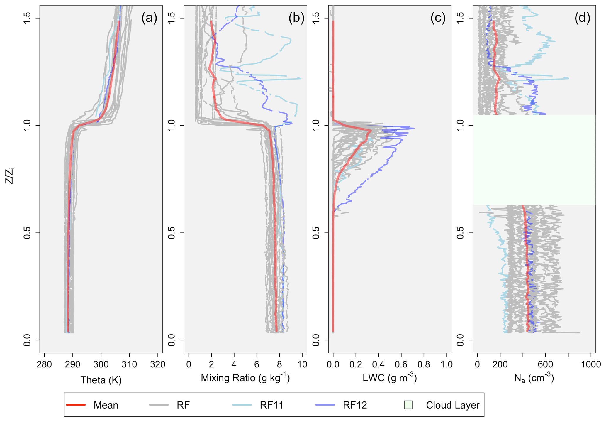
Figure 5Profiles scaled by zi. (a) θ (K); (b) q (g kg−1); (c) LWC (g m−3); (d) Nd (cm−3). The red profile represents the mean value, and the two blue profiles represent RF11 (light blue) and RF12 (dark blue). The green layer represents the relative cloud layer for (d), as aerosol data cannot be collected in the cloud layer.
The largest deviations from the mean in the profiles occur during the passage of the synoptic system on 1 and 2 November. At this time, both RF11and RF12 measured the following: (1) the thickest Sc cloud layer, with 1 November having the largest average cloud droplet size (20.8 µm) and in-cloud drizzle rates, while 2 November had the lowest recorded cloud base and largest recorded LWC; (2) a larger mixing ratio above the boundary layer, which suggests the presence of a moist layer aloft that may have helped to produce the thickest cloud layers observed; and (3) the smallest differences in both θ and q from the bottom to the top of the inversion layer. During the passage of strong events as described by Rahn and Garreaud (2010a), the inversion defining the MBL erodes, making it hard to define zi. This process is partially illustrated by the smaller differences in temperature and moisture across the inversion layer during the passage of the synoptic disturbance.
The differences in q and θ can be better visualized in Fig. 6, which shows the differences between values below and above the inversion in panel (a). values between 0.85 and 0.95 were used for the averages below the inversion, while data between values of 1.10 and 1.20 were used for the averages above the inversion. Besides 1 and 2 November, and to a lesser degree 4 November, the average difference in θ across the inversion was 17 K, while the average difference in q was −6.2 g kg−1. On 1 November when both reached a minimum difference, the difference between q and θ across the inversion was 1.9 g kg−1 and 14 K, respectively, and a weaker inversion allows for more entrainment mixing near cloud top (Galewsky, 2018).
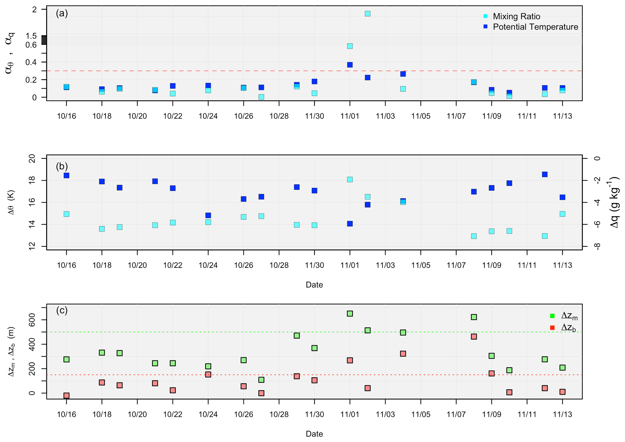
Figure 6(a) θ (left y axis, dark blue) and q (right y axis, light blue) differences across the inversion for all 18 flights. (b) The decoupling parameters for mixing ratio (light blue) and potential temperature (dark blue); the red dashed line represents the 0.30 value. (c) Mixed layer cloud thickness (green) and the difference between cloud base and the LCL (red); the red dashed line represents the 500 value, and the green dashed line represents the 150 value.
To analyze whether the boundary layer is well mixed or decoupled, two methods are used: (1) decoupling parameters and (2) analysis of the expected LCL for a well-mixed layer in relation to actual cloud base. Decoupling parameters αθ and αq depend on the profiles of θ and q, respectively (Wood and Bretherton, 2004). The decoupling parameters measure the relative difference in q and θ between the bottom (near the surface) and top (near the inversion) portions of the boundary layer and are given by
where ( ) is the level ≈25 m above (below) zi, and θ(0) and q(0) are the potential temperature and mixing ratio at the surface. Here, is calculated using data between values of 1.03 and 1.05, while is calculated using data between values of 0.95 and 0.97 (this is roughly 25 m above and below zi, respectively). The closer to zero the decoupling parameters are, the more well mixed the boundary layer is. Previous observations suggest that if the parameters exceed ≈0.30, the boundary layer is decoupled (Albrecht et al., 1995).
Mixed layer cloud thickness represents the difference between zi and the LCL (Δzm) and was found to be strongly correlated with decoupling in Jones et al. (2011). The difference between cloud base (zb) and the LCL represents another decoupling index (Δzb) related to the LCL presented in Jones et al. (2011). Decoupling of the boundary layer occurs when the boundary layer deepens, resulting in a larger difference between the inversion and the LCL as the LCL diverges from cloud base. A well-mixed boundary layer would have zb and LCL measurements in close agreement, while a decoupled boundary layer would have a divergence in the similarities between the two values. Previous observations within the VOCALS-REx domain from Jones et al. (2011) found that the boundary layer tended to be decoupled if Δzb>150 m and if Δzm>500 m.
Figure 6b shows the decoupling parameters. The average values of αθ and αq are 0.14 and 0.08, respectively, both of which are within the regime of well mixed. During RF11 and RF12, q increases above the inversion, leading to large values for αq, while Δθ is relatively small compared to other flights, with αθ being above 0.30 during 1 November (Zheng et al., 2011, suggest that drizzle processes act to stabilize the boundary layer, leading to decoupling). Panel (c) provides values for Δzb and Δzm for each flight, with average values of 111 and 340 m, respectively. Again, both values are within the well-mixed regime.
RF11, RF13, and RF15 are shown to be decoupled, with both Δzb and Δzm at or above the 150 and 500 m threshold values, respectively. RF12 is decoupled according to Δzm only, and RF6 and RF16 are decoupled according to Δzm only. Looking at raw profiles of q and θ (not shown here), RF6, RF11, RF12, RF13, and RF15 appear to be decoupled due to distinct humidity changes within the sub-cloud profiles, including the presence of a cumulus layer below the Sc deck that is visible from analyzing the LWC profiles (not displayed here) during RF11 (8 November). According to these metrics 28 % of the profiles analyzed are decoupled.
The comparison between panels (b) and (c) demonstrates that determining decoupling using Δzb and Δzm appears to be more accurate than the decoupling parameters when comparing the results to the raw vertical profiles. A more accurate value for determining decoupling using αθ and αq for the data presented here is 0.20 compared to the 0.30 stated in Albrecht et al. (1995). A value of 0.20 would lead to better agreement between the two methods. Note that the correlation between Δzb and Δzm is 0.76 (i.e., when the mixed layer cloud thickness increases, the difference between the LCL and cloud base increases). This suggests that when the boundary layer deepens, the cloud layer thickness remains relatively consistent, in agreement with findings from Jones et al. (2011).
Here, we will quantify the amount of turbulence occurring within the boundary layer. In particular, the analysis includes (1) analyzing day-to-day variability in turbulent measurements and boundary layer characteristics by relating them to synoptic changes in meteorological conditions and (2) determining average turbulent values throughout the vertical structure of the STBL by classifying the STBL based on different turbulent profiles analyzed. For each flight analyzed here, the Sc deck lies directly below a strong inversion. It should be noted that this extreme vertical gradient can cause instrument response issues with the measurement of both the dry bulb and dew point temperature for some distance beneath cloud top (Nicholls and Leighton, 1986). Therefore, data collected during both vertical profiles and horizontal legs will be used and compared.
4.1 Synoptic variability of turbulence
Figure 7 shows the mean surface (30 m horizontal flight leg) LHF (panel a), SHF (panel b), and TKE and ϵ (panel c) for each flight day, with the standard deviation represented by the shaded envelopes. Note that for days with two or more mean values, there were two or more 30 m horizontal flight legs, with good agreement between mean leg values within the same flight. The LHF peaks on 26 October with a value of 50.7 W m−2, and from that point it decreases steadily to its minimum values of 19.2 and 18.4 W m−2 on 2 and 4 November, respectively. The SHF has a sharp increase to its maximum value of 17.0 W m−2 on 1 November and decreases to a below-average value of 5.4 W m−2 on 2 November (Table 3). Note that the average surface values of the LHF and SHF are generally in agreement with those found in Zheng et al. (2011), who found mean values of 48.5 and 7.1 W m−2, respectively. The differences most likely arise due to different averaging techniques.
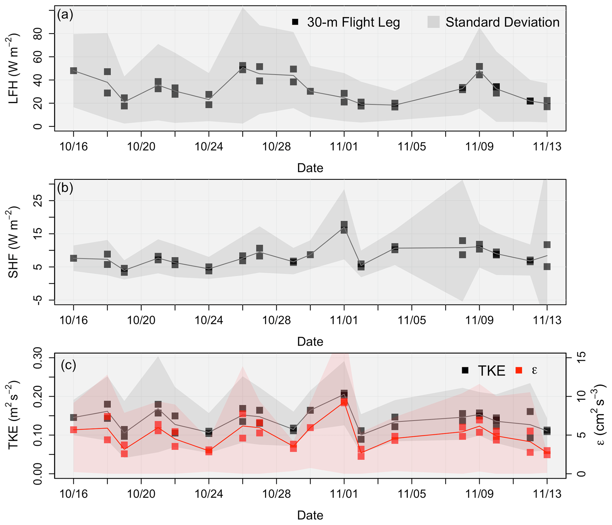
Figure 7Values of (a) surface LHF (W m−2), (b) surface SHF (W m−2), and (c) surface TKE (m2 s−1) in black and surface ϵ (cm2 s−3) in red for each flight day. Each square is a mean of a 30 m horizontal flight leg, while each envelope represents the standard deviation.
Table 3Mean and range of values for select surface variables over the 18 flights analyzed, with the standard deviation and the research flight number in parentheses for column mean and range, respectively.
Surface TKE and ϵ both reach a maximum on 1 November, followed by both reaching a minimum on 2 November (see Table 3 for the mean and range of values). Both TKE and ϵ show very little variation between measurements, except between 30 October and 2 November, when turbulence shows a large increase followed by a rapid decrease. Overall, there is good agreement between mean values within the same flight, with the exception of 12 November for TKE and ϵ and 13 November for the SHF.
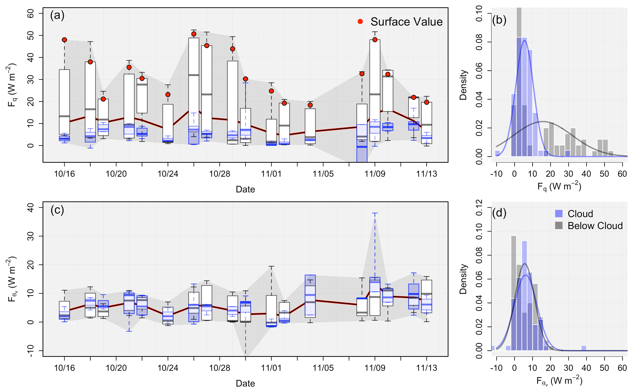
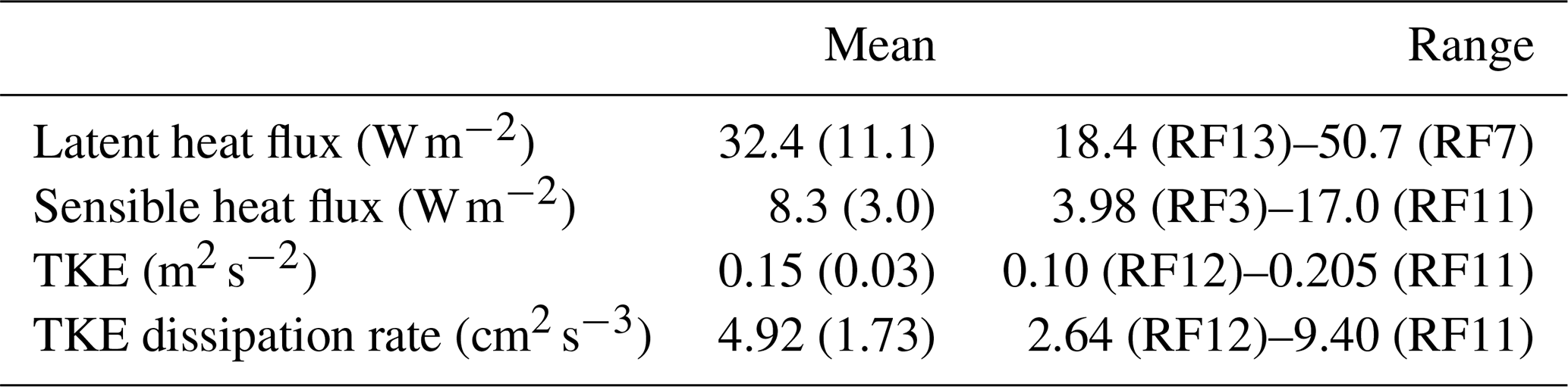
Figure 8Box plots of in-cloud (blue) and sub-cloud (white) data using mean values of horizontal flight legs for (a) Fq (W m−2) and (c) (W m−2). The gray envelope represents the range of the data, while the red line represents the mean value for each flight. Panels (b) and (d) provide the distribution of the data populations (with normal distributions overlaid for reference) for Fq and , respectively.
Shifting focus to the entire depth of the boundary layer, Fig. 8 shows box plots (of leg-mean values) of sub-cloud (white) and in-cloud (blue) values of Fq (panel a) and (panel c). Panels (b) and (d) display histograms of Fq and data, respectively, with normal distribution fits for reference. The overall Fq was 10.63±3.66 W m−2, with a sub-cloud mean of 16.43±6.84 W m−2 and an in-cloud mean of 5.0±3.05 W m−2. The sub-cloud Fq is clearly offset to larger values owing to surface evaporation and subsequent transport of moisture. The red dots in panel (a) represent the surface values, which are always the largest within the entirety of the vertical layer. The lowest mean values occurred on the same days as the minimum in geopotential height, 1 and 2 November, with values of 5.60 and 4.68 W m−2, respectively. Statistically speaking these two datasets (sub-cloud vs. in cloud) are statistically different, with a p value of (note that all statistical significance tests are carried out using the Wilcoxon sum–rank test). Removing the surface 30 m horizontal flight leg data, however, results in these two datasets being statistically similar, with a p value of 0.21.
As demonstrated in panel (c), the overall mean was 5.84±2.86 W m−2, with a sub-cloud value of 5.10±1.99 W m−2 and an in-cloud value of 5.99±4.03 W m−2. Based on the mean flight leg values, there does not appear to be a large difference in between the sub-cloud and in-cloud sections of the boundary layer, which is not as expected. In-cloud buoyancy in general is enhanced due to latent heating and cooling effects. There is no statistically significant difference between the in-cloud and sub-cloud data, with a p value of 0.43. While the medians in the data populations are similar, in-cloud has a clear increase in variance and a much larger range (−13.2 to 38.1 W m−2), suggesting more variation and isolated occurrences of extremely large or small within the cloud compared to sub-cloud (range of −1.7–19.5). Connecting back to concepts discussed in the Introduction, the correlation coefficient between the surface LHF and the in-cloud is 0.34, providing some evidence that a larger surface LHF leads to a larger in-cloud buoyancy flux, as suggested by Bretherton and Wyant (1997) and Lewellen et al. (1996).
Figure 9As in Fig. 8, except for TKE (m2 s−2) in (a) and (b) as well as ϵ () in (c) and (d).
Figure 9 provides the same format as that of Fig. 8, except for TKE (panel a) and ϵ (panel c). The total mean TKE was 0.126±0.03 m2 s−2, with a sub-cloud mean of 0.127±0.04 m2 s−2 and an in-cloud mean of 0.124±0.035 m2 s−2. The total mean ϵ was 3.74±1.34 cm2 s−3, with a sub-cloud mean of 3.87±1.58 cm2 s−3 and an in-cloud mean of 3.50±1.40 cm2 s−3. Overall, very consistent sub-cloud and in-cloud values (when looking at the means) are observed, resulting in statistical similarity between the data populations for both TKE and ϵ. However, in looking at the box plots, one can see that there are several cases (including 24 October and 1 and 2 November) in which the entire turbulent distribution of the sub-cloud data is shifted to larger values than those of in-cloud data, with minimal overlap. This implies that the two layers have limited mixing between them, perhaps due to a more turbulent decoupled lower boundary layer. Along with having different in-cloud and sub-cloud turbulent distributions, both the TKE and the ϵ had maximum average values on 1 November (0.163 m2 s−2 and 6.13 cm2 s−3, respectively) and minimum average values on 2 November (0.065 m2 s−2 and 1.30 cm2 s−3, respectively).
The analysis for this point clearly shows a maximum in turbulent properties on 1 November and a minimum on 2 November. This maximum is driven by turbulence below the cloud but with the in-cloud TKE (0.113 m2 s−2) and ϵ (2.66 cm2 s−3) being below normal for in-cloud values, for which the normal is 0.124 m2 s−2 and 3.50 cm2 s−3, respectively. From Sect. 3.2, it is known that each of the three cases outlined above (24 October, 1 and 2 November) is decoupled. Although 4 and 8 November are also decoupled, these box-plot profiles do not show the same shifted turbulent distributions between the sub-cloud and in-cloud layers. However, 4 and 8 November do have lower-than-average turbulence (all five of the decoupled boundary layers have lower-than-average turbulence, except for 1 November, which will be looked at more closely in Sect. 4.2). There is a strong negative correlation between the variables used to determine decoupling in Sect. 3.2 and the in-cloud turbulence (bottom portion of Table 4), revealing that more decoupled boundary layers correspond to less in-cloud turbulence. The decoupling variables also have a strong positive correlation with zi, indicating that an increase in zi leads to an increased chance of boundary layer decoupling. Negative correlations between in-cloud turbulence and zi reinforce this idea. The increase in zi is accompanied by a decrease in turbulence within the cloud layer. As zi increases, cooling near cloud top cannot sustain mixing over the entire depth of the boundary layer, resulting in less turbulence and boundary layer decoupling (Bretherton and Wyant, 1997).
Along with analyzing correlations between zi, turbulence, and decoupling, it is important to analyze other turbulent fluxes of energy, momentum, and moisture as they act to determine boundary layer structure and characteristics, along with analyzing how these variables are related to synoptic-scale properties such as geopotential height. The correlation coefficients between boundary layer characteristics and synoptic-scale properties can be found in the top portion of Table 4. The 700 hPa geopotential height (i.e., pressure) is strongly correlated with zi, although this correlation is negative with a value of −0.49, suggesting that as the pressure increases, zi decreases. The rate of change in zi is governed by the entrainment rate (ωe) and omega (ω, i.e., vertical velocity in pressure coordinates). If the rate of subsidence increases to the point that it is larger than ωe, then zi will decrease with time. ω depends primarily on synoptic-scale patterns, in particular that of geopotential height. Pressure and ω have a correlation of −0.71, suggesting that as pressure increases, the subsidence increases (or at the very least, upward vertical motion is diminished). Entrainment, on the other hand, can depend on multiple variables, including the inversion layer thickness, wind shear, and surface fluxes. Increases in ωe result in a higher LCL for the entrained air and a resulting increase in boundary layer height. Given that zi decreases as the pressure increases, this suggests that subsidence becomes the dominating component that governs zi rather than entrainment.
Table 4Correlation coefficient values in the right column and variables in the left column, with ↔ dividing the variables being compared. GPH is geopotential height (i.e., a proxy for pressure). Values with * were calculated excluding RF11 and RF12 due to the increase in mixing ratio above zi, resulting in abnormally large αq values.
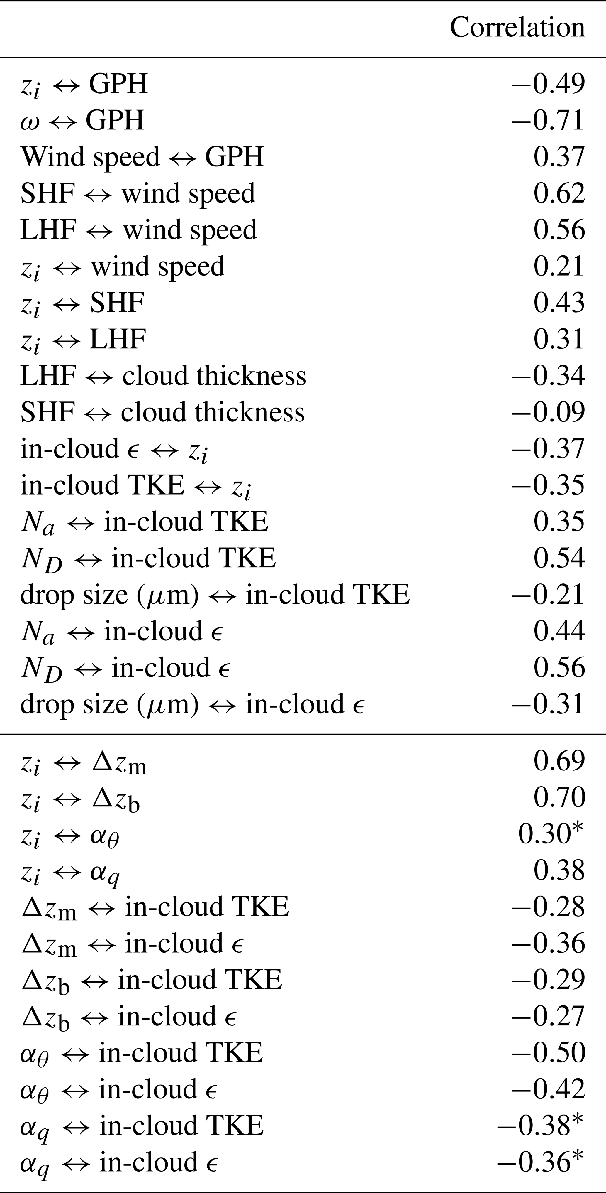
The surface LHF provides the main source of moisture in the STBL, which in turn is an important source of buoyant TKE production. An enhanced (reduced) LHF will generate thicker (thinner) clouds with larger (smaller) LWC values, resulting in enhanced (reduced) evaporative cooling near cloud top and leading to enhanced (reduced) buoyancy-driven entrainment, with a subsequent deepening (thinning) of the boundary layer. This process is demonstrated well when analyzing the correlation coefficients. Both the LHF and SHF are positively correlated with zi (correlation coefficients of 0.31 and 0.43, respectively), while the LHF is negatively correlated with the Sc cloud thickness (correlation coefficients of −0.34). Therefore, a larger LHF tends to result in a thinner Sc cloud layer but a larger zi, suggesting that enhanced entrainment acts to thin the cloud layer while deepening the boundary layer. It should also be noted that the correlation between the SHF and wind speed is significant, as anticipated, since the SHF is expected to increase linearly with wind speed (Palm et al., 1999).
As Nd and Na increase (accompanied by a decrease in average droplet size), the TKE and ϵ increase (with correlation coefficients of 0.35, 0.54, and −0.21 in relation to TKE, respectively). As precipitation is suppressed due to larger number concentrations and smaller droplet sizes, a reduced moisture loss from the STBL can result, leading to thicker clouds, a larger buoyancy flux, and a larger TKE. Smaller droplets will also evaporate more readily, leading to enhanced in-cloud latent heating (i.e., absorption of energy through evaporation) and a resultant increase in turbulence through the buoyancy flux.
4.2 Vertical profiles
It has been shown through the boundary layer vertical structure in Fig. 5 that the boundary layer is, on average, well mixed when considering thermodynamic variables. Using data collected during aircraft soundings (as opposed to mean values of horizontal flight legs), u variance (), v variance (), vertical velocity variance (), and the TKE are displayed in Fig. 10a to d, respectively, with the red line representing the mean profile and each gray line representing individual flight profiles. The blue lines represent flight profiles for 1 (light blue) and 2 November (dark blue). Panel (e) displays the mean values from panels (a) through (d), along with the anisotropy ratio (). The profile of each variable in question shows a nearly constant value below cloud base, with an in-cloud increase before beginning to decrease near cloud top. Both and TKE reach their peak values at (or a normalized in-cloud height, Z*, of 0.43). TKE values plummet above the inversion due to the dominance of clear, stable, and subsiding air aloft. The overall maximum in TKE measured (for all 18 flights) is found near (looking at the light blue profile line in Fig. 10d) during RF11 (1 November). This will be discussed in more detail in Sect. 4.3.
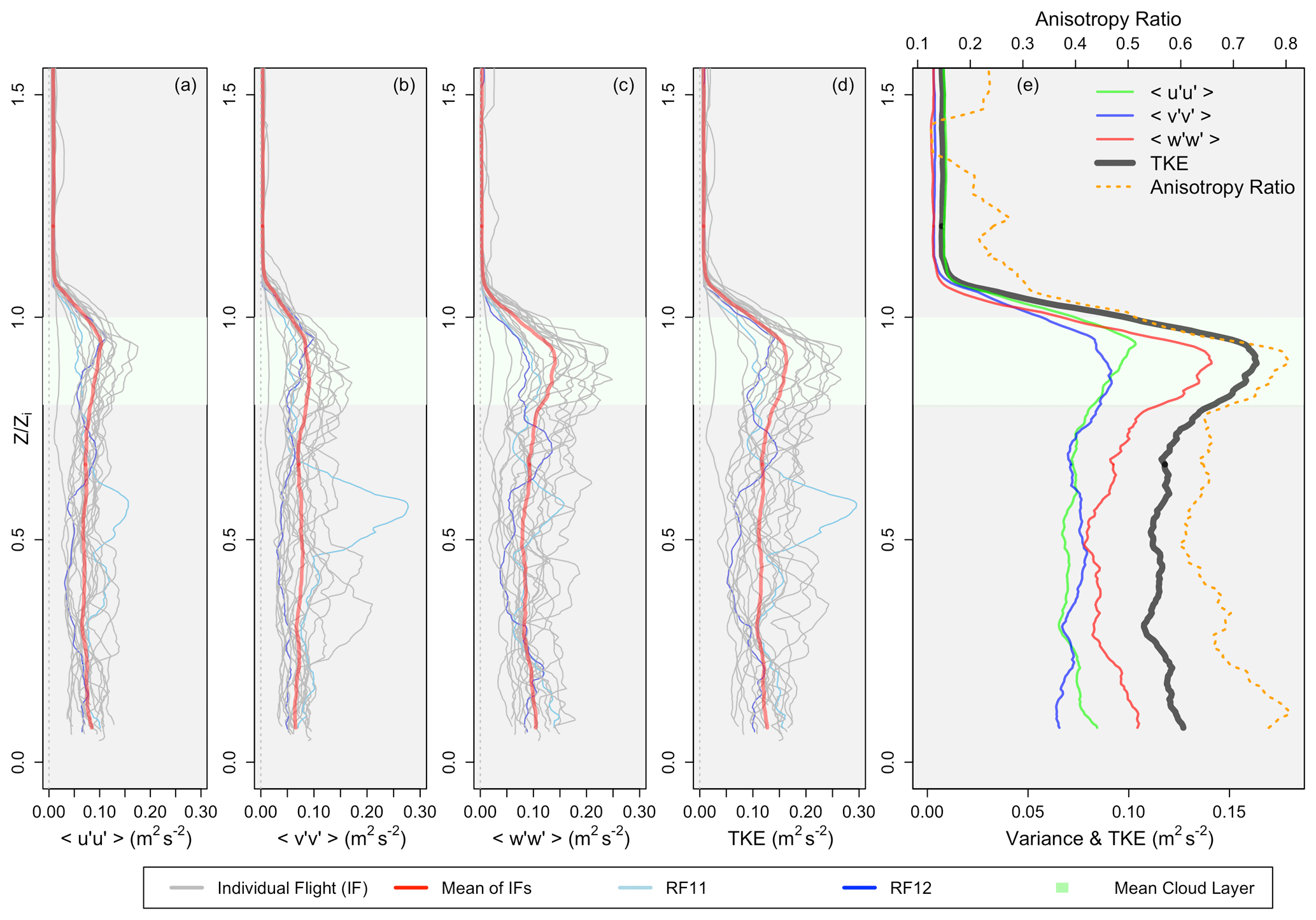
Figure 10Vertical profiles (from data collected during flight profiles) of (a) u variance (m2 s−2), (b) v variance (m2 s−2), (c) w variance (m2 s−2), and (d) TKE (m2 s−2). Individual flights are displayed in gray, and the mean value is displayed in red, with RF11 and RF12 shown in light blue and dark blue, respectively. (e) Mean values from (a) through (d), along with the anisotropy ratio in orange.
The observed average in-cloud at Point Alpha was 0.127±0.051 m2 s−2, with values fluctuating considerably more than those in the sub-cloud layer (0.091±0.025 m2 s−2, in agreement with findings from Bretherton et al., 2010, who measured a larger standard deviation in in-cloud vs. sub-cloud vertical velocity). As is found here, Hignett (1991), Nicholls (1984), and Ghate et al. (2014) also found that peaked in the upper half of the STBL away from any boundaries such as cloud top. Overall, the flow is not isotropic (the anisotropy ratio is equal to 1 for isotropic flow; vertical turbulence dominates for values greater than 1, and horizontal turbulence dominates for values less than 1). Vertical turbulence has its largest component near the surface (), while having a secondary in-cloud peak in accordance with the peak in TKE at .
Simulations and observations from Pasquier and Jonas (1998) of in-cloud TKE showed that the maximum TKE occurred in two locations, near cloud top and near cloud base, suggesting that turbulence is being generated through two processes: (1) cooling at or near cloud top (through evaporation or longwave cooling), resulting in cool, dry downdrafts; and (2) warming near cloud base from the release of latent heat through condensation, resulting in positively buoyant updrafts. Looking at individual profiles of TKE (not shown here), only 8 of the 18 flights have a maximum TKE within the cloud layer. Modeling and observations of boundary layer profiles of turbulence from Pasquier and Jonas (1998) showed that mixing and overturning of the boundary layer profile due to buoyancy effects leads to a maximum in turbulence commonly being reached in the sub-cloud layer. A total of 10 of the 18 flights display two peaks in TKE within the cloud layer, one near cloud base and another near cloud top, signifying evaporative cooling near cloud top and latent heating near cloud base. Of the eight flights that have a maximum TKE within the cloud layer, all eight display two peaks in the TKE within the cloud layer, one near cloud base and one near cloud top. Having the maximum in TKE in the sub-cloud layer can signify decoupling (Durand and Bourcy, 2001). A slight decoupling can lead to less moisture transport into the Sc layer, resulting in less latent heat release due to condensation. This could be why only two flights have two peaks in TKE within the cloud when the turbulence maximum is reached below cloud due to latent heat release at cloud base being suppressed. All decoupled flights identified in Section 3.2 (with the exception of 1 and 2 November) have a single peak in TKE in the cloud layer, with the maximum TKE value being reached within the sub-cloud layer.

Figure 11Vertical profiles (from data collected during flight profiles) of (a) (W m−2), (b) Fq (W m−2), and (c) vertical velocity skewness (m3 s−3). The red line is the smoothed average of the raw data (black), while the gray envelope represents the range of values encountered.
Figure 11 provides the same format as Fig. 10, except for values of (panel a), Fq (panel b), and vertical velocity skewness (panel c). Note that Fig. 11 displays the range of data in the gray envelope, as opposed to showing each individual profile with a single gray line. has a maximum value at (). The peak near cloud middle is due to a combination of the warm–moist updrafts and cool–dry downdrafts meeting, formed by evaporative cooling at cloud top and latent heating near cloud base. According to Pasquier and Jonas (1998), should reach a minimum near cloud top from the entrainment of warm, dry air down into the cloud layer. Although the mean profile does not show a decrease at cloud top, the raw data (i.e., unsmoothed) do show a negative buoyancy flux at cloud top. For individual flights, only RF11 (1 November) had a maximum in in the sub-cloud layer. Fq peaks at the surface but also sees a secondary maximum at . The maximum at cloud top can be attributed to the strong q gradient and to entrainment of drier air down into the cloud (i.e., also a positive flux since both w′ and q′ are negative).
Well-mixed STBLs tend to show characteristics of downdrafts that are spatially smaller but stronger than updrafts. This results in a negative vertical velocity skewness (from here on ) through most of the cloud and sub-cloud layer (Nicholls, 1989; Hogan et al., 2009; Ghate et al., 2014). Panel (c) indicates that on average is negative throughout the cloud layer and through most of the sub-cloud layer, having a maximum value near the surface. The minimum value in occurs at cloud base (), suggesting that overall, the downdrafts are spatially smallest yet strongest at cloud base, while updrafts are spatially largest but weakest.
4.3 RF11 (1 November)
Turbulent and boundary layer characteristics have been shown to be abnormal on 1 November, with a minimum in 500 hPa geopotential height, Na, and Nd. 1 November also had overall mean maximum values of TKE and ϵ within the sub-cloud layer, along with maximum values in the surface SHF and in-cloud drizzle rate. The average in-cloud drizzle rate on 1 November was the largest recorded (a mean in-cloud drizzle water content of 0.025 g m−3 measured by the cloud-imaging probe – CIP) and roughly 4.5 times that of the second-largest in-cloud average recorded on 2 November (0.0055 g m−3), when the average for all other flights was 0.0014 g m−3. A moist layer is present above the boundary layer from looking at profiles of q in Fig. 5, leading to the secondary maximum in LWC and cloud thickness (2 November had the largest cloud thickness and LWC). Also visible in Fig. 3 is the presence of wind shear near .
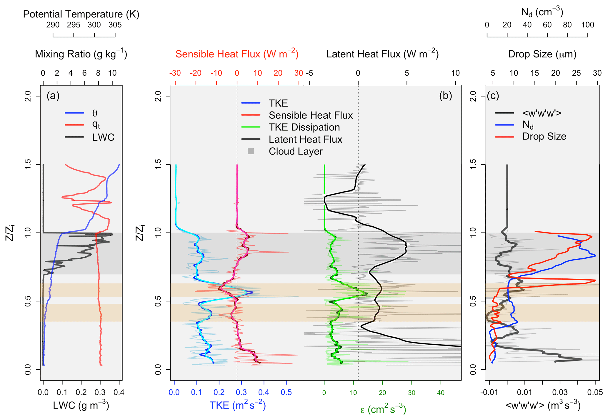
Figure 12Vertical profiles as functions of normalized boundary layer height for RF11 (1 November) of (a) θ (K) in blue, q (g kg−1) in red, LWC (g m−3) in black, (b) TKE (m2 s−2) in blue, Fθ (W m−2) in red, ϵ (cm2 s−3) in green, and Fq (W m−2) in black. The thin light-colored lines represent raw values, while the dark thick lines represent smoothed averages; (c) (m3 s−3) in black, Nd (cm−3) in blue, and the corresponding average droplet size (µm) in red. The gray envelope represents the cloud layer, and the orange envelopes represent areas of interest (main location of decoupling and evaporation).
In order to explore this case further, Fig. 12 shows profiles of multiple thermodynamic and turbulent variables as a function of . Panel (a) shows profiles of θ (blue), LWC (black), and q (red). The gray envelope represents the cloud layer, while the orange envelopes represent areas in the sub-cloud layer where Fθ is negative and TKE and ϵ are enhanced. The potential temperature at the base of the lowest orange envelope begins to deviate from its surface value and increases steadily up to the inversion, indicating significant entrainment of the warmer, less buoyant air aloft down to . However, q within the boundary layer stays relatively constant. This is due to the fact that the entrainment of the warmer air aloft has a larger q than that near the surface of the boundary layer. Significant decoupling is occurring in the sub-cloud layer near (the largest TKE and ϵ are located) and 0.40 (secondary maximum in the TKE and ϵ). It is suggested here that precipitation from the Sc deck acts to decouple the boundary layer and enhance sub-cloud turbulence due to evaporative cooling occurring primarily in the regions outlined by the orange envelopes.
Several variables must be considered here. First, the moist layer above the Sc deck can have two effects: (1) changing the radiative balance at cloud top through increased downwelling longwave radiation (Christensen et al., 2013) and (2) entrainment of more moist air near cloud top, reducing evaporational cooling that would otherwise occur through the entrainment of drier air (Eastman et al., 2017). Both effects act to reduce cooling (both evaporational and radiational) near cloud top, slowing the rate of boundary layer deepening through decreases in entrainment. Eastman and Wood (2018) found that high humidity above the Sc deck acts to slow boundary layer deepening, while the entrainment of increased water vapor into the boundary layer results in enhanced cloud cover.
Second, drizzle can have multiple effects on boundary layer structure, including the following: (1) precipitation removes liquid water from the Sc deck, resulting in cloud thinning if the surface LHF is not large enough to maintain the Sc deck (Austin et al., 1995); (2) warming of the drizzle-producing cloud layer occurs through latent heating, acting to stabilize the cloud layer; (3) changing the stability of the sub-cloud layer depends on the profile of sub-cloud evaporation. Significant proportions of precipitation are known to evaporate before reaching the surface (Comstock et al., 2004; Wood et al., 2015; Zhou et al., 2015), and where this evaporation occurs determines whether the layer will become more or less unstable. When precipitation is heavier and in the form of large drops it tends to stabilize the boundary layer from evaporational cooling spread over the depth of the sub-cloud layer, with substantial evaporation near the surface stabilizing the boundary layer. When precipitation is lighter and in the form of small drops, cooling persists in the uppermost part of the sub-cloud region, resulting in destabilization of the sub-cloud layer (Feingold et al., 1996; Wood, 2005, 2012; Mechem et al., 2012; Rapp, 2016; Ghate and Cadeddu, 2019).
Here, precipitation promotes STBL decoupling by reducing the diabatic cooling in the cloud layer through in-cloud latent heating, resulting in a stabilization of the cloud layer (the average in-cloud turbulence on 1 November is the fifth-lowest measured, while 2 November is the lowest measured; see Fig. 9). The sub-cloud evaporation leads to cooling below cloud, and a resultant local minimum in the buoyancy flux is created (Bretherton and Wyant, 1997). It is known from Wood (2005) that evaporative cooling shows cooler and more moist characteristics than non-precipitating regions. Fθ is observed to be negative from up to cloud base, with the minimum and local minimum outlined by the orange envelopes. Fq is also shown to be slightly enhanced within these regions (i.e., an enhanced source of vapor from evaporation). This suggests that evaporational cooling is occurring in these regions, resulting in the largest average turbulence being measured in the sub-cloud layer on this day due to sub-cloud destabilization. It was mentioned earlier that Zheng et al. (2011) suggested that drizzle processes act to stabilize the boundary layer, leading to decoupling. This is partially true, as precipitation does lead to decoupling; however, the precipitation actually destabilized the sub-cloud layer while stabilizing the cloud layer.
Normally, the process just explained will result in the cloud layer being decoupled form the surface moisture source, leading to a thinning cloud layer. However, the Sc deck is receiving moisture from the upper atmosphere (as seen in the negative Fq above cloud, where w′ is negative but q′ is positive). This process acts to moisten the boundary layer, which will lower the LCL, and assuming that zi does not change, this will thicken the cloud (Randall, 1984). Note that the cloud layer on 2 November is thicker than that on 1 November by roughly 100 m, while zi is roughly 50 m lower.
Looking at panel (c), Nd is provided by the phase Doppler interferometer (see Chuang et al., 2008, for more information), which provides a time series of droplet arrival times with no instrumentation dead time. The average drop size is also provided. The average in-cloud (sub-cloud) drop size is 20.7 µm (6.49 µm). The average drop size below cloud base and above the top orange envelope is 26.0 µm (the maximum value for the profile). The average in-cloud (sub-cloud) Nd is 81.7 cm−3 (15.23 cm−3). Nd below the bottom orange envelope is 7.15 cm−3, whereas Nd above the bottom orange envelope to cloud base is 25.33 cm−3. Two conclusions can be inferred from panel (c): (1) the rapid evaporation of large drops within the first orange envelope () and (2) the evaporation of a majority of the remaining smaller droplets within the second orange envelope (), reinforcing the fact that evaporation away from the boundary layer surface results in decoupling while enhancing sub-cloud turbulence. Note that also varies between positive and negative values within the sub-cloud layer, providing more evidence that decoupling is occurring.
To summarize, it appears that the sub-cloud layer is decoupled from the Sc deck due to the evaporative cooling of precipitation. This increases turbulence within the sub-cloud layer while reducing turbulence in the cloud layer. However, the cloud layer is still supplied with moisture through the entrainment of the more moist air aloft, driving cloud deepening and sustaining the Sc deck. The wind direction shifts from the south in the lower portion of the boundary layer to northerly near Note that the maximum value in TKE that is measured on 1 November at (see the light blue profile line in Fig. 10) matches the location at which the wind shear occurs. However, this spike in TKE cannot be attributed to the wind shear alone, as wind shear that occurs at the inversion for each flight day and within the boundary layer on 4 November does not result in large increases in turbulence. The increase in turbulence seen on 1 November is related to latent heating and the resulting changes in the buoyancy fluxes.
Although not displayed here, profiles for 2 November (the day with the lowest average turbulence, both in cloud and sub-cloud) show a very consistent turbulent profile (no large spikes within or below the cloud layer). It is suggested here that between 1 and 2 November one of two things occurred: either (1) precipitation stopped (i.e., the source of instability in the sub-cloud layer) and enhanced turbulent mixing of the sub-cloud layer ceased (while the cloud layer continued to deepen from the entrainment of more moist air, reducing the LCL), or, the more likely candidate, (2) precipitation continued to occur, leading to evaporation near the surface and a stabilization of the entire boundary layer (there is evidence that a few droplets have already reached the surface in Fig. 12c). Although in-cloud drizzle occurs (stabilizing the cloud layer through latent heating) on 2 November, there is no evidence of sub-cloud evaporation or drizzle. Therefore, there are limited sources of turbulent production until drier air moves in and enhanced entrainment cooling near cloud top can resume mixing of the boundary layer, or precipitation restarts and acts to destabilize the sub-cloud layer. It should be noted that although attention has been brought to 1 and 2 November throughout the paper (due to the passing synoptic system leading to unique characteristics that warranted further investigation), these two flight days do fit the overall correlations presented in Table 4.
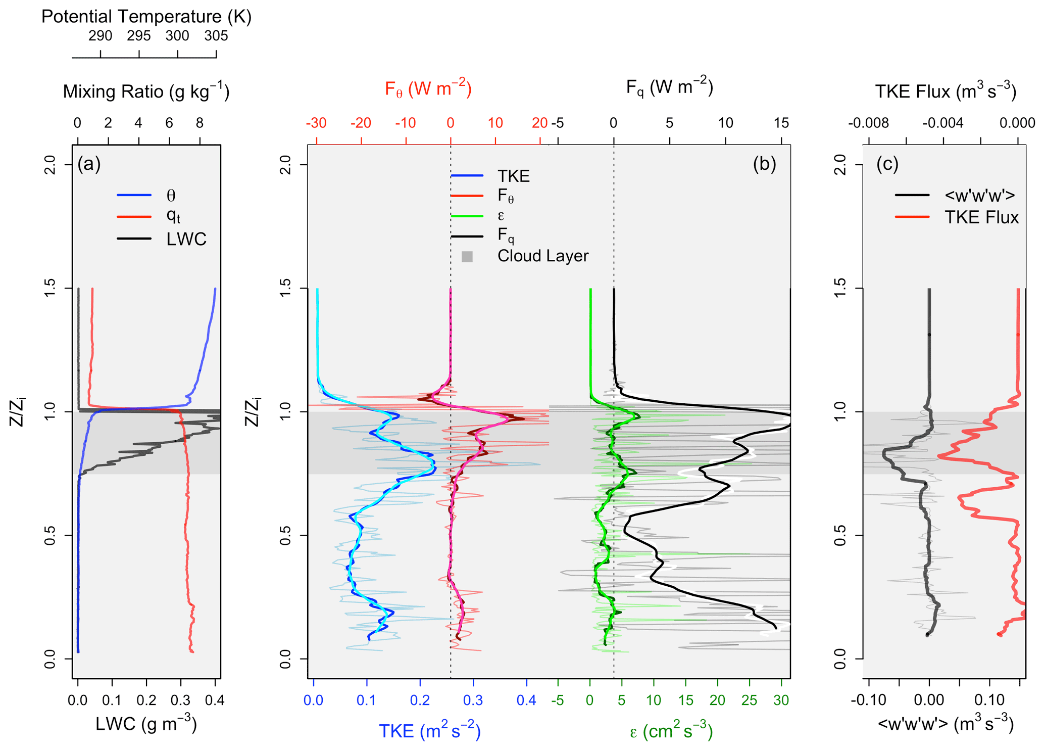
Figure 13As in Fig. 12, except for the well-mixed boundary layer case of RF3 (19 October). Panel (c) provides a profile of TKE flux (m3 s−3) as opposed to N and average drop size.
In Fig. 13 (same format as Fig. 12), a well-mixed boundary layer in RF03 (19 October) is analyzed. Also, note that panel (c) provides the TKE flux as opposed to Nd and drop size (since there is no sub-cloud precipitation to analyze). Both θ and q appear to be well mixed throughout the boundary layer, with a slight decrease in θ throughout the cloud layer. TKE, ϵ, Fq, and Fθ all have two peaks, one near cloud base and one near cloud top, suggesting latent heating near cloud base and evaporative cooling near cloud top. Fθ also has a negative value above cloud top due to the entrainment of warm, dry air down into the cloud. The vertical velocity skewness has a maximum negative value near cloud base and never has an increase to positive values. The negative TKE flux within the cloud layer suggests that upward-moving air is transporting less TKE than downward-moving air (i.e., the main source of turbulence is from entrainment mixing near cloud top, resulting in evaporative cooling).
Variations in turbulent and meteorological properties within the boundary layer on a flight-by-flight basis (synoptic variation) have been examined. It has been shown that the influence of a synoptic system on 1 and 2 November leads to a deepening of the cloud layer during passage due to a moist layer directly above the boundary layer. A large increase in zi is observed after passage. Although the pressure increases (and subsidence becomes stronger) after the passage of the synoptic system, it is proposed that the moist layer above the boundary layer limits boundary layer deepening due to reduced evaporational and radiational cooling near cloud top, limiting entrainment (counteracting the fact that subsidence is weaker). As the synoptic system passes and the upper atmosphere dries, cloud-top cooling is enhanced and entrainment acts to increase zi, counteracting the fact that subsidence is increasing. Analysis over the observation period indicates the following.
-
As the pressure decreases (increases), zi increases (decreases), accompanied by a decrease (increase) in in-cloud turbulence. As zi increases, the chance of boundary layer decoupling increases due to cooling near cloud top being unable to sustain mixing over the entire depth of the boundary layer, resulting in less turbulence and decoupling compared to a shallow, well-mixed boundary layer.
-
Correlation coefficients indicate that as the LHF and SHF increase, zi increases. When the LHF increases, however, the cloud thickness tends to decrease. A larger LHF tends to produce thinner Sc clouds but a larger zi, suggesting that enhanced entrainment at cloud top generated by the larger LHF (through more moisture being available for evaporation) acts to thin the cloud layer while deepening the boundary layer.
-
A maximum in TKE on 1 November (both the overall average and largest single value measured) is due to precipitation acting to destabilize the sub-cloud layer (through evaporation occurring away from the surface, primarily near and ) while acting to stabilize the cloud layer. This is observed in the vertical profiles of RF11 and the TKE and ϵ values in Fig. 9, where it is shown that the distributions of the turbulent data for the sub-cloud and in-cloud layers are completely offset from one another, with the TKE in the sub-cloud layer maximizing for the analysis period, while the TKE in the in-cloud layer is below the average value for the analysis period. 2 November has the lowest average turbulence measured (both in cloud and sub-cloud), which is believed to be a result of (1) lack of cooling near cloud top due to the enhanced moist layer above and (2) heavy precipitation from the previous day (or sometime prior to the measurements being made) leading to evaporation through the entire sub-cloud layer, stabilizing it.
-
A total of 8 of the 18 flights have a maximum TKE within the cloud layer; 10 of the 18 flights display two peaks in TKE within the cloud layer, one near cloud base and another near cloud top, signifying evaporative cooling near cloud top and latent heating near cloud base. Of the eight flights that have a maximum TKE within the cloud layer, all eight display two peaks in the TKE within the cloud layer, one near cloud base and one near cloud top. This suggests that enhanced turbulence below the cloud can act to reduce latent heating and cooling effects within the cloud layer, which generate turbulence near cloud top and bottom. Enhanced sub-cloud turbulence (compared to in-cloud turbulence) could be an initial indicator that the process of boundary layer decoupling has begun but has not developed to the point that classical measurement techniques (like those discussed in Sect. 3.2) can measure the decoupling. All five of the decoupled flights, with the exception of 1 and 2 November, have a single peak in TKE in the cloud layer, with the maximum TKE value being reached within the sub-cloud layer.
-
Analyzing different layers of turbulence over the 18 flights shows that the vertical velocity variance, TKE, and the buoyancy flux, on average, all reach maximum values near cloud middle (Z* between 0.25 and 0.75).
The results presented here represent a snapshot of data through 18 aircraft flights, with at least a day between any two flights. Therefore, the results presented represent boundary layer conditions that were present at the time of measurement, limiting any analysis of continuously evolving boundary layer and turbulent conditions. For example, being able to analyze the changing thermodynamic and dynamic conditions that resulted in large turbulent changes between 1 and 2 November would be ideal, especially since multiple papers have called for observational studies to assess the impact of drizzle-evaporation-induced cooling on boundary layer turbulence (Wood et al., 2016; Zheng et al., 2016, 2017).
All cabin data from different aircraft platforms can be found on the VOCALS-REx website at https://archive.eol.ucar.edu/projects/vocals/rex.html (UCAR, 2008a). The aircraft measurement data during VOCALS-REx were obtained from the public FTP at http://data.eol.ucar.edu/master_list/?project=VOCALS (UCAR, 2008b). The navigation and state parameters are available from https://data.eol.ucar.edu/dataset/89.132 (Albrecht, 2011a). The aerosol data are available from https://data.eol.ucar.edu/dataset/89.158 (Albrecht, 2011b). All NCEP/NCAR reanalysis data can be obtained from NOAA at https://www.esrl.noaa.gov/psd/data/gridded/data.ncep.reanalysis.html (Kalnay et al., 1996).
DSD and JDSG contributed equally to both the analysis and the writing of this paper.
The authors declare that they have no conflict of interest.
We thank the CIRPAS Twin Otter crew and personnel, including pilots Mike Hubble and Chris McGuire, for their effort and support during the field program, along with any individual who contributed to the planning and execution of VOCALS-REx. A special thank you to both reviewers, whose advice helped produce a much improved final product.
This research has been supported by NASA (NESSF – NASA Earth and Space Science Fellowship) (grant no. 80NSSC18K1406).
This paper was edited by Philip Stier and reviewed by two anonymous referees.
Ackerman, A. S., van Zanten, M. C., Stevens, B., Savic-Jovcic, V., and Bretherton, C. S.: Large-eddy simulations of a drizzling, stratocumulus-topped marine boundary layer, Mon. Weather Rev., 137, 1083–1110, 2009. a, b
Akinlabi, E. O., Waclawczyk, M., Mellado, J. P., and Malinowski, S. P.: Estimating Turbulence Kinetic Energy Dissipation Rates in the Numerically Simulated Stratocumulus Cloud-Top Mixing Layer: Evaluation of Different Methods, J. Atmos. Sci., 76, 1471–1488, 2019. a
Albrecht, B.: CIRPAS Twin Otter Navigation and State Parameters, Version 1.0, UCAR/NCAR – Earth Observing Laboratory, available at: https://data.eol.ucar.edu/dataset/89.132 (last access: 3 February 2021), University of Miami, 2011a. a
Albrecht, B.: CIRPAS Twin Otter PCASP Data, Version 1.0, UCAR/NCAR – Earth Observing Laboratory, available at: https://data.eol.ucar.edu/dataset/89.158 (last access: 3 February 2021), University of Miami, 2011b. a
Albrecht, B., Randall, D. A., and Nicholls, S.: Observations of marine stratocumulus during FIRE, B. Am. Meteorol. Soc., 69, 619–626, 1988. a, b
Albrecht, B. A., Penc, R. S., and Schubert, W. H.: An observational study of cloud-topped mixed layers, J. Atmos. Sci., 42, 800–822, 1985. a
Albrecht, B. A., Jensen, M. P., and Syrett, W. J.: Marine boundary layer structure and fractional cloudiness, J. Geophys. Res., 100, 14209–14222, 1995. a, b, c
Austin, P., Wang, Y., Pincus, R., and Kujala, V.: Precipitation in stratocumulus clouds: Observations and modeling results, J. Atmos. Sci., 52, 2329–2352, 1995. a
Blot, R., Clarke, A. D., Freitag, S., Kapustin, V., Howell, S. G., Jensen, J. B., Shank, L. M., McNaughton, C. S., and Brekhovskikh, V.: Ultrafine sea spray aerosol over the southeastern Pacific: open-ocean contributions to marine boundary layer CCN, Atmos. Chem. Phys., 13, 7263–7278, https://doi.org/10.5194/acp-13-7263-2013, 2013. a
Bretherton, C. S. and Wyant, M. C.: Moisture transport, lower-tropospheric stability, and decoupling of cloud-topped boundary layers, J. Atmos. Sci., 54, 148–167, 1997. a, b, c, d, e, f, g, h, i
Bretherton, C. S., Uttal, T., Fairall, C. W., Yuter, S. E., Weller, R. A., Baumgardner, D., Comstock, K., Wood, R., and Raga, G. B.: The Epic 2001 Stratocumulus Study, B. Am. Meteorol. Soc., 85, 967–977, 2004. a
Bretherton, C. S., Uchida, J., and Blossey, P.: Slow manifolds and multiple equilibria in stratocumulus-capped boundary layers, J. Adv. Model. Earth Syst., 2, 14, https://doi.org/10.3894/JAMES.2010.2.14, 2010. a, b, c
Chamecki, M. and Dias, N. L.: The local isotropy hypothesis and the turbulent kinetic energy dissipation rate in the atmospheric surface layer, Q. J. R. Meteorol. Soc., 130, 2377–2752, 2004. a
Christensen, M. W., Carrio, G. G., Stephens, G. L., and Cotton, W. R.: Radiative impacts of free-troposphere clouds on the properties of marine stratocumulus, J. Atmos. Sci., 70, 3102–3118, 2013. a
Chuang, P. Y., Saw, E. W., Small, J. D., Shaw, R. A., Sopperley, C. M., Payne, G. A., and Bachalo, W. D.: Airborne Phase Doppler Interferometry for Cloud Microphysical measurements, Aerosol Sci. Technol., 42, 685–703, 2008. a
Comstock, K., Yuter, S., and Wood, R.: Reflectivity and rain rate in and below drizzling stratocumulus, Q. J. R. Meteorol. Soc., 130, 2891–2919, 2004. a
de Roode, S. R. and Duynkerke, P. G.: Dynamics of cumulus rising into stratocumulus as observed during the first “Lagrangian” experiment of ASTEX, Q. J. R. Meteorol. Soc., 122, 1597–1623, 1996. a
Devenish, B. J., Bartello, P., Brenguier, J.-L., Collins, L. R., Grabowski, W. W., Ijzermans, R. H. A., Malinowski, S. P., Reeks, M. W., Vassilicos, J. C., Wang, L.-P., and Warhaft, Z.: Droplet growth in warm turbulent clouds, Q. J. R. Meteorol. Soc., 138, 1401–1429, 2012. a
Durand, P. and Bourcy, T.: Observations Of The Turbulence Structure Within Two Stratocumulus-Topped, Marine Boundary Layers, Boundary Layer Meteorol., 99, 105–125, 2001. a
Eastman, R. and Wood, R.: The competing effects of stability and humidity on Subtropical Stratocumulus Entrainment and Cloud Evolution from a Lagrangian Perspective, J. Atmos. Sci, 75, 2563–2578, 2018. a
Eastman, R., Wood, R., and O, K. T.: The subtropical stratocumulus-topped planetary boundary layer: A climatology and the Lagrangian evolution, J. Atmos. Sci., 74, 2633–2656, 2017. a
Engeln, A. V. and Teixeira, J.: A planeltary boundary layer height climatology derived from ECMWF Reanalysis Data, J. Clim., 26, 6575–6590, 2013. a
Feingold, G., Stevens, B., Cotton, W. R., and Frisch, A. S.: The relationship between drop in-cloud residence time and drizzle production in numerically simulated stratocumulus clouds, J. Atmos. Sci., 53, 1108–1112, 1996. a
Feingold, G., Koren, I., Yamaguchi, T., and Kazil, J.: On the reversibility of transitions between closed and open cellular convection, Atmos. Chem. Phys., 15, 7351–7367, https://doi.org/10.5194/acp-15-7351-2015, 2015. a
Frisch, U.: Turbulence – The Legacy of A. N. Kolmogorov, Cambridge University Press, New York, USA, 1995. a
Galewsky, J.: Using stable isotops in water vapor to diagnose relationships between lower-tropospheric stability, mixing, and low-cloud cover near the island of Hawaii, Geophys. Res. Lett., 45, 297–305, 2018. a
Garreaud, R. D. and Rutllant, J.: Coastal Lows along the Subtropical West Coast of South America: Numerical Simulation of a Typical Case, Mon. Weather Rev., 131, 891–908, 2003. a
Gesso, S. D., van der Dussen, J. J., Siebesma, A. P., de Roode, S. R., and Boutle, I. A.: A single-column model intercomparison on the stratocumulus representation in present-day and future climate, J. Adv. Model. Earth Syst., 7, 617–647, 2015. a
Ghate, V. P. and Cadeddu, M. P.: Drizzle and Turbulence Below Closed Cellular Marine Stratocumulus Clouds, J. Geophys. Res.-Atmos., 124, 5724–5737, 2019. a, b
Ghate, V. P., Albrecht, B. A., Miller, M. A., Brewer, A., and Fairall, C. W.: Turbulence and Radiation in Stratocumulus-Topped Marine Boundary Layers: A Case Study from VOCALS-REx, J. Appl. Meteorol. Climatol., 53, 117–135, 2014. a, b
Heinze, R., Mironov, D., and Raasch, S.: Second-moment budgets in cloud topped boundary layers: A large-eddy simulation study, J. Adv. Model. Earth Syst., 7, 510–536, 2015. a, b
Hersbach, H., Bell, B., Berrisford, P., Hirahara, S., Horányi, A., Muñoz‐Sabater, J., Nicolas, J., Peubey, C., Radu, R., Schepers, D., Simmons, A., Soci, C., Abdalla, S., Abellan, X., Balsamo, G., Bechtold, P., Biavati, G., Bidlot, J., Bonavita, M., Chiara, G., Dahlgren, P., Dee, D., Diamantakis, M., Dragani, R., Flemming, J., Forbes, R., Fuentes, M., Geer, A., Haimberger, L., Healy, S., Hogan, R. J., Hólm, E., Janisková, M., Keeley, S. Laloyaux, P., Lopez, P., Lupu, C., Radnoti, G., Rosnay, P., Rozum, I., Vamborg, F., Villaume, S., and Thépaut, J.-N.: The ERA5 global reanalysis, Q. J. R. Meteorol. Soc., 1, 51, 2020. a
Hignett, P.: Observations of diurnal variation in a cloud-capped marine boundary layer, J. Atmos. Sci., 48, 1471–1482, 1991. a, b, c
Hogan, R. J., Grant, L., Illingworth, A. J., Pearson, G. N., and O'Connor, E. J.: Vertical velocity variance and skewness in clear and cloud-topped boundary layers as revealed by Doppler Lidar, Q. J. R. Meteor. Soc., 135, 635–643, 2009. a
Jen-La Plante, I., Ma, Y., Nurowska, K., Gerber, H., Khelif, D., Karpinska, K., Kopec, M. K., Kumala, W., and Malinowski, S. P.: Physics of Stratocumulus Top (POST): turbulence characteristics, Atmos. Chem. Phys., 16, 9711–9725, https://doi.org/10.5194/acp-16-9711-2016, 2016. a, b
Jia, H., Ma, X., and Liu, Y.: Exploring aerosol–cloud interaction using VOCALS-REx aircraft measurements, Atmos. Chem. Phys., 19, 7955–7971, https://doi.org/10.5194/acp-19-7955-2019, 2019. a, b
Jones, C. R., Bretherton, C. S., and Leon, D.: Coupled vs. decoupled boundary layers in VOCALS-REx, Atmos. Chem. Phys., 11, 7143–7153, https://doi.org/10.5194/acp-11-7143-2011, 2011. a, b, c, d, e, f
Kalnay, E., Kanamitsu, M., Kistler, R., Collins, W., Deaven, D., Gandin, L., Iredell, M., Saha, S., White, G., Woollen, J., Zhu, Y., Leetmaa, A., Reynolds, R., Chelliah, M., Ebisuzaki, W., Higgins, W., Janowiak, J., Mo, K. C., Ropelewski, C., Wang, J., Jenne, R., and Joseph, D.: The NCEP/NCAR 40-year reanalysis project, Bull. Amer. Meteor. Soc., 77, 437–470, 1996 (data available at: https://www.esrl.noaa.gov/psd/data/gridded/data.ncep.reanalysis.html, last access: 3 February 2021). a
Kistler, R., Kalnay, E., Collins, W., Saha, S., White, G., Woollen, J., Chelliah, M., Ebisuzaki, W., Kanamitsu, M., Kousky, V., can den Dool, H., Jeene, R., and Fiorino, M.: The NCEP-NCAR 50-Year Reanalysis: Monthly Means CD-ROM and Documentation, B. Am. Meteorol. Soc., 82, 247–267, 2001. a
Kolmogorov, A. N.: The local structure of turbulence in incompressible viscous fluid for very large Reynolds numbers, Proc. USSR Acad. Sci., 30, 301–304, 1941. a
Kopec, M. K., Malinowski, S. P., and Piotrowski, Z. P.: Effects of wind shear and radiative cooling on the stratocumulus – topped boundary layer, Q. J. R. Meteorol. Soc., 142, 3222–3233, 2016. a
Kurowski, M. J., Malinowski, S. P., and Grabowski, W.: A numerical investigation of entrainment and transport within a stratocumulus-topped boundary layer, Q. J. R. Meteorol. Soc., 135, 77–92, 2009. a
Lenschow, D. H., Mann, J., and Kristensen, L.: How long is long enough when measuring fluxes and other turbulence statistics?, J. Atmos. Ocean. Technol., 11, 661–673, 1994. a
Lenschow, D. H., Wulfmeyer, V., and Senff, C.: Measuring second-through fourth-order moments in noisy data, J. Atmos. Ocean. Technol., 17, 1330–1347, 2000. a, b
Lewellen, D. C., Lewellen, W. S., and Yoh, S.: Influence of Bowen ratio on boundary layer cloud structure, J. Atmos. Sci., 53, 175–187, 1996. a, b
Lilly, D. K.: Models of cloud-topped mixed layers under a strong inversion, Q. J. R. Meteorol. Soc., 94, 292–309, 1968. a, b
Malinowski, S. P., Gerber, H., Jen-La Plante, I., Kopec, M. K., Kumala, W., Nurowska, K., Chuang, P. Y., Khelif, D., and Haman, K. E.: Physics of Stratocumulus Top (POST): turbulent mixing across capping inversion, Atmos. Chem. Phys., 13, 12171–12186, https://doi.org/10.5194/acp-13-12171-2013, 2013. a
McNicholas, C. and Turner, D. D.: Characterizing the convective boundary layer turbulence with a High Spectral Resolution Lidar, J. Geophys. Res.-Atmos., 119, 12,910–12,927, 2014. a
Mechem, D., Yuter, S. E., and DeSzoeke, S. P.: Thermodynamic and Aerosol Controls in Southeast Pacific Stratocumulus, J. Atmos. Sci., 69, 1250–1266, 2012. a, b, c
Mellado, J. P.: Cloud-Top Entrainment in Stratocumulus Clouds, Annu. Rev. Fluid Mech., 49, 149–169, 2017. a
Mellado, J. P., Stevens, B., Schmidt, H., and Peters, N.: Two-fluid formulation of the cloud-top mixing layer for direct numerical simulation, Theor. Comput. Fluid Dyn., 24, 511–536, 2014. a
Moeng, C. H., Shen, S. H., and Randall, D. A.: Physical processes within the nocturnal stratus-topped boundary layer, J. Atmos. Sci., 49, 2384–2401, 1992. a
Nicholls, S.: The dynamics of stratocumulus: Aircraft observations and comparisons with a mixed layer model, Q. J. R. Meteorol. Soc., 110, 783–820, 1984. a, b
Nicholls, S.: The structure of radiatively driven convection in stratocumulus, Q. J. R. Meteorol. Soc., 115, 487–511, 1989. a, b
Nicholls, S. and Leighton, J.: An observational study of the structure of stratiform cloud sheets: Part I. Structure, Q. J. R. Meteorol. Soc., 112, 431–460, 1986. a, b
Noda, A. T. and Satoh, M.: Intermodel variances of subtropical stratocumulus environments simulated in CMIP5 models., Geophys. Res. Lett., 41, 7754–7761, 2014. a
Painemal, D. and Zuidema, P.: The first aerosol indirect effect quantified through airborne remote sensing during VOCALS-REx, Atmos. Chem. Phys., 13, 917–931, https://doi.org/10.5194/acp-13-917-2013, 2013. a
Palm, S. P., Schwemmer, G. K., Vandemark, D., Evans, K. D., and Miller, D. O.: The estimation of surface latent heat flux over the ocean and its relationship to Marine Atmospheric Boundary Layer (MABL) structure, SPIE's International Symposium on Optical Science, Engineering, and Instrumentation, Denver, CO, United States, 22 October 1999, Proc. SPIE 3757, Application of Lidar to Current Atmospheric Topics III, https://doi.org/10.1117/12.366432, 1999. a
Pasquier, J. R. M. and Jonas, P. R.: Turbulent transport in fields of warm cumulus clouds, Q. J. Meteorol. Soc., 124, 363–387, 1998. a, b, c
Petters, J. L., Jiang, H., Feingold, G., Rossiter, D. L., Khelif, D., Sloan, L. C., and Chuang, P. Y.: A comparative study of the response of modeled non-drizzling stratocumulus to meteorological and aerosol perturbations, Atmos. Chem. Phys., 13, 2507–2529, https://doi.org/10.5194/acp-13-2507-2013, 2013. a
Poggi, D. and Katul, G. G.: Two-dimensional scalar spectra in the deeper layers of a dense and uniform model canopy, Boundary Layer Meteorol., 121, 267–281, 2006. a
Rahn, D. A. and Garreaud, R.: Marine boundary layer over the subtropical southeast Pacific during VOCALS-REx – Part 1: Mean structure and diurnal cycle, Atmos. Chem. Phys., 10, 4491–4506, https://doi.org/10.5194/acp-10-4491-2010, 2010a. a, b, c, d, e, f
Rahn, D. A. and Garreaud, R.: Marine boundary layer over the subtropical southeast Pacific during VOCALS-REx – Part 2: Synoptic variability, Atmos. Chem. Phys., 10, 4507–4519, https://doi.org/10.5194/acp-10-4507-2010, 2010b. a
Randall, D. A.: Stratocumulus cloud deepening through entrainment, Tellus, 36A, 446–457, 1984. a
Randall, D. A., Coakley, J. A., Fairall, C. W., Knopfli, R. A., and Lenschow, D. H.: Outlook for research on marine subtropical stratocumulus clouds, B. Am. Meteorol. Soc., 64, 1290–1301, 1984. a
Rapp, A. D.: Observational evidence linking precipitation and mesoscale cloud fraction in the southeast Pacific, Geophy. Res. Lett., 43, 7267–7273, 2016. a, b
Rutllant, J. A., Muñoz, R. C., and Garreaud, R. D.: Meteorological observations on the northern Chilean coast during VOCALS-REx, Atmos. Chem. Phys., 13, 3409–3422, https://doi.org/10.5194/acp-13-3409-2013, 2013. a
Schubert, W. H., Wakefield, J. S., Steiner, E. J., and Cox, S. K.: Marine stratocumulus convection. Part I: Governing equations and horizontally homogeneous solutions, J. Atmos. Sci., 36, 1286–1307, 1979. a, b
Schulz, B. and Mellado, J. P.: Wind Shear Effects on Radiatively and Evaporatively Driven Stratocumulus Tops, J. Atmos. Sci., 75, 3245–3268, 2018. a
Shaw, R. A.: Particle – Turbulence Interactions in Atmospheric Clouds, Annu. Rev. Fluid Mech., 35, 183–227, 2003. a, b
Siebert, H., Lehmann, K., and Wendisch, M.: Observations of small-scale turbulence and energy dissipation rates in the cloudy boundary layer, J. Atmos. Sci., 63, 1451–1466, 2006. a
Stephens, G. L.: Radiation profiles in extended water clouds: 1. Theory, J. Atmos. Sci., 35, 2111–2132, 1978. a
Terai, C. R., Wood, R., Leon, D. C., and Zuidema, P.: Does precipitation susceptibility vary with increasing cloud thickness in marine stratocumulus?, Atmos. Chem. Phys., 12, 4567–4583, https://doi.org/10.5194/acp-12-4567-2012, 2012. a
Toniazzo, T., Abel, S. J., Wood, R., Mechoso, C. R., Allen, G., and Shaffrey, L. C.: Large-scale and synoptic meteorology in the south-east Pacific during the observations campaign VOCALS-REx in austral Spring 2008, Atmos. Chem. Phys., 11, 4977–5009, https://doi.org/10.5194/acp-11-4977-2011, 2011. a, b, c
Turner, D. D., Wulfmeyer, V., and Scarino, A. J.: Aircraft evaluation of ground-based Raman lidar water vapor turbulence profiles in convective mixed layers, J. Atmos. Ocean. Technol., 31, 1078–1088, 2014. a, b
Twohy, C. H., Anderson, J. R., Toohey, D. W., Andrejczuk, M., Adams, A., Lytle, M., George, R. C., Wood, R., Saide, P., Spak, S., Zuidema, P., and Leon, D.: Impacts of aerosol particles on the microphysical and radiative properties of stratocumulus clouds over the southeast Pacific Ocean, Atmos. Chem. Phys., 13, 2541–2562, https://doi.org/10.5194/acp-13-2541-2013, 2013. a
University Corporation for Atmospheric Research (UCAR): VAMOS Ocean-Cloud-Atmosphere-Land Study Regional Experiment (VOCALS-REX), available at: https://archive.eol.ucar.edu/projects/vocals/rex.html (last access: 27 October 2020), 2008a. a
University Corporation for Atmospheric Research (UCAR): VOCALS Data Sets, available at: http://data.eol.ucar.edu/master_list/?project=VOCALS (last access: 3 February 2021), 2008b. a
Wood, R.: Drizzle in stratiform boundary layer clouds. Part I: Vertical and horizontal structure, J. Atmos. Sci., 62, 3011–3033, 2005. a, b
Wood, R.: Stratocumulus Review, Mon. Weather Rev., 140, 2373–2423, 2012. a, b, c
Wood, R. and Bretherton, C. S.: Boundary Layer Depth, Entrainment, and Decoupling in the Cloud-Capped Subtropical and Tropical Marine Boundary Layer, J. Clim., 17, 3576–3588, 2004. a
Wood, R. and Hartmann, D. L.: Spatial variability of liquid water path in marine boundary layer clouds: The importance of me- soscale cellular convection, J. Clim., 19, 1748–1764, 2006. a
Wood, R., Mechoso, C. R., Bretherton, C. S., Weller, R. A., Huebert, B., Straneo, F., Albrecht, B. A., Coe, H., Allen, G., Vaughan, G., Daum, P., Fairall, C., Chand, D., Gallardo Klenner, L., Garreaud, R., Grados, C., Covert, D. S., Bates, T. S., Krejci, R., Russell, L. M., de Szoeke, S., Brewer, A., Yuter, S. E., Springston, S. R., Chaigneau, A., Toniazzo, T., Minnis, P., Palikonda, R., Abel, S. J., Brown, W. O. J., Williams, S., Fochesatto, J., Brioude, J., and Bower, K. N.: The VAMOS Ocean-Cloud-Atmosphere-Land Study Regional Experiment (VOCALS-REx): goals, platforms, and field operations, Atmos. Chem. Phys., 11, 627–654, https://doi.org/10.5194/acp-11-627-2011, 2011. a, b, c, d, e, f
Wood, R., Wyant, M., Bretherton, C. S., Remillard, J., Kollias, P., and Fletcher, J.: Clouds, aerosols, and precipitation in the marine boundary layer: An ARM mobile facility deployment, B. Am. Meteorol. Soc., 96, 419–440, 2015. a
Wood, R., Jensen, M. P., Wang, J., Bretherton, C. S., Burrows, S. M., Genio, A. D. D., Fridlind, A. M., Ghan, S. J., Ghate, V. P., Kollias, P., Krueger, S. K., McGraw, R. L., Miller, M. A., Painemal, D., Russell, L. M., Yuter, S. E., and Zuidema, P.: Planning the next decade of coordinated research to better understand and simulate marine low clouds, B. Am. Meteorol. Soc., 79, 1699–1702, 2016. a
Wulfmeyer, V.: Investigation of turbulent processes in the lower troposphere with water vapor DIAL and radar RASS, J. Atmos. Sci., 56, 1055–1076, 1999. a
Wulfmeyer, V., Pal, S., Turner, D. D., and Wagner, E.: Can water vapour Raman lidar resolve profiles of turbulent variables in the convective boundary layer?, Boundary Layer Meteorol., 136, 253–284, 2010. a
Wulfmeyer, V., Muppa, S. K., Behrendt, A., Hammann, E., Spath, F., Sorbjan, Z., Turner, D. D., and Hardesty, R. H.: Determination of Convective Boundary Layer Entrainment Fluxes, Dissipation Rates, and the Molecular Destruction of Variances: Theoretical Description and a Strategy for Its Confirmation with a Novel Lidar System Synergy, J. Atmos. Sci., 73, 667–692, 2016. a, b
Wyant, M. C., Wood, R., Bretherton, C. S., Mechoso, C. R., Bacmeister, J., Balmaseda, M. A., Barrett, B., Codron, F., Earnshaw, P., Fast, J., Hannay, C., Kaiser, J. W., Kitagawa, H., Klein, S. A., Köhler, M., Manganello, J., Pan, H.-L., Sun, F., Wang, S., and Wang, Y.: The PreVOCA experiment: modeling the lower troposphere in the Southeast Pacific, Atmos. Chem. Phys., 10, 4757–4774, https://doi.org/10.5194/acp-10-4757-2010, 2010. a
Yamaguchi, T., Geingold, G., and Kazil, J.: Stratocumulus to cumulus transition by drizzle, J. Adv. Model. Earth Syst., 9, 2333–2349, 2017. a
Zhang, M., Bretherton, C. S., Blossey, P. N., Austin, P. H., Bacmeister, J. T., 6. Bony, S., Brient, F., Cheedela, S. K., Cheng, A., Del Genio, A. D., De Roode, S. R., Endo, S., Franklin, C. N., Golaz, J. C., Hannay, C., Heus, T., Isotta, F. A., Dufresne, J. L., Kang, I. S., Kawai, H., Köhler, M., Larson, V. E., Liu, Y., Lock, A. P., Lohmann, U., Khairoutdinov, M. F., Molod, A. M., Neggers, R. A. J., Rasch, P., Sandu, I., Senkbeil, R., Siebesma, A. P., Siegenthaler-Le Drian, C., Stevens, B., Suarez, M. J., Xu, K. M., Von Salzen, K., Webb, M. J., Wolf, A., and Zhao, M.: CGILS: results from the first phase of an international project to understand the physical mechanisms of low cloud feedbacks in single column models, J. Adv. Model. Earth Syst., 5, 826–842, 2013. a
Zheng, X., Albrecht, B. A., Minnis, P., Ayers, K., and Jonson, H. H.: Observed aerosol and liquid water path relationships in marine stratocumulus, Geophys. Res. Lett., 37, L17803, https://doi.org/10.1029/2010GL044095, 2010. a
Zheng, X., Albrecht, B., Jonsson, H. H., Khelif, D., Feingold, G., Minnis, P., Ayers, K., Chuang, P., Donaher, S., Rossiter, D., Ghate, V., Ruiz-Plancarte, J., and Sun-Mack, S.: Observations of the boundary layer, cloud, and aerosol variability in the southeast Pacific near-coastal marine stratocumulus during VOCALS-REx, Atmos. Chem. Phys., 11, 9943–9959, https://doi.org/10.5194/acp-11-9943-2011, 2011. a, b, c, d, e, f, g, h, i
Zheng, X., Klein, S. A., Ma, H. Y., Bogenschutz, P., Gettelman, A., and Larson, V. E.: Assessment of marine boundary layer cloud simulations in the CAM with CLUBB and updated microphysics scheme based on ARM observations from the Azores, J. Geophys. Res.-Atmos., 121, 8472–8492, 2016. a
Zheng, X., Klein, S. A., Ma, H.-Y., Caldwell, P., Larson, V. E., Gettelman, A., and Bogenschutz, P.: A cloudy planetary boundary layer oscillation arising from the coupling of turbulence with precipitation in climate simulations, J. Adv. Model.Earth Syst, 9, 1973–1993, 2017. a
Zhou, X., Kollias, P., and Lewis, E. R.: Clouds, precipitation, and marine boundary layer structure during the MAGIC field campaign, J. Clim., 28, 2420–2442, 2015. a