the Creative Commons Attribution 4.0 License.
the Creative Commons Attribution 4.0 License.
 | 10 Feb 2021
Photochemical environment over Southeast Asia primed for hazardous ozone levels with influx of nitrogen oxides from seasonal biomass burning
Paul I. Palmer
Barry G. Latter
Richard Siddans
Brian J. Kerridge
Mohd Talib Latif
Md Firoz Khan
Mainland and maritime Southeast Asia is home to more than 655 million people, representing nearly 10 % of the global population. The dry season in this region is typically associated with intense biomass burning activity, which leads to a significant increase in surface air pollutants that are harmful to human health, including ozone (O3). Latitude-based differences in the dry season and land use distinguish two regional biomass burning regimes: (1) burning on the peninsular mainland peaking in March and (2) burning across Indonesia peaking in September. The type and amount of material burned in each regime impact the emissions of nitrogen oxides (NOx = NO + NO2) and volatile organic compounds (VOCs), which combine to produce ozone. Here, we use the nested GEOS-Chem atmospheric chemistry transport model (horizontal resolution of 0.25∘ × 0.3125∘), in combination with satellite observations from the Ozone Monitoring Instrument (OMI) and ground-based observations from Malaysia, to investigate ozone photochemistry over Southeast Asia in 2014. Seasonal cycles of tropospheric ozone columns from OMI and GEOS-Chem peak with biomass burning emissions. Compared to OMI, the model has a mean annual bias of −11 % but tends to overestimate tropospheric ozone near areas of seasonal fire activity. We find that outside these burning areas, the underlying photochemical environment is generally NOx-limited and dominated by anthropogenic NOx and biogenic non-methane VOC emissions. Pyrogenic emissions of NOx play a key role in photochemistry, shifting towards more VOC-limited ozone production and contributing about 30 % of the regional ozone formation potential during both biomass burning seasons. Using the GEOS-Chem model, we find that biomass burning activity coincides with widespread ozone exposure at levels that exceed world public health guidelines, resulting in about 260 premature deaths across Southeast Asia in March 2014 and another 160 deaths in September. Despite a positive model bias, hazardous ozone levels are confirmed by surface observations during both burning seasons.
- Article
(9316 KB) - Full-text XML
- Companion paper
- BibTeX
- EndNote


Mainland and maritime Southeast Asia, including Myanmar, Laos, Vietnam, Cambodia, Thailand, Malaysia, Indonesia, Singapore, Brunei, Timor-Leste and the Philippines, is home to more than 655 million people. Its inhabitants are mainly distributed in densely packed cities with sizes that range from <1 million people to megacities of more than 10 million people. The geographical region is a tightly packed mosaic of arable land, forest and cities that all emit large amounts of trace gases with e-folding lifetimes that allow them to mix and be transported across the region. Urban populations are growing at a rate faster than global mean values, and future projections suggest this trend will continue, with massive implications for regional anthropogenic emissions. These changes in urbanization occur against the backdrop of widespread seasonal biomass burning and significant biogenic emissions. Here, we use a nested regional 3-D model of atmospheric chemistry to explore the competing roles of ozone precursors from different source sectors and how they collectively determine observed variations of tropospheric ozone in Southeast Asia, particularly during regional fire seasons.
Nearly one-half of the populated area across Southeast Asia is exposed to recurring fire activity every year (Vadrevu et al., 2019), with implications for surface air pollution and consequently human health. Over this region, fires originate predominately from land use change (Marlier et al., 2015) and seasonal agricultural practices (Sastry, 2002; Jones, 2006; Korontzi et al., 2006; Herawati and Santoso, 2011). Subannual variability in fire activity peaks during the dry season, which spans November–May on mainland Southeast Asia but is shifted to June–October for Indonesia and other countries near the Equator (Duncan et al., 2003; Csiszar et al., 2005). Fire activity in this region is also subject to significant interannual variability due to large-scale climate variations, e.g., the El Niño–Southern Oscillation, which have culminated in some of the most severe fire events in Southeast Asia on record (van der Werf et al., 2008; Wooster et al., 2012; Marlier et al., 2013), including the extreme Indonesian fires of 2015 (Field et al., 2016; Huijnen et al., 2016).
There are a number of air pollutants that contribute to unhealthy air quality over Southeast Asia. Here, we focus on tropospheric ozone (O3). Human exposure to ozone causes cardiovascular and respiratory illness, and it has been linked to increased mortality (Samet et al., 2000; Bell et al., 2004; Vicedo-Cabrera et al., 2020). Ozone is produced through the secondary photochemistry of NOx (NOx = NO + NO2) and volatile organic compounds (VOCs) (Trainer et al., 1987; Jacob, 1999; Thornton et al., 2002). These ozone precursors are emitted directly from anthropogenic, biogenic and pyrogenic sources (Stettler et al., 2011; Guenther et al., 2012; Li et al., 2017; Hoesly et al., 2018). The photochemistry that links NOx and VOC emissions to ozone is complex and nonlinear (Sillman et al., 1990; Sillman, 1999), which makes it particularly challenging to interpret the mechanisms that relate regional fire activity to surface ozone air quality.
Previous studies have established a broad connection between biomass burning and enhanced ozone over Southeast Asia (Kita et al., 2000; Pochanart et al., 2001; Thompson et al., 2001; Ziemke et al., 2009; Toh et al., 2013). Due to a scarcity of ground-based measurements, many of these studies utilize satellite observations of tropospheric ozone, which provide greater spatial and temporal coverage than surface in situ measurements but do not necessarily represent the photochemical sensitivity of surface ozone to precursor emissions. Others have applied atmospheric chemistry models to simulate the impact of biomass burning on ozone air quality throughout the region, but evaluation of existing model studies against ozone observation datasets is limited.
We use a nested version of the GEOS-Chem model of atmospheric chemistry and transport to investigate ozone photochemistry over mainland and maritime Southeast Asia. We focus our analysis on 2014 because it represents a year in which there was moderate burning occurring before the 2015–2016 El Niño that significantly impacted the region. We evaluate our model using satellite observations of tropospheric ozone from the Ozone Monitoring Instrument (OMI) and ground-based observations of surface ozone from Malaysia. In the next section, we describe these data and the GEOS-Chem model. In Sect. 3, we describe the seasonal distributions of biomass burning, NOx and VOC emissions from pyrogenic, anthropogenic and biogenic activity, as well as the resulting distributions of tropospheric ozone. In Sect. 4, we use a variety of indicators to quantify the sensitivity of tropospheric ozone to changes in biomass burning emissions. We use the maximum daily 8 h average (MDA8) metric in Sect. 5 to assess the impact of ozone on public health. We conclude the paper in Sect. 6.
Here, we describe satellite and ground-based observations of tropospheric ozone from mainland and maritime Southeast Asia in 2014, and we describe the GEOS-Chem model of atmospheric chemistry and transport that we use to interpret these data.
2.1 Tropospheric ozone columns from the Ozone Monitoring Instrument
For our analysis we use spaceborne measurements of ozone from the Ozone Monitoring Instrument (OMI) (Levelt et al., 2006, 2018), launched in 2004 aboard the NASA Aura satellite, with a sun-synchronous orbit and a local Equator crossing time of 1345 (±15 min). OMI uses two imaging grating spectrometers, each with a CCD detector to collect solar backscattered radiation in the spectral range 270–500 nm using three channels: UV-1 (264–311 nm), UV-2 (307–383 nm) and visible (349–504 nm). OMI has an across-track swath width of 2600 km, which in global mode is described by 60 scenes that have ground footprints from 13×24 km2 at nadir to 28×160 km2 at the swath edges.
We use ozone profiles retrieved by the RAL Remote Sensing Group with a multi-step scheme (fv0214) based on that developed for GOME-class sensors (Miles et al., 2015). The fv0214 scheme uses optimal estimation to retrieve ozone at a fixed set of pressure levels (hPa): surface pressure, 450, 170, 100, 50, 30, 20, 10, 5, 3, 2, 1, 0.5, 0.3, 0.17, 0.1, 0.05, 0.03, 0.017 and 0.01. Subcolumns are calculated for the layers between levels. In the first step, the sun-normalized radiance spectrum in the Hartley band (270–306 nm), binned at 50×50 km2 to achieve an adequate photometric signal-to-noise ratio, is fitted to provide information principally on the stratospheric profile. Information on tropospheric ozone is obtained in a subsequent step by fitting the temperature-dependent spectral structure in the Huggins bands (325–335 nm) to <0.1 % root mean square (rms) precision. Due to computational constraints, only one of the four ground pixels in each 50×50 km2 bin is processed in the Huggins band step, and associated diagnostics such as the a posteriori error covariance and averaging kernel matrices are stored for only one in four of the 50×50 km2 bins. Beyond basic quality control against retrieval convergence criteria, additional screening is carried out to remove retrieved ozone profiles affected by a wide viewing angle (line-of-sight zenith angle <55∘) or cloudy conditions (product of cloud fraction and cloud-top height <1 km). Profiles retrieved from rows 17 and 23 of the 2-D detector array are also excluded. This filtering procedure retains 30 %–40 % of pixels retrieved during the months of peak biomass burning in Southeast Asia in 2014.
Reported retrieval errors are standard deviations estimated as the square root of the diagonal elements of the a posteriori error covariance matrix with contributions from the radiance measurement and the a priori (Miles et al., 2015). The vertical sensitivity of the retrieval at each layer is provided by the averaging kernel matrix, which specifies the perturbation to retrieved ozone at the given layer with respect to that in the true ozone profile on a set of more finely spaced layers used by the radiative transfer model. In this study, we use data for the surface to 450 hPa layer, which is well-resolved from the stratosphere. Figure 1 shows an example good-quality OMI ozone profile up to 5 hPa retrieved over mainland Southeast Asia (lat = 15.45∘ N, long = 103.91∘ E) at the local satellite overpass time (solar zenith angle 28.79∘) on 4 March 2014. Figure 1a shows that the tropospheric ozone column retrieved in this example profile is about 5×10¹⁷ molec. cm−2, and the estimated retrieval error is 32 % of that value. Figure 1b shows that the averaging kernel for the surface to 450 hPa layer of the same profile is greater than 0.7 in that vertical range, with increasing sensitivity towards the daytime planetary boundary layer (PBL).

Figure 1Example OMI ozone profile up to 5 hPa retrieved over mainland Southeast Asia (lat = 15.45∘ N, long = 103.91∘ E) at the local satellite overpass time (solar zenith angle 28.79∘) on 4 March 2014. (a) Ozone subcolumns and retrieval error (1018 molec. cm−2). (b) Averaging kernel matrix. Indicated pressures correspond to layer bottoms.
2.2 Ground-based observations of surface ozone in Malaysia
We use measurements of surface ozone from the Air Quality Division, Department of Environment, Ministry of Environment and Water of Malaysia. These measurements are collected as part of a country-wide air quality monitoring network that has been in place since 1997. Monitoring stations are located 2.5 m above the ground and measure hourly concentrations of gas and aerosol species that are important to air quality, as described by Latif et al. (2014). Ozone is measured by the Teledyne API model 400/400E (http://www.teledyne-api.com, last access: 13 July 2020), which detects ozone concentrations by UV absorption at 254 nm. This method has a precision of 0.5 % and a detection limit of 0.4 ppb. We use data from all 41 ground stations in this network (Sect. 5) that collected measurements of surface ozone in 2014.
2.3 The GEOS-Chem model of atmospheric chemistry and transport
We run version 12.5.0 of the nested 3-D GEOS-Chem atmospheric chemistry transport model (http://www.geos-chem.org, last access: 17 December 2020) to describe the atmospheric composition over Southeast Asia in 2014. We configure the nested model to provide hourly output at a horizontal resolution of 0.25∘ × 0.3125∘ across a domain spanning −10 to 24∘ N and 90 to 140∘ E (Fig. 2b–e). We run the nested model at high resolution only for select months from 2014 that demonstrate seasonal patterns in regional biomass burning activity, as described in Sect. 3.1.

Figure 2Monthly dry matter emissions (kg m−2 s−1) for Southeast Asia in 2014, as estimated by the GFED4.1s biomass burning inventory. (a) Time series of dry matter emissions. (b, c) Spatial distribution of dry matter emissions in March and September. (d, e) Map of the predominant vegetation types burned in March and September. Vegetation types shown in (a, d, e) include deforestation (DEFO), peat (PEAT), savanna (SAVA), agricultural waste (AGRI) and temperate forest (TEMF). There are no emissions from boreal forests (BORF) in this region.
The nested model is driven by assimilated meteorology from the GEOS Forward Processing (GEOS-FP) product from the Global Modeling and Assimilation Office (GMAO) at NASA Goddard Space Flight Center. The native resolution of these analyses is 0.25∘ × 0.3125∘, extending through 72 vertical terrain-following sigma levels that describe the atmosphere from the surface to 0.01 hPa. In GEOS-Chem, the vertical grid is condensed into 47 levels, about 30 of which are typically below the dynamic tropopause.
Initial conditions and time-dependent lateral boundary conditions for the nested model are taken from a self-consistent global version of the model run with a coarser spatial resolution of 2∘ × 2.5∘ from January 2013 through December 2014. The first year of this global run comprises the model spin-up period, which is driven by meteorology from the Modern-Era Retrospective analysis for Research and Applications version 2 (MERRA2), provided by the GMAO. For 2014 we use GEOS-FP meteorology, consistent with the nested model simulation.
For all the simulations we report in this study, we represent atmospheric photochemistry using the “complexSOA_SVPOA” GEOS-Chem mechanism. This mechanism includes the full-chemistry “tropchem” mechanism that describes all gas-phase reactions (Eastham et al., 2014) and also represents the photochemical production of secondary organic aerosol (SOA) and semi-volatile primary organic aerosol (SVPOA) using a combination of explicit aqueous uptake mechanisms (Marais et al., 2016) with a standard volatility basis set scheme (Pye et al., 2010). As in the tropchem mechanism, oxidation chemistry is up to date with the literature for many VOC species, including isoprene (C5H8) and monoterpenes (C10H16) (Xie et al., 2013; Bates et al., 2014; Lee et al., 2014; Müller et al., 2014; Fisher et al., 2016; Travis et al., 2016; Chan Miller et al., 2017; Marais et al., 2016). A recent version of this mechanism was shown to simulate the VOC oxidation product formaldehyde (HCHO) within 17 % of observed mixing ratios in summertime in the southeastern United States where isoprene is the dominant non-methane hydrocarbon (Marvin et al., 2017).
Our simulations use global anthropogenic emissions from the Community Emissions Data System (CEDS) (Hoesly et al., 2018) that we substitute with regional emissions for Asia from the MIX inventory (Li et al., 2017). We use ship emissions from CEDS and aircraft emissions from the Aviation Emissions Inventory Code (AEIC) v2.1 (Stettler et al., 2011). Biogenic VOC emissions are calculated online using the Model of Emissions of Gases and Aerosols from Nature (MEGAN) version 2.1 (Guenther et al., 2012). Recent studies suggest that MEGAN overestimates annual mean isoprene emissions in Southeast Asia by about a factor of 2, peaking at a factor of 4 in the tropical rainforests of maritime Southeast Asia during the wet season (Langford et al., 2010; Stavrakou et al., 2014). Emissions of NOx from soil and lightning are parameterized in GEOS-Chem (Hudman et al., 2012; Murray et al., 2012).
We use pyrogenic emissions from the Global Fire Emissions Database version 4.1 that includes small fires (GFED4.1s; Van Der Werf et al., 2017). The GFED inventory provides monthly dry matter emissions based on satellite observations of fire activity and vegetation coverage from MODIS. These dry matter emissions are classified into six different fire types defined by the predominant vegetation burned: (1) savanna, (2) boreal forest, (3) temperate forest, (4) tropical deforestation, (5) peat and (6) agricultural waste. The GEOS-Chem model applies vegetation-specific emission factors from Akagi et al. (2011) to the dry matter emissions from GFED to produce speciated biomass burning emissions of trace gases and aerosols. Our global simulation utilizes the standard monthly dry matter emissions, but we configure GEOS-Chem to apply daily and 3-hourly scaling factors from GFED so that we can resolve finer temporal variability in our nested simulation. For Southeast Asia in 2014, GFED4.1s estimates annual dry matter emissions of 627 Tg, with speciated emissions of NOx and non-methane hydrocarbons totaling about 1.5 Tg each.
For the purposes of comparison with observations, we sample the model at the time and location of the measurements. To compare directly with the satellite observations, we interpolate model ozone profiles to the vertical levels of the retrievals, and then we convolve the resulting model ozone subcolumns with scene-dependent averaging kernels, taking into account the a priori used by the retrieval.
3.1 Seasonal distributions of biomass burning emissions
Figure 2a shows that there are two distinct fire seasons over Southeast Asia in 2014. The earlier season spans November–May, and the later season occurs in June–October. Domain-wide monthly dry matter emissions from GFED4.1s (Sect. 2.3) are highest in March (3.07 × 10⁻⁹ kg m−2 s−1), followed by September (2.56 × 10⁻⁹ kg m−2 s−1). Seasonal minima occur during May (8.62 × 10⁻¹¹ kg m−2 s−1) and December (8.72 × 10⁻¹¹ kg m−2 s−1).
Figure 2a shows that each burning season has a distinct spatial and compositional distribution of monthly dry matter emissions associated with specific combustion processes: deforestation (DEFO), peat (PEAT), savanna (SAVA), agricultural waste (AGRI) and temperate forest (TEMF). There are no emissions from boreal forests (BORF) in this region. Collectively, combustion associated with deforestation, peat, and savanna represent more than 90 % of total dry matter emissions over Southeast Asia throughout both burning seasons. Deforestation consistently accounts for 40 %–50 % of all dry matter emissions across the model domain. The remaining contribution is primarily attributed to savanna grasslands in the early burning season and peatlands later in the year. During the early burning season in March, the distribution of dry matter emissions is 47 % DEFO, 14 % PEAT, 35 % SAVA and 4 % other. Figure 2b and d show that 70 % of regional dry matter emissions are generated on the mainland, where the highest emissions ( kg m−2 s−1) are co-located with the DEFO and SAVA vegetation types. The remaining emissions are primarily concentrated in northern Indonesia, 50 % of which is due to PEAT. During the later burning season in September, dry matter emissions comprise 42 % DEFO, 49 % PEAT, 8 % SAVA and 1 % other. Figure 2c and e show that 94 % of all dry matter emissions originate from Indonesia alone, with the highest values in the proximity of DEFO and PEAT fires.
The type, amount and distribution of burned material determine the chemical composition of emissions and subsequently their impacts on regional air quality. We find that between March and September less than 1 % of the monthly dry matter emissions overlap spatially, effectively separating regional biomass burning into two distinct regimes: (1) burning on the peninsular mainland peaking in March and (2) burning in Indonesia peaking in September. The unique spatiotemporal and chemical distribution of emissions from each regime defines its influence on regional ozone photochemistry.
3.2 Seasonal NOx and VOC emissions
Figure 3 shows a time series of monthly mean NOx and non-methane VOC (NMVOC) emissions (kg m−2 s−1) from Southeast Asia in 2014, sorted by source sector: anthropogenic, biogenic and pyrogenic. Seasonal patterns of these emissions almost exclusively reflect temporal variations in biogenic and pyrogenic sources, with no discernible seasonal variation from anthropogenic emissions. Total emissions peak in March and September when pyrogenic emissions are highest.
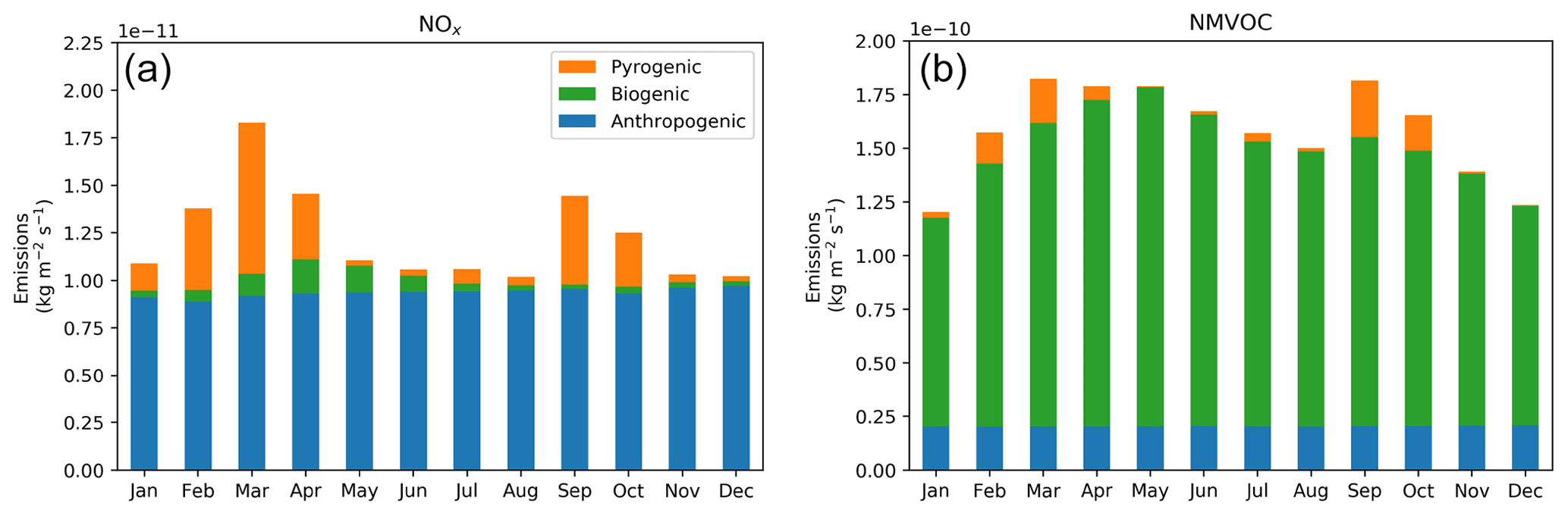
Figure 3Time series of monthly mean (a) NOx and (b) NMVOC emissions (kg m−2 s−1) from Southeast Asia in 2014. Emissions are sorted by source sector: anthropogenic, biogenic or pyrogenic. The source attribution for the full time series is extracted from the 2∘ × 2.5∘ global simulation.
The seasonal variation of NOx emissions, peaking in March and September, reflects the seasonal pattern of dry matter burning emissions as described above. During these two months, pyrogenic emissions of NOx account for 43 % and 32 % of total NOx emissions, respectively. Biogenic emissions of NOx, defined here as originating from soil only, also influence seasonal variations of NOx emissions over Southeast Asia but to a much lesser extent than burning. Biogenic emissions peak during April, accounting for only 12 % of total NOx emissions, and are lowest in August–January when the biogenic contribution does not exceed 3.54 × 10⁻¹³ kg m−2 s−1, or 3 % of the total. Anthropogenic activity represents the dominant source of NOx in Southeast Asia, accounting for more than 50 % of total NOx emissions in any given month. However, monthly anthropogenic emissions deviate no more than 5 % from the annual mean of 9.36 × 10⁻¹² kg m−2 s−1 and therefore have little impact on the seasonal trends of NOx emissions. Figure 4a–d shows that the spatial distributions of NOx emissions (kg m−2 s−1) during March and September are primarily determined by the pyrogenic sector, with a large but approximately constant anthropogenic influence discernible over major cities and ship tracks.
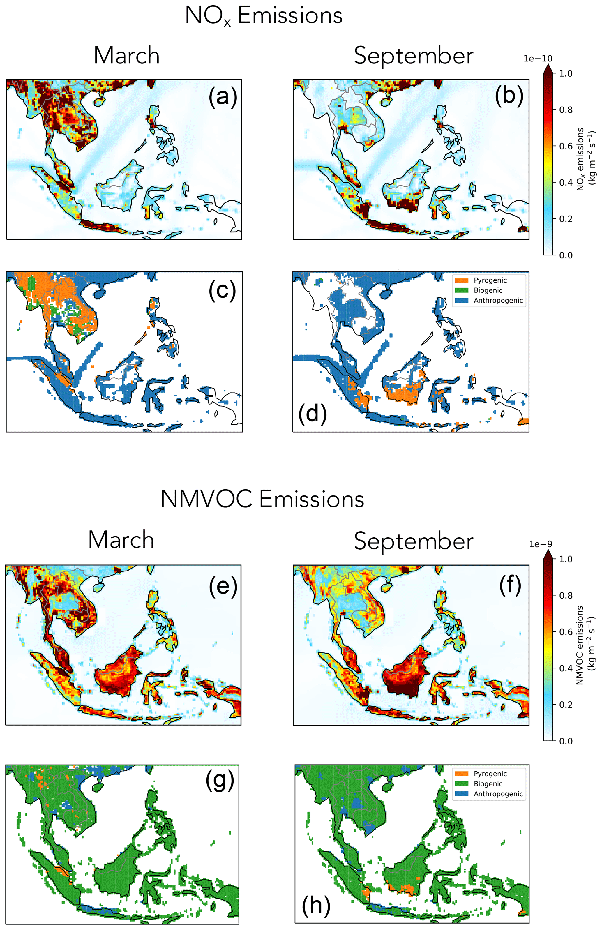
Figure 4Monthly mean emissions (kg m−2 s−1) of NOx and NMVOCs across Southeast Asia in March and September 2014. (a, b, e, f) Spatial distribution of emissions. (c, d, g, h) Map of the predominant emission source types: anthropogenic, biogenic or pyrogenic.
In contrast to NOx from Southeast Asia, seasonal emissions of NMVOCs are dominated by biogenic activity due mainly to isoprene. Monthly mean NMVOC emissions range from 1.20 × 10⁻¹⁰ to 1.82 × 10⁻¹⁰ kg m−2 s−1, with biogenic sources consistently accounting for more than 74 % of monthly emissions. Biogenic emissions have a strong seasonal pattern that peaks in May and September during the two regional dry seasons. Pyrogenic NMVOC emissions are comparatively much smaller in magnitude, accounting for 11 % and 15 % of total NMVOC emissions at their maximum values in March and September, respectively. However, they are still large enough to impact the seasonal trend of total NMVOC emissions, contributing to the domain-wide seasonal maximum in March. Despite lower biomass burning emissions overall, more pyrogenic NMVOC emissions are emitted in September due to the high fraction of organic carbon contained in peat soils (Kumar et al., 2020). Anthropogenic sources contribute only 13 % to total monthly mean NMVOC emissions and do not influence their seasonal variations. Figure 4e–h show that the spatial distributions of NMVOC emissions (kg m−2 s−1) in March and September are largely determined by the biogenic sector, with the highest emissions originating from rural areas that are predominantly plantations, farming and rainforest canopy. However, total NMVOC emissions may also be enhanced by spatial overlaps with anthropogenic and pyrogenic sources.
3.3 Seasonal changes in tropospheric ozone
Figure 5 shows monthly mean GEOS-Chem model and OMI measurements of tropospheric ozone columns (molec. cm−2) from 2014 averaged across Southeast Asia. The error bars shown for OMI are the standard errors in the mean as an indication of random error. Also shown are OMI values adjusted for bias estimates with respect to an ozonesonde ensemble as an indication of the systematic error range.1 Averaging kernels from OMI are applied to profiles from GEOS-Chem in order to produce comparable tropospheric ozone columns (Sect. 2.3).

Figure 5Time series of GEOS-Chem model and OMI monthly mean tropospheric ozone column (molec. cm−2) across Southeast Asia in 2014. Model results for the full time series are from the 2∘ × 2.5∘ global simulation. Error bars shown for OMI are the standard errors in the mean as an indication of random error. Also shown are OMI values adjusted for bias estimates with respect to an ozonesonde ensemble as an indication of the systematic error range.
Model tropospheric ozone over Southeast Asia peaks first during March, consistent with precursor emissions of NOx and NMVOC emissions (Fig. 3), with a value of 4.17 × 10¹⁷ molec. cm−2. The second model peak does not occur until October, which we find is due to a large positive flux from atmospheric transport into the region compared with the preceding month (Fig. 6). Minima in model tropospheric ozone occur during August and December, consistent with variations in the precursor emissions. Using the monthly mean tropospheric ozone columns from Fig. 5, we calculate that GEOS-Chem has a mean annual bias of −11 % compared to OMI (up to −30 % when OMI is adjusted for systematic error). The closest agreement occurs during March when the model has a positive bias of 7 % (−27 %). Tropospheric ozone from OMI peaks in May with a value of 4.35 (+1.29) × 1017 molec. cm−2 and not again until October. The annual cycle minimum occurs in January, although there is also a minimum in July between the two seasonal peaks. Broadly speaking, the seasonal trends in tropospheric ozone from GEOS-Chem are consistent with the OMI observations.

Figure 6GEOS-Chem model mean tropospheric ozone mass fluxes (kg s−1) over Southeast Asia in September and October 2014 averaged on the 2∘ × 2.5∘ global model grid. Fluxes are computed within GEOS-Chem and represent the difference in the model column mass before and after each component is applied. The troposphere is defined in this simulation using the dynamic tropopause height from GEOS-FP, which may not precisely correspond to the tropospheric columns defined in Sect. 2.1.
Figure 7 shows that tropospheric ozone columns (molec. cm−2) from both GEOS-Chem and OMI are clearly elevated over areas of seasonal fire activity during March and September 2014. During March, tropospheric ozone columns increase with latitude, with model values peaking at 8 × 10¹⁷ molec. cm−2 over mainland Southeast Asia, where we have shown biomass burning emissions are largest for that time of year (Fig. 2b, d). We find that in March the model has a mean positive bias of 22 % over that part of the region. During September, the spatial distribution of tropospheric ozone shifts away from mainland Southeast Asia into Indonesia, again consistent with the seasonal distribution of biomass burning emissions. The model generally has a negative bias with columns rarely exceeding 6 × 10¹⁷ molec. cm−2, except for locations where there are emissions from biomass burning (Fig. 2c, e).

Figure 7Spatial distribution of (a, d) the GEOS-Chem model and (b, e) OMI monthly mean tropospheric ozone column (molec. cm−2) across Southeast Asia in March and September 2014. Panels (c) and (f) show the difference between GEOS-Chem and OMI for March and September, respectively. Ozone columns are shown on the 0.25∘ × 0.3125∘ nested grid and are represented by white space where OMI observations are not available.
As shown above, precursors of tropospheric ozone originate from anthropogenic, biogenic and pyrogenic sources. Here, we explore how these emissions influence ozone photochemistry over Southeast Asia using three different ozone sensitivity indicators: (1) the ozone production rate, (2) ozone sensitivity to NOx and VOCs, and (3) ozone formation potential. Figure 8 shows the spatial distributions of all three indicators across Southeast Asia in March and September 2014. We provide a discussion on these indicators in the following sections.
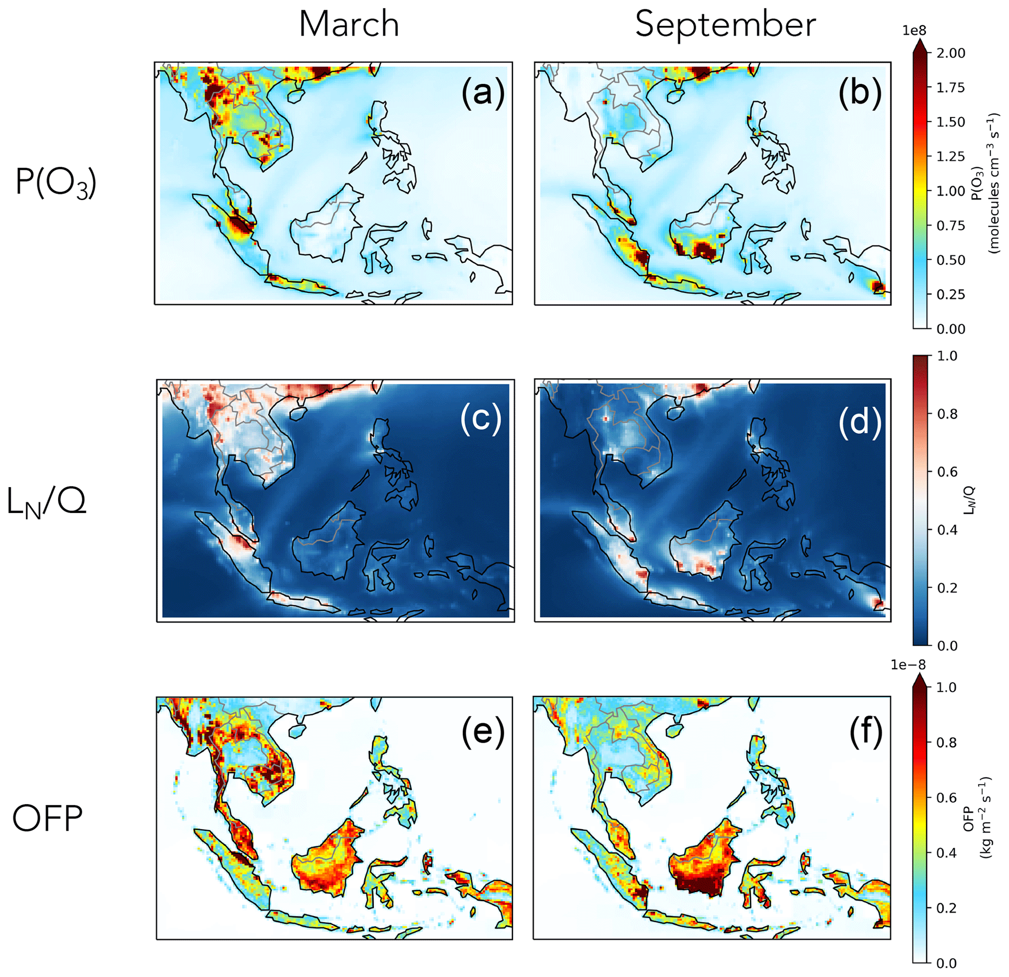
Figure 8Spatial distribution of model ozone sensitivity indicators across Southeast Asia in March and September 2014. (a, b) Mean ozone production rate (molec. cm−3 s−1) in the PBL during the daytime (06:00–18:00). (c, d) Mean in the PBL during the daytime (06:00–18:00). (e, f) Ozone formation potential (kg m−2 s−1).
4.1 Ozone production rates
Tropospheric ozone is produced when VOCs are oxidized in the presence of NOx. During the daytime, VOCs are oxidized by the hydroxyl radical (OH) to produce peroxy radicals (HO2 and RO2). In the presence of NOx, these peroxy radicals may react with NO to produce NO2, which photolyzes in sunlight to form atomic oxygen. Atomic oxygen and molecular oxygen then rapidly combine to produce ozone. The rate at which ozone is produced is limited by the conversion of NO to NO2 and is commonly represented as follows:
where P(O3) is the ozone production rate (molec. cm−3 s−1), and are rate constants corresponding to the subscripted reactions (cm3 molec.−1 s−1), and [HO2], [RO2i] and [NO] are species concentrations (molec. cm−3). The subscript i denotes that the second term is summed over multiple species of organic peroxy radicals. We use ozone production rates calculated by GEOS-Chem, which accounts for all contributing species as represented here by the complexSOA_SVPOA mechanism, including RO2 derived from isoprene, monoterpenes and smaller VOCs.
Figure 8a and b show GEOS-Chem ozone production rates (molec. cm−3 s−1) simulated over Southeast Asia during March and September 2014. We report the mean daytime value of P(O3) taken across the PBL to account for the influence of local mixing on surface air quality. Based on a qualitative comparison with Fig. 2, the highest ozone production rates, on the order of 2 × 10⁸ molec. cm−3 s−1, are largely co-located with fire emissions in both March and September. However, ozone production is also elevated over several major cities across the region where ozone production is dominated by the emission of precursors from the anthropogenic sector. Although the ozone production rate is useful in demonstrating the spatial correlation with biomass burning activity, it provides little insight into the mechanisms responsible for ozone production and the roles of ozone precursors in regional ozone photochemistry.
4.2 Ozone sensitivity to NOx and VOCs
Using GEOS-Chem model output, we calculate tropospheric ozone sensitivity to NOx and VOCs with the indicator, which represents the fraction of radical termination that results in the removal of NOx relative to HOx (HOx = OH + HO2) (Kleinman et al., 1997, 2001). Although both radical families are needed to form ozone, NOx is far less abundant than HOx, and the loss of NOx by radical termination effectively inhibits the production of ozone. The major terminal sinks for NOx and HOx are nitric acid (HNO3) and hydrogen peroxide (H2O2), respectively. Thus, the photochemical production rates for these species (molec. cm−3 s−1) are used to approximate radical termination in the calculation of :
Where , radical termination is mainly controlled by the loss of HOx, and ozone production varies linearly with NOx in a relationship that is considered NOx-limited. Where , ozone production is inhibited by the loss of NOx and becomes more sensitive to VOC emissions in a relationship that is considered VOC-limited. This method of calculating assumes a simplified removal scheme for HOx and NOx radicals, as both can also be removed through the formation of organic products. Loss of isoprene nitrates to hydrolysis has been shown to provide an important sink for NOx (Bates and Jacob, 2019). Although the organic sink for HOx may offset the impact of organic nitrates, formation of organic peroxides is intertwined with complex recycling mechanisms, which makes it difficult to assess the total impact of these uncertainties on our calculation of at this time.
Figure 8c and d show calculated from GEOS-Chem model output for March and September 2014. For consistency with the ozone production rates in Fig. 8a and b, we report mean daytime PBL values of . In general, we find that increases with NOx emissions and ozone production rates. The lowest values of occur where NOx emissions are low, even if VOC emissions are very high, such as over forests and croplands where there is no biomass burning activity. In these areas, is less than 0.5, indicating that ozone production is NOx-limited and therefore more sensitive to emissions of NOx than to VOC emissions. Values of tend to approach or exceed 0.5 over large cities and areas of biomass burning, indicating that these are instead characteristic of the VOC-limited regime. These areas coincide with the highest ozone production rates in Southeast Asia, suggesting that the majority of regional ozone forms under VOC-limited conditions. Although we cannot quantify sector-specific contributions to ozone production using , we can achieve this with our final ozone sensitivity indicator, the ozone formation potential.
4.3 Ozone formation potential
Ozone formation potential (OFP) is an ozone sensitivity indicator that relates ozone production directly to the emission of VOCs. To calculate OFP, we use the maximum incremental reactivity (MIR) scale developed by Carter (1994), whereby each emitted VOC is assigned a unique MIR that represents both the reactivity of that VOC to oxidation by OH and the capacity of that VOC once oxidized to produce ozone. The MIR scale is based on yields from the SAPRC photochemical mechanism (Carter, 1990) and has been validated in chamber studies (Carter, 1994, 1999, 2010). Here, we use the most recent MIR values provided by Carter (2010), which are described by grams of ozone formed per gram of VOC emitted. Because the MIR is a mass-based ratio, we simply multiply the emissions of each VOC (kg m−2 s−1) by its corresponding MIR to calculate OFP as a positive flux of ozone into the atmosphere (kg m−2 s−1):
We acknowledge that the MIR scale is derived by adjusting emissions of NOx to yield the highest possible incremental VOC reactivity. This means that OFP calculated from MIR assumes ozone production under VOC-limited conditions. Figure 8e and f show that OFP is generally enhanced over the parts of Southeast Asia that we have identified as VOC-limited. However, we calculate OFP for the entire region, which also includes many areas that may be NOx-limited. We do not filter OFP for VOC-limited conditions because precursor emissions and vary widely on much finer spatiotemporal scales than are represented here (Bai et al., 2015; Mazzuca et al., 2016; Van Der Werf et al., 2017). Thus, the assumption that OFP represents VOC-limited conditions introduces some uncertainties to our analysis, which we address in Sect. 4.4.
Different photochemical properties among source VOCs translate into a wide range of ozone formation capabilities. Table 1 shows VOCs with the highest assigned MIR that are emitted within GEOS-Chem. All of these species contain functional groups, such as alkenes and aldehydes, that are particularly reactive to oxidation by OH. Many of these are also large molecules containing multiple carbons that can be oxidized further to produce a high yield of ozone. When we apply MIR to NMVOC emission fluxes, we can determine which NMVOCs have the largest influence on OFP. Figure 9a shows the source attribution of OFP (kg m−2 s−1) to NMVOCs over Southeast Asia in March and September 2014. For both months, we find that the single largest contributor accounting for more than 60 % of OFP is isoprene (ISOP in GEOS-Chem), which is emitted in the model exclusively from biogenic sources. Other major contributors include propene (PRPE), acetaldehyde (ALD2), monoterpenes (MTPA and MTPO), formaldehyde (CH2O) and xylene (XYLE). Monoterpenes are primarily biogenic in origin, whereas many of the remaining NMVOCs are known products of biomass burning, especially from peat fires (Yokelson et al., 1997). Beyond these, other emitted NMVOCs account for less than 5 % of total OFP throughout the region.
Table 1Emitted VOCs in GEOS-Chem with the highest assigned MIR (grams of ozone formed per gram of VOC emitted). Adapted from Carter (2010).
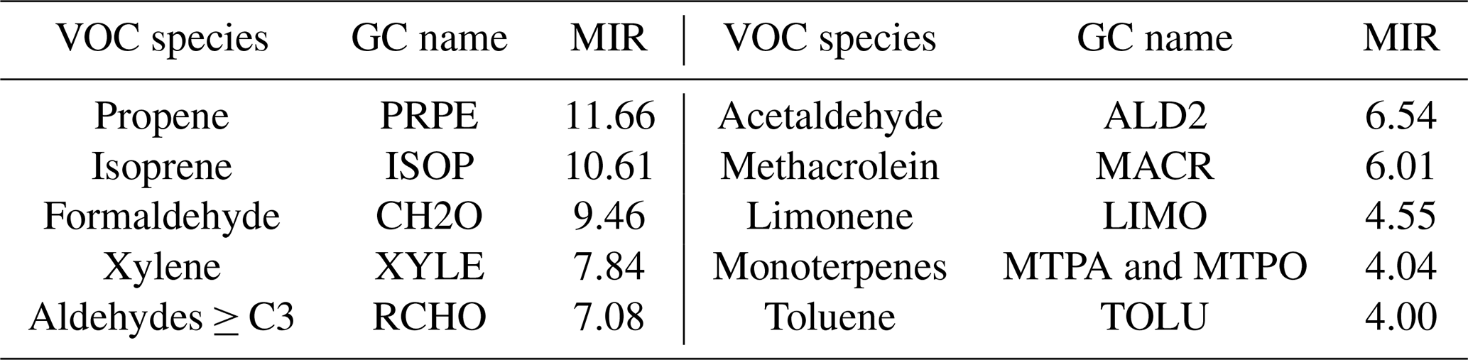
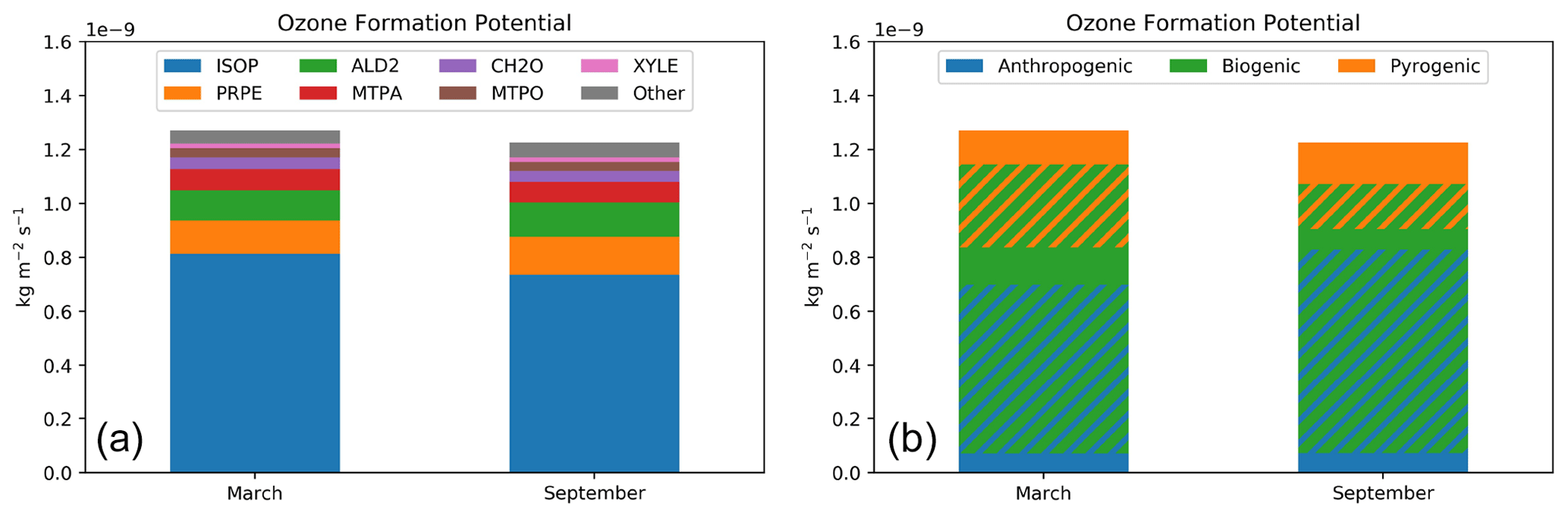
Figure 9Mean ozone formation potential (kg m−2 s−1) for Southeast Asia in March and September 2014 sorted by (a) individual species of emitted NMVOCs and (b) the source sector of emitted NMVOCs. Blue and orange hatching shows OFP from biogenic NMVOCs, scaled by the fraction of NOx emissions that are attributed to anthropogenic and pyrogenic sources, respectively.
We find that when OFP is sorted by the source sector of emitted NMVOCs, the majority of the OFP is attributed to biogenic NMVOCs, with only about 10 % and 5 % of the total OFP attributed to pyrogenic and anthropogenic NMVOCs, respectively. However, even under VOC-limited conditions, NOx is still required for VOC oxidation to result in the production of ozone. Therefore, other sources of NOx can still play a role in ozone formation, even when ozone-forming NMVOCs are mainly emitted from the biogenic sector. We estimate the overlap of biogenic NMVOCs with anthropogenic and pyrogenic NOx by scaling OFP in each grid cell by the fraction of total NOx emissions that are attributed to each sector. The results are represented by the blue and orange hatching in Fig. 9b. According to our estimates, overlap between biogenic NMVOCs and anthropogenic NOx makes the largest contribution to OFP, accounting for 49 % and 62 % of monthly mean OFP in March and September, respectively. The overlap of biogenic NMVOCs with pyrogenic NOx comprises the next largest source of ozone, accounting for up to 24 % of monthly mean OFP. With more than 90 % of OFP from pyrogenic NMVOCs attributed to the same source of NOx, we find overall that pyrogenic NOx accounts for 34 % of total OFP in March 2014 and 27 % in September over Southeast Asia.
4.4 Uncertainties
All the methods we use to interpret observed variations of tropospheric ozone are imperfect in some way. Here, we summarize some of the prominent uncertainties associated with these methods.
One of the largest uncertainties relevant to this work is the magnitude of biogenic NMVOC emissions. As mentioned in Sect. 2.3, the biogenic emissions model MEGAN2.1 has previously been shown to overestimate mean isoprene emissions in Southeast Asia by at least a factor of 2 (Langford et al., 2010; Stavrakou et al., 2014). Our model results suggest that the biogenic sector comprises a larger influence on OFP than any other NMVOC emission source and that isoprene is the single largest contributing NMVOC in Southeast Asia. Overestimation of biogenic NMVOCs in areas where ozone production is VOC-limited could explain the positive bias in the model tropospheric ozone columns, especially in March when biogenic emissions are higher over a larger portion of the region than they are in September. Overestimating biogenic emissions might also affect the relative contribution of pyrogenic NMVOCs to total OFP: if the biogenic contribution is substantially less, the fraction attributable to pyrogenic NMVOCs might be higher, although we acknowledge that pyrogenic emissions are equally as uncertain as biogenic emissions.
Emissions of NOx provide another potentially significant source of uncertainty. Pyrogenic emissions of NOx from GFED3.1 were previously shown to be biased low over Southeast Asia by as much as 45 % for the years 2005–2011 (Miyazaki et al., 2017). For the same time period, we find that GFED4.1s increases mean NOx emissions relative to GFED3 by 41 %, which largely corrects this bias. Some of our anthropogenic inventories, however, are out of date for 2014, including the MIX inventory for Asia, which is only available through 2010 (Li et al., 2017). Between 2010 and 2014, anthropogenic emissions are thought to have increased in Southeast Asia (Kurokawa and Ohara, 2020), implying that our model simulations may underestimate anthropogenic sources of NOx and NMVOCs. Although we do not expect that this would affect the seasonal variability in the anthropogenic emissions of either, our results suggest that the anthropogenic sector is a significant source of NOx, which could still impact regional ozone production. If emissions of NOx are underestimated from either anthropogenic or pyrogenic sources, ozone production could be higher and more VOC-limited than currently indicated by our results. This could also explain the negative bias in the model tropospheric ozone columns, especially towards the end of the year when the anthropogenic sector dominates the NOx emission distribution.
Our analysis is further limited by assumptions made in the derivation and application of OFP. As mentioned in Sect. 4.3, one of the major assumptions inherent in the calculation of OFP is that conditions for ozone production must be VOC-limited. We have shown using mean daytime from the PBL that ozone production is generally predicted to be VOC-limited over areas where ozone production is highest. However, we have calculated OFP across the region, which includes many areas that may be NOx-limited or near the transition between regimes. As a result, our estimate of OFP likely constitutes an upper limit on the yield of ozone from emitted NMVOCs and should not be compared directly with P(O3). Including areas that are not strictly VOC-limited may also inflate the influence of biogenic NMVOCs where NOx emissions are very low, for example over Borneo in March. As a sensitivity study, we recompute the sector-specific contributions to OFP after filtering by daytime PBL to exclude NOx-limited conditions. This filtering procedure increases the pyrogenic NMVOC contribution from about 10 % in March and September to 39 % and 63 %, respectively. Although the relative contribution from biogenic NMVOCs decreases overall, a larger fraction overlaps with pyrogenic NOx, increasing the total pyrogenic contribution from about 30 % to 80 % during both months. These values are much higher than those reported in Sect. 4.3 but also much more uncertain because we cannot be sure that our best estimate of precisely describes OFP, which is not similarly distributed throughout the atmosphere. Therefore, this treatment does not necessarily provide a better representation than is currently shown in Sect. 4.3, but it does suggest that our reported estimate of the fractional pyrogenic contribution to OFP may be too low, perhaps by as much as a factor of 2–3.
To assess the impact of regional ozone on public health, we use the maximum daily 8 h average (MDA8) metric, which sets the basis for public health guidelines around the world. To calculate MDA8, we construct an 8 h running mean of surface ozone concentrations and then select the maximum value from each 24 h day in local time. The World Health Organization (WHO) recommends a global limit on observed MDA8 ozone of 100 µg m−3 (≃50 ppbv) based on evidence that exposure to ozone at this level increases the number of attributable deaths by 1 %–2 % compared to a baseline of 70 µg m−3 (≃35 ppbv) (World Health Organization, 2006). Above the WHO recommended limit, the risk of mortality has been shown to increase with MDA8 ozone, even at short-term exposure timescales (Vicedo-Cabrera et al., 2020).
Mean MDA8 ozone exceeds the recommended exposure limit of 50 ppbv over a large fraction of Southeast Asia during both March and September 2014. Figure 10 presents maps of monthly mean MDA8 ozone (ppbv), as calculated from the GEOS-Chem nested model. Excessive values of MDA8 generally occur over areas of biomass burning and are widespread across the region due to the relatively long lifetime of ozone, which can be a few days at the surface in Southeast Asia. During March, prolonged exposure to ozone with MDA8 approaching 70 ppbv affects the majority of mainland Southeast Asia, home to 234 million people in 2014 (https://data.worldbank.org, last access: 17 December 2020). During September, excessive ozone persists over Indonesia, Southeast Asia's single most populous country, with a population of more than 255 million people at that time. As a basis for comparison, we also include maps of MDA8 ozone for May and December 2014, when emissions from biomass burning are at a minimum. During May, when biogenic emissions peak, MDA8 ozone approaches the WHO limit across the majority of the mainland but remains below 60 ppbv, and during December, MDA8 ozone is lower still and generally remains below 50 ppbv over land across the region. These results suggest that biomass burning coincides with the worst ozone air quality in the region, which exceeds WHO exposure guidelines.
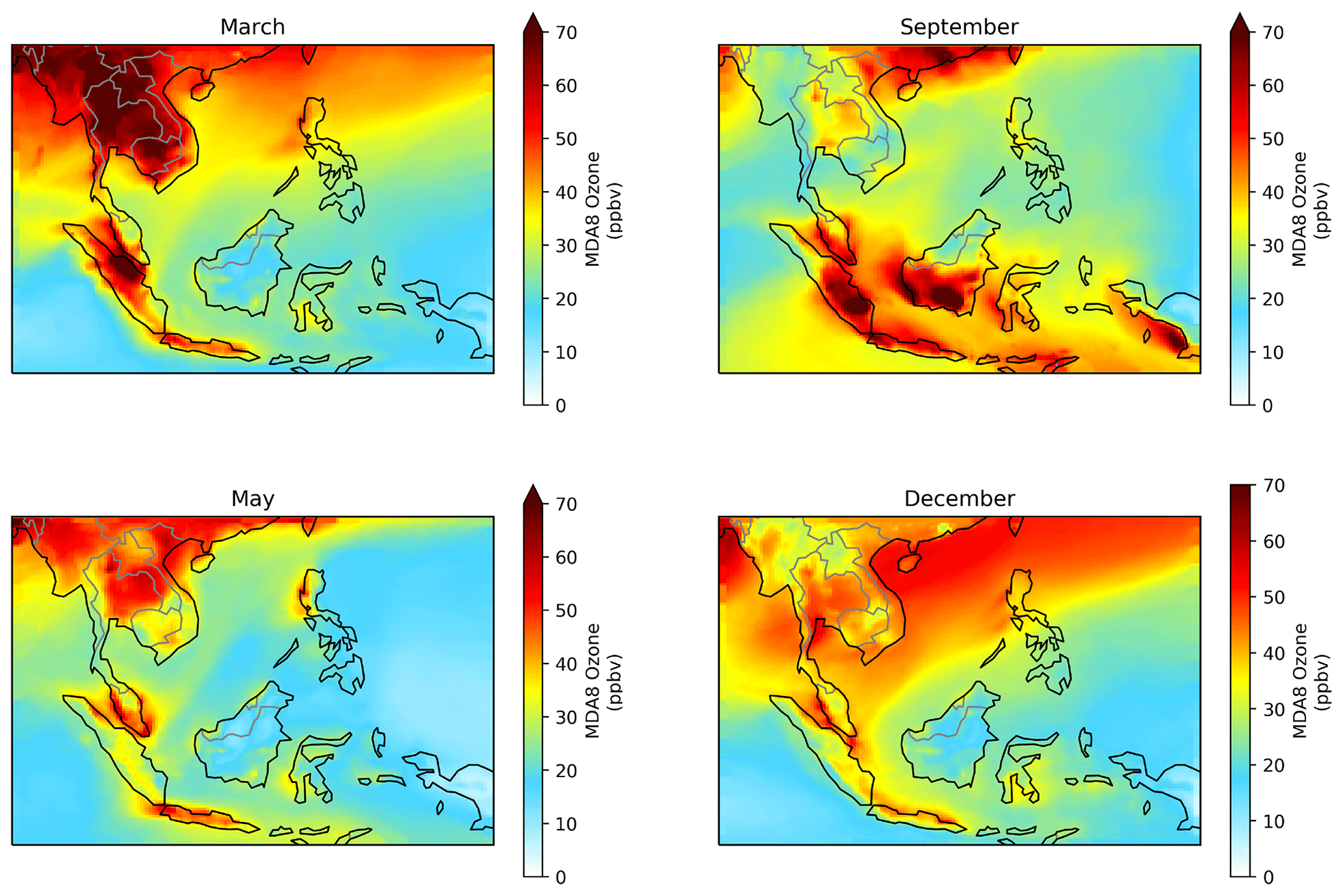
Figure 10Spatial distribution of monthly mean MDA8 ozone (ppbv) calculated for Southeast Asia in March, May, September and December 2014 based on surface concentrations of ozone from the GEOS-Chem nested model. For reference, the World Health Organization recommends an observed limit of ≃50 ppbv.
In a recent study, Vicedo-Cabrera et al. (2020) analyzed short-term ozone-related deaths across 406 cities in 20 countries between 1985 and 2015. They found that exposure to surface ozone at levels above the WHO guideline was associated with a 0.2 % mean increase in total short-term mortality. When we apply this factor to the gridded UN-adjusted population count product v4.11 for 2015 from the NASA Socioeconomic Data and Applications Center (https://sedac.ciesin.columbia.edu, last access: 17 December 2020), scaled to 2014 using national mortality and population data from the World Bank (https://data.worldbank.org, last access: 17 December 2020), we estimate that excessive ozone from biomass burning caused nearly 260 and 160 excess deaths across Southeast Asia in March and September, respectively. The mortality rate from Vicedo-Cabrera et al. (2020) varied substantially across the sampled countries and did not include any countries from Southeast Asia. Furthermore, their study did not account for interannual or seasonal variability, which we have shown exerts a large influence within our study domain. As a result, our estimate for the number of excess deaths in Southeast Asia is quite uncertain. However, our estimate is not unreasonable compared to Marlier et al. (2013), who estimated that severe fires in Indonesia pushed surface ozone concentrations above the WHO limit for 150 d in 1997, causing 4100 excess premature deaths. According to GFED4.1s fire emissions were more than 3 times higher in 1997 than they were in 2014, and they caused 2.5 times more exceedance days than are examined in this work. If the estimate from Marlier et al. (2013) is scaled for conditions in 2014, biomass burning should account for about 550 total ozone-attributed deaths during our study period, which agrees reasonably well with our estimate above.
We evaluate our GEOS-Chem values for MDA8 ozone using ground observations from Malaysia, which experiences reduced air quality during both regional burning seasons. As of 2020, the New Ambient Air Quality Standard (NAAQS) limits MDA8 ozone in Malaysia to 100 µg m−3, in line with WHO recommendations. The prior limit was set by the Malaysian Ambient Air Quality Guidelines (MAAQG), which restricted MDA8 ozone to 120 µg m−3 (60 ppbv) and had been in place since 1989 (DOE, 2015). Figure 11 shows model and observed monthly mean MDA8 ozone (ppbv) at ground site locations across Malaysia for March and September 2014. In March, the model predictions reproduce the observations reasonably well (r=0.82; slope = 0.78, y intercept = 12.79), with the highest values occurring along the western coast of peninsular Malaysia. This part of the country sits opposite the Riau province in Indonesia, which is a hot spot for fire emissions during the early burning season. The normalized mean bias (NMB) of the model, calculated as the mean difference between the model and observations normalized by the mean of the observations, is about 10 %. The model also accurately reproduces observed exceedances of monthly mean MDA8 ozone at 11 different ground sites relative to WHO guidelines, with two of these at the MAAQG level. However, the small positive model bias results in false MDA8 exceedances at another seven sites.
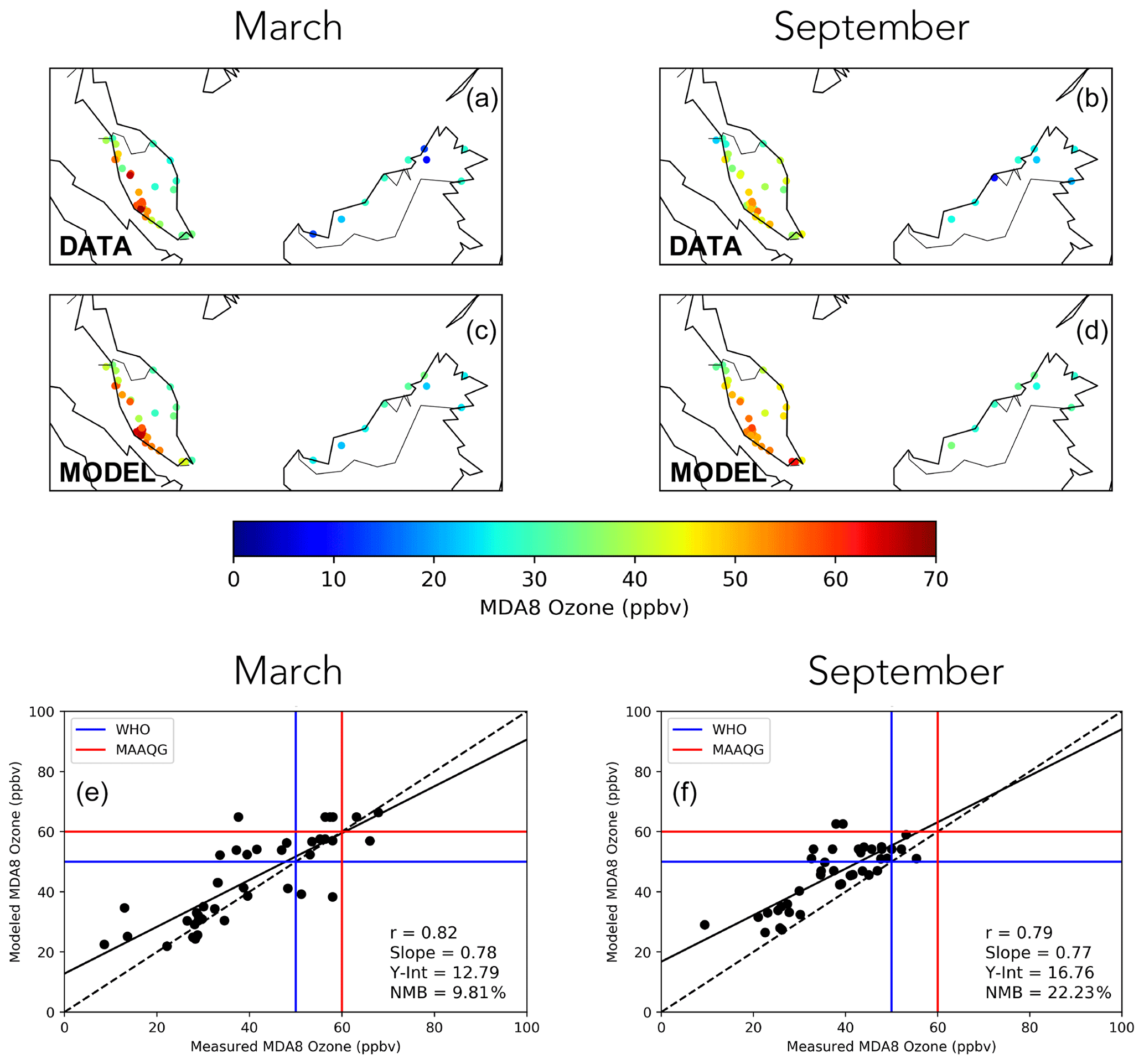
Figure 11Monthly mean MDA8 ozone (ppbv) across Malaysia in March and September 2014. (a–d) Observed and GEOS-Chem spatial distribution of MDA8 ozone at air quality monitoring sites. (e, f) Scatterplot of observed and GEOS-Chem MDA8 ozone at the air quality sites. A line of best fit is shown in black, with the associated mean statistics shown in the inset: Pearson correlation (r), the slope and y intercept of the best-fit line, and the normalized mean bias (NMB) as defined in the main text. Blue and red lines denote WHO and MAAQG MDA8 limits as of 2014.
Model performance is worse in September (r=0.79; slope = 0.77; y intercept = 16.76) when the NMB increases to 22 %. Model MDA8 ozone exceeds WHO guidelines at 17 ground sites, while only four of these are confirmed by observations. Although our analysis indicates that GEOS-Chem generally underestimates tropospheric ozone across Southeast Asia, the spatial distribution of the model bias shown in Figure 7f suggests that the model does overestimate tropospheric ozone over Malaysia in September, though the data coverage is insufficient to determine by how much. Although some ground sites are located near cities where anthropogenic sources may exert a larger influence on ozone production, we find that exceedances of monthly mean MDA8 are not confirmed by observations anywhere in Malaysia in either May or December when regional biomass burning is at a minimum. Despite a positive model bias, these results suggest that, although biogenic and anthropogenic ozone precursors may form the majority of MDA8 ozone across Southeast Asia, it is with the added influence from biomass burning that ozone exposure is elevated to hazardous levels exceeding global and national guidelines.
We used the GEOS-Chem atmospheric chemistry model, in combination with satellite and surface observations, to investigate the seasonal impacts of biomass burning on ozone air quality throughout Southeast Asia in 2014. Analysis of emission inventories emphasized two distinct biomass burning regimes: (1) burning on the peninsular mainland that peaks in March and (2) burning in Indonesia that peaks in September. Although the two burning seasons differ in the type of vegetation burned, both emit NOx and VOCs, which are ozone precursors. We found that outside burning areas, the underlying photochemical environment is generally NOx-limited and dominated by anthropogenic NOx and biogenic NMVOC emissions. Overall, however, pyrogenic NMVOCs are responsible for about 10 % of the regional OFP during both biomass burning seasons. Pyrogenic NOx is even more influential, shifting towards more VOC-limited ozone production and increasing the total pyrogenic contribution to about 30 % of OFP. Using model output, we showed that peak biomass burning activity coincides with widespread ozone exposure at levels that exceed world public health guidelines. We estimated that excess ozone from biomass burning caused about 260 premature deaths across Southeast Asia in March 2014 and another 160 deaths in September. Although the model tends to overestimate ozone near areas of biomass burning, surface observations confirm that hazardous ozone levels coincide with fire activity.
We found that model tropospheric ozone agrees relatively well with satellite (annual mean bias −11 %) and surface observations (r≥0.79, NMB ≤ 22.23 %), though some discrepancies remain unexplained. We suspect that these discrepancies are largely due to uncertainties associated with emission estimates. Biogenic emissions, for example, are calculated online in GEOS-Chem and may be overestimated in Southeast Asia by more than a factor of 2 (Langford et al., 2010; Stavrakou et al., 2014). The most recent inventory for anthropogenic emissions from Asia is from 2010, which is 4 years out of date with respect to 2014. Even biomass burning emissions, which are specified for 2014, vary greatly among the four inventories that are available for use within GEOS-Chem (Bauwens et al., 2016; Miyazaki et al., 2017). We also acknowledge that model uncertainties are not only limited to emission inventories, but may also be introduced through other components, including chemistry, mixing, deposition and transport (Travis et al., 2016; Eastham and Jacob, 2017; Marvin et al., 2017; Silva and Heald, 2018). Such uncertainties not only affect model ozone concentrations, but also the sensitivity of model ozone to its precursors and the influence of different source sectors. Development of effective air quality policy requires knowledge of how well these models describe surface air pollution and its driving processes.
Studies like ours would benefit immensely from further investigation into precursor emissions and the underlying chemical and physical processes that determine ozone across Southeast Asia. A regional network of ground-based remote sensing instruments for ozone and its precursors (e.g., Herman et al., 2009) would provide complementary measurements and serve as a useful validation source for satellite retrievals. Progress in spaceborne sensor technology has improved our ability to observe spatial scales associated with Southeast Asia. Improved temporal coverage will come from sensors aboard geostationary satellites that effectively hover over a particular geographical region. The South Korean Geostationary Environmental Satellite (GEMS), launched in February 2020, heralds the availability of multiple measurements of tropospheric ozone (Bak et al., 2013) and its precursors (Hong et al., 2017; Kwon et al., 2017) per day over Southeast Asia. Integration of these atmospheric data will ultimately require data assimilation or an inverse method framework (e.g., Miyazaki et al., 2020).
Model code and input data are free and available from the GEOS-Chem website (http://www.geos-chem.org, last access: 17 December 2020). Version 12.5.0 can be downloaded directly from https://doi.org/10.5281/zenodo.3403111 (The International GEOS-Chem User Community, 2019).
MRM and PIP designed experiments and wrote the paper. BGL, RS and BJK provided ozone retrieval data. MTL and MFK provided access to surface air quality data. All co-authors assisted in revising the paper.
The authors declare that they have no conflict of interest.
Many thanks to the Department of Environment, Ministry of Environment and Water, Malaysia, for providing surface air quality data. Production of OMI height-resolved data at Rutherford Appleton Laboratory was supported by the ESA's Climate Change Initiative.
This research has been supported by the Natural Environment Research Council through the National Centre for Earth Observation (grant nos. NE/R016518/1 and NE/R000115/1). Margaret R. Marvin, Paul I. Palmer, Barry G. Latter, Richard Siddans and Brian J. Kerridge were supported by grant number NE/R016518/1, with further support for Margaret R. Marvin from grant number NE/R000115/1.
This paper was edited by Bryan N. Duncan and reviewed by two anonymous referees.
Akagi, S. K., Yokelson, R. J., Wiedinmyer, C., Alvarado, M. J., Reid, J. S., Karl, T., Crounse, J. D., and Wennberg, P. O.: Emission factors for open and domestic biomass burning for use in atmospheric models, Atmos. Chem. Phys., 11, 4039–4072, https://doi.org/10.5194/acp-11-4039-2011, 2011. a
Bai, J., Guenther, A., Turnipseed, A., and Duhl, T.: Seasonal and interannual variations in whole-ecosystem isoprene and monoterpene emissions from a temperate mixed forest in Northern China, Atmos. Pollut. Res., 6, 696–707, https://doi.org/10.5094/APR.2015.078, 2015. a
Bak, J., Kim, J. H., Liu, X., Chance, K., and Kim, J.: Evaluation of ozone profile and tropospheric ozone retrievals from GEMS and OMI spectra, Atmos. Meas. Tech., 6, 239–249, https://doi.org/10.5194/amt-6-239-2013, 2013. a
Bates, K. H. and Jacob, D. J.: A new model mechanism for atmospheric oxidation of isoprene: global effects on oxidants, nitrogen oxides, organic products, and secondary organic aerosol, Atmos. Chem. Phys., 19, 9613–9640, https://doi.org/10.5194/acp-19-9613-2019, 2019. a
Bates, K. H., Crounse, J. D., St. Clair, J. M., Bennett, N. B., Nguyen, T. B., Seinfeld, J. H., Stoltz, B. M., and Wennberg, P. O.: Gas phase production and loss of isoprene epoxydiols, J. Phys. Chem. A, 118, 1237–1246, https://doi.org/10.1021/jp4107958, 2014. a
Bauwens, M., Stavrakou, T., Müller, J.-F., De Smedt, I., Van Roozendael, M., van der Werf, G. R., Wiedinmyer, C., Kaiser, J. W., Sindelarova, K., and Guenther, A.: Nine years of global hydrocarbon emissions based on source inversion of OMI formaldehyde observations, Atmos. Chem. Phys., 16, 10133–10158, https://doi.org/10.5194/acp-16-10133-2016, 2016. a
Bell, M. L., McDermott, A., Zeger, S. L., Samet, J. M., and Dominici, F.: Ozone and short-term mortality in 95 US urban communities, 1987–2000, JAMA, 292, 2372–8, https://doi.org/10.1001/jama.292.19.2372, 2004. a
Carter, W. P.: A detailed mechanism for the gas-phase atmospheric reactions of organic compounds, Atmos. Environ. Part A. Gen. Top., 24, 481–518, https://doi.org/10.1016/0960-1686(90)90005-8, 1990. a
Carter, W. P. L.: Development of ozone reactivity scales for volatile organic compounds, Air Waste, 44, 881–899, https://doi.org/10.1080/1073161X.1994.10467290, 1994. a, b
Carter, W. P. L.: Documentation of the SAPRC-99 chemical mechanism for VOC reactivity assessment, Tech. rep., California Air Resources Board, available at: https://intra.engr.ucr.edu/~carter/pubs/s99doc.pdf (last access: 17 December 2020), 1999. a
Carter, W. P. L.: Development of the SAPRC-07 chemical mechanism and updated ozone reactivity scales, Tech. rep., California Air Resources Board, https://intra.engr.ucr.edu/~carter/SAPRC/saprc07.pdf, last access: 17 December 2020), 2010. a, b, c
Chan Miller, C., Jacob, D. J., Marais, E. A., Yu, K., Travis, K. R., Kim, P. S., Fisher, J. A., Zhu, L., Wolfe, G. M., Hanisco, T. F., Keutsch, F. N., Kaiser, J., Min, K.-E., Brown, S. S., Washenfelder, R. A., González Abad, G., and Chance, K.: Glyoxal yield from isoprene oxidation and relation to formaldehyde: chemical mechanism, constraints from SENEX aircraft observations, and interpretation of OMI satellite data, Atmos. Chem. Phys., 17, 8725–8738, https://doi.org/10.5194/acp-17-8725-2017, 2017. a
Csiszar, I., Denis, L., Giglio, L., Justice, C. O., and Hewson, J.: Global fire activity from two years of MODIS data, Int. J. Wildl. Fire, 14, 117–130, https://doi.org/10.1071/WF03078, 2005. a
DOE: New Malaysia Ambient Air Quality Standard, Tech. Rep., Department of Environment, Ministry of Environment and Water of Malaysia, available at: http://www.doe.gov.my/portalv1/wp-content/uploads/2013/01/Air-Quality-Standard-BI.pdf (last access: 13 August 2020), 2015. a
Duncan, B. N., Martin, R. V., Staudt, A. C., Yevich, R., and Logan, J. A.: Interannual and seasonal variability of biomass burning emissions constrained by satellite observations, J. Geophys. Res., 108, 4100, https://doi.org/10.1029/2002JD002378, 2003. a
Eastham, S. D. and Jacob, D. J.: Limits on the ability of global Eulerian models to resolve intercontinental transport of chemical plumes, Atmos. Chem. Phys., 17, 2543–2553, https://doi.org/10.5194/acp-17-2543-2017, 2017. a
Eastham, S. D., Weisenstein, D. K., and Barrett, S. R.: Development and evaluation of the unified tropospheric–stratospheric chemistry extension (UCX) for the global chemistry-transport model GEOS-Chem, Atmos. Environ., 89, 52–63, https://doi.org/10.1016/J.ATMOSENV.2014.02.001, 2014. a
Field, R. D., van der Werf, G. R., Fanin, T., Fetzer, E. J., Fuller, R., Jethva, H., Levy, R., Livesey, N. J., Luo, M., Torres, O., and Worden, H. M.: Indonesian fire activity and smoke pollution in 2015 show persistent nonlinear sensitivity to El Niño-induced drought, Proc. Natl. Acad. Sci. USA, 113, 9204–9209, https://doi.org/10.1073/pnas.1524888113, 2016. a
Fisher, J. A., Jacob, D. J., Travis, K. R., Kim, P. S., Marais, E. A., Chan Miller, C., Yu, K., Zhu, L., Yantosca, R. M., Sulprizio, M. P., Mao, J., Wennberg, P. O., Crounse, J. D., Teng, A. P., Nguyen, T. B., St. Clair, J. M., Cohen, R. C., Romer, P., Nault, B. A., Wooldridge, P. J., Jimenez, J. L., Campuzano-Jost, P., Day, D. A., Hu, W., Shepson, P. B., Xiong, F., Blake, D. R., Goldstein, A. H., Misztal, P. K., Hanisco, T. F., Wolfe, G. M., Ryerson, T. B., Wisthaler, A., and Mikoviny, T.: Organic nitrate chemistry and its implications for nitrogen budgets in an isoprene- and monoterpene-rich atmosphere: constraints from aircraft (SEAC4RS) and ground-based (SOAS) observations in the Southeast US, Atmos. Chem. Phys., 16, 5969–5991, https://doi.org/10.5194/acp-16-5969-2016, 2016. a
Guenther, A. B., Jiang, X., Heald, C. L., Sakulyanontvittaya, T., Duhl, T., Emmons, L. K., and Wang, X.: The Model of Emissions of Gases and Aerosols from Nature version 2.1 (MEGAN2.1): an extended and updated framework for modeling biogenic emissions, Geosci. Model Dev., 5, 1471–1492, https://doi.org/10.5194/gmd-5-1471-2012, 2012. a, b
Herawati, H. and Santoso, H.: Tropical forest susceptibility to and risk of fire under changing climate: A review of fire nature, policy and institutions in Indonesia, For. Policy Econ., 13, 227–233, https://doi.org/10.1016/J.FORPOL.2011.02.006, 2011. a
Herman, J., Cede, A., Spinei, E., Mount, G., Tzortziou, M., and Abuhassan, N.: NO2 column amounts from ground-based Pandora and MFDOAS spectrometers using the direct-sun DOAS technique: Intercomparisons and application to OMI validation, J. Geophys. Res.-Atmos., 114, D13307, https://doi.org/10.1029/2009JD011848, 2009. a
Hoesly, R. M., Smith, S. J., Feng, L., Klimont, Z., Janssens-Maenhout, G., Pitkanen, T., Seibert, J. J., Vu, L., Andres, R. J., Bolt, R. M., Bond, T. C., Dawidowski, L., Kholod, N., Kurokawa, J.-I., Li, M., Liu, L., Lu, Z., Moura, M. C. P., O'Rourke, P. R., and Zhang, Q.: Historical (1750–2014) anthropogenic emissions of reactive gases and aerosols from the Community Emissions Data System (CEDS), Geosci. Model Dev., 11, 369–408, https://doi.org/10.5194/gmd-11-369-2018, 2018. a, b
Hong, H., Lee, H., Kim, J., Jeong, U., Ryu, J., and Lee, D. S.: Investigation of simultaneous effects of aerosol properties and aerosol peak height on the air mass factors for space-borne NO2 retrievals, Remote Sens., 9, 208, https://doi.org/10.3390/rs9030208, 2017. a
Hudman, R. C., Moore, N. E., Mebust, A. K., Martin, R. V., Russell, A. R., Valin, L. C., and Cohen, R. C.: Steps towards a mechanistic model of global soil nitric oxide emissions: implementation and space based-constraints, Atmos. Chem. Phys., 12, 7779–7795, https://doi.org/10.5194/acp-12-7779-2012, 2012. a
Huijnen, V., Wooster, M. J., Kaiser, J. W., Gaveau, D. L. A., Flemming, J., Parrington, M., Inness, A., Murdiyarso, D., Main, B., and van Weele, M.: Fire carbon emissions over maritime southeast Asia in 2015 largest since 1997, Sci. Rep.-UK, 6, 26886, https://doi.org/10.1038/srep26886, 2016. a
Jacob, D. J.: Introduction to Atmospheric Chemistry, Princeton University Press, Princeton, USA, 1999. a
Jones, D.: ASEAN and transboundary haze pollution in Southeast Asia, Asia Eur. J., 4, 431–446, https://doi.org/10.1007/s10308-006-0067-1, 2006. a
Kita, K., Fujiwara, M., and Kawakami, S.: Total ozone increase associated with forest fires over the Indonesian region and its relation to the El Niño-Southern oscillation, Atmos. Environ., 34, 2681–2690, https://doi.org/10.1016/S1352-2310(99)00522-1, 2000. a
Kleinman, L. I., Daum, P. H., Lee, J. H., Lee, Y.-N., Nunnermacker, L. J., Springston, S. R., Newman, L., Weinstein-Lloyd, J., and Sillman, S.: Dependence of ozone production on NO and hydrocarbons in the troposphere, Geophys. Res. Lett., 24, 2299–2302, https://doi.org/10.1029/97GL02279, 1997. a
Kleinman, L. I., Daum, P. H., Lee, Y.-N., Nunnermacker, L. J., Springston, S. R., Weinstein-Lloyd, J., and Rudolph, J.: Sensitivity of ozone production rate to ozone precursors, Geophys. Res. Lett., 28, 2903–2906, https://doi.org/10.1029/2000GL012597, 2001. a
Korontzi, S., McCarty, J., Loboda, T., Kumar, S., and Justice, C.: Global distribution of agricultural fires in croplands from 3 years of Moderate Resolution Imaging Spectroradiometer (MODIS) data, Global Biogeochem. Cy., 20, GB2021, https://doi.org/10.1029/2005GB002529, 2006. a
Kumar, P., Adelodun, A. A., Khan, M. F., Krisnawati, H., and Garcia-Menendez, F.: Towards an improved understanding of greenhouse gas emissions and fluxes in tropical peatlands of Southeast Asia, Sustain. Cities Soc., 53, 101881, https://doi.org/10.1016/j.scs.2019.101881, 2020. a
Kurokawa, J. and Ohara, T.: Long-term historical trends in air pollutant emissions in Asia: Regional Emission inventory in ASia (REAS) version 3, Atmos. Chem. Phys., 20, 12761–12793, https://doi.org/10.5194/acp-20-12761-2020, 2020. a
Kwon, H.-A., Park, R. J., Jeong, J. I., Lee, S., González Abad, G., Kurosu, T. P., Palmer, P. I., and Chance, K.: Sensitivity of formaldehyde (HCHO) column measurements from a geostationary satellite to temporal variation of the air mass factor in East Asia, Atmos. Chem. Phys., 17, 4673–4686, https://doi.org/10.5194/acp-17-4673-2017, 2017. a
Langford, B., Misztal, P. K., Nemitz, E., Davison, B., Helfter, C., Pugh, T. A. M., MacKenzie, A. R., Lim, S. F., and Hewitt, C. N.: Fluxes and concentrations of volatile organic compounds from a South-East Asian tropical rainforest, Atmos. Chem. Phys., 10, 8391–8412, https://doi.org/10.5194/acp-10-8391-2010, 2010. a, b, c
Latif, M. T., Dominick, D., Ahamad, F., Khan, M. F., Juneng, L., Hamzah, F. M., and Nadzir, M. S. M.: Long term assessment of air quality from a background station on the Malaysian Peninsula, Sci. Total Environ., 482–483, 336–348, https://doi.org/10.1016/J.SCITOTENV.2014.02.132, 2014. a
Lee, L., Teng, A. P., Wennberg, P. O., Crounse, J. D., and Cohen, R. C.: On rates and mechanisms of OH and O3 reactions with isoprene-derived hydroxy nitrates, J. Phys. Chem. A, 118, 1622–1637, https://doi.org/10.1021/jp4107603, 2014. a
Levelt, P. F., Van Den Oord, G. H. J., Dobber, M. R., Mälkki, A., Visser, H., De Vries, J., Stammes, P., Lundell, J. O. V., and Saari, H.: The Ozone Monitoring Instrument, IEEE T. Geosci. Remote, 44, 1093, https://doi.org/10.1109/TGRS.2006.872333, 2006. a
Levelt, P. F., Joiner, J., Tamminen, J., Veefkind, J. P., Bhartia, P. K., Stein Zweers, D. C., Duncan, B. N., Streets, D. G., Eskes, H., van der A, R., McLinden, C., Fioletov, V., Carn, S., de Laat, J., DeLand, M., Marchenko, S., McPeters, R., Ziemke, J., Fu, D., Liu, X., Pickering, K., Apituley, A., González Abad, G., Arola, A., Boersma, F., Chan Miller, C., Chance, K., de Graaf, M., Hakkarainen, J., Hassinen, S., Ialongo, I., Kleipool, Q., Krotkov, N., Li, C., Lamsal, L., Newman, P., Nowlan, C., Suleiman, R., Tilstra, L. G., Torres, O., Wang, H., and Wargan, K.: The Ozone Monitoring Instrument: overview of 14 years in space, Atmos. Chem. Phys., 18, 5699–5745, https://doi.org/10.5194/acp-18-5699-2018, 2018. a
Li, M., Zhang, Q., Kurokawa, J.-I., Woo, J.-H., He, K., Lu, Z., Ohara, T., Song, Y., Streets, D. G., Carmichael, G. R., Cheng, Y., Hong, C., Huo, H., Jiang, X., Kang, S., Liu, F., Su, H., and Zheng, B.: MIX: a mosaic Asian anthropogenic emission inventory under the international collaboration framework of the MICS-Asia and HTAP, Atmos. Chem. Phys., 17, 935–963, https://doi.org/10.5194/acp-17-935-2017, 2017. a, b, c
Marais, E. A., Jacob, D. J., Jimenez, J. L., Campuzano-Jost, P., Day, D. A., Hu, W., Krechmer, J., Zhu, L., Kim, P. S., Miller, C. C., Fisher, J. A., Travis, K., Yu, K., Hanisco, T. F., Wolfe, G. M., Arkinson, H. L., Pye, H. O. T., Froyd, K. D., Liao, J., and McNeill, V. F.: Aqueous-phase mechanism for secondary organic aerosol formation from isoprene: application to the southeast United States and co-benefit of SO2 emission controls, Atmos. Chem. Phys., 16, 1603–1618, https://doi.org/10.5194/acp-16-1603-2016, 2016. a, b
Marlier, M. E., DeFries, R. S., Voulgarakis, A., Kinney, P. L., Randerson, J. T., Shindell, D. T., Chen, Y., and Faluvegi, G.: El Niño and health risks from landscape fire emissions in Southeast Asia, Nat. Clim. Change, 3, 131–136, https://doi.org/10.1038/nclimate1658, 2013. a, b, c
Marlier, M. E., DeFries, R. S., Kim, P. S., Koplitz, S. N., Jacob, D. J., Mickley, L. J., and Myers, S. S.: Fire emissions and regional air quality impacts from fires in oil palm, timber, and logging concessions in Indonesia, Environ. Res. Lett., 10, 85005, https://doi.org/10.1088/1748-9326/10/8/085005, 2015. a
Marvin, M. R., Wolfe, G. M., Salawitch, R. J., Canty, T. P., Roberts, S. J., Travis, K. R., Aikin, K. C., de Gouw, J. A., Graus, M., Hanisco, T. F., Holloway, J. S., Hübler, G., Kaiser, J., Keutsch, F. N., Peischl, J., Pollack, I. B., Roberts, J. M., Ryerson, T. B., Veres, P. R., and Warneke, C.: Impact of evolving isoprene mechanisms on simulated formaldehyde: An inter-comparison supported by in situ observations from SENEX, Atmos. Environ., 164, 325–336, https://doi.org/10.1016/J.ATMOSENV.2017.05.049, 2017. a, b
Mazzuca, G. M., Ren, X., Loughner, C. P., Estes, M., Crawford, J. H., Pickering, K. E., Weinheimer, A. J., and Dickerson, R. R.: Ozone production and its sensitivity to NOx and VOCs: results from the DISCOVER-AQ field experiment, Houston 2013, Atmos. Chem. Phys., 16, 14463–14474, https://doi.org/10.5194/acp-16-14463-2016, 2016. a
Miles, G. M., Siddans, R., Kerridge, B. J., Latter, B. G., and Richards, N. A. D.: Tropospheric ozone and ozone profiles retrieved from GOME-2 and their validation, Atmos. Meas. Tech., 8, 385–398, https://doi.org/10.5194/amt-8-385-2015, 2015. a, b
Miyazaki, K., Eskes, H., Sudo, K., Boersma, K. F., Bowman, K., and Kanaya, Y.: Decadal changes in global surface NOx emissions from multi-constituent satellite data assimilation, Atmos. Chem. Phys., 17, 807–837, https://doi.org/10.5194/acp-17-807-2017, 2017. a, b
Miyazaki, K., Bowman, K. W., Yumimoto, K., Walker, T., and Sudo, K.: Evaluation of a multi-model, multi-constituent assimilation framework for tropospheric chemical reanalysis, Atmos. Chem. Phys., 20, 931–967, https://doi.org/10.5194/acp-20-931-2020, 2020. a
Müller, J.-F., Peeters, J., and Stavrakou, T.: Fast photolysis of carbonyl nitrates from isoprene, Atmos. Chem. Phys., 14, 2497–2508, https://doi.org/10.5194/acp-14-2497-2014, 2014. a
Murray, L. T., Jacob, D. J., Logan, J. A., Hudman, R. C., and Koshak, W. J.: Optimized regional and interannual variability of lightning in a global chemical transport model constrained by LIS/OTD satellite data, J. Geophys. Res.-Atmos., 117, D20307, https://doi.org/10.1029/2012JD017934, 2012. a
Pochanart, P., Kreasuwun, J., Sukasem, P., Geeratithadaniyom, W., Tabucanon, M. S., Hirokawa, J., Kajii, Y., and Akimoto, H.: Tropical tropospheric ozone observed in Thailand, Atmos. Environ., 35, 2657–2668, https://doi.org/10.1016/S1352-2310(00)00441-6, 2001. a
Pye, H. O. T., Chan, A. W. H., Barkley, M. P., and Seinfeld, J. H.: Global modeling of organic aerosol: the importance of reactive nitrogen (NOx and NO3), Atmos. Chem. Phys., 10, 11261–11276, https://doi.org/10.5194/acp-10-11261-2010, 2010. a
Samet, J. M., Dominici, F., Curriero, F. C., Coursac, I., and Zeger, S. L.: Fine particulate air pollution and mortality in 20 U.S. cities, 1987–1994, N. Engl. J. Med., 343, 1742–1749, https://doi.org/10.1056/NEJM200012143432401, 2000. a
Sastry, N.: Forest fires, air pollution, and mortality in Southeast Asia, Demography, 39, 1–23, https://doi.org/10.1353/dem.2002.0009, 2002. a
Sillman, S.: The relation between ozone, NOx and hydrocarbons in urban and polluted rural environments, Atmos. Environ., 33, 1821–1845, https://doi.org/10.1016/S1352-2310(98)00345-8, 1999. a
Sillman, S., Logan, J. A., and Wofsy, S. C.: The sensitivity of ozone to nitrogen oxides and hydrocarbons in regional ozone episodes, J. Geophys. Res., 95, 1837, https://doi.org/10.1029/JD095iD02p01837, 1990. a
Silva, S. J. and Heald, C. L.: Investigating dry deposition of ozone to vegetation, J. Geophys. Res.-Atmos., 123, 559–573, https://doi.org/10.1002/2017JD027278, 2018. a
Stavrakou, T., Müller, J.-F., Bauwens, M., De Smedt, I., Van Roozendael, M., Guenther, A., Wild, M., and Xia, X.: Isoprene emissions over Asia 1979–2012: impact of climate and land-use changes, Atmos. Chem. Phys., 14, 4587–4605, https://doi.org/10.5194/acp-14-4587-2014, 2014. a, b, c
Stettler, M. E. J., Eastham, S., and Barrett, S. R. H.: Air quality and public health impacts of UK airports. Part I: Emissions, Atmos. Environ., 45, 5415–5424, https://doi.org/10.1016/j.atmosenv.2011.07.012, 2011. a, b
The International GEOS-Chem User Community: geoschem/geos-chem: GEOS-Chem 12.5.0 (Version 12.5.0), Zenodo, https://doi.org/10.5281/zenodo.3403111, 2019. a
Thompson, A. M., Witte, J. C., Hudson, R. D., Guo, H., Herman, J. R., and Fujiwara, M.: Tropical tropospheric ozone and biomass burning, Science, 291, 2128–2132, https://doi.org/10.1126/science.291.5511.2128, 2001. a
Thornton, J. A., Wooldridge, P. J., Cohen, R. C., Martinez, M., Harder, H., Brune, W. H., Williams, E. J., Roberts, J. M., Fehsenfeld, F. C., Hall, S. R., Shetter, R. E., Wert, B. P., and Fried, A.: Ozone production rates as a function of NOx abundances and HOx production rates in the Nashville urban plume, J. Geophys. Res., 107, 4146, https://doi.org/10.1029/2001JD000932, 2002. a
Toh, Y. Y., Lim, S. F., and von Glasow, R.: The influence of meteorological factors and biomass burning on surface ozone concentrations at Tanah Rata, Malaysia, Atmos. Environ., 70, 435–446, https://doi.org/10.1016/J.ATMOSENV.2013.01.018, 2013. a
Trainer, M., Williams, E. J., Parrish, D. D., Buhr, M. P., Allwine, E. J., Westberg, H. H., Fehsenfeld, F. C., and Liu, S. C.: Models and observations of the impact of natural hydrocarbons on rural ozone, Nature, 329, 705–707, https://doi.org/10.1038/329705a0, 1987. a
Travis, K. R., Jacob, D. J., Fisher, J. A., Kim, P. S., Marais, E. A., Zhu, L., Yu, K., Miller, C. C., Yantosca, R. M., Sulprizio, M. P., Thompson, A. M., Wennberg, P. O., Crounse, J. D., St. Clair, J. M., Cohen, R. C., Laughner, J. L., Dibb, J. E., Hall, S. R., Ullmann, K., Wolfe, G. M., Pollack, I. B., Peischl, J., Neuman, J. A., and Zhou, X.: Why do models overestimate surface ozone in the Southeast United States?, Atmos. Chem. Phys., 16, 13561–13577, https://doi.org/10.5194/acp-16-13561-2016, 2016. a, b
Vadrevu, K. P., Lasko, K., Giglio, L., Schroeder, W., Biswas, S., and Justice, C.: Trends in vegetation fires in South and Southeast Asian countries, Sci. Rep.-UK, 9, 7422, https://doi.org/10.1038/s41598-019-43940-x, 2019. a
van der Werf, G. R., Dempewolf, J., Trigg, S. N., Randerson, J. T., Kasibhatla, P. S., Giglio, L., Murdiyarso, D., Peters, W., Morton, D. C., Collatz, G. J., Dolman, A. J., and DeFries, R. S.: Climate regulation of fire emissions and deforestation in equatorial Asia, P. Natl. Acad. Sci. USA, 105, 20350–20355, https://doi.org/10.1073/pnas.0803375105, 2008. a
van der Werf, G. R., Randerson, J. T., Giglio, L., van Leeuwen, T. T., Chen, Y., Rogers, B. M., Mu, M., van Marle, M. J. E., Morton, D. C., Collatz, G. J., Yokelson, R. J., and Kasibhatla, P. S.: Global fire emissions estimates during 1997–2016, Earth Syst. Sci. Data, 9, 697–720, https://doi.org/10.5194/essd-9-697-2017, 2017. a, b
Vicedo-Cabrera, A. M., Sera, F., Liu, C., Armstrong, B., Milojevic, A., Guo, Y., Tong, S., Lavigne, E., Kyselý, J., Urban, A., Orru, H., Indermitte, E., Pascal, M., Huber, V., Schneider, A., Katsouyanni, K., Samoli, E., Stafoggia, M., Scortichini, M., Hashizume, M., Honda, Y., Ng, C. F. S., Hurtado-Diaz, M., Cruz, J., Silva, S., Madureira, J., Scovronick, N., Garland, R. M., Kim, H., Tobias, A., Íñiguez, C., Forsberg, B., Åström, C., Ragettli, M. S., Röösli, M., Guo, Y.-L. L., Chen, B.-Y., Zanobetti, A., Schwartz, J., Bell, M. L., Kan, H., and Gasparrini, A.: Short term association between ozone and mortality: Global two stage time series study in 406 locations in 20 countries, BMJ, 368, m108, https://doi.org/10.1136/bmj.m108, 2020. a, b, c, d
Wooster, M. J., Perry, G. L. W., and Zoumas, A.: Fire, drought and El Niño relationships on Borneo (Southeast Asia) in the pre-MODIS era (1980–2000), Biogeosciences, 9, 317–340, https://doi.org/10.5194/bg-9-317-2012, 2012. a
World Health Organization: WHO Air quality guidelines for particulate matter, ozone, nitrogen dioxide and sulfur dioxide: Global update 2005: Summary of risk assessment, available at: https://apps.who.int/iris/bitstream/handle/10665/69477/WHO_SDE_PHE_OEH_06.02_eng.pdf (last access: 2 February 2021), World Health Organization, 2006. a
Xie, Y., Paulot, F., Carter, W. P. L., Nolte, C. G., Luecken, D. J., Hutzell, W. T., Wennberg, P. O., Cohen, R. C., and Pinder, R. W.: Understanding the impact of recent advances in isoprene photooxidation on simulations of regional air quality, Atmos. Chem. Phys., 13, 8439–8455, https://doi.org/10.5194/acp-13-8439-2013, 2013. a
Yokelson, R. J., Susott, R., Ward, D. E., Reardon, J., and Griffith, D. W. T.: Emissions from smoldering combustion of biomass measured by open-path Fourier transform infrared spectroscopy, J. Geophys. Res.-Atmos., 102, 18865–18877, https://doi.org/10.1029/97JD00852, 1997. a
Ziemke, J. R., Chandra, S., Duncan, B. N., Schoeberl, M. R., Torres, O., Damon, M. R., and Bhartia, P. K.: Recent biomass burning in the tropics and related changes in tropospheric ozone, Geophys. Res. Lett., 36, L15819, https://doi.org/10.1029/2009GL039303, 2009. a
Bias with respect to ozonesondes is derived as a function of latitude and month of year by applying averaging kernels from individual soundings to sonde profiles and averaging over all processed years of the OMI mission. It should be noted, however, that ozonesonde stations are sparse in the latitude range used for this study, particularly in the Southeast Asia longitude sector.
- Abstract
- Introduction
- Data and methods
- Results
- How do biomass burning emissions impact variations in tropospheric ozone?
- Implications for public health
- Concluding remarks
- Code and data availability
- Author contributions
- Competing interests
- Acknowledgements
- Financial support
- Review statement
- References