the Creative Commons Attribution 4.0 License.
the Creative Commons Attribution 4.0 License.
 | 21 Dec 2021
A simple model of ozone–temperature coupling in the tropical lower stratosphere
Fei Wu
Alison Ming
Peter Hitchcock
Observations show strong correlations between large-scale ozone and temperature variations in the tropical lower stratosphere across a wide range of timescales. We quantify this behavior using monthly records of ozone and temperature data from Southern Hemisphere Additional Ozonesonde (SHADOZ) tropical balloon measurements (1998–2016), along with global satellite data from Aura microwave limb sounder and GPS radio occultation over 2004–2018. The observational data demonstrate strong in-phase ozone–temperature coherence spanning sub-seasonal, annual and interannual timescales, and the slope of the temperature–ozone relationship (T O3) varies as a function of timescale and altitude. We compare the observations to idealized calculations based on the coupled zonal mean thermodynamic and ozone continuity equations, including ozone radiative feedbacks on temperature, where both temperature and ozone respond in a coupled manner to variations in the tropical upwelling Brewer–Dobson circulation. These calculations can approximately explain the observed (T O3) amplitude and phase relationships, including sensitivity to timescale and altitude, and highlight distinct balances for “fast” variations (periods < 150 d, controlled by transport across background vertical gradients) and “slow” coupling (seasonal and interannual variations, controlled by radiative balances).
- Article
(6059 KB) - Full-text XML
- BibTeX
- EndNote


Large-scale ozone and temperature variations in the tropical lower stratosphere exhibit strong correlations across a range of timescales. This behavior is well known for the annual cycle in the lower stratosphere (Chae and Sherwood, 2007; Randel et al., 2007) and for interannual variations linked to the quasi-biennial oscillation (QBO) (e.g., Hasebe et al., 1994; Baldwin et al., 2001; Witte et al., 2008; Hauchecorne et al., 2010) and El Niño–Southern Oscillation (ENSO; Randel et al., 2009). Abalos et al. (2012, 2013) and Gilford et al. (2016) also note strong temperature–ozone correlations in this region across a range of timescales. Calculations have shown that the radiative effects of ozone feed back onto and enhance temperature variations, and this topic has been well studied in relation to the annual cycle in the tropical lower stratosphere (Chae and Sherwood, 2007; Fueglistaler et al., 2011; Ming et al., 2017; Gilford and Solomon, 2017) and also by Forster et al. (2007) and Polvani and Solomon (2012) for decadal-scale trends. Yook et al. (2020) showed that ozone feedback is an important contribution to tropical stratospheric thermal variability in global models. Birner and Charlesworth (2017) and Dacie et al. (2019) have demonstrated strong sensitivity of tropical stratospheric temperatures to ozone using idealized one-dimensional model calculations, following the earlier results of Thuburn and Craig (2002). Charlesworth et al. (2019) extended that work to study transient ozone–temperature feedbacks, highlighting larger effects for low-frequency variations (periods longer than about half a year).
The dominant mechanism for strong ozone–temperature correlations in the tropical lower stratosphere is relatively simple: namely, variations in upwelling (i.e., fluctuations in the tropical Brewer–Dobson circulation) acting on the strong background vertical gradients of both ozone and potential temperature, leading to correlated variability. This behavior was quantified from observations and model simulations in Abalos et al. (2012, 2013), highlighting the control of upwelling for forcing transient variations in temperature, ozone and other trace species with strong vertical gradients, such as carbon monoxide (CO). The radiative feedback of ozone to temperature imparts further complexity to this simple system, which is the focus of this work. Here we update the observational evidence of ozone–temperature coupling based on long records of tropical balloon measurements from SHADOZ (Thompson et al., 2003), focusing on annual and interannual variability. We also analyze over a decade of continuous satellite measurements to quantify ozone–temperature coherence and phase in the tropical stratosphere over a continuous range of timescales. We compare the observational results with calculations based on the coupled zonal mean thermodynamic and ozone continuity equations, simplified to approximate the balances in the tropical lower stratosphere, and including ozone feedback on temperature. Our goal is to explain the salient features of temperature–ozone (T–O3) coupling from observations in a relatively simple framework, including the frequency and altitude dependences of the (T O3) amplitude and phase relationships. These results are a complement to the recent analyses of Birner and Charlesworth (2017) and Charlesworth et al. (2019), based on a very different model.
2.1 SHADOZ ozone and temperature
The Southern Hemisphere Additional Ozonesonde (SHADOZ) network consists of ∼ 12 stations covering a range of longitudes over the latitude band ∼ 10∘ N–20∘ S, with measurements beginning in 1998 (Thompson et al., 2003). Recent reprocessing of the data is discussed in Witte et al. (2017) and Thompson et al. (2017). The SHADOZ balloons measure ozone and pressure–temperature–wind profiles with an effective vertical resolution of ∼ 50–100 m. The data used here are sampled with 0.5 km vertical spacing, and we focus on altitudes 15–30 km. We analyze data from SHADOZ stations with long and continuous records, updated from Randel and Thompson (2011). There are typically 2–4 observations per month at each of the SHADOZ stations, which we combine into simple monthly averages. The stratospheric segment of the ozone profile exhibits a high degree of longitudinal symmetry (Thompson et al., 2003; Randel et al., 2007; Randel and Thompson, 2011), and we combine monthly average results from all stations to provide approximate zonal average monthly means of ozone and temperature, with data covering 1998–2016.
2.2 Aura microwave limb sounder ozone and GPS temperature
Satellite ozone measurements from the Aura microwave limb sounder (MLS) are analyzed for the period September 2004–May 2018. We use retrieval version 4.2 (Livesey et al., 2018). Data are available for standard pressure levels (12 per decade) covering from 316 hPa to above 1 hPa; the vertical resolution of the grid is ∼ 1.3 km, but the resolution of the MLS measurements is closer to ∼ 3 km (i.e., the data are oversampled). Data quality for MLS v4.2 ozone is discussed in Livesey et al. (2018). Our analyses focus on the latitude band 10∘ N–S, and we calculate zonal mean values for 5 d (pentad) averages. Some isolated data gaps are filled by linear interpolation in time. This provides a long and continuous time series of MLS ozone covering 998 pentads (4990 d).
Temperature data are obtained from GPS radio occultation, which provides high-quality and high vertical resolution (∼ 1 km) measurements over 10–30 km and near-global sampling (Anthes et al., 2008). We combine measurements from several different GPS satellites for the period overlapping the MLS ozone data (September 2004–May 2018) and construct pentad time series from data over 10∘ N–S to match the MLS ozone time series discussed above. We focus on altitude levels close to the MLS ozone grid. The time series analyzed here are an update of the data analyzed in Randel and Wu (2015), and further details are discussed there.
2.3 Spectrum analysis
We include spectrum and cross-spectrum analysis of the satellite-derived ozone and temperature time series to quantify frequency-dependent relationships. Spectra are calculated by direct Fourier transform of the 998 pentad time series for both ozone and temperature, resolving periods of 4990 to 10 d with a frequency resolution of d). Calculations are based on standard formulas in Jenkins and Watts (1968). Power spectra are smoothed with a Gaussian-shaped smoothing window with a half-width of 2Δω. Temperature–ozone amplitude ratios, coherence squared spectra and phase spectra are calculated using a wider bandwidth (10Δω) to enhance statistical stability. This results in approximately 10 independent Fourier harmonics for each spectral estimate, and the resulting 95 % significance level for the coherence squared (coh2) statistic is 0.45. The high- and low-frequency ends of the spectra are smoothed using one-sided Gaussian smoothing so that significance levels are somewhat higher.
3.1 Coupled thermodynamic and ozone continuity equations
We explore the coupling of ozone and temperature based on the zonal mean thermodynamic and ozone continuity equations, simplified to approximate behavior in the tropical lower stratosphere, namely neglecting mean meridional advection and eddy forcing terms. The zonal mean thermodynamic equation in transformed Eulerian-mean coordinates using a log-pressure vertical coordinate (Andrews et al., 1987) is as follows:
Here T is zonally averaged temperature, (v*, w*) are components of the residual meridional circulation, S is a stability parameter and Q is the zonal mean diabatic heating rate. We note that all variables in the equations are zonal mean quantities, but no overbars are used in the notation. In the tropical lower stratosphere the v* and eddy forcing terms are relatively small (Abalos et al., 2013), and thus the approximate thermodynamic balance is as follows:
In this work we specify the zonal mean diabatic forcing Q with two components , representing radiative relaxation and ozone forcing of temperature, respectively. We assume radiative relaxation is proportional to temperature, , with Teq an equilibrium temperature and α an inverse radiative damping timescale (Andrews et al., 1987; Hitchcock et al., 2010). α is obtained from the results of Hitchcock et al. (2010) as discussed below. In addition, correlated variations in ozone produce a positive radiative feedback on temperature (e.g., Fueglistaler et al., 2011; Gilford et al., 2017; Ming et al., 2017), and while this is in general a non-local effect (in altitude), for simplicity we model the temperature tendency as proportional to the local ozone anomaly: . Here X is zonal mean ozone mixing ratio, Xeq is a background equilibrium ozone value and β is a constant derived from radiative transfer calculations (described below). Based on these simplified assumptions, the zonal mean thermodynamic equation becomes
Assuming harmonic time expansions of the form , with σ the angular frequency (2π per period) and likewise for w*(t) and X(t), and assuming Teq, Xeq and S are constant in time, Eq. (3) can be rewritten as an equation for each harmonic component:
A similar analysis is applied to the zonal mean ozone continuity equation (Andrews et al., 1987, Eq. 9.4.13):
Here P−L represents chemical ozone production minus loss terms. In contrast to the thermodynamic balance discussed above, the eddy terms for ozone transport in the tropical lower stratosphere are not negligible, and there is a maximum during boreal summer near the tropopause related to transport from the subtropical monsoon circulations (Konopka et al., 2009, 2010; Abalos et al., 2013). This contribution is relatively large below ∼ 80 hPa (18 km). However, for simplicity in our idealized calculations the eddy terms are neglected here, along with the v* term. This yields
where we have defined . In the tropical lower stratosphere ozone production minus loss is positive and is relatively constant in time, with a small semiannual variation in production following solar inclination (Abalos et al., 2013). We parameterize ozone loss as , where δ is the inverse lifetime of ozone, obtained from model calculations as described below. Assuming a constant production rate (P) and a constant background ozone gradient Xz, the harmonic expansion of Eq. (6) is then given by the following simple balance:
We show idealized model calculations below including realistic ozone damping estimates (along with results for no damping), which demonstrate that ozone damping has a relatively small influence for the majority of results.
The balances in the simplified equations (Eqs. 4 and 7) are driven by temperature and ozone responses to imposed vertical velocity variations (w∗) in the tropical lower stratosphere, as is observed and derived from model simulations (Abalos et al., 2012, 2013). Temperature is furthermore influenced by radiative damping (α term) and the radiative response to ozone changes (β term), while ozone balance includes damping (δ term). Equations (4) and (7) can be combined to eliminate the dependence to obtain a single equation relating temperature and ozone harmonic components, in particular the temperature ozone ratio as a function of frequency:
with . This can be rewritten as follows:
with and .
Here ( is a key parameter related to the ratio of background stability (potential temperature gradient) to ozone vertical gradient, which is derived directly from the time average temperature and ozone profile data; the vertical profile of ( is shown in Fig. 1c. We note some small (∼ 10 %) seasonal and interannual variations to the individual S and Xz terms in the tropical lower stratosphere, but these follow each other and the ratio is more nearly constant. Equation (8) can be rewritten as expressions for ( amplitude and phase:
Our analyses focus on evaluating the quantity ( as a metric for temperature sensitivity to ozone as a function of frequency (and altitude), and below we test results from this idealized model with ( amplitude and phase derived from observations. We note that the phase is defined such that positive values denote temperature variations leading ozone in time. The observational data are based on measurements from SHADOZ and MLS and/or GPS in the deep tropics over ∼ 10∘ N–S, and hence they represent this tropical average. We note that Stolarski et al. (2014) and Tweedy et al. (2017) highlight distinct ozone behavior in southern tropics vs. northern tropics in the region up to ∼ 18 km due to influence of the boreal summer monsoons. This could potentially impact our comparisons close to the tropopause but should have less influence above ∼ 18 km.
The ( ratio in Eq. (8) is a generally complex function of σ, α, β′, δ and (, but it is useful to consider the high- and low-frequency limits (compared to the inverse timescales α and (. For high frequencies (σ≫α, (, the ( ratio simplifies to ∼ (; i.e., the temperature and ozone anomalies are in phase, with a ratio simply related to the background gradients in potential temperature and ozone. For the low-frequency limit (σ≪α, (, (. For δ smaller than β′ (as suggested by Fig. 1a), the ratio simplifies to (. This expresses an in-phase balance of ozone and temperature associated with the α and β radiative terms in the thermodynamic equation (Eq. 3); i.e., heating from ozone anomalies balances radiative cooling. The simple model predicts that the lower-frequency limit will occur for frequencies lower than (, corresponding to periods longer than about 150 d at 24 km (using the values in Fig. 1a).
The effect of ozone feedback on temperature is given by the β term in Eq. (3), quantified by the β' term in the coupled equations (Eq. 8). Below we directly evaluate this influence by comparing calculations with , which explicitly quantifies the ozone feedback on temperature in our simplified framework. The simple model suggests this influence will be seen at low frequencies; in the absence of ozone feedback the ( low-frequency limit reduces to (.
3.2 Estimating α, β and δ from model calculations
Our calculations use a vertical profile of α in the tropical stratosphere derived by Hitchcock et al. (2010), as shown in Fig. 1a. These results are based on regressions derived from radiative heating rates and temperatures output from a chemistry–climate model. We note that there are several uncertainties inherent in these calculations, including factors such as tropospheric clouds influencing lower stratospheric heating rates and dependence on the vertical scale of temperature perturbations (Hartmann et al., 2001; Hitchcock et al., 2010). The overall structure and magnitude of α used here is consistent with other published estimates, e.g., Newman and Rosenfield (1997) and Randel and Wu (2015).
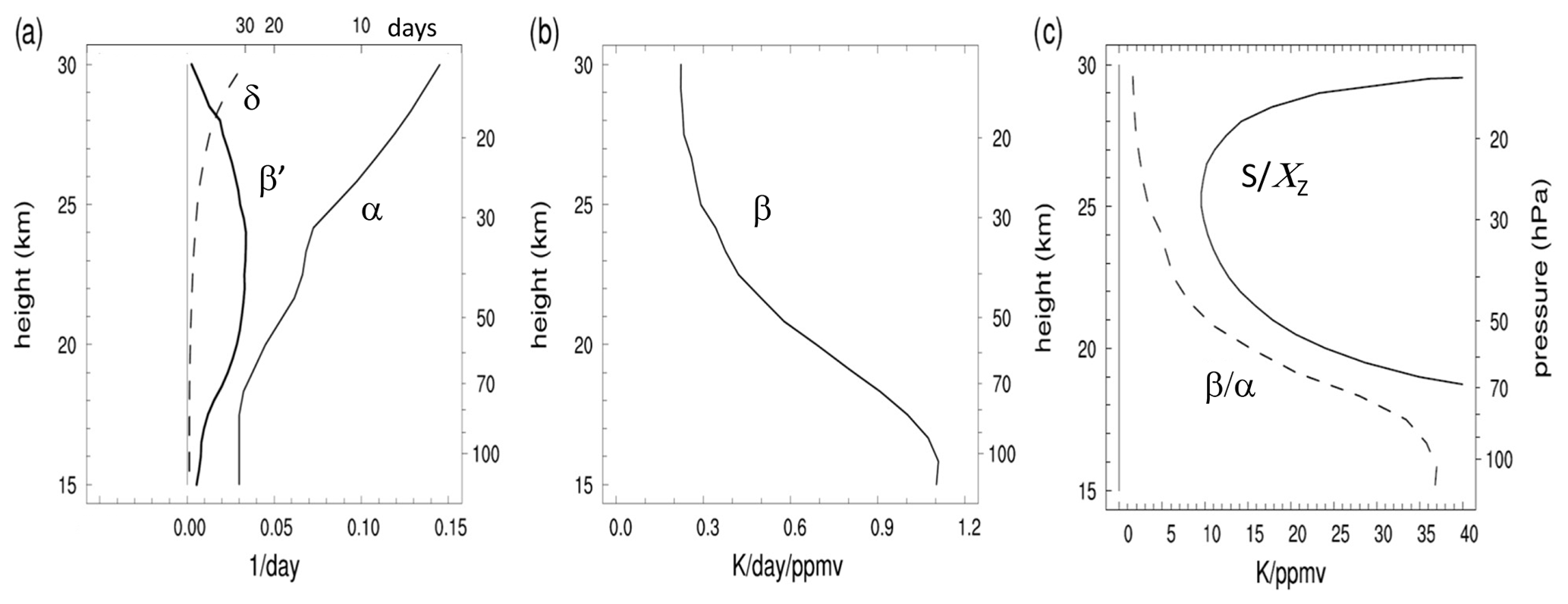
Figure 1Vertical profiles of parameters used in the theoretical model calculations: (a) α, β′, and δ; (b) β; and (c) ( and (. The top axis in (a) shows the associated timescales in days.
We estimate vertical profiles of the parameter β from radiative transfer calculations using a modified version of the Morcrette (1991) radiation scheme (Zhong and Haigh, 1995). The calculations use realistic background temperature, ozone and water vapor profiles, and carbon dioxide is assumed to be well mixed with a volume mixing ratio of 360 ppmv. Shortwave heating rates are calculated as diurnal averages, including realistic surface albedo, and all calculations assume clear-sky conditions. β is derived by applying a 0.1 ppmv perturbation to the ozone field at each vertical level and calculating the ratio of the instantaneous heating rate change at that level to the amplitude of the ozone perturbation. The resulting profile of β is shown in Fig. 1b, with typical values of 0.3–1.0 (K/d/ppmv), decreasing in altitude away from the tropopause. The vertical structure of ) β is included in Fig. 1a, showing a magnitude somewhat smaller than α throughout the profile. This in turn implies a positive ( from Eqs. (8) to (9b) (including a realistic small δ); i.e., temperature leads ozone in the coupled response based on these parameters, although as shown below the phase difference turns out to be small. Vertical profile of the quantity ( (zero frequency limit for (, for small δ) is included in Fig. 1c, showing a decrease from the tropopause to the middle stratosphere with values substantially smaller than (.
We derived an estimate of the damping rate δ(z) for ozone from simulations of the Whole Atmosphere Community Climate Model (WACCM; Marsh et al., 2013), which includes a sophisticated stratospheric ozone chemical scheme. These calculations use daily zonal average output of ozone amount (X) and photochemical ozone loss rate (L) as a function of latitude and altitude, and we take an annual average of their ratio: , averaging results over 10∘ N–S. The resulting vertical profile of δ is shown in Fig. 1a, showing very small damping (long ozone lifetimes) in the lower stratosphere, increasing to slightly larger values in the middle stratosphere (damping timescale of ∼ 30 d at 30 km). Calculations below show idealized model results including these realistic values of δ, and for comparison we also include results for δ=0. Including realistic values of ozone damping has almost no influence on calculations in the lower stratosphere because of the very small damping. Damping can have a small but noticeable effect at higher altitudes for lower-frequency variations (increasing the ratios) but still only accounts for a ∼ 10 % effect.
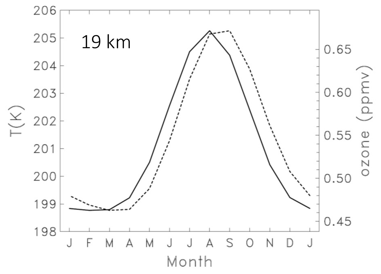
Figure 2Climatological annual cycles of ozone (dashed line) and temperature (solid line) at 19 km derived from SHADOZ measurements over 1998–2016.
4.1 Annual and QBO variability in SHADOZ ozone and temperature
The approximately monthly sampling of SHADOZ data allows for characterization of the annual cycle and interannual variations of tropical stratospheric ozone and temperature. There is a relatively large annual cycle in ozone and temperature in the tropical lower stratosphere over ∼ 16–22 km, with relative maxima during boreal summer and temperature slightly leading ozone in time. Figure 2 shows this behavior for the 19 km level, near the peak of the annual cycle. This correlated ozone–temperature behavior is mainly a response to the annual cycle in tropical upwelling (Randel et al., 2007); horizontal transport from the boreal summer monsoons also contributes to the seasonal maximum in ozone close to the tropopause (Konopka et al., 2009, 2010; Stolarski et al., 2014; Tweedy et al., 2017), but mean upwelling is the dominant mechanism above 18 km (Abalos et al., 2013). Above 23 km, the annual cycle becomes small and the dominant seasonal variation becomes semiannual in both ozone and temperature. We note that the seasonal variations in Fig. 2 are very similar based on the MLS ozone and GPS temperature data (not shown).
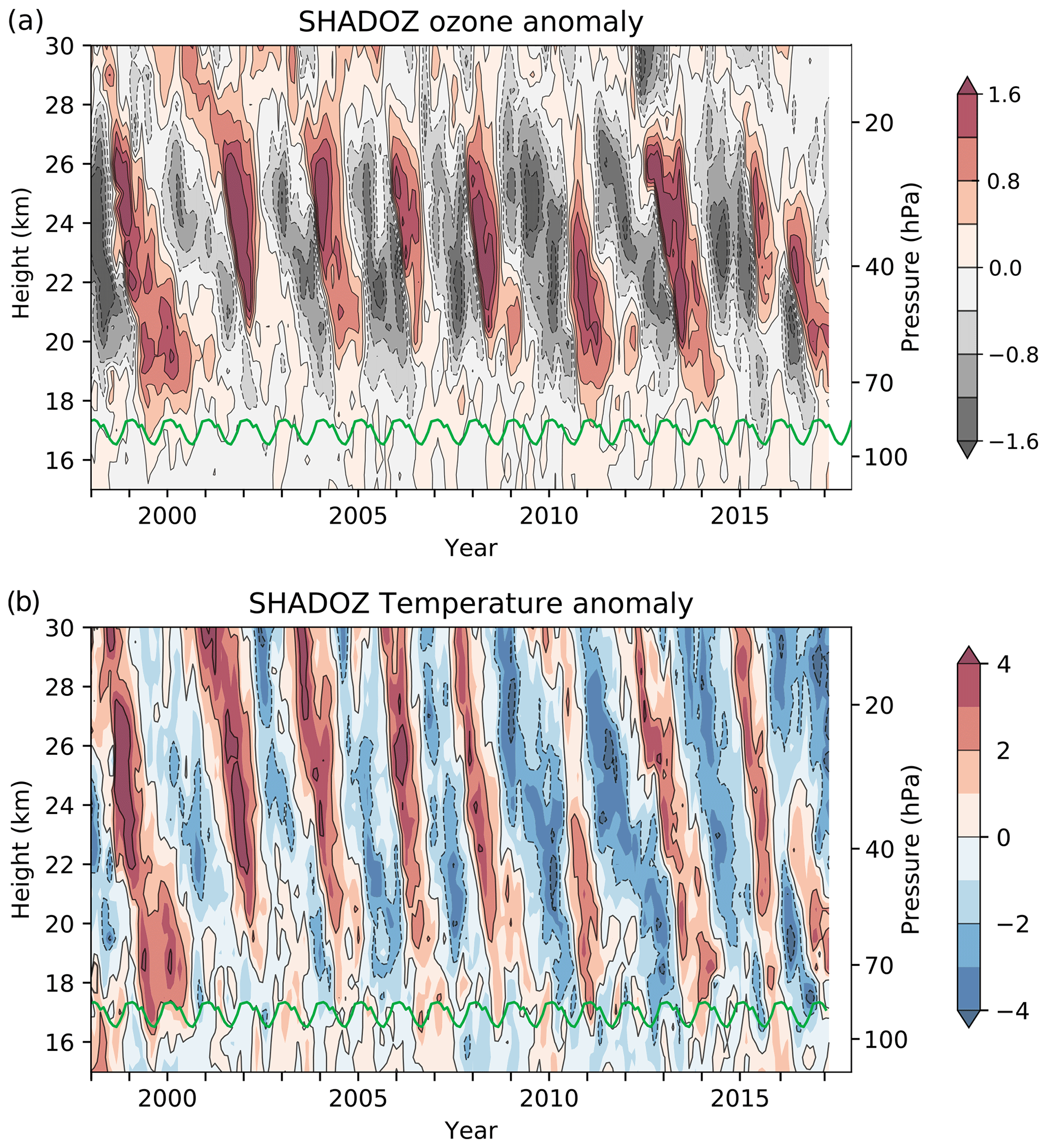
Figure 3Height–time sections of deseasonalized anomalies in (a) ozone and (b) temperature (K) from SHADOZ data. Ozone anomalies are expressed in terms of ozone density (DU/km) to emphasize variability throughout the lower stratosphere. The green lines denote the cold-point tropopause.
Interannual anomalies in ozone and temperature from SHADOZ data over 1998–2016 are shown in Fig. 3, derived by simply subtracting the mean annual cycle. In Fig. 3 ozone anomalies are shown in terms of ozone density (DU/km) instead of mixing ratio, in order to emphasize variations throughout the lower stratosphere. As is well known, there are strong downward propagating anomalies in ozone and temperature linked to the QBO; the ozone and temperature anomalies are approximately in phase over ∼ 17–27 km, and the variations in ozone are small above 27 km due to a transition from dynamical control in the lower stratosphere to photochemical control above ∼ 27 km (e.g., Chipperfield and Gray, 1992; Park et al., 2017). Episodic ENSO events also result in correlated ozone–temperature variations in the tropical lower stratosphere for levels from the tropopause to ∼ 22 km (Randel et al., 2009; Calvo et al., 2010). The constructive interference of QBO and ENSO effects can result in large anomalies near and above the tropopause (e.g., Diallo et al., 2018), as seen for the SHADOZ data in 1999–2000 and 2015–2016.
Figure 4 shows the ozone–temperature correlation derived from the deseasonalized SHADOZ data (from Fig. 3) as a function of altitude and time lag. Strong positive correlations (> 0.8) are found over 17–27 km, as expected from Fig. 3. The strongest correlations occur near zero time lag, but the lag correlations are skewed towards positive lags, which is a signature of temperature leading ozone anomalies by a small amount, similar to the annual cycle in Fig. 2.
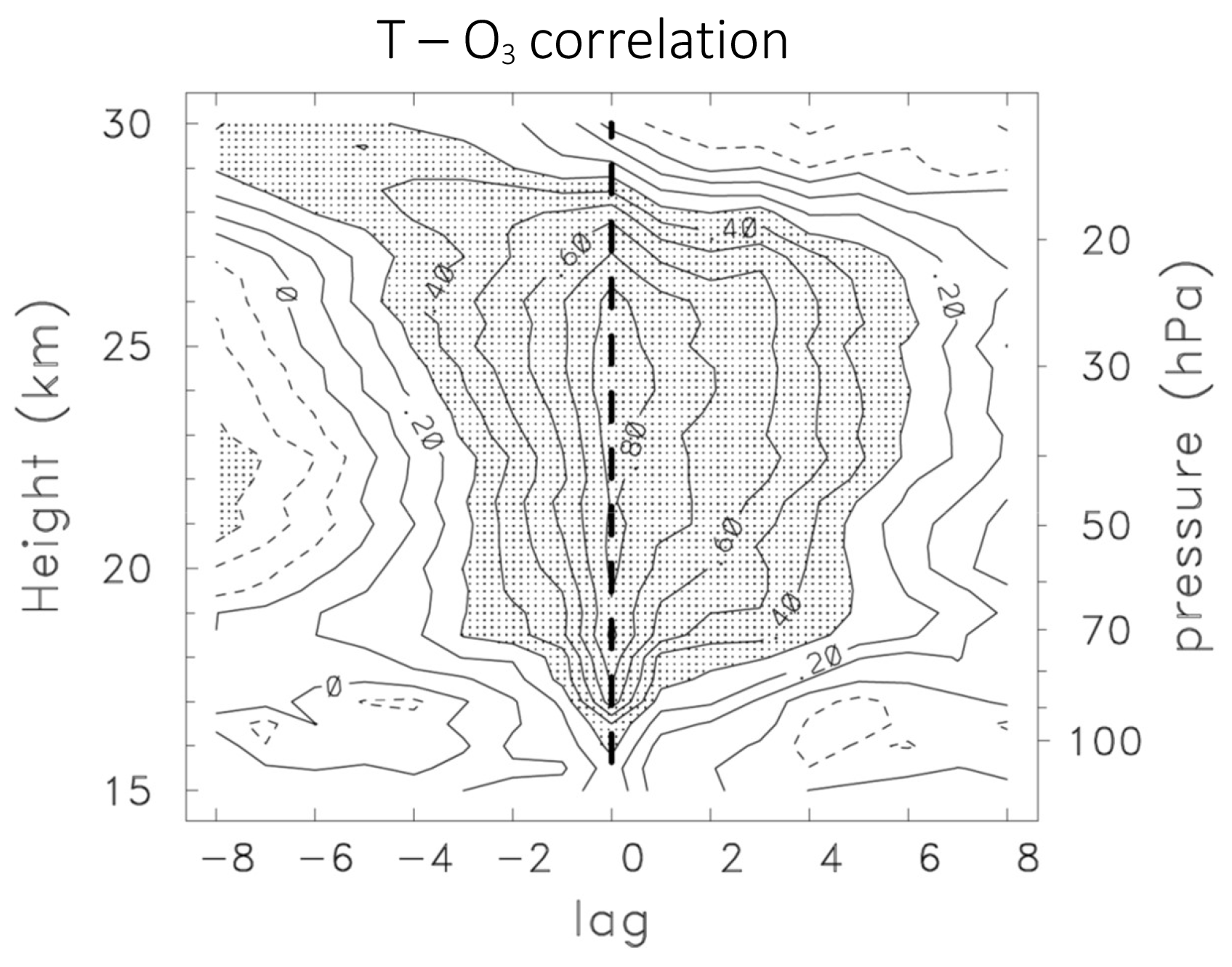
Figure 4Correlation of deseasonalized SHADOZ ozone and temperature time series as a function of height and time lag (in months). Positive lag denotes temperature leading ozone.
A scatterplot of the SHADOZ temperature vs. ozone deseasonalized anomalies at 24 km over 1998–2016 is shown in Fig. 5, highlighting the strong observed correlation. The slope of the (T O3) variations is near 6.1 (K/ppmv). This slope changes as a function of altitude (as shown below), and this is one of the quantities that we aim to understand from a simple perspective.
4.2 Satellite observations
We use MLS and GPS satellite data to quantify ozone–temperature correlations over a continuous range of time scales from days to over a decade. Time series of zonal mean GPS temperatures and MLS ozone over the Equator (10∘ N–S) at 24 km (31 hPa for MLS) are shown in Fig. 6 for pentad averages covering September 2004–March 2018. Visual inspection of Fig. 6 shows the clear signature of the QBO (as in Fig. 3) and strong correlations of ozone and temperature across all scales of variability, including both long- and short-term fluctuations.
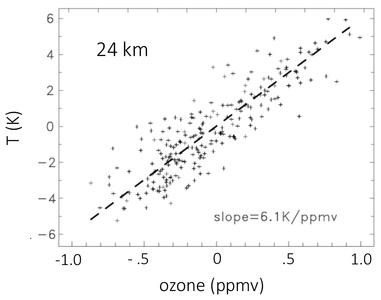
Figure 5Scatterplot of deseasonalized temperature vs. ozone anomalies from SHADOZ data at 24 km (data as in Fig. 3).
Power spectra for temperature and ozone at 24 km are shown in Fig. 7a. In these and the following spectral plots, the ordinate shows the wave period (from 10 to 4990 d) using a logarithmic frequency axis in order to more clearly separate low- and high-frequency behavior. The spectra for both quantities show the most power at low frequencies, with peaks linked to the QBO, annual and semiannual cycles. At altitudes below 24 km the annual cycle is more pronounced, while above 24 km the semiannual cycle is larger. Power decreases systematically at periods shorter than semiannual for both ozone and temperature in Fig. 7a. Temperature-ozone coherence squared (coh2) at 24 km is shown in Fig. 7b, highlighting significant values over nearly the entire range of periods longer than ∼ 20 d. There is a relative minimum in coh2 near the semiannual cycle, and this could possibly be related to the semiannual variation in low-latitude ozone photochemical production noted above, which adds additional ozone variability that is less coherent with temperature. The reason for the lack of coherence at the shortest resolved timescales (< 20 d) is unknown but could be related to the very low power in both data sets (Fig. 7a) and poorer temporal resolution of these time scales based on pentad data. There is a relatively small phase difference between ozone and temperature over all frequencies, as shown below. Similar behavior is found for temperature-ozone coh2 and phase for all altitudes over 17–27 km. Above 29 km there is a strong coh2 maximum for the semiannual oscillation (∼ 180 d period), where ozone and temperature are approximately out of phase (not shown). This behavior is due to the transition to photochemical control of ozone and the impact of temperature on the odd-oxygen (Ox) loss rate (Brasseur and Solomon, 2005).
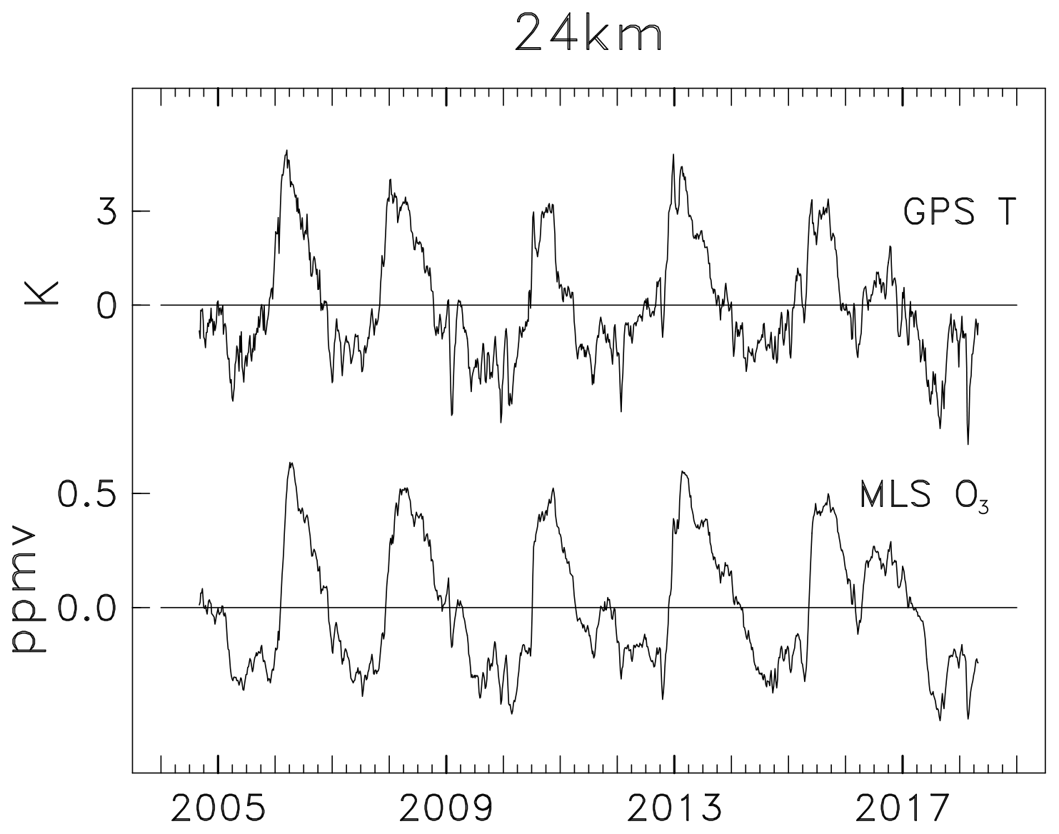
Figure 6Time series of zonal average GPS temperatures and MLS ozone at 24 km for averages over 10∘ N–S.
We next compare frequency-dependent ( amplitude and phase between observations and results from the idealized model calculations (Eq. 9a–b). Figure 8a compares observed and modeled 24 km ( amplitude as a function of frequency. Observations are based on the GPS temperature and MLS ozone results, where ( is calculated from the respective harmonic coefficients and the ratio is smoothed in frequency. Model results are shown with and without including ozone damping effects, which has relatively small influence, along with calculations neglecting ozone feedback effects on temperature (β=0). Additionally, Fig. 8a includes the ( ratio estimated from deseasonalized SHADOZ anomalies (from Fig. 5) which are mainly associated with the QBO (∼ 28-month period). The observed ( ratio shows a systematic change over the frequency range, with approximately a factor of 2 decrease in the ratio for low frequencies (periods > 150 d) compared to high frequencies. The idealized model results show a similar ( frequency dependence, albeit with substantial disagreement on the detailed shape of the transition region between semiannual and interannual (QBO) periods, with a slower transition in the model. This disagreement is not understood but might be related to the semiannual ozone photochemical production term over the Equator discussed above, which is not included in the model calculations. The overall systematic change with frequency in Fig. 8a corresponds to the change from ozone–temperature coupling via transport (high frequency) to radiative balance (low frequency). Including the ozone damping (δ) slightly improves the agreement at low frequencies.
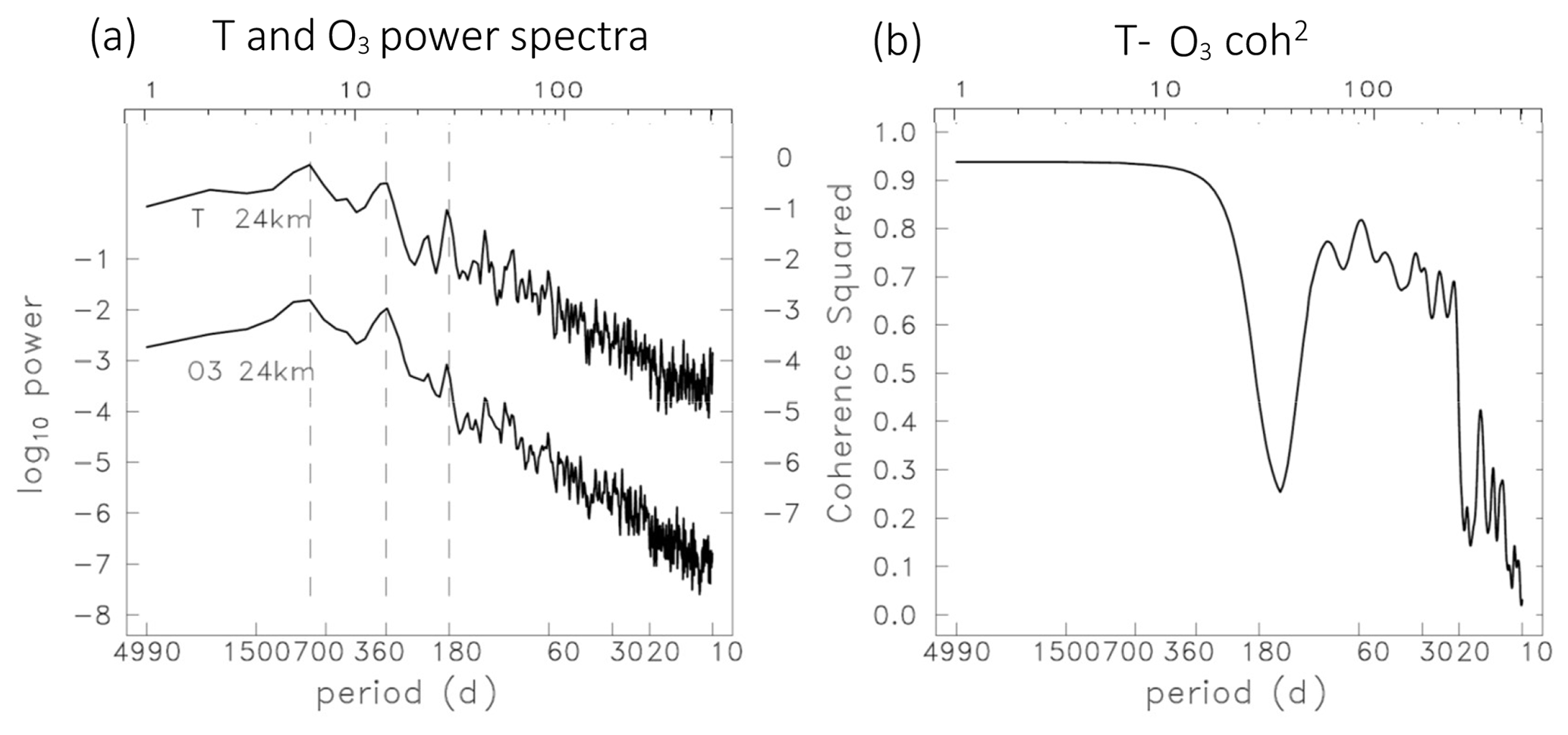
Figure 7(a) Power spectra for GPS temperature and MLS ozone at 24 km as a function of wave period. Logarithmic power units are K2 (right axis) and ppmv2 (left axis). The vertical dashed lines identify peaks in the spectra associated with the QBO, annual and semiannual cycles. The top logarithmic axis indicates the spectral estimates. (b) Coherence squared between temperature and ozone at 24 km as a function of wave period.
Differences between the full model and β=0 results in Fig. 8a quantify the ozone feedback on temperature in the coupled system. Ozone radiative feedback is mainly important for low-frequency (“slow”) variability and becomes increasingly important for the longest timescales. For example, for the QBO time period (28 months) the ozone feedback increases the ( ratio at 24 km by approximately 40 %, with even larger effects at lower frequencies. We note that this increasing importance of ozone feedbacks for low frequencies is consistent with the results of Charlesworth et al. (2019).
The observed and modeled ( phase relationship as a function of frequency is shown in Fig. 8b, showing approximately in-phase behavior across all frequencies in both cases. The model ( phase is slightly positive (as expected from Sect. 3) and in approximate agreement with observed results. Similar behavior to Fig. 8 is found in the satellite data for all altitudes over 19–27 km. Neglecting ozone feedbacks (β=0) gives worse agreement with observations.
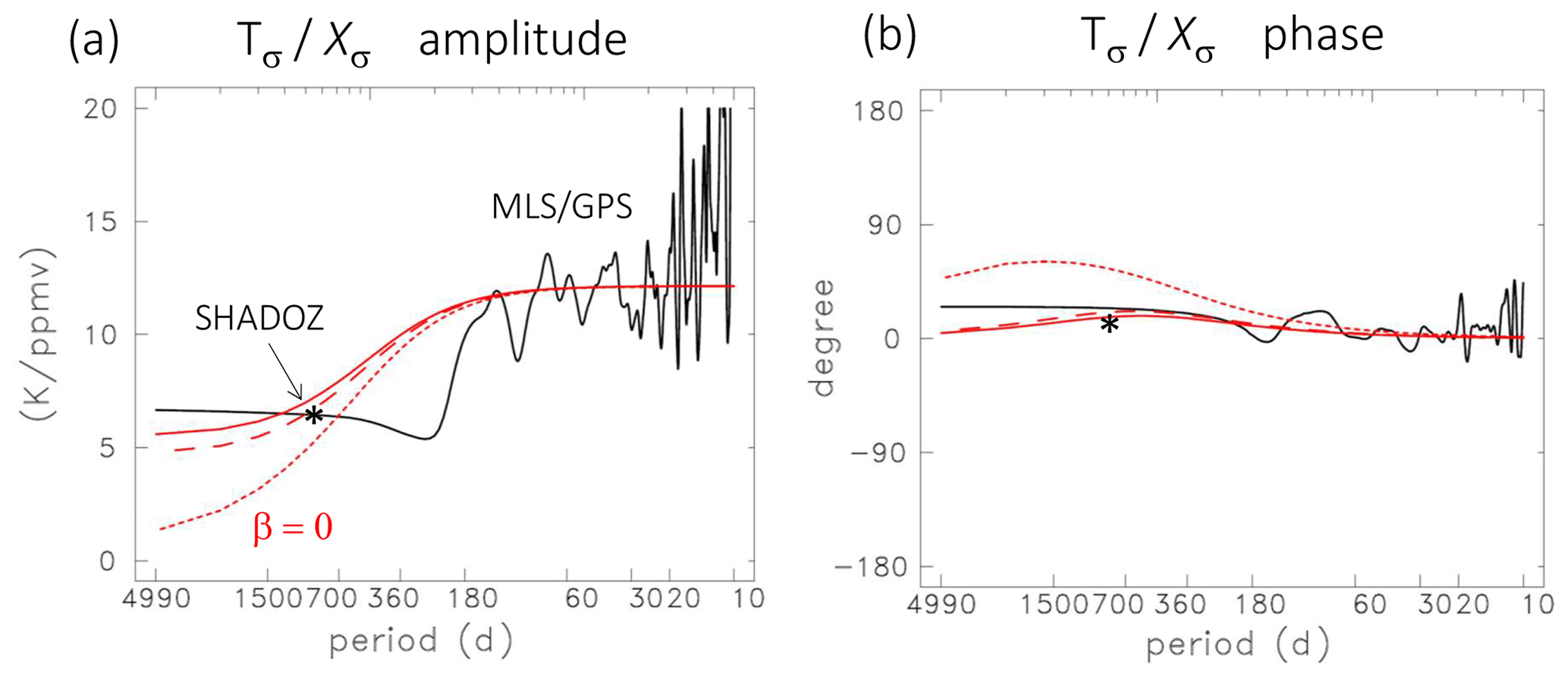
Figure 8(a) ( ratio at 24 km as a function of wave period. The black line shows observational results from MLS and GPS satellite data, and the red lines show idealized model calculations (the solid red line includes ozone damping, the dashed red line is for δ=0 and the dotted red line is for β=0). The ( ratio derived from deseasonalized SHADOZ data at 24 km (Fig. 5) is also shown, which is mainly associated with the QBO (∼ 28-month period). (b) Corresponding ( phase differences.
Vertical profiles of observed and modeled ( amplitude are shown in Fig. 9 for three different frequency bands, corresponding to “fast” frequencies (30–60 d period, Fig. 9a), the annual cycle (Fig. 9b) and the QBO (Fig. 9c). In addition to observations from the MLS and GPS data, we include the corresponding ratios calculated from SHADOZ ozone and temperature data for the annual cycle (e.g., Fig. 2a), calculated as the ratio of the respective ozone and temperature maximum-minimum values over the annual cycle, for altitudes 19–23 km where the annual cycle is distinct in the data. Figure 9c includes SHADOZ results for deseasonalized anomalies, which are mainly linked to the QBO and derived from regression as in Fig. 5. These SHADOZ results in Fig. 9b–c agree well with the corresponding estimates from MLS and GPS satellite data. The fast frequencies (Fig. 9a) are governed by vertical transport with a ( vertical profile close to ( (Fig. 1c), and the model shows a good fit to the observed vertical structure, at least up to ∼ 27 km. The annual cycle (Fig. 9b) is close to the cross-over between high- and low-frequency behavior, and the model again shows approximate agreement to observations over altitudes where the annual cycle is large (∼ 19–23 km). This agreement helps confirm the interpretation that the annual cycles in tropical stratospheric temperature and ozone (e.g., Fig. 2) can be interpreted as coupled responses to the annual cycle in tropical upwelling, with ozone feeding back on temperature. For the lower-frequency QBO variations (Fig. 9c) the idealized model shows good agreement with the ( amplitude from both the satellite data and SHADOZ throughout the profile. Our conclusions from these comparisons is that the idealized model can quantitatively explain the observed ( amplitude and phase relationships in the tropical lower stratosphere, including their dependence on frequency and altitude.

Figure 9Vertical profiles of ( amplitude for selected frequency bands: (a) 30–60 d periods, (b) the annual cycle (12-month period) and (c) the QBO period (∼ 28 months). The solid black lines are results from MLS and GPS satellite data, and the red lines show idealized model calculations (the solid red line includes ozone damping, dashed red lines are for δ=0 and dotted red lines are for β=0). Additionally, results from SHADOZ ozone and temperature data are included as dashed black lines in (b–c), as described in text. Observations for the annual cycle (b) are only shown over altitudes 19–23 km where the annual cycle is relatively large and distinct.
Observations show strong correlations between ozone and temperature in the tropical lower stratosphere, and calculations show that the ozone radiative feedbacks significantly enhance temperatures, e.g., by ∼ 30 % for the annual cycle (e.g., Ming et al., 2017). This ozone feedback significantly enhances thermal variability in global model simulations (Yook et al., 2020). The goals of this work include providing an update of observational evidence for T–O3 coupling and simplified understanding based on idealized zonal mean theory. The excellent long-term tropical ozonesonde measurements from SHADOZ demonstrate approximate in-phase T–O3 correlations for the annual cycle (Fig. 2) and for interannual anomalies (Figs. 3–5), which are dominated by the QBO. Long-term continuous satellite measurements from zonal average MLS and GPS data agree well with these results for annual and interannual variations, and furthermore demonstrate strong T–O3 coherence for faster sub-seasonal variability (Figs. 6–7b). This coherent behavior is observed throughout the lower to middle stratosphere, ∼ 17–27 km, with T–O3 anomalies approximately in phase over all altitudes. A key result is that the observed (T O3) ratio changes as a function of frequency, with approximately half the ratio for low frequencies (annual cycle and longer) compared to faster variability (Fig. 8a). The (T O3) ratio also depends on altitude, with much larger ratios for levels in the lower stratosphere (Fig. 9). These are the key observational characteristics of T–O3 coupling that we seek to explain.
We compare observations to results from idealized zonal mean theory, assuming vertical advection from the upward Brewer–Dobson circulation controls thermal balances and ozone transport, i.e., neglecting mean meridional advection and eddy transport terms. This is a reasonable approximation in the tropical lower stratosphere above the tropical tropopause layer (TTL) (Abalos et al., 2013), although eddy transport from monsoon circulations makes important contributions to ozone tendencies during boreal summer at and below ∼ 18 km (Konopka et al., 2009, 2010; Stolarski et al., 2014). Thermodynamic balance includes linear radiative damping (α) and ozone feedback (β) terms, and the coupled equations (including linear ozone damping δ) can be solved analytically to calculate the (T O3) ratio as a function of frequency and altitude, dependent on model parameters α, β and δ and the ratio of background gradients expressed as (. In general, ozone damping is a minor influence over most of the domain because of the long ozone lifetimes. The model balances highlight two timescales for T–O3 coupling, including fast variability, where the (T O3) ratio is determined by the background vertical gradients (, and slow timescales determined by radiative balance ( in the zero-frequency limit). The idealized model shows a functional frequency dependence for the (T O3) ratio similar to observations (Fig. 8a), although there is disagreement in the transition region where the observations show a more rapid (T O3) transition with a slight minimum near the semiannual period. This detail is not well understood but could be influenced by a semiannual ozone photochemical production term in the equatorial region related to solar inclination (Abalos et al., 2013) that is not included in our model, along with neglected eddy transport effects, especially near the tropopause. This semiannual ozone production may also explain the relative minimum in T–O3 coherence squared near this frequency found in Fig. 7b. The vertical profiles of (T O3) ratio agree well with the observations for both fast (Fig. 9a) and slow (Fig. 9b–c) timescales, enhancing confidence in a simple understanding.
Ozone feedback on temperature is easy to quantify in our model by comparing results neglecting the feedback (β=0). Results show important ozone feedbacks for low-frequency variations (i.e., the slow regime), and the feedback becomes increasingly important at lower frequencies (e.g., Fig. 8a). We note that the frequency-dependent T–O3 ozone feedback shown here is consistent with the results of Charlesworth et al. (2019), which show larger ozone radiative impacts on tropopause temperatures for low frequencies.
One further aspect of coupled T–O3 behavior can be deduced from Eq. (3), noting that the α and β terms are closely coupled by observed T–O3 correlations in the lower stratosphere. Using the empirical approximation , where and likewise for ΔT, the combined terms ( in Eq. (3) can be rewritten as (. These terms can be combined into −αeffΔT, with representing an “effective” thermal damping timescale combining both radiative relaxation and ozone feedback effects. Using realistic α and β′ values (Fig. 1a), αeff is significantly smaller than α alone; i.e., the ozone feedback increases the radiative damping timescale compared to radiative relaxation alone. This result is consistent with the effective timescales inferred by Fueglistaler et al. (2014) and with the coupled chemistry–climate model calculations in Yook et al. (2020), their Fig. 6. Alternatively, since the ozone radiative feedback arises primarily from transport effects, its effect can also be viewed as an enhancement to the dynamical heating.
It is worthwhile to appreciate the limitations associated with the idealized model calculations, especially uncertainties related to the parameters α and β, which control the low-frequency model behavior. While Hitchcock et al. (2010) show that linear regression on temperature captures ∼ 80 % of the variance in modeled radiative heating rates in the tropical lower stratosphere, the broad spectrum of vertical scales in this region can introduce additional uncertainties in estimating α. Our calculations of ozone heating via the β term in Eq. (3) neglects the effects of non-local ozone changes, which will also depend in detail on the vertical scale of perturbations. In spite of these caveats, the overall agreement between model and observations demonstrates that the idealized zonal mean theory (quantifying coupled T–O3 response to variations in the Brewer–Dobson circulation) is a valid perspective to understand the strong T–O3 coupling in the real atmosphere.
SHADOZ data were obtained from the SHADOZ website https://tropo.gsfc.nasa.gov/shadoz/ (last access: 10 December 2021). MLS ozone data were obtained from https://mls.jpl.nasa.gov/index-eos-mls.php (last access: 10 December 2021). GPS temperatures were obtained from the COSMIC Data Analysis and Archive Center (CDACC) website https://cdaac-www.cosmic.ucar.edu/ (last access: 10 December 2021).
The study was conceived by WJR, and data analysis was performed by FW. AM and PH provided input for the idealized model calculations and contributed to interpretation of results. The paper was written by WJR, with editing from AM and PH.
The contact author has declared that neither they nor their co-authors have any competing interests.
Publisher’s note: Copernicus Publications remains neutral with regard to jurisdictional claims in published maps and institutional affiliations.
The National Center for Atmospheric Research is sponsored by the U.S. National Science Foundation. This work has been partially supported by the COSMIC NSF-NASA Cooperative Agreement under grant no. 1522830, and by the NASA Aura Science Team under grant no. 80NSSC20K0928. AM would like to acknowledge support from the Leverhulme Trust as an early career fellow. We thank Marta Abalos, Rolando Garcia, Paul Konopka, and Lan Luan for discussions and comments that significantly improved the manuscript and two anonymous reviewers for constructive reviews.
This research has been supported by the NASA Earth Sciences Division (grant no. 80NSSC20K0928).
This paper was edited by Rolf Müller and reviewed by two anonymous referees.
Abalos, M., Randel, W. J., and Serrano, E.: Variability in upwelling across the tropical tropopause and correlations with tracers in the lower stratosphere, Atmos. Chem. Phys., 12, 11505–11517, https://doi.org/10.5194/acp-12-11505-2012, 2012.
Abalos, M., Randel, W. J., Kinnison, D. E., and Serrano, E.: Quantifying tracer transport in the tropical lower stratosphere using WACCM, Atmos. Chem. Phys., 13, 10591–10607, https://doi.org/10.5194/acp-13-10591-2013, 2013.
Andrews, D. G., Holton, J. R., and Leovy, C. B.: Middle Atmosphere Dynamics, Academic Press, 489 pp., 1987.
Anthes, R. A., Bernhardt, P. A., Chen, Y., Cucurull, L., Dymond, K. F., Ector, D., Healy, S. B., Ho, S.-P., Hunt, D.C., Kuo, Y.-H., Liu, H., Manning, K., McCormick, C., Meehan, T. K., Randel, W. J., Rocken, C., Schreiner, W. S., Sokolovskiy, S. V., Syndergaard, S., Thompson, D. C., Trenberth, K. E., Wee, T.-K., Yen, N. L., and Zeng, Z.: The COSMIC/FORMOSAT-3 Mission: Early results, B. Am. Meteorol. Soc., 89, 313–333, 2008.
Baldwin, M. P., Gray, L. J., Dunkerton, T. J., Hamilton, K., Haynes, P. H., Randel, W. J., Holton, J. R., Alexander, M. J., Hirota, I., Horinouchi, T., Jones, D. B. A., Kinnersley, J. S., Marquardt, C., Sato, K. and Takahashi, M.: The Quasi-Biennial Oscillation, Rev. Geophys., 39, 179–229, 2001.
Birner, T. and Charlesworth, E. J.: On the relative importance of radiative and dynamical heating for tropical tropopause temperatures, J. Geophys. Res.-Atmos., 122, 6782–6797, https://doi.org/10.1002/2016JD026445, 2017.
Brasseur, G. and Solomon, S.: Aeronomy of the Middle Atmosphere, Springer, https://doi.org/10.1007/1-4020-3824-0, 644 pp., 2005.
Calvo, N., García, R. R., Randel, W. J., and Marsh, D. R.: Dynamical mechanism for the increase in tropical upwelling in the lowermost tropical stratosphere during warm ENSO events, J. Atmos. Sci., 67, 2331–2340, https://doi.org/10.1175/2010JAS3433.1, 2010.
Chae, J. H. and Sherwood, S. C.: Annual temperature cycle of the tropical tropopause: A simple model study, J. Geophys. Res., 112, D19111, https://doi.org/10.1029/2006JD007956, 2007.
Charlesworth, E. J., Birner, T., and Albers, J. R.: Ozone transport-radiation feedbacks in the tropical tropopause layer, Geophys. Res. Lett., 46, https://doi.org/10.1029/2019GL084679, 2019.
Chipperfield, M. P. and Gray, L. J.: Two-dimensional model studies of the interannual variability of trace gases in the middle atmosphere, J. Geophys. Res., 97, 5963–5980, https://doi.org/10.1029/92JD00029, 1992.
Dacie, S., Kluft, L., Schmidt, H., Stevens, B., Buehler, S. A., Nowack, P. J., Dietmuller, S., Abraham, N. L., and Birner, T.: A 1D RCE study of factor affecting the tropical tropopause layer and surface climate, J. Climate, 32, 6769–6782, https://doi.org/10.1175/JCLI-D-18-0778.1, 2019.
Diallo, M., Riese, M., Birner, T., Konopka, P., Müller, R., Hegglin, M. I., Santee, M. L., Baldwin, M., Legras, B., and Ploeger, F.: Response of stratospheric water vapor and ozone to the unusual timing of El Niño and the QBO disruption in 2015–2016, Atmos. Chem. Phys., 18, 13055–13073, https://doi.org/10.5194/acp-18-13055-2018, 2018.
Forster, P. M., Bodeker, G., Schofield, R., Solomon, S., and Thompson, D.: Effects of ozone cooling in the tropical lower stratosphere and upper troposphere, Geophys. Res. Lett., 34, L23813, https://doi.org/10.1029/2007GL031994, 2007.
Fueglistaler, S., Haynes, P. H., and Forster, P. M.: The annual cycle in lower stratospheric temperatures revisited, Atmos. Chem. Phys., 11, 3701–3711, https://doi.org/10.5194/acp-11-3701-2011, 2011.
Fueglistaler, S., Abalos, M., Flannaghan, T. J., Lin, P., and Randel, W. J.: Variability and trends in dynamical forcing of tropical lower stratospheric temperatures, Atmos. Chem. Phys., 14, 13439–13453, https://doi.org/10.5194/acp-14-13439-2014, 2014.
Gilford, D. M., Solomon, S., and Portmann, R. W.: Radiative impacts of the 2011 abrupt drops in water vapor and ozone in the tropical tropopause layer, J. Climate, 29, 595–612, https://doi.org/10.1175/JCLI-D-15-0167.1, 2016.
Gilford, D. and Solomon, S.: Radiative effects of stratospheric seasonal cycles in the tropical upper troposphere and lower stratosphere, J. Climate, 30, 2769–2783, https://doi.org/10.1175/JCLI-D-16-0633.1, 2017.
Hartmann, D. L., Holton, J. R., and Fu, Q.: The heat balance of the tropical tropopause, cirrus and stratospheric dehydration, Geophys. Res. Lett., 28, 1969–1972, 2001.
Hasebe, F.: Quasi-biennial oscillations of ozone and diabatic circulation in the equatorial stratosphere, J. Atmos. Sci., 51, 729–745, https://doi.org/10.1175/1520-0469(1994)051<0729:QBOOOA>2.0.CO;2, 1994.
Hauchecorne, A., Bertaux, J. L., Dalaudier, F., Keckhut, P., Lemennais, P., Bekki, S., Marchand, M., Lebrun, J. C., Kyrölä, E., Tamminen, J., Sofieva, V., Fussen, D., Vanhellemont, F., Fanton d'Andon, O., Barrot, G., Blanot, L., Fehr, T., and Saavedra de Miguel, L.: Response of tropical stratospheric O3, NO2 and NO3 to the equatorial Quasi-Biennial Oscillation and to temperature as seen from GOMOS/ENVISAT, Atmos. Chem. Phys., 10, 8873–8879, https://doi.org/10.5194/acp-10-8873-2010, 2010.
Hitchcock, P., Shepherd, T. G., and Yoden, S.: On the approximation of local and linear radiative damping in the middle atmosphere, J. Atmos. Sci., 67, 2070–2085, https://doi.org/10.1175/2009JAS3286.1, 2010.
Jenkins, G. M. and Watts, D. G.: Spectral Analysis and Its Applications, Holden-Day, 525 pp., 1968.
Konopka, P., Grooß, J., Ploeger, F., and Müller, R.: Annual cycle of horizontal in-mixing into the lower tropical stratosphere, J. Geophys. Res., 114, D19111, https://doi.org/10.1029/2009JD011955, 2009.
Konopka, P., Grooß, J.-U., Günther, G., Ploeger, F., Pommrich, R., Müller, R., and Livesey, N.: Annual cycle of ozone at and above the tropical tropopause: observations versus simulations with the Chemical Lagrangian Model of the Stratosphere (CLaMS), Atmos. Chem. Phys., 10, 121–132, https://doi.org/10.5194/acp-10-121-2010, 2010.
Livesey, N. J., Read, W. G., Wagner, P. A., Froidevaux, L., Lambert, A., Manney, G. L., Millán Valle, L. F., Pumphrey, H. C., Santee, M. L., Schwartz, M. L., Wang, S., Fuller, R. A., Jarnot, R. F., Knosp, B. W., Martinez, E., and Lay, R. L.: Aura Microwave Limb Sounder (MLS) version 4.2x level 2 data quality and description document, Tech. Rep., Jet Propulsion Laboratory, available at: https://mls.jpl.nasa.gov/data/v4-2_data_quality_document.pdf (last access: 10 December 2021), 2018.
Marsh, D., Mills, M., Kinnison, D. E., and Lamarque, J. -F.: Climate change from 1850 to 2005 simulated in CESM1(WACCM), J. Climate, 26, 7372–7391, https://doi.org/10.1175/JCLI-D-12-00558.1, 2013.
Ming, A., Maycock, A. C., Hitchcock, P., and Haynes, P.: The radiative role of ozone and water vapour in the annual temperature cycle in the tropical tropopause layer, Atmos. Chem. Phys., 17, 5677–5701, https://doi.org/10.5194/acp-17-5677-2017, 2017.
Morcrette, J.-J.: Radiation and cloud radiative properties in the European Centre for Medium Range Weather Forecasts forecasting system, J. Geophys. Res.-Atmos., 96, 9121–9132, https://doi.org/10.1029/89JD01597, 1991.
Newman, P. A. and Rosenfield, J. E.: Stratospheric thermal damping times, Geophys. Res. Lett., 24, 433–436, 1997.
Park, M., Randel, W. J., Kinnison, D. E., Bourassa, A. E., Degenstein, D. A., Roth, C. Z., McLinden, C. A., Sioris, C. E., Livesey, N. E., and Santee, M. L.: Variability of stratospheric reactive nitrogen and ozone related to the QBO, J. Geophys. Res., 122, https://doi.org/10.1002/2017JD027061, 2017.
Polvani, L. M. and Solomon, S.: The signature of ozone depletion on tropical temperature trends, as revealed by their seasonal cycle in model integrations with single forcings, J. Geophys. Res., 117, D17102, https://doi.org/10.1029/2012JD017719, 2012.
Randel, W. J., Park, M., Wu, F., and Livesey, N.: A large annual cycle in ozone above the tropical tropopause linked to the Brewer-Dobson circulation, J. Atmos. Sci., 64, 4479–4488, 2007.
Randel, W. J., Garcia, R. R., Calvo, N., and Marsh, D.: ENSO influence on zonal mean temperature and ozone in the tropical lower stratosphere, Geophys. Res. Lett., 36, L15822, https://doi.org/10.1029/2009GL039343, 2009.
Randel, W. J. and Thompson, A. M.: Interannual variability and trends in tropical ozone derived from SAGE II satellite data and SHADOZ ozonesondes, J. Geophys. Res., 116, D07303, https://doi.org/10.1029/2010JD015195, 2011.
Randel, W. J. and Wu, F.: Variability of zonal mean tropical temperatures derived from a decade of GPS radio occultation data, J. Atmos. Sci., 72, 1261–1275, https://doi.org/10.1175/JAS-D-14-0216.1, 2015.
Stolarski, R. S., Waugh, D. W., Wang, L., Oman, L. D., Douglass, A. R., and Newman, P. A.: Seasonal variation of ozone in the tropical lower stratosphere: Southern tropics are different from northern tropics, J. Geophys. Res.-Atmos., 119, 6196–6206, https://doi.org/10.1002/2013JD021294, 2014.
Thompson, A. M. Witte, C., McPeters, R. D., Oltmans, S. J., Schmidlin, F. J., Logan, J. A., Fujiwara, M., Kirchoff, V. W., Posny, F., Coetzee, G. J. R., Hoegger, B., Kawakami, S., Ogawa, T., Johnson, B. J., Vomel, H., and Labow, G.: Southern Hemisphere Additional Ozonesondes (SHADOZ) 1998–2000 tropical ozone climatology: 1. Comparison with Total Ozone Mapping Spectrometer (TOMS) and ground-based measurements, J. Geophys. Res.-Atmos., 108, 8238, https://doi.org/10.1029/2001JD000967, 2003.
Thompson, A. M., Witte, J. C., Sterling, C., Jordan, A., Johnson, B. J., Oltmans, S. J., and Thiongo, K.: First reprocessing of Southern Hemisphere Additional Ozonesondes (SHADOZ) ozone profiles (1998–2016): 2. Comparisons with satellites and ground-based instruments, J. Geophys. Res.-Atmos., 122, 13000–13025, https://doi.org/10.1002/2017JD027406, 2017.
Thuburn, J. and Craig, G. C.: On the temperature structure of the tropical substratosphere, J. Geophys. Res., 107, 4017, https://doi.org/10.1029/2001JD000448, 2002.
Tweedy, O. V., Waugh, D. W., Stolarski, R. S., Oman, L. D., Randel, W. J., and Abalos, M.: Hemispheric differences in the annual cycle of tropical lower stratospheric transport and tracers, J. Geophys. Res.-Atmos., 122, 7183–7199, https://doi.org/10.1002/2017JD026482, 2017.
Witte, J. C., Schoeberl, M. R., Douglass, A. R., and Thompson, A. M.: The Quasi-biennial Oscillation and annual variations in tropical ozone from SHADOZ and HALOE, Atmos. Chem. Phys., 8, 3929–3936, https://doi.org/10.5194/acp-8-3929-2008, 2008.
Witte, J. C., Thompson, A. M., Smit, H. G. J., Fujiwara, M., Posny, F., Coetzee, G. J. R., and da Silva, F. R.: First reprocessing of Southern Hemisphere ADditional OZonesondes (SHADOZ) profile records (1998-2015): 1. Methodology and evaluation, J. Geophys. Res.-Atmos., 122, 6611–6636, https://doi.org/10.1002/2016JD026403, 2017.
Yook, S., Thompson, D. W. J., Solomon, S., and Kim, S.-Y.: The key role of coupled chemistry-climate interactions in tropical stratospheric temperature variability, J. Climate, 33, 7619–7629, 2020.
Zhong, W. and Haigh, J. D. Improved Broadband Emissivity Parameterization for Water Vapor Cooling Rate Calculations, J. Atmos. Sci., 52, 124–138, 1995.
- Abstract
- Introduction
- Data and analyses
- Simplified zonal mean theory
- Ozone and temperature observations
- Comparisons with idealized model calculations
- Summary and discussion
- Data availability
- Author contributions
- Competing interests
- Disclaimer
- Acknowledgements
- Financial support
- Review statement
- References