Constant flux layers with gravitational settling: links to aerosols, fog and deposition velocities

Turbulent boundary layer concepts of constant flux layers and surface roughness lengths are extended to include aerosols and the effects of gravitational settling. Interactions between aerosols and the Earth's surface are represented via a roughness length for aerosol which will generally be different from the roughness lengths for momentum, heat or water vapour. Gravitational settling will impact vertical profiles and the surface deposition of aerosols, including fog droplets. Simple profile solutions are possible in neutral and stably stratified atmospheric surface boundary layers. These profiles can be used to predict deposition velocities and to illustrate the dependence of deposition velocity on reference height, friction velocity and gravitational settling velocity.

1 Introduction

Within the turbulent atmospheric “surface layer”, typically 0 < z < ∼ 50 m, it is helpful to look at idealized situations where fluxes of momentum, heat or other quantities are considered to be independent of height, z, above a surface which is a source or sink of the quantity being diffused by the turbulence. Garratt (1992, chap. 3) and Munn (1966, chap. 9) discuss this “constant flux layer” concept, and, for momentum, the paper by Calder (1939), discussing earlier work by Prandtl, Sutton and Ertel, is an early recognition of the utility of this idealized concept. Monin–Obukhov similarity theory (MOST) is based on constant-flux-layer situations in steady-state, horizontally homogeneous, turbulent atmospheric boundary layers and leads to suitably scaled, dimensionless velocity and other profiles being dependent on $z/L$, where z is the height above the surface and L is the Obukhov length (defined below). With no sources or sinks of momentum or heat within these constant flux layers, one can use dimensional analysis to establish the form of the profiles, while observational data or hypotheses are needed to establish the detailed profile forms. Munn (1966, chap. 9), Garratt (1992, Sect. 3.3), and Kaimal and Finnigan (1994) explain Monin–Obukhov similarity, and the Monin and Obukhov (1954) paper is a translation of the original Russian work. The simplest case is with neutral stratification ($\mathrm{1}/L=\mathrm{0}$) where dimensional analysis can be used to infer that the velocity shear, d$U/$dz, is simply proportional to $u_{*}/z$, where the shear stress, assumed constant with height, is $\mathit{\rho }{u}_{*}^{\mathrm{2}}$, with ρ as air density.

Integration of this relationship leads to

$$\begin{array}{}\text{(1)}& U\left(z\right)=(u_{*}/k)\ln (z/z_{\mathrm{0}\mathrm{m}}),\end{array}$$

with the roughness length for momentum, z_0m, being defined as the height at which a measured profile has U=0 when plotted on a U-vs.-ln z graph and where k is the von Kármán constant with a generally accepted value of 0.4. Noting that z_0m values are generally small compared to measurement heights, and after a z_0m value has been established for the underlying surface, it is mathematically convenient to modify the relationship to

$$\begin{array}{}\text{(2)}& U=(u_{*}/k)\ln \left(\right(z+z_{\mathrm{0}\mathrm{m}})/z_{\mathrm{0}\mathrm{m}})\end{array}$$

so that we have U=0 on z=0. In eddy viscosity terms ($u_{*}^{\mathrm{2}}=K_m\mathrm{d}U/\mathrm{d}z)$ this corresponds to

$$\begin{array}{}\text{(3)}& K_m=k{u}_{*}(z+z_{\mathrm{0}\mathrm{m}}).\end{array}$$

In situations with constant, or near-constant, fluxes of heat (H) or water vapour, similar, near-logarithmic, MOST profiles and eddy diffusivities can be established, based on measured profiles and involving $z/L$, where the Obukhov length is $L=-\mathit{\rho }{c}_p\mathit{\theta }{u}_{*}^{\mathrm{3}}/\left(kgH\right)$, in which c_p is the specific heat of air at constant pressure, g is acceleration due to gravity and θ is the potential temperature. Application of Buckingham's π theorem, assuming a steady state and horizontally homogeneous conditions, with a constant (positive upward) heat flux ($H/\mathit{\rho }{c}_p=-u_{*}{\mathit{\theta }}_{*})$, leads to

$$\begin{array}{}\text{(4)}& (kz/{\mathit{\theta }}_{*})\mathrm{d}\mathit{\theta }/\mathrm{d}z={\mathrm{\Phi }}_H(z/L),\end{array}$$

where ${\mathrm{\Phi }}_H(z/L)$ is referred to as a dimensionless temperature gradient. This needs to be established experimentally but should approach 1 when $z/L\to \mathrm{0}$. In the limit for small z values, or large $\left|L\right|$ values, we again obtain a logarithmic profile after integration, but a complication arises over what we define as surface temperature or the surface water vapour mixing ratio. Integration of Eq. (4) and a similar equation for water vapour lead to potential temperature and water vapour profiles that can involve additional “scalar” roughness lengths, z_0h and z_0v. Much has been written about roughness lengths and ratios between z_0m and z_0h, including chap. 5 of Brutsaert (1982) and chap. 4 of Garratt (1992). For momentum transfers, pressure differences and form drag on roughness elements, sand grains, blades of grass, bushes, trees, buildings and water waves can provide most of the drag on the surface. Except over water, z_0m is considered a Reynolds number independent surface property. Water waves are wind speed dependent, and z_0m needs to take this into account. For heat and water vapour the final transfers from air to the surface involve molecular diffusion and, as a result, values of z_0h and z_0v are generally lower than z_0m.

For aerosol particles or droplet concentrations we can introduce an additional roughness length, z_0c, on the basis that interactions with the surface will be different from momentum and from other scalars. Aerosol type, density and size, as well as u_*, may also cause variability in z_0c. As was necessary with the established roughness lengths for momentum and heat, field measurements over a variety of surfaces will be needed to establish appropriate values. As a first approach, for fog droplets, other aerosol particles deposited to water and other surfaces, we assume Qc→0 as z→0 and, as a trial value, will generally use z_0c=0.01 m for illustration. This is somewhat larger than values typically assumed for water vapour or heat. The main innovation in this short communication will be to combine the effects of turbulent transfer towards an underlying surface with gravitational settling (V_g). This is done in a similar way to that proposed by Venkatram and Pleim (1999) and differs from the additive deposition velocity format used by Zhang et al. (2001) and Slinn (1982). The parameter $S=V_{\mathrm{g}}/k{u}_{*}$ plays a key role.

2 A simple model with added gravitational settling

We consider situations where there is aerosol present with a concentration or mass mixing ratio, Qc. For simplicity it is assumed to consist of uniform particles with a constant gravitational settling velocity, V_g, and is at a density low enough to have no impact on the density of the combined air-plus-aerosol mixture. We assume no mass exchange between the aerosol and the surrounding air, which may be a concern for fog droplets which require an additional assumption that the air is always at 100 % relative humidity.

If we have a net upward or downward flux of aerosol, we need to discuss the source. If we are considering sand or dust being picked up from the surface by wind, then upward diffusion will be countered by downward gravitational settling, while if the source of the aerosol is above our constant flux layer, then the turbulent fluxes and gravitational settling combine. This could be the case with long-range transport of aerosol in air blowing out over a rural area, a lake or the ocean. Another example could be fog droplets formed at the top of a fog layer and deposited at the underlying surface (Taylor et al., 2021).

In a horizontally homogeneous, steady-state situation and with a simply specified eddy diffusivity (Eq. 3 but with z_0m replaced by z_0c) and neutral stratification, we just need to consider vertical turbulent transfers and gravitational settling where V_g represents the gravitational settling velocity. One could then model the constant downward flux of aerosol, F_Qc, as

$$\begin{array}{}\text{(5)}& V_{\mathrm{g}}\mathrm{Qc}+K_{qc}\mathrm{dQc}/\mathrm{d}z=F_{\mathrm{Qc}}=u_{*}{q}_{c*}.\end{array}$$

Csanady (1973) proposed this approach, and Venkatram and Pleim (1999) obtained essentially the same solution as we will find below. They commented, in 1999, “why not use a formulation that is consistent with the mass conservation equation.” More recently Giardina and Buffa (2018) have raised the same issue. Note that V_g is generally proportional to d², where d is the diameter, via Stokes' law for small (d < 60 µm) spherical particles (Rogers and Yau, 1976, p. 125), and u_* is the friction velocity. We introduce q_c* as a mixing ratio scale via this constant-flux definition. The eddy diffusivity K_qc is assumed to be

$$\begin{array}{}\text{(6)}& K_{qc}=k{u}_{*}(z+z_{\mathrm{0}\mathrm{c}}),\end{array}$$

where z_0c is a roughness length for the aerosol with the assumption that Qc=Qc_surf at z=0.

The upward flux case with a surface source of aerosol is interesting in the sense that there will only be a steady, horizontally homogeneous state when the net flux is zero; i.e, upward turbulent transfer is balanced by gravitational settling. Xiao and Taylor (2002), in relation to a blowing snow study, show, by solving Eq. (5) with F_Qc=0, that this leads to the classic power law solution (e.g, Prandtl, 1952), which in the current context is

$$\begin{array}{ll}{\displaystyle }& {\displaystyle }\ln \left(\mathrm{Qc}\right(z)/{\mathrm{Qc}}_{\mathrm{surf}})=-S\mathit{\zeta },\text{where}\mathit{\zeta }=\ln \left(\right(z+z_{\mathrm{0}\mathrm{c}})/z_{\mathrm{0}\mathrm{c}})\\ {\displaystyle }& {\displaystyle }\text{and}S=V_{\mathrm{g}}/\left(k{u}_{*}\right),\end{array}$$

or

$$\begin{array}{}\text{(7)}& {\displaystyle }\mathrm{Qc}\left(z\right)={\mathrm{Qc}}_{\mathrm{surf}}\left(\right(z+z_{\mathrm{0}\mathrm{c}})/z_{\mathrm{0}\mathrm{c}}{)}^{-S}.\end{array}$$

Profiles of suspended sediment and velocity in water currents can be treated in a similar way, but there is an interesting twist if the density of the sediment and water mix is sufficient to modify the turbulent mixing through stable stratification. Taylor and Dyer (1977) rediscovered an interesting result due to Barenblatt (1953), showing that a modified solution allowing for stratification effects on the eddy diffusivity could be obtained. Observations were sometimes misinterpreted as power laws with a modified value of k (Graf, 1971, p. 180).

For the case of downward flux to the lower boundary in the atmospheric surface layer, it is easiest if we assume Qc_surf=0, which may be most relevant over water but is also often assumed for dry deposition of particles (Seinfeld and Pandis, 1998, p. 960). Material starts from a source above the constant flux layer and travels downwards due to both turbulent mixing and gravitational settling. Assuming constant values for $z_{\mathrm{0}\mathrm{c}},u_{*}$ and V_g, one can then solve the first-order differential equation, Eq. (5), by integrating factor techniques. Multiplying Eq. (5) by $(z+z_{\mathrm{0}\mathrm{c}}{)}^{S-\mathrm{1}}/(k{u}_{*})$, where $S=V_{\mathrm{g}}/\left(k{u}_{*}\right)$, gives

$$\begin{array}{}\text{(8)}& (\mathrm{d}/\mathrm{d}z)\left[\right(z+z_{\mathrm{0}s}{)}^S\mathrm{Qc}]=(q_{c*}/k\left)\right(z+z_{\mathrm{0}\mathrm{c}}{)}^{S-\mathrm{1}},\end{array}$$

and, with Qc(0) = 0, the solution is

$$\begin{array}{}\text{(9)}& \mathrm{Qc}\left(z\right)=(q_{c*}/(kS\left)\right)[\mathrm{1}-((z+z_{\mathrm{0}\mathrm{c}})/z_{\mathrm{0}\mathrm{c}}{)}^{-S}].\end{array}$$

In terms of $\mathit{\zeta }=\ln \left(\right(z+z_{\mathrm{0}\mathrm{c}})/z_{\mathrm{0}\mathrm{c}})$, we can write

$$\begin{array}{}\text{(10)}& \mathrm{Qc}\left(\mathit{\zeta }\right)=(q_{c*}/(kS\left)\right)[\mathrm{1}-e^{-S\mathit{\zeta }}].\end{array}$$

These can be referred to as constant flux layer with gravitational settling (CFLGS) profiles. In the limits as V_g and S→0, Eq. (10) gives $\mathrm{Qc}\left(\mathit{\zeta }\right)=(q_{c*}/k)\mathit{\zeta }$, a standard log profile.

3 Some profiles

The expected values of V_g and u_* should be considered. Aerosols come in all shapes and sizes; see for example Farmer et al. (2021), who consider diameters from 1 nm to 100 µm and deposition velocities, resulting from a combination of turbulent mixing and gravitational settling, mostly in the range 0.01 to 100 cm s⁻¹. Farmer et al. (2021) also highlight the role of aerosols in climate issues. Fog droplets have a range of sizes, but most fall in the diameter range 0–50 µm, often with bimodal distributions and peaks around 6 and 25 µm (see for example Isaac et al., 2020). Applying Stokes' law with appropriate values for water droplets (see Rogers and Yau, 1976) for these peak sizes, we obtain V_g values of 0.0011 and 0.0192 m s⁻¹. Aerosol particles of different density and shape may have different V_g values, but the focus here will be for situations with V_g < 2 cm s⁻¹ and diameters in the 1–20 µm range. These terminal velocities are clearly small compared to wind speed, but for the larger-diameter fog droplets, the terminal velocity can easily reach 72 m h⁻¹ and would represent a considerable removal rate in fog, which may last several hours or days. The key parameter in our constant flux with gravitational settling model is

$$\begin{array}{}\text{(11)}& S=V_{\mathrm{g}}/k{u}_{*}.\end{array}$$

In moderate winds over the ocean one might expect u_* values in the 0.15–0.6 m s⁻¹ range, while in light winds over land it could be lower. The parameter S will thus generally be in the range of 0.0 to 0.3 in marine situations but could be unlimited in light winds with low u_* values over land. With high values of S, gravitational settling will be the dominant process except very close to the surface. At low values of S, gravitational settling will have little impact and the Qc profiles are approximately logarithmic.

To illustrate this, Fig. 1 shows Qc constant-flux profiles with linear and log vertical axes and a range of S values. We have scaled Qc with a value at 50 m. The main unknown is the value of z_0c. Here we use our first-guess value (z_0c=0.01 m), indicating relatively efficient capture of water droplets, or other aerosols, by the surface. These calculations are for uniformly sized aerosol particles or droplets. Note that with high S (equal to $V_{\mathrm{g}}/k{u}_{*}$) values, perhaps occurring with low u_* values and minimal turbulence, the limiting case would be a constant Qc down to z=0 and a discontinuity to Qc = 0 at the surface. Calculations with S=1 and 5 (not shown) confirm this. The essential point from Fig. 1 is that, if there is gravitational settling involved, then the profiles will depart from the simple logarithmic profiles that one might expect in a neutrally stratified near-surface atmospheric boundary layer. Note that these profiles depend on z_0c but not directly on z_0m, except via u_*.

For aerosol dry deposition to any surface, a traditional way to parametrize the process is with a deposition velocity, V_dep, based on a Qc measurement at z_ref, simply defined via

$$\begin{array}{}\text{(12)}& F_{\mathrm{Qc}}=V_{\mathrm{dep}}\left(z_{\mathrm{ref}}\right)\mathrm{Qc}\left(z_{\mathrm{ref}}\right).\end{array}$$

In a constant flux layer, V_dep(z_ref), shown in Fig. 2, is simply proportional to the inverse of Qc(z_ref) provided that F_Qc is constant between the surface and z_ref. The dependence of V_dep on the reference height, z_ref, for Qc is seldom acknowledged in papers reporting measured V_dep values or in the review by Farmer et al. (2021). The height, z_ref, is often not discussed and hard to find, for example, in Sehmel and Sutter (1974). In addition, there is a strong dependence on u_*, and any value of V_dep will depend on z_ref, u_* and V_g as well as the nature of the underlying surface, which we have characterized through z_0c. In a numerical model the reference height z_ref is often the lowest grid level. If gravitational settling is the main cause of F_Qc, we would expect little change in Qc with height, but if turbulent transfer is dominant, then the choice of z_ref could be important. Zhang et al. (2001) recognize this in their widely used dry deposition scheme, based on Slinn (1982), and z_ref (z_R in their notation) is clearly a factor in their aerodynamic resistance ($R_{\mathrm{a}}=\left(k{u}_{*}{)}^{-\mathrm{1}}\ln \right(z_{\mathrm{ref}}/z_{\mathrm{0}\mathrm{m}})$, in neutral stratification). Their surface resistance (R_s) could then be interpreted in roughness length terms (as in Garratt, 1992, Sect. 3.3.3), as $R_{\mathrm{s}}=\left(k{u}_{*}{)}^{-\mathrm{1}}\ln \right(z_{\mathrm{0}\mathrm{m}}/z_{\mathrm{0}\mathrm{c}})$. Note that if z_0m=z_0c, then R_s=0, and this may be controversial.

Zhang et al. (2001), Slinn (1982) and many others (see Saylor et al., 2019; Farmer et al., 2021) combine these resistances with a gravitational settling velocity through the relationship

$$\begin{array}{}\text{(13)}& \begin{array}{rl}{V}_{\mathrm{dep}}& =V_{\mathrm{g}}+\mathrm{1}/(R_{\mathrm{a}}+R_{\mathrm{s}})\\ & \text{or}{V}_{\mathrm{dep}}/k{u}_{*}=S+\mathrm{1}/\left[k{u}_{*}\right(R_{\mathrm{a}}+R_{\mathrm{s}}\left)\right].\end{array}\end{array}$$

A possible alternative, which takes account of a modified Qc at z_0m, is derived by Seinfeld and Pandis (1998, Eq. 19.7), but this is “not consistent with mass conservation”, as noted by Venkatram and Pleim (1999).

$$\begin{array}{}\text{(14)}& V_{\mathrm{dep}}=V_{\mathrm{g}}+\mathrm{1}/(R_{\mathrm{a}}+R_{\mathrm{s}}+R_{\mathrm{a}}{R}_{\mathrm{s}}{V}_{\mathrm{g}})\end{array}$$

Equation (14) will give lower V_dep values when R_s>0. Neither expression, using the R_a and R_b definitions above, matches our CFLGS model for which, provided z_ref≫z_0m and z_ref≫z_0c, we can write, assuming the R_a and R_s relations given above,

$$\begin{array}{}\text{(15)}& \begin{array}{rl}{V}_{\mathrm{dep}}/k{u}_{*}& =S/(\mathrm{1}-e^{-S\mathit{\xi }})\\ & \approx S(\mathrm{1}-\exp (-Sk{u}_{*}(R_{\mathrm{a}}+R_{\mathrm{s}})\left)\right).\end{array}\end{array}$$

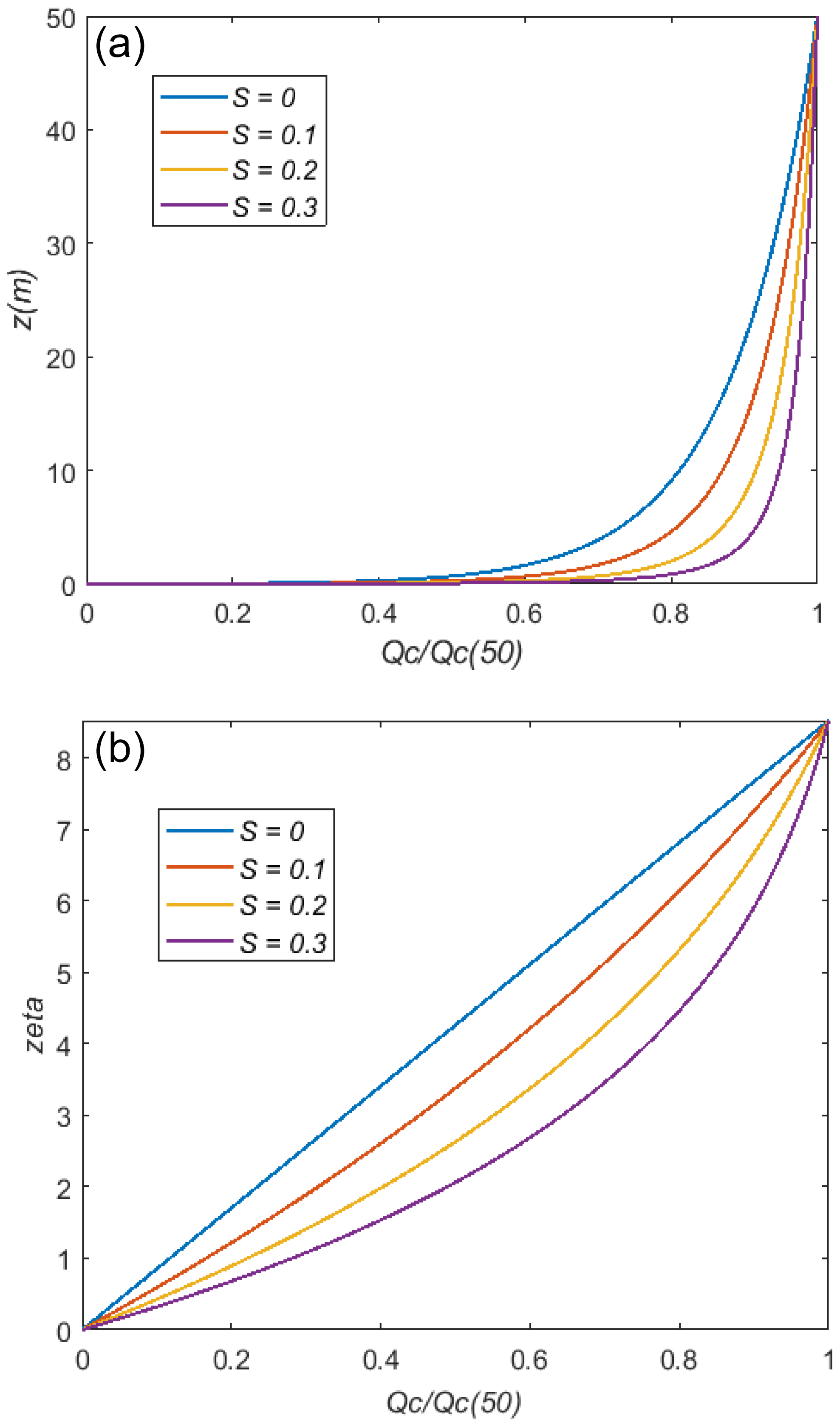
Figure 1 Qc profiles, scaled by the 50 m value, from the surface to z=50 m in constant flux layers with gravitational settling. The surface roughness length for aerosol removal z_0c is 0.01 m. Plotted with linear (a) and logarithmic (b) height scales and four S values.

Sample V_dep results are shown in Fig. 2 when V_g≥0. In the first case (a) we took $z_{\mathrm{0}\mathrm{m}}=z_{\mathrm{0}\mathrm{c}}=\mathrm{0}$.01 m so that R_s=0. With no gravitational settling both models agree. For S>0, the CFLGS deposition velocities (Eq. 15) are lower than those computed from the Zhang–Slinn formulation. Cases (b) and (c) keep z_0m at 0.01 m but allow z_0c to be smaller, R_s>0 in (b), or larger, R_s < 0 in (c). The CFLGS relationship (Eq. 15) always shows a modest V_dep reduction, relative to the Zhang–Slinn equation, which is typically of the order of 20 %.

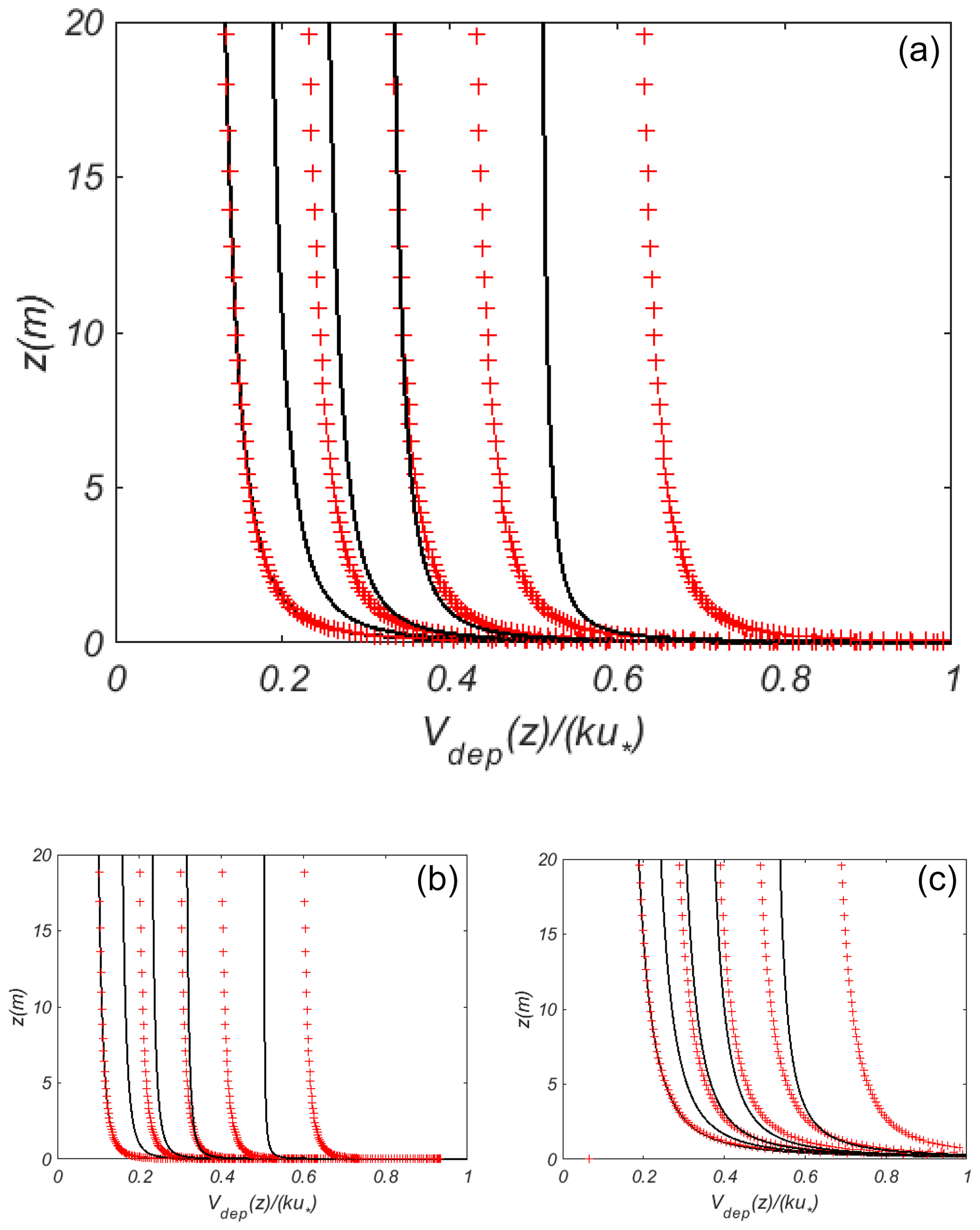
Figure 2 V_dep profiles, from the surface to z=20 m in constant flux layers with gravitational settling. Solid lines are with the CFLGS model, the + points are from the Zhang–Slinn formulation (ZS). The five cases, left to right, are S=0, S=0.1, S=0.2, S=0.3 and S=0.5. (a) $z_{\mathrm{0}\mathrm{m}}=z_{\mathrm{0}\mathrm{c}}=\mathrm{0}$.01 m; R_s=0. (b) z_0c=0.001 m; z_0m=0.01 m; $k{u}_{*}{R}_{\mathrm{s}}=\mathrm{2}$.3. (c) z_0c=0.1 m; z_0m=0.01 m; $k{u}_{*}{R}_{\mathrm{s}}=-\mathrm{2}$.3.

Another way to look at the relative importance of gravitational settling for these uniformly sized droplets is to consider the relative contributions to the total downward flux of aerosol ($u_{*}{q}_{c*}$). The gravitational contribution is simply V_gQc, while the turbulent diffusion contribution is

$$\begin{array}{}\text{(16)}& k{u}_{*}\mathrm{dQc}/\mathrm{d}\mathit{\zeta }=u_{*}{q}_{c*}{e}^{-S\mathit{\zeta }},\text{where}\mathit{\zeta }=\ln \left(\right(z+z_{\mathrm{0}\mathrm{c}})/z_{\mathrm{0}\mathrm{c}}).\end{array}$$

The ratios of turbulent transfer (TT) $/$ total flux and gravitational settling (GS) $/$ total flux then become

$$\begin{array}{}\text{(17)}& \mathrm{TT}=e^{-S\mathit{\zeta }}\text{and}\mathrm{GS}=\mathrm{1}-e^{-S\mathit{\zeta }}.\end{array}$$

Noting that $\mathit{\zeta }=\ln \left(\right(z+z_{\mathrm{0}\mathrm{c}})/z_{\mathrm{0}\mathrm{c}})$, we can see that these ratios depend on both z_0c, through the z(ζ) relationship, and S and will vary with z. Figure 3 illustrates this. It is important to note that Fig. 3 is based on z_0c=0.01 m. If we increase this to z_0c=0.1 m, then turbulent fluxes become more important (Fig. 2c). We can see that the TT ratio is formally 1 at the surface, where Qc = 0, so there is no gravitational component. For very large ζ values the TT term would decay to 0, but this would be well above the constant-flux-layer approximation. At 50 m the value will depend on S and z_0c.

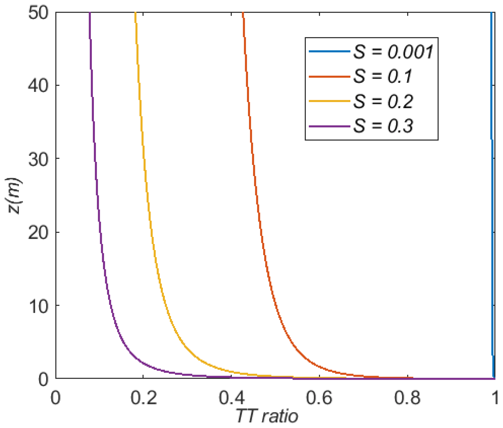
Figure 3 Variation in the turbulent transfer fraction of the total Qc flux and its variation with z and S. Note that these z values are based on z_0c=0.01 m.

4 Stable stratification case

For fog applications over land, radiation fog often occurs at low wind speeds with stable stratification. Advection fog when warm, moist air is advected over a colder surface is another case with stable stratification. For constant flux boundary layers in these circumstances, MOST gives, for velocity, $K_m=k(z+z_{\mathrm{0}\mathrm{m}})/{\mathrm{\Phi }}_M(z/L)$ and

$$\begin{array}{}\text{(18)}& \begin{array}{rl}{\mathrm{\Phi }}_M(z/L)& =\mathrm{1}+\mathit{\beta }(z+z_{\mathrm{0}\mathrm{m}})/L\\ U& =(u_{*}/k)\left(\ln \right((z+z_{\mathrm{0}\mathrm{m}})/z_{\mathrm{0}\mathrm{m}})+\mathit{\beta }z/L).\end{array}\end{array}$$

Observed profiles give β=5 (Garratt, 1992, p. 52). In addition Φ_H=Φ_M, and if we extend this idea to ${\mathrm{\Phi }}_{\mathrm{Qc}}(z/L)$ and set K_Qc to $k(z+z_{\mathrm{0}\mathrm{c}})/{\mathrm{\Phi }}_{\mathrm{Qc}}(z/L)$, we need to solve

$$\begin{array}{}\text{(19)}& \begin{array}{rl}& V_{\mathrm{g}}\mathrm{Qc}+\left[k{u}_{*}\right(z+z_{\mathrm{0}\mathrm{c}})/{\mathrm{\Phi }}_{\mathrm{Qc}}(z/L\left)\right]\mathrm{dQc}/\mathrm{d}z\\ & =F_{\mathrm{Qc}}=u_{*}{q}_{c*}\end{array}\end{array}$$

or, with ${\mathrm{\Phi }}_{\mathrm{Qc}}(z/L)=\mathrm{1}+\mathit{\beta }(z+z_{\mathrm{0}\mathrm{c}})/L,$

$$\begin{array}{ll}{\displaystyle }& {\displaystyle }\mathrm{dQc}/\mathrm{d}z+S\mathit{\left\{}\right(\mathrm{1}+\mathit{\beta }(z+z_{\mathrm{0}\mathrm{c}})/L)/(z+z_{\mathrm{0}\mathrm{c}}\left)\mathit{\right\}}\mathrm{Qc}\\ {\displaystyle }& {\displaystyle }=(q_{c*}/k)(\mathrm{1}+\mathit{\beta }(z+z_{\mathrm{0}\mathrm{c}})/L)/(z+z_{\mathrm{0}\mathrm{c}}),\text{with}S=V_{\mathrm{g}}/\left(k{u}_{*}\right).\end{array}$$

The integrating factor is $\exp (\int S(\mathrm{1}/(z+z_{\mathrm{0}\mathrm{c}})+\mathit{\beta }/L)\mathrm{d}z=(z+z_{\mathrm{0}\mathrm{c}}{)}^S\exp (S\mathit{\beta }z/L)$ so that

$$\begin{array}{ll}{\displaystyle }& {\displaystyle }\mathrm{d}\left[\right(z+z_{\mathrm{0}\mathrm{c}}{)}^S\exp (S\mathit{\beta }z/L)\mathrm{Qc}]/\mathrm{d}z\\ {\displaystyle }& {\displaystyle }=(q_{c*}/k)(\mathrm{1}+\mathit{\beta }(z+z_{\mathrm{0}\mathrm{c}})/L)(z+z_{\mathrm{0}\mathrm{c}}{)}^{S-\mathrm{1}}\exp (S\mathit{\beta }z/L),\end{array}$$

and we need to integrate the right-hand side. To do this it is convenient to let $\mathit{\beta }(z+z_{\mathrm{0}\mathrm{c}})/L=x$, and the integral that we need is of

$$\begin{array}{}\text{(20)}& {\displaystyle }\begin{array}{rl}& (q_{c*}/k)(L/\mathit{\beta }{)}^{S-\mathrm{1}}\exp (-S{x}_{\mathrm{0}}\left)\mathit{\right\{}(\mathrm{1}+x)x^{S-\mathrm{1}}\exp \left(Sx\right)\mathit{\}},\\ & \text{where}{x}_{\mathrm{0}}=\mathit{\beta }{z}_{\mathrm{0}\mathrm{c}}/L.\end{array}\end{array}$$

After some guidance and a few trials, one can see that $\mathrm{d}/\mathrm{d}x\mathit{\left\{}{x}^S\exp \right(Sx\left)\mathit{\right\}}=(S{x}^{S-\mathrm{1}}+S{x}^S)\exp \left(Sx\right)$ and the integral required is simply $F(x,S)=x^S\exp \left(Sx\right)/S$. We then evaluate F(x,S) at $z=\mathrm{0},x=\mathit{\beta }{z}_{\mathrm{0}\mathrm{c}}/L$ and any other z values to allow us to plot Qc profiles. With stable stratification and light winds, the constant-flux approximation would only apply to a relatively shallow layer, so we normalize with Qc(ztop) and set ztop to 20 m in these cases. If Qc = 0 at z=0, we then have

$$\begin{array}{}\text{(21)}& \begin{array}{rl}\mathrm{Qc}\left(z\right)=& (q_{c*}/k)(L/\mathit{\beta }{)}^{-\mathrm{1}}\exp (S{x}_{\mathrm{0}}\left)\right[\exp (-Sx)x^{-S}\left)\right]\\ & \left[F\right(x,S)-F(x_{\mathrm{0}},S\left)\right],\end{array}\end{array}$$

and we can then plot the ratio Qc(z) $/$ Qc(ztop) as in Fig. 4. For S=0, with no gravitational settling, the profile will be essentially the same as the velocity profile in Eq. (18) above; i.e.

$$\begin{array}{}\text{(22)}& \mathrm{Qc}\left(z\right)=(q_{c*}/k)\left(\ln \right((z+z_{\mathrm{0}\mathrm{c}})/z_{\mathrm{0}\mathrm{c}})+\mathit{\beta }z/L).\end{array}$$

In addition to z_0c and S the key parameter is the Obukhov length, $L=-\mathit{\rho }{c}_p{u}_{*}^{\mathrm{3}}\mathit{\theta }/\left(kgH\right)$ (>0). Neutral stratification corresponds to L→∞, while stable stratification relationships (H < 0; L>0) are generally limited to $\mathrm{0}<z/L$ < 1. If we are concerned with height ranges up to 10 or 20 m, then L=10 m would be considered a very low value perhaps with $u_{*}\approx \mathrm{0}$.13 m s⁻¹ and $H\approx -\mathrm{20}$ W m⁻² as possible values. Figure 4 shows Qc(z) $/$ Qc(20 m) profiles in a typical case with our standard value of z_0c=0.01 m. We set L to 20 m and use a range of S values. For large droplets, S=0.4, Qc flux is dominated by gravitational settling and reductions in Qc towards 0 only occur in the lowest few metres. For smaller particles, S=0, S=0.01 and S=0.1, turbulent mixing dominates the deposition process. Note that the S=0 points (log + linear profiles) and the S=0.01 line almost overlap as one confirmation of the solution form.

Figure 4 Qc $/$ Qc(ztop) profiles with stable stratification, assuming ${\mathrm{\Phi }}_{\mathrm{Qc}}(z/L)=\mathrm{1}+\mathit{\beta }(z+z_{\mathrm{0}\mathrm{c}})/L$. We set β=5, L=20 m and z_0c=0.01 m.

In unstable stratification it is generally accepted that ${\mathrm{\Phi }}_H(z/L)\ne {\mathrm{\Phi }}_M(z/L)$, and relatively little is known about stability effects on the diffusion of other scalars. For aerosol Jia et al. (2021) assume Φ_Qc=Φ_H in unstable stratification but have proposed a new form, different from Φ_H, for Φ_Qc in stably stratified boundary layers. These are all based on the Richardson number. In principle one could numerically solve Eq. (19) for any suitable ${\mathrm{\Phi }}_{\mathrm{Qc}}(z/L)$ form, but our interest is primarily the stable case, and it is convenient that an analytic solution can be found for the generally accepted $\mathrm{\Phi }(z/L)$ forms if we assume Φ_Qc=Φ_H. Strictly speaking our $\mathrm{\Phi }(z/L)$ functions should be $\mathrm{\Phi }\left(\right(z+z_{\mathrm{0}})/L)$ functions, but we are generally dealing with z≫z₀, and it is customary to ignore that difference.

5 Conclusions

The initial idea behind this analysis was that, in marine fog, cloud droplets can both fall towards the underlying surface through gravitational settling and be diffused towards the surface by turbulence, and on contact they can coalesce with an underlying water surface. Taylor et al. (2021) apply these ideas to fog modelling with the WRF (Weather Research and Forecasting) model. During reviews of that work and an earlier version of the current paper, it became clear that some reviewers were reluctant to accept that turbulence could cause fog droplets to collide and coalesce with an underlying surface and even more reluctant to see this as a constant-flux-layer situation. Fog droplets are perhaps a special case, but the CFLGS concept is equally applicable to aerosol particles or droplets in general, provided that they are inert and without sources or sinks in the air. Desert dusts, various pollutants or micro-plastic fragments being blown out over lakes or the sea from sources on land may be examples. Here we could anticipate a situation with initial mixing through a relatively deep atmospheric layer over land being advected over an aerosol-capturing water surface, so one could envisage a situation over the water with a constant downward flux of aerosol due to gravitational settling plus turbulent diffusion in a low-level constant flux layer.

One implication of the CFLGS model is that simply adding gravitational settling (V_g) to a deposition velocity (V_dep) based on aerodynamic and surface resistances may overestimate the combined effects. If we use the CFLGS model, it can indicate reductions of the order of 20 %. These are small compared to the uncertainties based on deposition velocity measurements but may well be worth considering.