the Creative Commons Attribution 4.0 License.
the Creative Commons Attribution 4.0 License.
 | 15 Dec 2021
Why is the city's responsibility for its air pollution often underestimated? A focus on PM2.5
Philippe Thunis
Alain Clappier
Alexander de Meij
Enrico Pisoni
Bertrand Bessagnet
Leonor Tarrason
While the burden caused by air pollution in urban areas is well documented, the origin of this pollution and therefore the responsibility of the urban areas in generating this pollution are still a subject of scientific discussion. Source apportionment represents a useful technique to quantify the city's responsibility, but the approaches and applications are not harmonized and therefore not comparable, resulting in confusing and sometimes contradicting interpretations. In this work, we analyse how different source apportionment approaches apply to the urban scale and how their building elements and parameters are defined and set. We discuss in particular the options available in terms of indicator, receptor, source, and methodology. We show that different choices for these options lead to very large differences in terms of outcome. For the 150 large EU cities selected in our study, different choices made for the indicator, the receptor, and the source each lead to an average difference of a factor of 2 in terms of city contribution. We also show that temporal- and spatial-averaging processes applied to the air quality indicator, especially when diverging source apportionments are aggregated into a single number, lead to the favouring of strategies that target background sources while occulting actions that would be efficient in the city centre. We stress that methodological choices and assumptions most often lead to a systematic and important underestimation of the city's responsibility, with important implications. Indeed, if cities are seen as a minor actor, plans will target the background as a priority at the expense of potentially effective local actions.
- Article
(2056 KB) - Full-text XML
- BibTeX
- EndNote


About 55 % of the world's population lives in urban areas nowadays, and this number is expected to increase to 68 % by 2050, according to the United Nations (UN2018, 2018). Large population growth is also projected by 2030 in most of the major European cities (Alberti et al., 2019), with predicted population growth varying between Berlin (15 %), Paris (19 %), Milan and Rome (21 %), Prague (37 %), London (39 %), and Brussels (52 %) (see https://urban.jrc.ec.europa.eu/thefutureofcities/urbanisation#the-chapter, last access: 24 November 2021). As a result of this population trend, urban emissions and their associated pollution levels are expected to increase as well.
According to a recent estimate (EEA, 2020), about 74 % of the EU-28 urban population is exposed to pollution of fine particulate matter (PM2.5) in concentrations above the WHO air quality guidelines value; this number rises to 99 % for ozone (O3) and is about 4 % for nitrogen dioxide (NO2). Air pollution is a heavy burden on human health, with more than 380 000 premature deaths in the EU-28 reported in 2017 according to the same EEA estimates. For a wide range of European cities, Khomenko et al. (2021) showed that the health burden due to air pollution varies greatly by city, with annual premature mortality reaching up to 15 % for PM2.5 and 7 % for NO2. The highest mortality burden for PM2.5 occurs in northern Italy, southern Poland, and eastern Czech Republic. De Bruyn and de Vries (2020) showed that for all 432 cities in their sample (total population: 130 million inhabitants), the social costs (e.g. hospital admissions, premature mortality) but also the costs due to air pollution exceeded EUR 166 billion in 2018 for Europe (EU-27 plus the UK, Norway, and Switzerland). City size was shown to be a key factor contributing to the total social costs: all cities with a population over 1 million feature in the top 25 cities with the highest social costs due to air pollution.
Given the health and economic burden caused by air pollution in urban areas, it is important to identify the origin of this pollution in order to reduce and control its impact. Identifying the sources of urban pollution and then assigning responsibilities enables a process to implement measures and control air pollution. Assessing the responsibility or share of cities for their pollution has important implications. For being effective, pollution reduction plans must be designed and applied to target the most polluting sectors at the relevant spatial scale (national, regional, and/or local) and with the appropriate temporal scales. In this context, quantifying the share of the city pollution caused by their own emissions becomes a crucial element to determine whether actions need to be applied locally or at the regional, national, or continental scale. This has important governance consequences for the effective control of air pollution.
For pollutants like NO2 that mostly originate from traffic sources and have a relatively short lifetime in the atmosphere, there is a general agreement on the fact that cities are the main contributor to these pollutant concentration levels and that acting locally on traffic emissions is the most efficient way of improving NO2 concentration levels in a particular city (Tobías et al., 2020). There is available European-wide information, such as in Degraeuwe et al. (2019), providing overviews of the potential impact of traffic emission reductions per vehicle type in different European cities. There is also agreement regarding O3 that this secondary pollutant is most effectively reduced by implementing reduction measures at larger spatial scales, involving actions driven at the regional and even continental scales (e.g. Luo et al., 2020). For other pollutants, like PM2.5, complex physical and chemical atmospheric processes with different timescales drive its formation, involving numerous precursors themselves emitted by several sources. The sources of PM2.5 pollution range from local traffic, domestic fuel burning, and industrial activities to regional sources such as agriculture in rural areas. Even though the latter emissions do not originate from cities, Thunis et al. (2018) showed that their impact on urban pollution could be important, reaching up to 30 % in several European cities. Because of this complexity, there is less consensus regarding a city's responsibility for or share of its pollution when addressing PM2.5. Because of this lack of consensus and the major burden of PM2.5 on health, we focus our analysis on this pollutant.
The usual approach to assess the city's share of pollution levels (in other words the city's responsibility) is source apportionment (SA). However, many SA approaches exist. The most widely used SA methods are the “potential impact” (or brute force), “increment”, and “tagging” approaches. An overview description of these methods and an evaluation of their limitations and capabilities for use can be found in Thunis et al. (2019). Moreover, many ways to parameterize them exist as well, leading to a variety of results and interpretations. For the 18 million inhabitants of New Delhi, Amann et al. (2017) concluded that only 40 % of the PM2.5 pollution was originating from local city sources, based on potential impact SA and expressed in terms of city-averaged population exposure, averaged yearly. In the context of the Copernicus programme, CAMS (Copernicus Atmosphere Monitoring Service) performs SA calculations daily with two different approaches, namely tagging and potential impacts, for a series of European cities. Results show important differences on a day-by-day basis, although these differences smooth out when considering longer-term averages (Pommier et al., 2020). Based on the increment approach, Kiesewetter and Amann (2014) derived SA estimates for a series of European cities and aggregated these detailed results at the country level, leading to relatively low city responsibilities (e.g. about 25 % for French, German, and Italian cities). Based on a potential impact approach, Thunis et al. (2018) estimated city shares for 150 cities in Europe. They highlighted their large variability across Europe and stressed the importance of the definition of the city with regards to the results by testing the sensitivity to different city extensions. The choice of the SA method, but also the way this method is configured, can lead to very different outcomes for the city's share of pollution, ranging from cities being a major contributor to their pollution to cities having a limited responsibility. This explains why the actual city's responsibility for its pollution remains a topic of discussion and why some authors stress the importance of local actions (Thunis et al., 2018; Wu et al., 2011; Raifman et al., 2020) when others stress the need for regional, national, or even continental actions (Huszar et al., 2016; ApSimon et al., 2021; Liu et al., 2013). This diversity of conclusions has serious consequences in terms of policy decisions. Blaming external (i.e. outside the city) pollution sources as being primarily responsible for urban pollution is sometimes an easy argumentation for decision makers to justify local inaction.
This work aims at explaining the main causes of discrepancies between different assessments of the city emission's impact on its pollution levels and show that these discrepancies generally lead to underestimation of the city's responsibility. It proposes a specific harmonized nomenclature for source apportionment approaches, and it shows how it is important to document the choices to enable correct interpretation of the results. We begin with a conceptual overview of the parameters structuring any SA approach (Sect. 2). This includes the definition of the key parameters of any SA study: indicator, source, receptor, and methodology to relate them. Then (Sect. 3) we assess the sensitivity of the urban SA results to the choices of these four parameters. In Sect. 4, we analyse implications in terms of air quality planning and suggested strategies. We finally provide conclusions in Sect. 5.
In this section, we detail the steps required to quantify the responsibility of a city for its air pollution through source apportionment (SA). SA is a methodology that serves to estimate the contribution of a given source at a specific receptor for a given indicator (for example the concentration of a given pollutant like PM or NO2). It involves the following steps (Fig. 1):
-
defining a relevant indicator, denoted as (I) to characterize air pollution;
-
defining the receptor (R) through its spatio-temporal characteristics, i.e. the area () and time period () over which the indicator is averaged;
-
defining the source (S), in our case the city, and its spatio-temporal characteristics, i.e. the city area (xs) and time period for which the city's responsibility is assessed (ts);
-
selecting the source apportionment (SA) methodology to capture the processes that relate the source to the receptor.
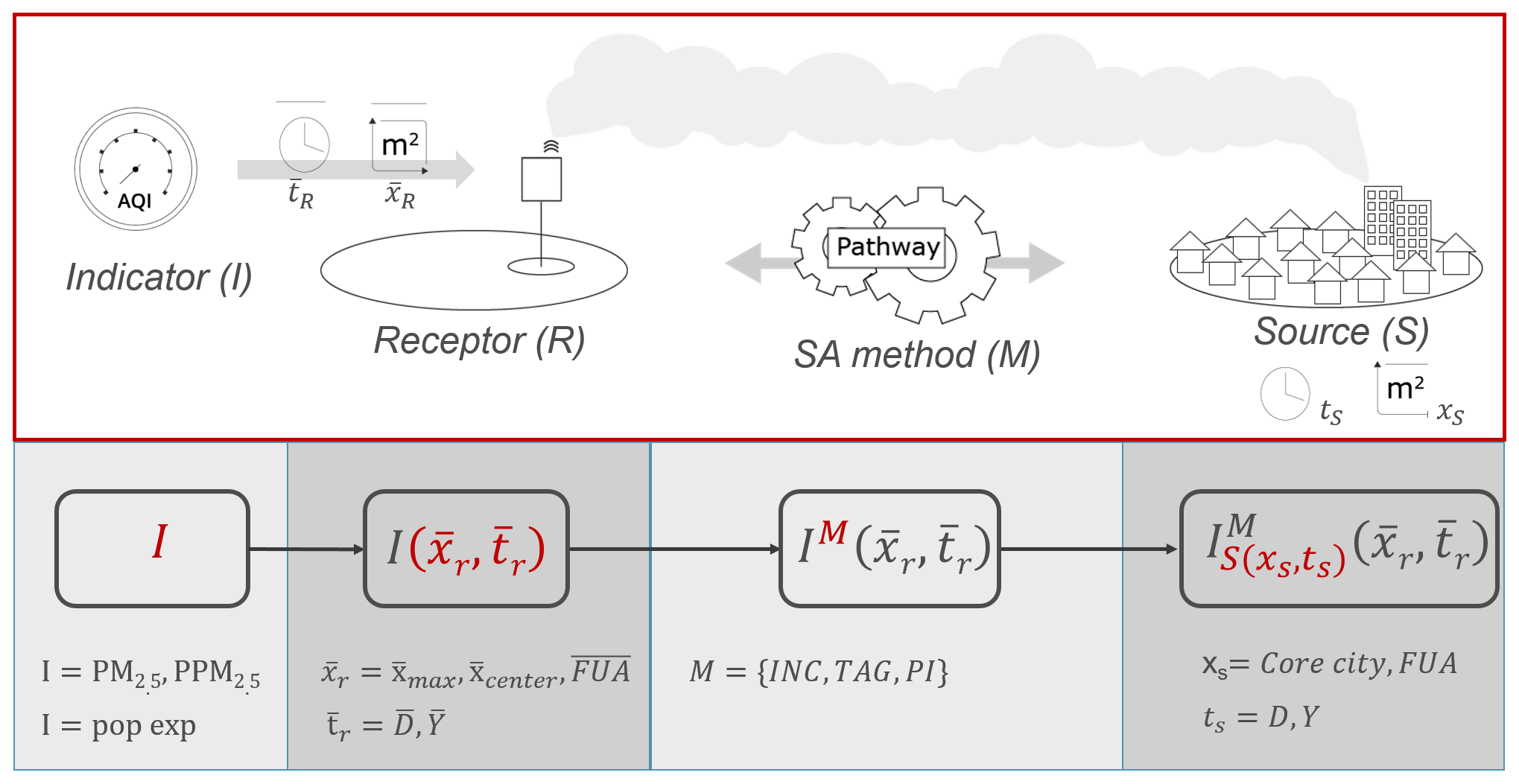
Figure 1Schematic flow chart representing the four steps required to fully define any SA process. The red letters indicate the indicator characteristic under consideration. The general notation for the indicator (I) includes a superscript for the methodological approach (M), a subscript to inform about the source (S), and brackets to inform about the receptor (R). The spatial and temporal dimensions associated with the source and receptor are denoted by “x” and “t”, respectively. The overbar indicates an averaging process. The lowest row provides for each parameter examples used in this work. Some images used in this schematic flow chart are adapted from https://www.flaticon.com/ (last access: 24 November 2021).
Figure 1 summarizes these steps as well as the nomenclature and symbols used in this work. We use this new nomenclature to attach contextual information (i.e. metadata) to the source apportionment. Further explanations of the symbols are given in the subsections below.
2.1 Definition of the air pollution indicator (I)
The first step required to assess the role and responsibility of city emissions with respect to its air pollution is to define an indicator that identifies the pollution aspect we are interested in. The indicator can be defined in many ways, for example as the total concentration of a given compound (e.g. PM), as a specific constituent of that total concentration (e.g. PM2.5 or its primary fraction, PPM), as a composite based on a mix of different pollutants (e.g. maximum among O3, PM2.5, and NO2 concentrations as in some air quality indexes such as ATMO2003, 2003), or as population exposure (i.e. product of population and concentration).
2.2 Definition of the receptor (R)
Estimating the indicator, from either a measuring instrument or a model simulation, implies an averaging process in both space and time. For model data, averages correspond to the spatial and temporal resolutions (e.g. the time step and grid cell size), whereas for measurement, the space–time average will depend on the instrument acquisition time and on the atmospheric dispersion characteristics at the measuring site. Regardless of these intrinsic time and space averages, indicators are generally averaged over longer spatial and temporal scales for convenience. The receptor is defined as the spatio-temporal entity over which the indicator is averaged. Both a spatial and a temporal scale (denoted by and , respectively) must be associated with the receptor to define it.
For the temporal dimension, typical examples for PM2.5 are days () or years (). Spatially, the indicator can be estimated at a specific location, e.g. the city centre () or at the location where the maximum concentration occurs (), or it can be averaged over the city (). For convenience, we use interchangeably the following notations to refer to the receptor:
2.3 Definition of the source (S)
The source is defined as the spatio-temporal entity (e.g. city, emission macro-sector, etc.) for which we assess the contribution to the indicator. For the purpose of this work, the source is defined as the city and more precisely as the emissions that originate from it. The source emissions (denoted by E) are indeed responsible for the pollution fraction that can be associated with the source or city at the receptor (R). These emissions are characterized by a spatial (xs = extension of the city) and a temporal scale (ts = period of time over which the source activity is assessed). For convenience, we use interchangeably the following notations to refer to the source:
In this work, we analyse in particular the impact of the city extension (xs) on the apportionment outcome. For this purpose, we define cities in two ways:
-
as core cities, i.e. the local administrative units, with a population density above 1500 km−2 and a population above 50 000, where the majority of the population lives in an urban centre, and
-
as functional urban areas (OECD, 2012, denoted as “FUAs”) composed of core cities plus their wider commuting zone, consisting of the surrounding travel-to-work areas where at least 15 % of the employed residents work in the city.
Details on the FUA and core city areas are available for 150 EU cities in the urban PM2.5 atlas (Thunis et al., 2017). Note that other city definitions exist. In the context of the CAMS source allocation analysis, cities are defined as an arbitrary number of grid cells in the modelling domain (Pommier et al., 2020).
Finally, we define the city background as the sum of all contributions from sources that are not covered by the spatial (xs) and temporal (ts) scales of the city source.
One main difference between sources and receptors is that for the latter, spatio-temporal characteristics are averaged. Apart from this, temporal and spatial characteristics can also differ in terms of value. For example, the source can be defined as the FUA (xs = FUA), while the receptor is a specific location (). Temporally, interest can be in assessing the contribution of the city weekly activity (ts = 1 week) for a given day () at the receptor. In the results presented here, the source and receptor temporal scales are however chosen to be identical for convenience.
2.4 Selection of the SA methodology
When the air pollution indicator and the spatio-temporal characteristics of both the receptor and the source have been selected, the next step consists of distinguishing and quantifying the fractions of the indicator related to the city source (Icity(R)) and to the background (Ibg(R)) at the receptor R, respectively. This decomposition is summarized by the following equation:
Different SA methodologies exist to perform this operation. In this section, we describe three main approaches, but only in brief, as details about each of these are discussed in other works (Clappier et al., 2017; Thunis et al., 2019, 2018; Mertens et al., 2018). As mentioned previously, we use the indicator's superscript to refer to its calculation method (). Methods are summarized in Table 1.
-
Potential impacts (PI). The city contribution in this method is denoted as and is calculated as the difference between two simulations: a base case that includes the city (I(R)) and a scenario in which the city emissions are switched off . In this notation, the source superscript (here, 100) indicates the percentage intensity by which the source emissions are reduced. Reductions are intended as percentage variations from the base case situation. The same approach can be used with reduction percentages that are lower than 100 %. In this case the resulting difference is divided by the reduction percentage to obtain the potential impact . A similar approach is used to calculate the background contribution, i.e. by removing or reducing partially the background emission sources. Potential impact methods for source apportionment are widely used (Osada et al., 2009; Huszar et al., 2016; Huang et al., 2018; Wang et al., 2014, 2015; Van Dingenen et al., 2018; Thunis et al., 2016; Clappier et al., 2015; Pisoni et al., 2017).
-
Increment (INC). With this methodology, the background contribution is estimated as the concentration observed or modelled at a given location “y” . This location must be far enough from the source to not feel its influence but be close enough to the source to avoid influences from other sources external to the city. These assumptions are further described and discussed in Thunis et al. (2017). The city contribution is then obtained as the difference between the base case indicator and the background contribution . The increment methodology has been used by, for example, Lenschow et al. (2001), Petetin et al. (2014), Kiesewetter et al. (2015), Squizzato and Masiol (2015), Timmermans et al. (2013), Keuken et al. (2013), Ortiz and Friedrich (2013), and Pey et al. (2010).
-
Tagging (TAG). With this approach, species emitted by the city are numerically tagged and followed through the modelled transport, dispersion, and chemical transformation processes. When chemical transformations take place, preserved atoms are used as tracers. For example, the nitrogen atom (N) will be used to follow the NO source emissions through its successive transformations into NO2 and HNO3 to reach its final product NO3, which will then be attributed to that source. Example of tagging applications are, for example, Kranenburg et al. (2013), Yarwood et al. (2004), Wagstrom et al. (2008), Kwok et al. (2013), Bhave et al. (2007), and Wang et al. (2009). Some of these approaches are implemented operationally to estimate daily city contributions to air pollution (https://topas.tno.nl/documentation/, last access: 24 November 2021). The formulations corresponding to these three main approaches are summarized in Table 1.
Table 1Formulation of the three main methods to estimate the contribution, potential impact, and increment of a city. The letters, I, S, and R refer to the indicator, source, and receptor, respectively. The indicator superscript refers to the SA method (PI for potential impacts, INC for increments, and TAG for tagging), while its subscript indicates the source (city or background (bg)); α represents the percentage reduction factor applied for the source emissions in the potential impacts method. See text for additional details.

A few key points are worth noting. While tagging and potential impact approaches explicitly consider city emissions in their calculations, this is not the case for increments that only refer to them implicitly. By construction, both the increment and tagging approaches are additive (i.e. ), whereas this is not the case for potential impacts when pollutants behave non-linearly because of air transport, deposition, or chemical processes (Clappier et al., 2017).
Recognizing the impossibility of assessing the sensitivity of the results for all combinations of indicators, source, receptor, and methodology, we focus our analysis on comparisons in which only one parameter is changed at a time to highlight major sensitivities. For this purpose, we use the following two main sources of data and results.
-
SHERPA. SHERPA is a modelling tool based on source–receptor relationships that represent a simplified version of a chemistry transport model, used to simulate the contribution to PM2.5 concentration levels by all precursor emissions (NOx, non-methane volatile organic compounds (NMVOCs), PPM, SO2, and NH3) from different cities in Europe (Clappier et al., 2015; Thunis et al., 2016, 2018). In its current configuration, SHERPA is based on the CHIMERE model (Menut et al., 2013) covering the whole of Europe at roughly 7 km spatial resolution. In this work, we use the source apportionment results over 150 cities as reported in the PM2.5 urban atlas (Thunis et al., 2017) as well as additional SHERPA data to provide further analysis.
-
EMEP simulations. The EMEP model is an offline regional transport chemistry model (Simpson et al., 2012; https://github.com/metno/emep-ctm, last access: 24 November 2021). The model has 20 vertical levels, with the first level around 50 m. The model uses meteorological initial conditions and lateral boundary conditions from the European Centre for Medium-Range Weather Forecasts (ECMWF) Integrated Forecasting System (IFS). The meteorological year is 2015. Detailed information on the meteorological driver, land cover, model physics, and chemistry is described in Simpson et al. (2012) and in the EMEP 2017 status report (EMEP2017, 2017). In this work, we use specific simulations where emissions have been removed partially or fully in a series of European cities. Additional details regarding these simulations are provided together with the discussion of the results.
Based on these sources of information and data, we discuss hereafter the sensitivity of the SA results to the choice of the indicator (Sect. 3.1), to the choice of the methodology (Sect. 3.2), to the source (Sect. 3.3), and finally to the receptor (Sect. 3.4).
3.1 Sensitivity to the indicator
The implications resulting from the choice of the indicator are illustrated in Fig. 2 for four indicators based on SHERPA results for 150 cities in Europe. The four indicators selected to characterize air pollution are (a) the PM2.5 concentration (top left; from Thunis et al., 2017), (b) the anthropogenic fraction of PM2.5 (“PM2.5 ant”; top right), (c) the primary anthropogenic fraction of PM2.5 (“PPM2.5 ant”; bottom left), and (d) the primary fraction of PM2.5 originating from the transport and residential sectors (“PPM2.5 oxy”; bottom left). The reference (PM2.5 total mass; top left) corresponds to the indicator currently used in legislation (e.g. European Ambient Air Quality Directive, AAQD2008, 2008) against which health impacts are correlated (WHO2005, 2005). In the second case, the indicator is limited to its anthropogenic fraction (PM25 ant), excluding therefore natural contributions (dust, marine salt, etc.). This is motivated by the fact that policies have no impact on this component. According to this indicator, city contributions increase significantly (by about 20 % on average), and in some cities where natural dust pollution is important (e.g. in Sicily), the city's responsibility shifts from minor to major. If we further restrict the indicator to its primary anthropogenic fraction (“PPM2.5 ant”; bottom right) because of its suggested higher health burden (Park et al., 2018; Viana et al., 2008), the city contribution then increases significantly in most cities. This becomes even more striking if we limit the indicator to the PPM2.5 fraction originating from the transport and residential sectors (bottom right). These two sectors have recently been shown to generate the largest burden on human health given the high oxidative potential of their emissions (Daellenbach et al., 2020; Li et al., 2016). With this indicator, the majority of EU cities become main contributors to their pollution. Regarding the latter indicator, it is important to note that although the increasing adoption of electric vehicles shows rather positive impacts on health (Choma et al., 2020), the remaining PM emissions from road traffic like tyres and brake and road wear emissions (Kole et al., 2017; Grigoratos and Martini, 2014; Ntziachristos and Boulter, 2019) will remain an issue. The calculation of various geochemical indices (enrichment factor, geo-accumulation index, pollution index, and potential ecological risk) also show that road dust is extremely enriched and contaminated by elements from tyre and brake wear (e.g. Sb, Sn, Cu, Bi, and Zn).
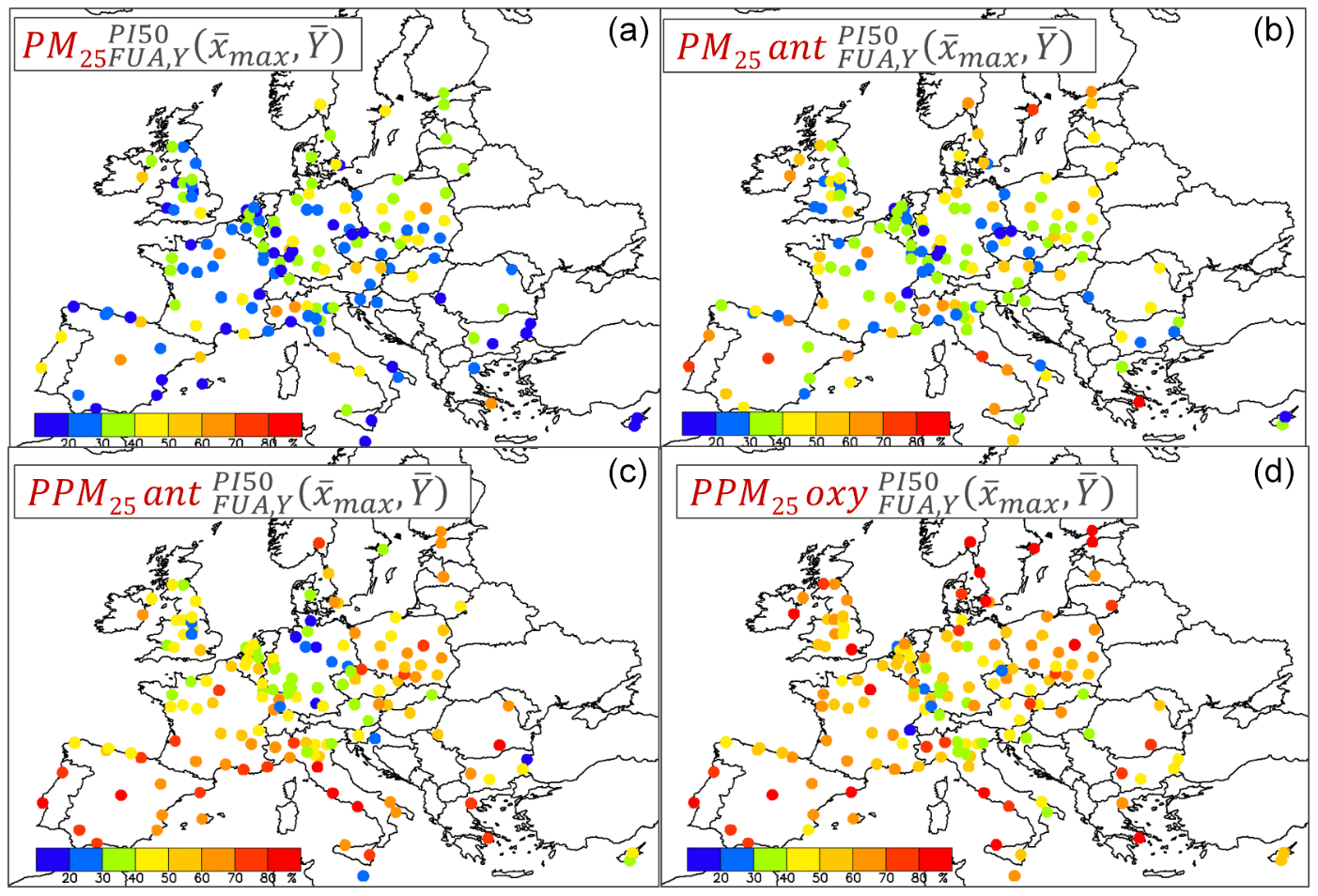
Figure 2SHERPA results for 150 major cities in Europe for the overall PM2.5 concentration (a), for its anthropogenic fraction (“PM25_ant”; b), for its anthropogenic primary fraction (“PPM25_ant”; d), and for its primary fraction originating from the transport and residential sectors (“PPM25_oxy”; c). For all cities, the source is defined spatially as the FUA over which emissions are reduced over a year (Y). The receptor is defined as the city location where the concentration is maximum (), and the indicator is averaged yearly at the receptor (). All calculations are made with the same SA methodology, namely potential impacts (PIs) with city emissions reduced by 50 % (PI50).
3.2 Sensitivity to the SA methodology
A comparison of SA methodologies is proposed in Thunis et al. (2019), where the potential impact, increment, and tagging approaches are compared on both simple theoretical examples and real data to highlight differences among methods and stress their limitations. In this section, we summarize the main findings of this work and complement it with comparisons that focus on the apportionment of the city vs. background contributions. We also provide in Appendix A a comparison of all SA methods discussed in this section, applied on a theoretical example tuned to the city scale.
3.2.1 Increment vs. potential impacts
Thunis (2018) compared increments and potential impacts with the SHERPA model for a series of European cities. He showed that increment approaches lead to important underestimations (30 % to 50 %) of the city's responsibility for PM2.5 and NO2 with respect to potential impacts. This underestimation is explained by the non-fulfilment of the two underlying increment assumptions related to the external location (i.e. y in ) being (1) far enough from the city to not feel its influence but (2) close enough to the city to avoid influences from sources external to the city. The authors show that these two assumptions are seldom fulfilled in reality.
3.2.2 Tagging vs. potential impacts
Clappier et al. (2017) discussed the concepts underlying these two SA methods and showed that important differences in terms of results arise as soon as non-linear processes are present. Belis et al. (2020) highlighted and quantified these large differences based on a real-case inter-comparison exercise. Finally, Thunis et al. (2019) reviewed in their work many inter-comparisons between tagging and potential impact SA results. In their application over the Po basin (Italy), they showed that differences are large for the agriculture sector (dominated by NH3 emissions) but are also important for other sectors when dealing with high temporal resolution (e.g. daily) at the receptor. Unfortunately, these examples did not address the particular case of a city-scale apportionment.
3.2.3 Full vs. partial potential impacts
To analyse differences between full and partial impacts, we use a series of EMEP simulations in which we remove totally (PI100) or partly (PI20) the London FUA emissions (source) during an entire year. Figure 3 shows the differences between city contributions obtained with the two PI methods. Differences can be important (up to 25 percentage points for specific days). Although the number of high-difference days is limited (leading to a yearly average difference of a few per cent), these days might represent high-pollution episodes for which assessing the city's responsibility is important to act. In general, the higher resolution applied to the temporal and/or spatial averages at the receptor, the larger the differences are among methods. It is also interesting to note that partial potential impacts systematically underestimate full potentials (no negative values).
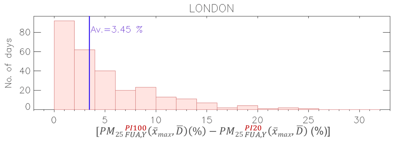
Figure 3Histogram of daily city contribution differences to London PM2.5 levels between two potential impacts methods, PI100 and PI20, calculated with the EMEP model. The source is defined spatially as the FUA where emissions are reduced yearly (Y subscript). The receptor is defined spatially as the city location where the maximum yearly averaged concentration is modelled () and temporally as daily average (). Each column represents the number of days with a specific PI difference (PI100 − PI20). The blue line provides the yearly average difference.
3.3 Sensitivity to the source
Figure 4 shows the comparison between SA obtained with sources defined as core cities (left) and as FUAs (right). The city contribution or responsibility is multiplied by a factor of 2 on average (see also Fig. 8) when FUAs are considered. The larger spatial extension of the FUA and its implied additional emissions explain the differences that lead some cities to become a major actor, i.e. where the city contribution dominates the background one (e.g. Athens, Warsaw, Milan, Turin, and Rome).

Figure 4Maps of city contributions obtained for spatial sources defined in two ways: core city (CC; a) and FUA (b). Results are shown for 150 cities in Europe based on the SHERPA-CHIMERE model using a potential impact SA method for a reduction strength of 50 % (PI50). The indicator is the total PM2.5 concentration. The receptor is selected as the location where the maximum yearly average concentration occurs () and applies a yearly time average (). The source emissions are reduced over a full year (Y).
3.4 Sensitivity to the receptor
In this section, we discuss the spatial and temporal averages applied at the receptor. Spatially, different averaging options exist, ranging from a single location (i.e. one model grid cell) to more or less extended areas covering part of the source or even larger. To illustrate the sensitivity of SA to that choice, we use the case of Paris (Fig. 5), where emissions have been reduced over the FUA (source) over a full year.
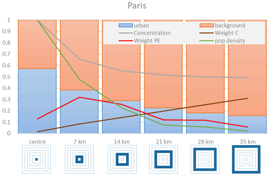
Figure 5City rings' source apportionment for Paris PM2.5 and associated population exposure. The city and background apportionment (bars) is represented for rings (i) progressively more distant from the city centre (x axis). The ring average concentration (Ci) and population density (Pi) relative to the city centre values are represented in blue and green, respectively. The relative (to the FUA total, i.e. all rings) weight of each ring (i) in the city average concentration (brown) is calculated as , where Si is the ring area. A similar expression () is used to determine the weight of each ring in the calculation of the average population exposure (red curve).
SA varies largely from one location to another within Paris. We highlight this with bars that distinguish the city vs. background contributions for locations at different distance from the city centre. We note opposite trends, dominated by the city source (around 60 %) at the city centre and dominated by the background source towards the periphery (around 80 %). While the SA at the city centre is representative of a single cell within the city, this is not the case for SA close to the periphery. This is highlighted by the city rings (below the x axis) that indicate the area of representativeness of a given SA. When we spatially average an indicator (PM2.5 or population exposure) over a receptor that covers the entire FUA (all six rings), these areas of representativeness enter into play. The brown curve indicates the weight (in the spatial average) attached to each city ring relative to the city total (i.e. all rings). Weights increase fast when moving towards the periphery because of the larger ring areas. The spatial-averaging process leads to over-representation of the periphery, which outweighs the city centre SA by almost a factor of 40. It is interesting and counterintuitive to note that with this averaging process, the city's responsibility decreases when the city area increases. With population exposure as an indicator (weights shown by the red curve), the rapid population density decrease balances the ring area increase when moving outward, leading to weights that dominate for middle rings. With average population exposure, the city centre weight is still similar to the weight obtained 28 km away.
Figure 6 compares SA for 150 cities obtained for receptors defined (1) as the location where the maximum concentration is reached within the FUA () and (2) as the FUA spatial average (). On average, city impacts for a spatially averaged receptor are about 55 % lower. Depending on the spatial characteristic of the receptor, some cities will be considered to be minor or major actors with respect to their pollution. We discuss this point further in Sect. 4.
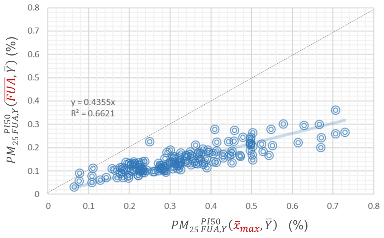
Figure 6Comparison of potential impacts for 150 cities in Europe obtained for a receptor spatially defined as the location where the concentration is maximum in the city ( – x axis) and defined as the spatially averaged FUA (). For these calculations, the source is defined as the FUA over which emissions are switched off during the whole year. The indicator is the total PM2.5 mass. All results are based on the SHERPA-CHIMERE model using a potential impact SA method for a reduction strength of 50 % (PI50) and are based on yearly averages at the receptor ().
As seen from these results, spatial averages at the receptor significantly reduce the city's responsibility, potentially leading to underestimation of the city's ability to reduce pollution levels via local controls. The large differences resulting from the choice of the receptor settings prevent meaningful comparisons. It is for example challenging to compare CAMS city contributions that are averaged spatially over the city area with the urban results obtained in the context of the Thematic Strategy on Air Pollution (Kiesewetter and Amann, 2014) that are aggregated at the country level or with SHERPA estimates based on a single grid cell receptor. It is therefore crucial to associate all SA settings (metadata) to the results in order to inform about the meaningfulness of a comparison. We further discuss this issue in the context of air quality planning in Sect. 4.
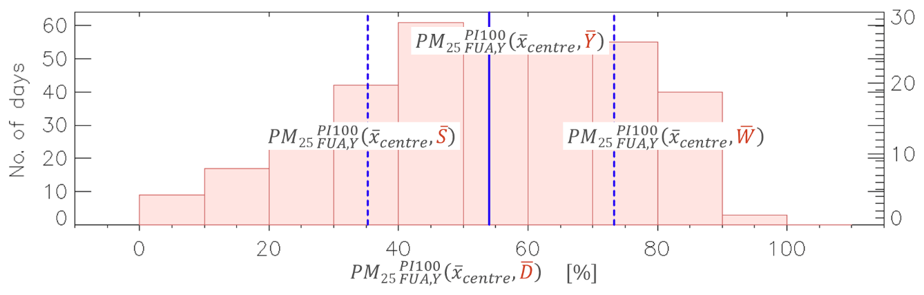
Figure 7Frequency histogram of daily potential impact at 100 % (PI100) modelled with the EMEP model for the city of Madrid. Each column represents the number of days with a given daily PI. The blue line provides the yearly average PI. For these calculations, the source is the Madrid functional urban area (FUA) over which emissions are switched off during the whole year (Y). The indicator is the total PM2.5 mass. The receptor point is the city centre location ().
Similar considerations apply to temporal averages. Figure 7 compares SA obtained when the indicator at the receptor is averaged yearly and seasonally with daily single values. For a yearly average, Madrid city's contribution is 54 %, but the spectra of daily contributions show variations that range from 10 % to beyond 90 %. Even seasonal averages show important differences of a factor of 2 between summer and winter. Similarly to spatial averages, temporal averages encompass a large spectra of SA outcomes. Indicators averaged yearly at the receptor have been used for example in SHERPA (Thunis et al., 2017) and GAINS (Kiesewetter and Amann, 2014), whereas daily indicators are used in CAMS (Pommier et al., 2020). Correlating low and high city contributions to meteorological factors (cold vs. warm days, windy vs. calm situations, etc.) is beyond the scope of this work. This point is however addressed in Pisoni et al. (2021).
Note that spatial averages have a larger smoothing effect than temporal ones because they are bidimensional.
3.5 Methodological assumptions and uncertainties
In addition to referring to the SA method itself (Sect. 2.4), other modelling parameters need to be documented as well. We list the main ones hereafter.
One of the main assumptions attached to models is the spatial resolution and its potential impact on the calculation of the city contribution. While a coarse resolution might be able to capture relatively well the background (characterized by smoother fields), this will not be the case for peak concentrations within the city. The coarser the model spatial resolution, the larger the underestimation of the city's responsibility will be (De Meij et al., 2007).
Uncertainties may result from our incomplete knowledge of some model input parameters, in particular chemical processes and emission sources. Some urban emission sources are not well documented and are probably underestimated. This is the case for residential emissions, for which the inclusion of condensable organic species remains a question mark (Bessagnet and Allemand, 2020; Simpson et al., 2020), or for the resuspension of particles generated by vehicles (Amato et al., 2014). On the other hand the spatial allocation for emissions can be uncertain for some sectors. These lacking or incomplete emission sources will lead to a potential misestimate of the city's responsibility.
On the meteorological side, the estimation of wind speed, planetary boundary layer (PBL) height, and/or turbulence intensity will largely influence the dispersion of city emissions and uncertainties, and these will therefore impact the calculation of city contributions. While the impact of meteorological parameterization on air quality has been extensively assessed from regional to urban cases (De Meij et al., 2009, 2015, 2018; Jiang et al., 2020), only few studies assessed their importance to city contributions. One of these (Huszar et al., 2021) shows, for example, that the inclusion of an urban canopy meteorological forcing in multi-year simulations largely impacts the estimation of the city's responsibility. In the next section, we discuss the consequences of these results on policy, in particular when SA information is used to design air quality plans.
Estimating a city's pollution contribution has important consequences in terms of air quality management. Indeed, an important city contribution will be a logic argument to support substantial control measures at the local level to abate pollution. The effectiveness of the control measures then relies on the relevance and accuracy of this city contribution; over- or underestimated city contributions potentially lead to inefficient measures.
In previous sections, we see that the city contribution largely varies depending on the choices made for the SA setting parameters (definition of the indicator, source, receptor, and methodology), hence the challenge to obtain a relevant and accurate estimate to support local action.
Given the range of possible SA options and their impact on results, the first recommendation is obviously to report these SA setting choices together with the results to provide policymakers with the full picture and allow them to take informed decisions. This advocates for the use of the proposed nomenclature or a similar one that reports and details the choices in the SA approach, providing accountability of the method and enabling correct interpretation of the results. The proposed nomenclature can be understood as a documentation of the SA metadata information. Apart from this point on the importance of documenting SA approach choices, we show below that some of the SA settings are fixed by the purpose of the study. We provide suggestions for the remaining free choices.
4.1 METHOD: an approach based on potential impacts is recommended for SA
It is important to recall that not all SA methodologies are equally suited to support air quality planning. As mentioned by several authors (Burr and Zhang, 2011; Qiao et al., 2018; Mertens et al., 2018; Clappier et al., 2017; Grewe et al., 2010, 2012; Thunis et al., 2019), potential impacts are recommended when non-linear species are involved (which is the case for PM2.5 and PM10 but also for other species like NO2 or O3). It is worth reminding that tagging or incremental approaches are still used erroneously and believed to be suited for air quality planning purposes (Qiao et al., 2018; Guo et al., 2017; Itahashi et al., 2017; Timmermans et al., 2017; Wang et al., 2015; Hendriks et al., 2013). Although challenging practical issues are attached to potential impacts and may be seen as a burden (e.g. lack of additivity; see Appendix), they only reflect the complexity of the real processes that must be accounted for. It is true that uncertainties associated with the PI approach (e.g. imperfect emission inventory) may lead other SA methods to perform better in some instances because methodological biases compensate uncertainties; this is however coincidental. While uncertainties can be tackled and reduced to improve the approach, this is not the case for methodological biases. These points are extensively discussed in Thunis et al. (2019).
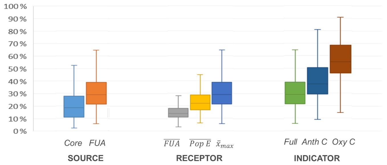
Figure 8Box quantile diagrams summarizing the city contributions to PM2.5 levels for the 150 EU cities. All results are based on a similar method (potential impacts at 50 %) and a similar temporal receptor () but for different choices of city sources (left), receptors (centre), and indicators (right). See previous sections for details. The two extremities of each vertical line represent the 10th and 90th percentile contributions among the 150 cities, respectively. The box crossing the horizontal line represents the median.
For the remainder of this section, focusing on policy aspects, only potential impact results are discussed. Fixing the methodology, however, still leaves free options in terms of indicator, receptor, and source. Figure 8 summarizes the variability in the SA results presented in the previous sections (i.e. Figs. 2, 4, and 6) to these free options. Differences in terms of the city's responsibility reach a factor of 2 on average for each of these remaining parameters, with much larger values for some cities.
4.2 INDICATOR: the indicator choice is driven by health and environmental objectives
The choice of the indicator is generally motivated by health or environmental considerations. Currently, the WHO guidelines (WHO2005, 2005) refer to the total PM2.5 mass as the indicator correlating best with health impacts. These guidelines (or the Ambient Air Quality Directive, AAQD, limit values) are then the logical and most relevant indicator choice among the options presented in Sect. 3.1 and shown in Fig. 2. As illustrated by Fig. 8, evolving knowledge of health-related pollution impacts (i.e. the increased toxicity of some PM2.5 constituents like those related to the traffic and residential activities) might, however, drive the choice towards more detailed indicators (e.g. PPM2.5), leading to an increased responsibility for the cities.
4.3 SOURCE: importance of matching sources with governance levels
Figure 8 shows that plans limited to city cores would be significantly less efficient than if applied at the FUA scale. On average over all cities, the efficiency decreases by a factor of 2, but larger differences occur in many cities. The source does not, however, represent a free choice in the context of policy practice. Indeed, authorities in charge of air quality (AQ) plans only have power to act on the area under their responsibility, which sets where measures apply. The same applies for the source temporal characteristic, fixed as the period of time during which measures apply. A good match between the SA settings and the temporal and spatial characteristics of the source is therefore important to provide meaningful support to policymakers.
4.4 RECEPTOR: drawbacks associated with spatial- and temporal-averaging processes at the receptor
As clearly shown in Fig. 5, spatial-averaging processes lead to a loss of information. In our example, a city-average-based SA would totally occult the city centre SA. It would lead to a strategy that mostly targets the background at the expense of the city centre, where the high concentration issues would not be solved. This is well illustrated by Amann et al. (2017), who analyse the responsibility of the city of New Delhi for its air pollution, both at a city centre hot spot receptor and in terms of city-average population exposure. In the first case, SA suggests acting on local sources, while in the second, SA suggests acting on regional sources. Spatial averaging drives the balance towards regional actions that will be less effective in solving the pollution issue at the city centre. The larger the city, the more important this shift will be. As illustrated by Fig. 8, there is a difference of more than a factor of 2 between city-averaged and hot spot indicators. Similar considerations apply to temporal averages. Figure 7 clearly shows that yearly average values hide the potential for effective local actions during wintertime and even more on specific days.
Averaging implies merging, into one single number, locations and time instants that are characterized by different and sometimes opposite SA. This may lead to strategies that will not be efficient everywhere all the time. Whenever the final objective is to reduce a temporally or/and spatially averaged indicator (e.g. average population exposure), strategies would gain in efficiency with the following process: (1) perform SA and hierarchize the raw (not averaged) SA results into homogeneous spatio-temporal clusters; (2) design strategies on the basis of these clusters; (3) assess the strategy efficiency against the averaged indicator. The key here is to design strategies for raw or clustered results rather than averaged ones to prevent information loss. Note that designing a unique strategy based on multiple SA results (point 2 above) does not necessarily complicate the analysis as these different SAs will likely suggest action for different sectors of activity that can be combined in the final strategy.
Although air quality has improved in Europe over the last decades, in great part thanks to effective measures and consistent EU-wide legislation, pollution hot spots still remain in many European cities. The extent to which city emissions are causing these elevated urban pollution levels is however still a subject of scientific discussion. This can be explained by the complex processes driving the formation of some pollutants like PM2.5, for which there is not a simple relationship between emissions and concentrations (in other words, local emissions do not always imply local responsibilities). Source apportionment represents a useful technique to quantify the city's responsibility, but the approaches and applications are however not harmonized and therefore not comparable, resulting in confusing and sometimes contradicting interpretations.
In this work, we analysed how different SA approaches apply to the urban scale and how their building elements and parameters are defined and set. We identified the possible settings associated with four key steps in SA: indicator, receptor, source, and methodology. We showed that different choices for these settings lead to very large differences in terms of results. On average over the 150 large European cities selected as examples, the choices made for the indicator, the receptor, and the source each lead to an average difference of a factor of 2 in terms of the city's responsibility. These various options and the large differences that result highlight the difficulty of comparing results from different studies and stress the need to document the SA approach with its related metadata associated with the key four steps.
This work advocates for the use of a harmonized nomenclature to support the comparability of SA approaches. We propose the use of indexes and sub-indexes attached to the four key steps in any SA approach in a harmonized way to uniquely document the approach and enable correct interpretation of the results. We believe that the adoption of this nomenclature will provide clarity to the scientific discussion on different results and enable the correct interpretation of the results for policy applications. Even though this is applied to the specific case of PM2.5, the concepts presented here can easily be generalized to other pollutants.
In the context of supporting urban air quality plans, the SA configuration and most setting parameters are driven by the purpose of the AQ plan itself and by its associated constraints. While environment- and/or health-related considerations guide the choice of the indicator, the spatio-temporal characteristics of the source are strongly correlated to governance aspects. In other words, the source characteristics should reflect the governance levels to facilitate interpretation. Finally, the recommended SA method should be based on “potential impacts” to prevent misleading interpretations in terms of expected AQ plan outcome.
At the receptor level, temporal- and spatial-averaging processes lead to a loss of information, especially when diverging SA results are aggregated into a single number. Averaging process, in particular spatial, often lead to the favouring of strategies that target background sources while neglecting actions that would be efficient at the city centre. In our 150-city example, the impact of spatial averaging leads to an average difference of a factor of 2 in terms of the city's responsibility. Results differ not only from one city to the other and from one location to another in a given city, they also differ through time. To cope with this variability, we recommend using non-averaged SA results for the design of AQ strategies. Once clustered in homogeneous spatio-temporal classes, these can serve to understand where and when actions are most efficient. When implemented, the efficiency of abatement measures can then be assessed via spatially and temporally averaged indicators (e.g. city-average population exposure).
The responsibility of a city to its pollution is obviously city-dependent. But even for a given city, SA studies using different approaches and parameter settings will deliver very different outcomes. It is important to note that on top of departure from the methodological recommendations listed above, additional uncertainties and assumptions will most often lead to a systematic and important underestimation of the city's responsibility. We showed that on average over 150 European cities, departures in terms of source, receptor, and indicator may each lead to an underestimation by a factor of 2. This comes with important implications: if cities are seen as a minor actor, plans will target the background as a priority at the expense of potentially effective local actions.
Future work will consist of comparing spatially or temporally averaged SA results with SA results that are clustered in homogeneous spatio-temporal classes and assess the implications in terms of AQ strategy.
To illustrate the differences among SA methods, we use here the theoretical example schematically represented in Fig. A1. A city source (in red) emits with a Gaussian dispersion profile both primary PM (PPM) and a gas-phase precursor (NOx). The background pollution (in blue) is composed of a mix of NOx, NH3, and PPM compounds. The various chemical reactions that take place are simplified here for convenience into a single reaction; 1 mol of NH3 reacts with 1 mol of NOx to create 1 mol of ammonium nitrate (), i.e. secondary PM (). We assume here that the external compounds involved in the reaction (X) are abundant and do not have a limiting effect on the formation of PM. While the city emissions (source) remain unchanged, we modify the relative importance of the three background compounds so that the background becomes in turn PPM-, NOx-, and NH3-dominated. The PM concentration at a given location “x” is given by
Based on the formulations provided in Table 1 and Eq. (4), the expressions to calculate the city and background components for the theoretical example presented above are detailed in Table A1. While these formulations are relatively straightforward for potential impacts and increments, it is more complex for the tagging method. The city tagging component is the sum of all PM species that are directly related to the city emissions. This includes PPM and NO3 that are related to the PPM and NOx city emissions, respectively. For the background component, it includes PPM, NOx, and also NH4 that is related to the NH3 emissions. Tagging allows the NOx and NH3 emitted compounds to be followed through their chemical processes and transformations until they create NO3 and NH4, respectively, that can be attributed to their respective sources. As NOx is emitted by both sources, the total NO3 must be fractionated and attributed to each single source. In our example, the NO3 fraction attributed to the city depends on the ratio of the available NOx precursor at the location of interest . A similar process is used to calculate the background component.

Figure A1Schematic representation of the theoretical example used to compare the three SA approaches. The city source (in red) emits NOx and PPM. The background (in blue, including other cities as well as rural sources) is composed of NOx, PPM, and NH3 in different relative proportions (indicated by the arrow). The “cc” and “bg” symbols represent the city centre receptor and the background location used for the increment approach, respectively.
This example is used to compare the increment (INC), tagging (TAG), and potential impact (PI) SA approaches.
Table A1Formulations for the potential impacts, increments, and tagging approach for the example presented in Fig. A1. The indicator for all methods and components is the total particulate matter mass (PM). The SA method is indicated as superscript (PIα, INC, or TAG), whereas the source (city or bg) is in subscript. The receptor is the city centre (cc), while the rural location selected for the increment approach is denoted by “bg”. For the tagging, the source subscript is also expressed directly as emissions (E) distinguishing each compound (within brackets).

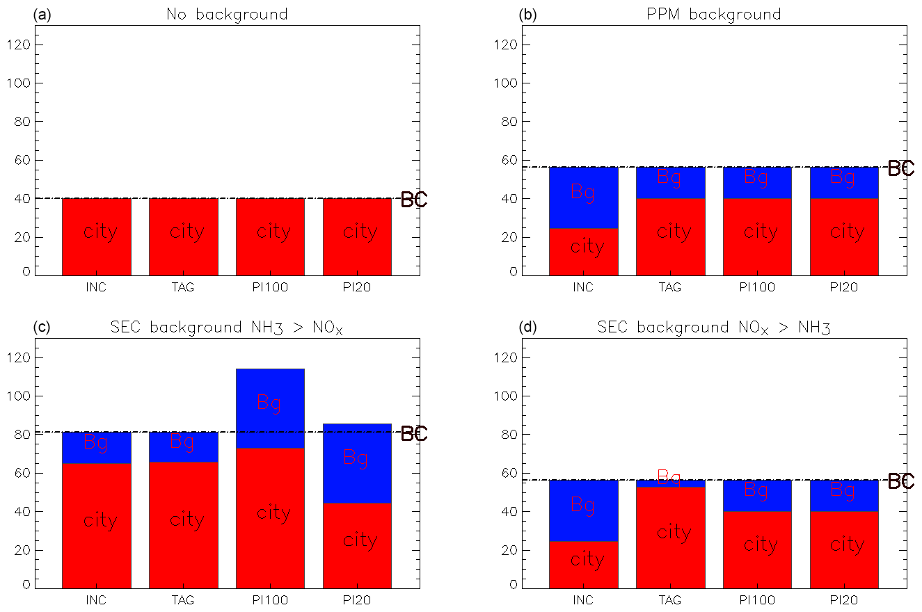
Figure A2Comparison of the city (red) and background (blue) components for four approaches applied to the theoretical examples described in Fig. A1. Results are expressed for different types of background: (a) no background, (b) background limited to PPM, (c) background limited to secondary but with NH3 > NOx, and (d) background limited to secondary but with NH3 < NOx.
Figure A2 shows the city and background contributions obtained with the three SA methods, differentiating two options for the PI one: 100 % (PI100) and 20 % reduction in the sources (PI20). The figure also distinguishes four situations characterized by different background compositions.
-
No background. When no background is present (top left), the city NOx emissions do not form PM, only PPM emissions do. In such cases, all methods deliver the same response.
-
PPM background. When the background is composed of PPM only (top right), no secondary species are formed. All methods agree, with the exception of the increment approach. This is due to the non-fulfilment of one of its underlying assumptions, i.e. the lack of spatial homogeneity of the background, which affects the rural and city locations differently (indicated by “cc” and “bg” in Fig. A2, respectively).
-
SEC background with NH3 > NOx. When secondary background precursors (NOx and NH3) reach the city (bottom row), SA methods deliver different results because they manage non-linear processes differently. When NH3 is more abundant than NOx (bottom left), the PI100 method does not preserve additivity (discussed in Sect. 2.4); i.e. the sum of the two components exceeds the total PM concentration. As seen from the results and also from Table A1, this is not the case for the increment and tagging approaches that are constructed to be additive.
-
SEC background with NH3 < NOx. When NH3 is less abundant than NOx (bottom right), differences remain important between the tagging, potential impact, and increment approaches, but additivity is preserved for both PI100 and PI10, which provide identical responses.
The SHERPA interface developed by the European Commission (EC-JRC) is available at https://aqm.jrc.ec.europa.eu/sherpa.aspx (last access: 24 November 2021), and its code is available at https://doi.org/10.5281/zenodo.5770956 (Pisoni, 2021a). The EMEP code developed by Met.No is available at https://github.com/metno/emep-ctm (Met.No, 2021).
The PM2.5 atlas data for 150 cities, produced by the European Commission (EC-JRC), are available at https://doi.org/10.5281/zenodo.5770975 (Pisoni, 2021b).
PT developed the methodological aspects and wrote most of the text. AC contributed to the methodological aspects and contributed to the writing on this. EP and AdM prepared data, including specific simulations, and contributed to the text. BB and LT reviewed and contributed to the text.
The contact author has declared that neither they nor their co-authors have any competing interests.
Publisher’s note: Copernicus Publications remains neutral with regard to jurisdictional claims in published maps and institutional affiliations.
The authors thank Chloé Thunis for her support in adapting some images from https://www.flaticon.com/ (last access: 24 November 2021) for our infographic needs.
This paper was edited by Eduardo Landulfo and reviewed by two anonymous referees.
AAQD2008: Directive 2008/50/EC of the European Parliament and of the Council of 21 May 2008 on ambient air quality and cleaner air for Europe, No. 152, Official Journal, Publications Office of the European Union, Luxembourg, 2008.
Alberti, V., Alonso Raposo, M., Attardo, C., Auteri, D., Ribeiro Barranco, R., Batista e Silva, F., Benczur, P., Bertoldi, P., Bono, F., Bussolari, I., Louro Caldeira, S., Carlsson, J., Christidis, P., Christodoulou, A., Ciuffo, B., Corrado, S., Fioretti, C., Galassi, M., Galbusera, L., Gawlik, B., Giusti, F., Gomez Prieto, J., Grosso, M., Martinho Guimaraes Pires Pereira, A., Jacobs, C., Kavalov, B., Kompil, M., Kucas, A., Kona, A., Lavalle, C., Leip, A., Lyons, L., Manca, A., Melchiorri, M., Monforti-Ferrario, F., Montalto, V., Mortara, B., Natale, F., Panella, F., Pasi, G., Perpia Castillo, C., Pertoldi, M., Pisoni, E., Roque Mendes Polvora, A., Rainoldi, A., Rembges, D., Rissola, G., Sala, S., Schade, S., Serra, N., Spirito, L., Tsakalidis, A., Schiavina, M., Tintori, G., Vaccari, L., Vandyck, T., Vanham, D., Van Heerden, S., Van Noordt, C., Vespe, M., Vetters, N., Vilahur Chiaraviglio, N., Vizcaino, M., Von Estorff, U., and Zulian, G., The Future of Cities, Vandecasteele, I., Baranzelli, C., Siragusa, A., and Aurambout, J. (Eds.): The future of cities, EUR 29752 EN, Publications Office of the European Union, Luxembourg, JRC116711, https://doi.org/10.2760/375209, 2019.
Amann, M., Purohit, P., Bhanarkar, A. D., Bertok, I., Borken-Kleefeld, J., Cofala, J., Heyes, C., Kiesewetter, G., Klimont, Z., Liu, J., Majumdar, D., Nguyen, B., Rafaj, P., Rao, P. S., Sander, R., Schöpp, W., Srivastava, A., and Vardhan, B. H.: Managing future air quality in megacities: A case study for Delhi, Atmos. Environ., 161, 99–111, 2017.
Amato, F., Cassee, F. R., Denier van der Gon, H. A. C., Gehrig, R., Gustafsson, M., Hafner, W., Harrison, R. M., Jozwicka, M., Kelly, F. J., Moreno, T., Prevot, A. S. H., Schaap, M., Sunyer, J., and Querol, X.: Urban air quality: The challenge of traffic non-exhaust emissions, J. Hazard. Mater., 275, 31–36, https://doi.org/10.1016/j.jhazmat.2014.04.053, 2014.
ApSimon, H., Oxley, T., Woodward, H., Mehlig, D., Dore, A., and Holland, M.: The UK Integrated Assessment Model for source apportionment and air pollution policy applications to PM2.5, Environ. Int., 153, 106515, https://doi.org/10.1016/j.envint.2021.106515, 2021.
ATMO2003: The ATMO index: an air quality indicator for developed areas in France, Eur. Ann. Allergy Clin. Immunol., 35, 166-9, available at: https://pubmed.ncbi.nlm.nih.gov/12838780/ (last access: 14 December 2021), 2003.
Belis, C. A., Pernigotti, D., Pirovano, G., Favez, O., Jaffrezo, J. L., Kuenen, J., Denier van Der Gon, H., Reizer, M., Riffault, V., Alleman, L. Y., Almeida, M., Amato, F., Angyal, A., Argyropoulos, G., Bande, S., Beslic, I., Besombes, J.-L., Bove, M. C., Brotto, P., Calori, G., Cesari, D., Colombi, C., Contini, D., De Gennaro, G., Di Gilio, A., Diapouli, E., El Haddad, I., Elbern, H., Eleftheriadis, K., Ferreira, J., Garcia Vivanco, M., Gilardoni, S., Golly, B., Hellebust, S., Hopke, P. K., Izadmanesh, Y., Jorquera, H., Krajsek, K., Kranenburg, R., Lazzeri, P., Lenartz, F., Lucarelli, F., Maciejewska, K., Manders, A., Manousakas, M., Masiol, M., Mircea, M., Mooibroek, D., Nava, S., Oliveira, D., Paglione, M., Pandolfi, M., Perrone, M., Petralia, E., Pietrodangelo, A., Pillon, S., Pokorna, P., Prati, P., Salameh, D., Samara, C., Samek, L., Saraga, D., Sauvage, S., Schaap, M., Scotto, F., Sega, K., Siour, G., Tauler, R., Valli, G., Vecchi, R., Venturini, E., Vestenius, M., Waked, A., and Yubero, E.: Evaluation of receptor and chemical transport models for PM10 source apportionment, Atmos. Environ., 5, 100053, https://doi.org/10.1016/j.aeaoa.2019.100053, 2020.
Bessagnet, B. and Allemand, N.: Review on Black Carbon (BC) and Polycyclic Aromatic Hydrocarbons (PAHs) emission reductions induced by PM emission abatement techniques (Informal document), Citepa – TFTEI Techno-Scientific Secretariat – UNECE, Paris, France, 2020.
Bhave, P. V., Pouliot, G. A., and Zheng, M.: Diagnostic model evaluation for carbonaceous PM2.5 using organic markers measured in the southeastern U.S., Environ. Sci. Technol., 41, 1577–1583, 2007.
Burr, M. J. and Zhang, Y.: Source apportionment of fine particulate matter over the Eastern U.S. Part II: source sensitivity simulations using CAMX/PSAT and comparisons with CMAQ source sensitivity simulations, Atmos. Pollut. Res., 2, 318–336, 2011.
Choma, E. F., Evans, J. S., Hammitt, J. K., Gómez-Ibáñez, J. A., and Spengler, J. D.: Assessing the health impacts of electric vehicles through air pollution in the United States, Environ. Int., 144, 106015, https://doi.org/10.1016/j.envint.2020.106015, 2020.
Clappier, A., Pisoni, E., and Thunis, P.: A new approach to design source–receptor relationships for air quality modelling, Environ. Model. Softw., 74, 66–74, 2015.
Clappier, A., Belis, C. A., Pernigotti, D., and Thunis, P.: Source apportionment and sensitivity analysis: two methodologies with two different purposes, Geosci. Model Dev., 10, 4245–4256, https://doi.org/10.5194/gmd-10-4245-2017, 2017.
Daellenbach, K. R., Uzu, G., Jiang, J., Cassagnes, L.E., Leni, Z., Vlachou, A., Stefenelli, G., Canonaco, F., Weber, S., Segers, A., Kuenen, J., Schaap, M., Favez, O., Albinet, A., Aksoyoglu, S. Dommen, J., Baltensperger, U., Geiser, M., Haddad, I., Jaffrezo, J. L., and Prévôt, A. S. H: Sources of particulate-matter air pollution and its oxidative potential in Europe, Nature, 587, 414–419, https://doi.org/10.1038/s41586-020-2902-8, 2020.
de Bruyn, S. and de Vries, J.: Health costs of air pollution in European cities and the linkage with transport, No. 20.190272.134, CE Delft, Delft, the Netherlands, 2020.
Degraeuwe, B., Pisoni, E., Peduzzi, E., De Meij, A., Monforti-Ferrario, F., Bodis, K., Mascherpa, A., Astorga-Llorens, M., Thunis, P., and Vignati, E.: Urban NO2 Atlas, EUR 29943 EN, Publications Office of the European Union, Luxembourg, JRC118193, https://doi.org/10.2760/43523, 2019.
De Meij, A., Wagner, S., Gobron, N., Thunis, P., Cuvelier, C., Dentener, F., and Schaap, M.: Model evaluation and scale issues in chemical and optical aerosol properties over the greater Milan area (Italy), for June 2001, Atmos. Res., 85, 243–267, 2007.
de Meij, A., Gzella, A., Cuvelier, C., Thunis, P., Bessagnet, B., Vinuesa, J. F., Menut, L., and Kelder, H. M.: The impact of MM5 and WRF meteorology over complex terrain on CHIMERE model calculations, Atmos. Chem. Phys., 9, 6611–6632, https://doi.org/10.5194/acp-9-6611-2009, 2009.
De Meij, A., Bossioli, E., Vinuesa, J. F., Penard, C., and Price, I.: The effect of SRTM and Corine Land Cover on calculated gas and PM10 concentrations in WRF-Chem, Atmos. Eniron., 101, 177–193, 2015.
De Meij, A., Zittis, G., and Christoudias, T.: On the uncertainties introduced by land cover data in high-resolution regional simulations, Meteorol. Atmos. Phys., 131, 1213–1223, https://doi.org/10.1007/s00703-018-0632-3, 2018.
EEA: Air Quality in Europe: 2020 Report, European Environment Agency, Publications Office, https://doi.org/10.2800/786656, 2020.
EMEP2017: Transboundary particulate matter, photo-oxidants, acidification and eutrophication components, Joint MSC-W & CCC & CEIP Report, EMEP Status Report 1/2017, Norwegian Meteorological Institute, Oslo, Norway, 2017.
Grewe, V., Tsati, E., and Hoor, P.: On the attribution of contributions of atmospheric trace gases to emissions in atmospheric model applications, Geosci. Model Dev., 3, 487–499, https://doi.org/10.5194/gmd-3-487-2010, 2010.
Grewe, V., Dahlmann, K., Matthes, S., and Steinbrecht, W.: Attributing ozone to NOx emissions: Implications for climate mitigation measures, Atmos. Environ., 59, 102–107, 2012.
Grigoratos, T. and Martini, G.: Non-exhaust traffic related emissions – Brake and tyre wear PM, EUR 26648g, Publications Office of the European Union, Luxembourg, JRC89231, https://doi.org/10.2790/22000, 2014.
Guo, H., Kota, S. H., Sahu, S. K., Hu, J., Ying, Q., Gao, A., and Zhang, H.: Source apportionment of PM2.5 in North India using source-oriented air quality models, Environ. Pollut., 231, 426–436, 2017.
Hendriks, C., Kranenburg, R., Kuenen, J., van Gijlswijk, R., Wichink Kruit, R., Segers, A., Denier van der Gon, H., and Schaap, M.: The origin of ambient particulate matter concentrations in the Netherlands, Atmos. Environ., 69, 289–303, https://doi.org/10.1016/j.atmosenv.2012.12.017, 2013.
Huang Y., Deng, T., Li, Z., Wang, N., Yin, C., Wang, S., and Fan, S.: Numerical simulations for the sources apportionment and control strategies of PM2.5 over Pearl River Delta, China, part I: Inventory and PM2.5 sources apportionment, Sci. Total Environ., 634, 1631–1644, 2018.
Huszar, P., Belda, M., and Halenka, T.: On the long-term impact of emissions from central European cities on regional air quality, Atmos. Chem. Phys., 16, 1331–1352, https://doi.org/10.5194/acp-16-1331-2016, 2016.
Huszar, P., Karlický, J., Marková, J., Nováková, T., Liaskoni, M., and Bartík, L.: The regional impact of urban emissions on air quality in Europe: the role of the urban canopy effects, Atmos. Chem. Phys., 21, 14309–14332, https://doi.org/10.5194/acp-21-14309-2021, 2021.
Itahashi, S., Hayami, H., Yumimoto, K., and Uno, I.: Chinese province-scale source apportionments for sulfate aerosol in 2005 evaluated by the tagged tracer method, Environ. Pollut., 220, 1366–1375, 2017.
Jiang, L., Bessagnet, B., Meleux, F., Tognet, F., and Couvidat, F.: Impact of physics parameterizations on high-resolution air quality simulations over the Paris region, Atmosphere, 11, 618, https://doi.org/10.3390/atmos11060618, 2020.
Keuken, M., Moerman, M., Voogt, M., Blom, M., Weijers, E. P., Röckmann, T., and Dusek, U.: Source contributions to PM2.5 and PM10 at an urban background and a street location, Atmos. Environ., 71, 26–35, 2013.
Khomenko, S., Cirach, M., Pereira-Barboza, E., Mueller, N., Barrera-Gómez, J., Rojas-Rueda, D., de Hoogh, K., Hoek, G., and Nieuwenhuijsen, M.: Premature mortality due to air pollution in European cities: a health impact assessment, Lancet Planetary Health, 3, S2542519620302722, https://doi.org/10.1016/S2542-5196(20)30272-2, 2021.
Kiesewetter, G. and Amann, M.: Urban PM2.5 levels under the EU Clean Air Policy Package, IIASA TSAP Report 12, IIASA, Vienna, Austria, 2014.
Kiesewetter, G., Borken-Kleefeld, J., Schöpp, W., Heyes, C., Thunis, P., Bessagnet, B., Terrenoire, E., Fagerli, H., Nyiri, A., and Amann, M.: Modelling street level PM10 concentrations across Europe: source apportionment and possible futures, Atmos. Chem. Phys., 15, 1539–1553, https://doi.org/10.5194/acp-15-1539-2015, 2015.
Kole, P. J., Löhr, A. J., Van Belleghem, F., and Ragas, A.: Wear and Tear of Tyres: A Stealthy Source of Microplastics in the Environment, Int. J. Env. Res. Pub. He., 14, 1265, https://doi.org/10.3390/ijerph14101265, 2017.
Kranenburg, R., Segers, A. J., Hendriks, C., and Schaap, M.: Source apportionment using LOTOS-EUROS: module description and evaluation, Geosci. Model Dev., 6, 721–733, https://doi.org/10.5194/gmd-6-721-2013, 2013.
Kwok, R. H. F., Napelenok, S. L., and Baker, K. R.: Implementation and evaluation of PM2.5 source contribution analysis in a photochemical model, Atmos. Environ., 80, 398–407, 2013.
Lenschow, P., Abraham, H.-J., Kutzner, K., Lutz, M., Preu, J.-D., and Reichenbacher, W.: Some ideas about the sources of PM10, Supplement No. 1, Atmos. Environ., 35, 23–33, 2001.
Li, Y., Henze, D. K., Jack, D., Henderson, B. H., and Kinney, P. L.: Assessing public health burden associated with exposure to ambient black carbon in the United States, Sci. Total Environ., 539, 515–525, 2016.
Liu, F., Klimont, Z., Zhang, Q., Cofala, J., Zhao, L., Huo, H., Nguyen, B., Schöpp, W., Sander, R., Zheng, B., Hong, C., He, K., Amann, M., and Heyes, C.: Integrating mitigation of air pollutants and greenhouse gases in Chinese cities: development of GAINS-City model for Beijing, J. Clean. Prod., 58, 25–33, https://doi.org/10.1016/j.jclepro.2013.03.024, 2013.
Luo, H., Yang, L., Yuan, Z., Zhao, K., Zhang, S., Duan, Y., Huang, R., and Fu, Q.: Synoptic condition-driven summertime ozone formation regime in Shanghai and the implication for dynamic ozone control strategies, Sci. Total Environ., 745, 141130, https://doi.org/10.1016/j.scitotenv.2020.141130, 2020.
Menut, L., Bessagnet, B., Khvorostyanov, D., Beekmann, M., Blond, N., Colette, A., Coll, I., Curci, G., Foret, G., Hodzic, A., Mailler, S., Meleux, F., Monge, J.-L., Pison, I., Siour, G., Turquety, S., Valari, M., Vautard, R., and Vivanco, M. G.: CHIMERE 2013: a model for regional atmospheric composition modelling, Geosci. Model Dev., 6, 981–1028, https://doi.org/10.5194/gmd-6-981-2013, 2013.
Mertens, M., Grewe, V., Rieger, V. S., and Jöckel, P.: Revisiting the contribution of land transport and shipping emissions to tropospheric ozone, Atmos. Chem. Phys., 18, 5567–5588, https://doi.org/10.5194/acp-18-5567-2018, 2018.
Met.No: EMEP code 4.34, GitHub [code], available at https://github.com/metno/emep-ctm, last access: 24 November 2021.
Ntziachristos, L. and Boulter, P.: EMEP/EEA air pollutant emission inventory guidebook 2019 – 1.A.3.b.vi Road transport: Automobile tyre and brake wear – 1.A.3.b.vii Road transport: Automobile road abrasion, European Environment Agency, Copenhagen, Denmark, 2019.
OECD: Redefining Urban: a new way to measure metropolitan areas, OECD report, Paris, France, ISBN 9789264174054, 148 pp., 2012.
Ortiz, S. and Friedrich, R.: A modelling approach for estimating background pollutant concentrations in urban areas, Atmos. Pollut. Res., 4, 147–156, https://doi.org/10.5094/APR.2013.015, 2013.
Osada, K., Ohara, T., Uno, I., Kido, M., and Iida, H.: Impact of Chinese anthropogenic emissions on submicrometer aerosol concentration at Mt. Tateyama, Japan, Atmos. Chem. Phys., 9, 9111–9120, https://doi.org/10.5194/acp-9-9111-2009, 2009.
Park, M., Joo, H. S., Lee, K., Jang, M., Kim, S. D., Kim, I., Borlaza, L. J. S., Lim, H., Shin, H., Chung, K. H., Choi, Y. H., Park, S. G., Bae, M. S., Lee, J., Song, H., and Park, K.: Differential toxicities of fine particulate matters from various sources, Sci. Rep., 8, 17007, https://doi.org/10.1038/s41598-018-35398-0, 2018.
Petetin, H., Beekmann, M., Sciare, J., Bressi, M., Rosso, A., Sanchez, O., and Ghersi, V.: A novel model evaluation approach focusing on local and advected contributions to urban PM2.5 levels – application to Paris, France, Geosci. Model Dev., 7, 1483–1505, https://doi.org/10.5194/gmd-7-1483-2014, 2014.
Pey, J., Querol, X., and Alastuey, A.: Discriminating the regional and urban contributions in the North-Western Mediterranean: PM levels and composition, Atmos. Environ., 44, 1587–1596, 2010.
Pisoni, E.: Why is the city's responsibility for its air pollution often underestimated? A focus on PM2:5, Zenodo [code], https://doi.org/10.5281/zenodo.5770956, 2021a.
Pisoni, E.: Why is the city's responsibility for its air pollution often underestimated? A focus on PM2:5, Zenodo [data set], https://doi.org/10.5281/zenodo.5770975, 2021b.
Pisoni, E., Clappier, A., Degraeuwe, B., and Thunis, P.: Adding spatial flexibility to source-receptor relationships for air quality modelling, Environ. Model. Softw., 90, 68–77, 2017.
Pisoni, E., Thunis, P., de Meij, A., and Bessagnet, B.: A new methodology to evaluate the effectiveness of local policies during high PM2.5 episodes: application on 10 European cities, submitted to Atmos. Chem. Phys., 2021.
Pommier, M., Fagerli, H., Schulz, M., Valdebenito, A., Kranenburg, R., and Schaap, M.: Prediction of source contributions to urban background PM10 concentrations in European cities: a case study for an episode in December 2016 using EMEP/MSC-W rv4.15 and LOTOS-EUROS v2.0 – Part 1: The country contributions, Geosci. Model Dev., 13, 1787–1807, https://doi.org/10.5194/gmd-13-1787-2020, 2020.
Qiao, X., Ying, Q., Li, X., Zhang, H., Hu, J., Tang, Y., and Chen, X.: Source apportionment of PM2.5 for 25 Chinese provincial capitals and municipalities using a source-oriented Community Multiscale Air Quality model, Sci. Total Environ., 612, 462–471, 2018.
Raifman, M., Russell, A. G., Skipper, T. N., and Kinney, P. L.: Quantifying the health impacts of eliminating air pollution emissions in the city of boston, Environ. Res. Lett., 15, 094017, https://doi.org/10.1088/1748-9326/ab842b, 2020.
Simpson, D., Benedictow, A., Berge, H., Bergström, R., Emberson, L. D., Fagerli, H., Flechard, C. R., Hayman, G. D., Gauss, M., Jonson, J. E., Jenkin, M. E., Nyíri, A., Richter, C., Semeena, V. S., Tsyro, S., Tuovinen, J.-P., Valdebenito, Á., and Wind, P.: The EMEP MSC-W chemical transport model – technical description, Atmos. Chem. Phys., 12, 7825–7865, https://doi.org/10.5194/acp-12-7825-2012, 2012.
Simpson, D., Fagerli, H., Colette, A., van der Gon, H. D., Dore, C., Hallquist, M., Hansson, H. C., Maas, R., Rouil, L., Allemand, N., Bergström, R., Bessagnet, B., Couvidat, F., Durif, M., Haddad, I. E., Safont, J. G., Grieshop, A., Fraboulet, I., Kausch, F., Hallquist, A., Hamilton, J., Juhrich, K., Klimont, Z., Kregar, Z., Mawdsely, I., Megaritis, A., Ntziachristos, L., Pandis, S., Prévôt, A. S. H., Schindlbacher, S., Seljeskog, M., Sirina-Leboine, N., Sommers, J., and Aström, S.: How should condensables be included in PM emission inventories reported to EMEP/CLRTAP? Report of the expert workshop on condensable organics organised by MSC-W, Gothenburg, 17–19 March 2020, EMEP Technical Report MSC-W 4/2020, Norwegian Meteorological Institute, 2020.
Squizzato, S. and Masiol, M.: Application of meteorology-based methods to determine local and external contributions to particulate matter pollution: A case study in Venice (Italy), Atmos. Environ., 119, 69–81, 2015.
Timmermans, R. M. A., Denier van der Gon, H. A. C., Kuenen, J. J. P., Segers, A. J., Honoré, C., Perrussel, O., Builtjes, P. J. H., and Schaap, M.: Quantification of the urban air pollution increment and its dependency on the use of down-scaled and bottom-up city emission inventories, Urban Climate, 6, 44–62, 2013.
Timmermans, R., Kranenburg, R., Manders, A., Hendriks, C., Segers, A., Dammers, E., Zhang, Q., Wang, L., Liu, Z., Zeng, L., Denier van der Gon, H., and Schaap, M.: Source apportionment of PM2.5 across China using LOTOS-EUROS, Atmos. Environ., 164, 370–386, 2017.
Thunis, P.: On the validity of the incremental approach to estimate the impact of cities on air quality, Atmos. Environ., 173, 210–222, 2018.
Thunis, P., Degraeuwe, B., Pisoni, E., Ferrari, F., Clappier, A., On the design and assessment of regional air quality plans: The SHERPA approach, J. Environ. Manage., 183, 952–958, https://doi.org/10.1016/j.jenvman.2016.09.049, 2016.
Thunis, P., Degraeuwe, B., Peduzzi, E., Pisoni, E., Trombetti, M., Vignati, E., Wilson, J., Belis, C., and Pernigotti, D.: Urban PM2.5 Atlas: Air Quality in European cities, EUR 28804 EN, Publications Office of the European Union, Luxembourg, JRC108595, https://doi.org/10.2760/336669, 2017.
Thunis, P., Degraeuwe, B., Pisoni, E., Trombetti, M., Peduzzi, E., Belis, C. A., Wilson, J., Clappier, A., and Vignati, E.: PM2.5 source allocation in European cities: A SHERPA modelling study, Atmos. Environ., 187, 93–106, 2018.
Thunis, P., Clappier, A., Tarrason, L., Cuvelier, C., Monteiro, A., Pisoni, E., Wesseling, J., Belis, C. A., Pirovano, G., Janssen, S., Guerreiro, C., and Peduzzi, E.: Source apportionment to support air quality planning: Strengths and weaknesses of existing approaches, Environ. Int., 130, 104825, https://doi.org/10.1016/j.envint.2019.05.019, 2019.
Tobías, A., Carnerero, C., Reche, C., Massagué, J., Via, M., Minguillón, M. C., Alastuey A., and Querol, X.: Changes in air quality during the lockdown in barcelona (spain) one month into the SARS-CoV-2 epidemic, Sci. Total Environ., 726, 138540, https://doi.org/10.1016/j.scitotenv.2020.138540, 2020.
UN2018: The World's Cities in 2018 – Data Booklet (ST/ESA/SER.A/417), United Nations, Department of Economic and Social Affairs, Population Division, New York, USA, 2018.
Van Dingenen, R., Dentener, F., Crippa, M., Leitao, J., Marmer, E., Rao, S., Solazzo, E., and Valentini, L.: TM5-FASST: a global atmospheric source–receptor model for rapid impact analysis of emission changes on air quality and short-lived climate pollutants, Atmos. Chem. Phys., 18, 16173–16211, https://doi.org/10.5194/acp-18-16173-2018, 2018.
Viana, M., Querol, X., Alastuey, A., Ballester, F., Llop, S., Esplugues, A., Fernandez-Patier, R., Garcia dos Santos, S., and Herce, M. D.: Characterising exposure to PM aerosols for an epidemiological study, Atmos. Environ., 42, 1552–1568, https://doi.org/10.1016/j.atmosenv.2007.10.087, 2008.
Wagstrom, K. M., Pandis, S. N., Yarwood, G., Wilson, G. M., and Morris, R. E.: Development and application of a computationally efficient particulate matter apportionment algorithm in a three dimensional chemical transport model, Atmos. Environ., 42, 5650–5659, 2008.
Wang, L., Wei, Z., Wei, W., Fu, J. S., Meng, C., and Ma, S.: Source apportionment of PM2.5 in top polluted cities in Hebei, China using the CMAQ model, Atmos. Environ., 122, 723–736, 2015.
Wang, L. T., Wei, Z., Yang, J., Zhang, Y., Zhang, F. F., Su, J., Meng, C. C., and Zhang, Q.: The 2013 severe haze over southern Hebei, China: model evaluation, source apportionment, and policy implications, Atmos. Chem. Phys., 14, 3151–3173, https://doi.org/10.5194/acp-14-3151-2014, 2014.
Wang, Z. S., Chien, C.-J., and Tonnesen, G. S.: Development of a tagged species source apportionment algorithm to characterize three-dimensional transport and transformation of precursors and secondary pollutants, J. Geophys. Res., 114, D21206, https://doi.org/10.1029/2008JD010846, 2009.
WHO2005: Air Quality Guidelines Global Update 2005. Particulate matter, ozone, nitrogen dioxide and sulfur dioxide, World Health Organisation, Geneva, Switzerland, ISBN 9289021926, 2005.
Wu, Q. Z., Wang, Z. F., Gbaguidi, A., Gao, C., Li, L. N., and Wang, W.: A numerical study of contributions to air pollution in Beijing during CAREBeijing-2006, Atmos. Chem. Phys., 11, 5997–6011, https://doi.org/10.5194/acp-11-5997-2011, 2011.
Yarwood, G., Morris, R. E., and Wilson, G. M.: Particulate Matter Source Apportionment Technology (PSAT) in the CAMx Photochemical Grid Model. Proceedings of the 27th NATO/CCMS International Technical Meeting on Air Pollution Modeling and Application, 24–29 October 2004, Banff, Alberta, Canada, Springer, Boston, MA, USA, 2004.