Measurement report: Characterization of the vertical distribution of airborne Pinus pollen in the atmosphere with lidar-derived profiles – a modeling case study in the region of Barcelona, NE Spain

This paper investigates the mechanisms involved in the dispersion, structure, and mixing in the vertical column of atmospheric pollen. The methodology used employs observations of pollen concentration obtained from Hirst samplers (we will refer to this as surface pollen) and vertical distribution (polarization-sensitive lidar), as well as nested numerical simulations with an atmospheric transport model and a simplified pollen module developed especially for this study. The study focuses on the predominant pollen type, Pinus, of the intense pollination event which occurred in the region of Barcelona, Catalonia, NE Spain, during 27–31 March 2015. First, conversion formulas are expressed to convert lidar-derived total backscatter coefficient and model-derived mass concentration into pollen grains concentration, the magnitude measured at the surface by means of aerobiological methods, and, for the first time ever, a relationship between optical and mass properties of atmospheric pollen through the estimation of the so-called specific extinction cross section is quantified in ambient conditions. Second, the model horizontal representativeness is assessed through a comparison between nested pollen simulations at 9, 3, and 1 km horizontal resolution and observed meteorological and aerobiological variables at seven sites around Catalonia. Finally, hourly observations of surface and column concentration in Barcelona are analyzed with the different numerical simulations at increasing horizontal resolution and varying sedimentation/deposition parameters. We find that the 9 or 3 km simulations are less sensitive to the meteorology errors; hence, they should be preferred for specific forecasting applications. The largest discrepancies between measured surface (Hirst) and column (lidar) concentrations occur during nighttime, where only residual pollen is detected in the column, whereas it is also present at the surface. The main reason is related to the lidar characteristics which have the lowest useful range bin at ∼ 225 m, above the usually very thin nocturnal stable boundary layer. At the hour of the day of maximum insolation, the pollen layer does not extend up to the top of the planetary boundary layer, according to the observations (lidar), probably because of gravity effects; however, the model simulates the pollen plume up to the top of the planetary boundary layer, resulting in an overestimation of the pollen load. Besides the large size and weight of Pinus grains, sedimentation/deposition processes have only a limited impact on the model vertical concentration in contrast to the emission processes. For further modeling research, emphasis is put on the accurate knowledge of plant/tree spatial distribution, density, and type, as well as on the establishment of reliable phenology functions.

1 Introduction

Pollen is a very important biological structure present all over the world. It functions as a container in which the male gametophyte generation of the angiosperms and gymnosperms is housed and is responsible of the gene flow. To be functional, mature pollen must be transported from the place where it is generated to the female structures of a flower of the same species, through a process named pollination. Several pollination types exist, with one of them being anemophily. Anemophily occurs when pollen grains are passively transported by the air. In this case, pollen behaves as biogenic aerosol and constitutes a substantial fraction of the mass of particulate matter in the air during the flowering season. Consequently, pollen can have strong health effects, causing allergenic rhinitis and asthma. The study of the pollen transport in the atmosphere is a relevant topic, not only because it allows the evaluation of the potential risks for human health and the prevention of its effects but also because it will possibly provide a better understanding of the spatial distribution of the species (Belmonte et al., 2008; Schmidt-Lebuhn et al., 2007; Sharma and Kanduri, 2007; Smouse et al., 2001).

Pinus is a dominant genus in the forested areas of the Northern Hemisphere, and this is also true in the region of Barcelona (Catalonia, NE Spain), which is the region of study for this work. Following the Catalan Ecological and Forestry Inventory (CEFI; Gracia et al., 2000–2004), 61 % (2×10⁶ ha) of the total surface of Catalonia is covered by forests, and Pinus (P. halepensis, P. nigra, P. pinaster, P. pinea, P. sylvestris, and P. uncinata) accounts for 39.2 % of this area. Because of the abundance of pines in the territory, their huge pollen production, and the pollen dispersion by anemophily, Pinus is one of the most abundant taxa in the atmospheric pollen spectra (Belmonte and Roure, 1991). Pinus pollen is in the top three of the most abundant pollen types in almost all stations of the Catalan Aerobiological Network (Xarxa Aerobiològica de Catalunya – XAC; https://aerobiologia.cat/pia/en/, last access: 1 December 2021). Although not considered an allergenic species, its abundance in the region makes this pollen type of interest to help understand the atmospheric transport processes affecting biological aerosols.

In the last few decades, several works have studied the transport of pollen species in the atmosphere, developed different numerical models, and compared the results with in situ surface observations. Such models include a source term and a dispersion module. The source term characterizes the pollen emission considering the start, end, and duration of the pollen season (e.g., Sofiev et al., 2013) and the diurnal profiles of the emission fluxes (e.g., Helbig et al., 2004; Sofiev et al., 2013) with parameterizations derived from statistical analysis of available observations (surface pollen counts and meteorological variables). The seminal works of Helbig et al. (2004), Schueler et al. (2005), Schueler and Schlünzen (2006), and Sofiev et al. (2006) showed the value of such models for studying the transport of pollen and their application as forecasting tools. Different models have been developed since then to model the transport of birch (Sofiev et al., 2006; Vogel et al., 2008; Efstathiou et al., 2011; Zink et al., 2013; Zhang et al., 2014), ragweed (Efstathiou et al., 2011; Zink et al., 2013; Prank et al., 2013; Wozniak and Steiner, 2017), grass (Zhang et al., 2014; Wozniak and Steiner, 2017), olive (Zhang et al., 2014; Sofiev et al., 2017), broadleaf tree pollen (Helbig et al., 2004; Wozniak and Steiner, 2017), and evergreen needleleaf tree pollen (Wozniak and Steiner, 2017) over regional domains, with horizontal resolutions ranging from 50 to 10 km. Although advancements in the field have been achieved, current models still present significant limitations to reproduce the life cycle of pollen, as highlighted in the model intercomparison works of Sofiev et al. (2015, 2017), where different transport models were used to study the pollination season of birch and olive with large variability among them. Nowadays, the Copernicus Atmosphere Monitoring Service (CAMS) regional production provides forecasts at the European continental scale of pollen concentration for birch, olive, grasses, ragweed, and alder using a multi-model ensemble approach (https://www.regional.atmosphere.copernicus.eu, last access: 1 December 2021). While the evaluation of these simulations is almost always performed against in situ pollen concentration measurements, nearly no information is known about their performance in the atmospheric column.

Scattering coupled to depolarizing properties, on the one hand, and emission of fluorescence spectra when excited with UV radiation of some chemical substances contained in pollen and bioparticles in general, on the other hand, are the two main properties of pollen grains that allow their remote detection in the atmospheric column with lidar techniques. The first property makes elastic, polarization-sensitive lidar systems powerful instruments for the detection of atmospheric pollen. The number of articles from the lidar community dealing with this topic has increased in recent years (Sassen, 2008; Noh et al., 2013; Sicard et al., 2016a; Bohlmann et al., 2019; Shang et al., 2020; Bohlmann et al., 2021). In particular, Shang et al. (2020) developed a method to retrieve the linear depolarization ratio of the pollen (or the mixture of pollen) present from measurements of the particle backscatter coefficient and depolarization ratio and Ångström exponent. The second property of pollen to emit characteristic fluorescence spectra has been known for a few years. Such spectra have been detected by the technique of the so-called laser-induced fluorescence lidars (Sugimoto et al., 2012; Sharma et al., 2015; Wojtanowski et al., 2015; Rao et al., 2017; Saito et al., 2018; Richardson et al., 2019). Very recently, fluorescence returns produced by atmospheric pollen excited at 355 nm were also measured with broadband filters and combined with multi-wavelength, multi-depolarization Raman retrievals (Veselovskii et al., 2020, 2021). Some authors even detected fluorescence effects of the aerosol of biogenic origin with the water vapor channel of an elastic/Raman lidar system (Immler et al., 2005). Although the use of lidar-derived, range-resolved information on the optical properties of pollen is available, it has never been used in a generalized manner for validating modeling experiments trying to reproduce the pollen release and transport in the atmosphere, nor has it been used as a complementary tool to understand the pollen vertical dispersion, distribution, and mixing. Some tentative exercises, published in reviewed proceedings of international conferences, using modeling to help understand the observed vertical distribution of Pinus and Platanus pollen from lidar observations in the region of Barcelona have been conducted by Sicard et al. (2016b, 2017, 2019). The present journal paper is the apogee of the knowledge presented during the latter three conference proceedings and has been acquired through a continuous effort since 2016.

The objective of the paper is to improve our understanding of pollen vertical distribution in the atmosphere by combining in situ concentration (Hirst), columnar optical property (lidar) measurements, and dispersion modeling. The paper is focused on the mechanisms responsible of the pollen vertical dispersion and mixing and how the pollen vertical structure impacts its horizontal transport. For that reason, the pollen type selected is Pinus, one of the most abundant (third position in the spectra of the period 1994–2020, after the ornamental species Platanus and Cupressaceae) in the region of Barcelona, our region of study. This work presents nested numerical simulations up to 1 km horizontal resolution of the dispersion of Pinus pollen in the atmosphere which occurred during a 5 d pollination event in the region of Barcelona during 27–31 March 2015 (Sicard et al., 2016a). The model evaluation in the atmospheric column is performed against continuous lidar measurements conducted in Barcelona. The results are discussed in terms of the pollen parametrization and the schemes used in the model. The present journal paper is the first one of its kind to study the vertical structure of a pollen species by means of nested numerical simulations.

2 Instrumentation

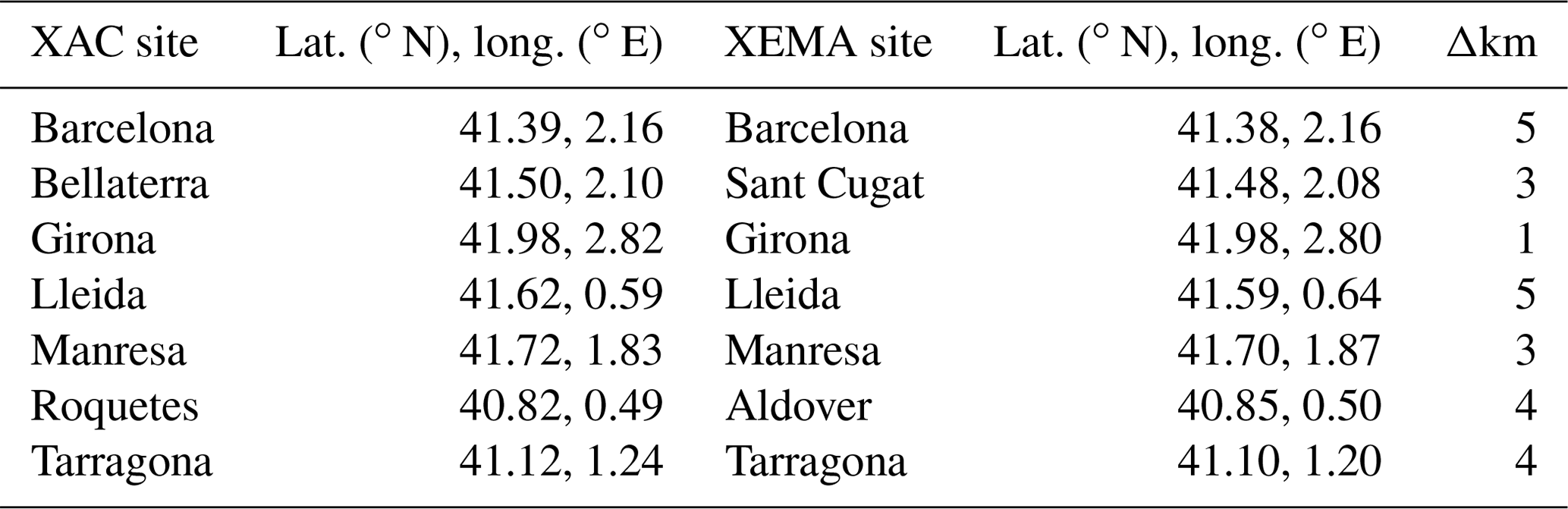
Pollen grain daily concentration was measured by the Aerobiological Network of Catalonia (Xarxa Aerobiològica de Catalunya – XAC) at seven sites around Catalonia (NE Spain). At the Barcelona site (2.165^∘ E, 41.394^∘ N; 67 m a.s.l. – above sea level) the pollen concentration was also measured at a time resolution of 1 h. The meteorology was taken from the seven nearest stations to the XAC sites of the Automatic Weather Stations Network (Xarxa d'Estacions Meteorològiques Automàtiques – XEMA; http://en.meteocat.gencat.cat/xema, last access: 1 December 2021) of the Meteorological Service of Catalonia (Meteocat). The coordinates of these stations are reported in Table 1, and their location is shown in Fig. 1a. Hourly profiles of particle backscatter coefficient and linear volume and particle depolarization ratios were acquired at the Remote Sensing Lab (RSLab) at the North Campus of the Universitat Politècnica de Catalunya (2.112^∘ E, 41.389^∘ N; 115 m a.s.l.), approximately 4.4 km to the west of the Barcelona XAC site.

2.1 Airborne pollen sampling

Pollen samples are obtained using volumetric suction pollen trap based on the impact principle (Hirst, 1952), the standardized method in European aerobiological networks (Galán et al., 2014). The Hirst sampler (Hirst, 1952) is calibrated to handle a flow of 10 L of air per minute, thus matching the human breathing rate. Pollen grains are impacted on a cylindrical drum covered by a Melinex film coated with silicon fluid (LANZONI srl^®) as trapping surface. The drum rotates at 2 mm per hour; so, each 48 mm represents 24 h of continuous sampling. The drum is changed weekly, and the exposed tape is cut into pieces, with each one corresponding to 1 d. Pollen grains are counted under a light microscope at 600× magnification. Daily average pollen counts are obtained following the standardized Spanish method (Galán et al., 2007), consisting of running four longitudinal sweeps along the 24 h slide for daily data and identifying and counting each pollen type found. To obtain the hourly concentrations, 24 continuous transversal sweeps separated every 2 mm along the daily sample slide are analyzed, since the drum rotates at a speed of 2 mm per hour. Daily and intra-diurnal (hourly) pollen concentrations are obtained by converting the pollen counts into particles per cubic meter of air, taking into account the proportion of the sample surface analyzed and the air intake of the Hirst pollen trap (10 L min⁻¹).

Table 1 Pollen (XAC) and meteorological (XEMA) surface stations used in this study. Δkm is the distance between XAC and XEMA stations.

2.2 Airborne pollen columnar measurements

The profiles of the particle backscatter coefficient and the volume and particle depolarization ratios were measured with the Barcelona micro-pulse lidar (MPL) system (Sigma Space Corporation; model MPL-4B). The system is part of the MPLNET (Micro-Pulse Lidar Network; http://mplnet.gsfc.nasa.gov/, last access: 1 December 2021; Welton et al., 2001) network. The MPL system is a compact, eye-safe lidar designed for full-time unattended operation (Campbell et al., 2002; Flynn et al., 2007; Welton et al., 2018). It uses a pulsed solid-state laser emitting low-energy pulses (∼ 6 µJ) at a high pulse rate (2500 Hz) and a co-axial transceiver design with a telescope shared by both transmit and receive optics. The Barcelona MPL optical layout uses an actively controlled liquid crystal retarder which makes the system capable of conducting polarization-sensitive measurements by alternating between two retardation states (Flynn et al., 2007). The signals acquired in each of these states are recorded separately and called “co-polar” and “cross-polar”. In a nominal operation, the raw temporal and vertical resolutions are 30 s and 15 m, respectively.

The total lidar signal, P_T, as a function of the altitude, z, is reconstructed from the co-polar, P_co, and cross-polar, P_cr, signals as follows (Flynn et al., 2007):

$$\begin{array}{}\text{(1)}& P_{\mathrm{T}}\left(z\right)=P_{\mathrm{co}}\left(z\right)+\mathrm{2}{P}_{\mathrm{cr}}\left(z\right).\end{array}$$

The particle backscatter coefficient, β^p, was retrieved with the two-component elastic algorithm (also known as the Klett–Fernald–Sasano method; Fernald, 1984; Sasano and Nakane, 1984; Klett, 1985), with a constant lidar ratio of 50 sr, and applied to the total lidar signal, P_T.

By adapting the notations of Flynn et al. (2007) to ours, one can formulate the linear volume depolarization ratio, δ^V, for the MPL system as follows:

$$\begin{array}{}\text{(2)}& {\mathit{\delta }}^{\mathrm{V}}\left(z\right)={\displaystyle \frac{P_{\mathrm{cr}}\left(z\right)}{P_{\mathrm{co}}\left(z\right)+P_{\mathrm{cr}}\left(z\right)}}.\end{array}$$

The linear particle depolarization ratio, δ^p, can then be determined by Eq. (4) of Sicard et al. (2016a). Finally, the extraction of the total pollen backscatter coefficient, β_pol, out of the particle backscatter coefficient is made thanks to the pollen depolarization capabilities (see Sicard et al., 2016a, and references therein).

We also calculated the vertical height, h_pol, up to which the pollen plume extends. As shown in Sicard et al. (2016a), the pollen plume is characterized during the entire pollination event by a near-constant or slightly decreasing profile of β_pol. From this aspect, the structure of the pollen plume is much simpler than the atmospheric boundary layer structure usually found in Barcelona (Sicard et al., 2006) and allows us to use a simple threshold method (Sicard et al., 2016a).

All the MPL retrievals presented in this work were performed with in-house algorithms and not with the MPLNET processing, since the system only entered the network in 2016.

3 Modeling

The dispersion of the airborne pollen in the atmosphere was modeled with the Multiscale Online Nonhydrostatic AtmospheRe CHemistry model (MONARCH; Pérez et al., 2011; Jorba et al., 2012; Badia and Jorba, 2015; Badia et al., 2017). The MONARCH model is a fully online multiscale chemical weather prediction system for regional and global-scale applications, with telescoping nest capabilities, developed at the Barcelona Supercomputing Center (BSC). The system is based on the meteorological Nonhydrostatic Multiscale Model on the B grid (NMMB; Janjic and Gall, 2012), widely verified at the National Centers for Environmental Prediction (NCEP). The MONARCH model couples online the NMMB with the gas-phase and aerosol continuity equations to solve the atmospheric chemistry processes in detail. The model is designed to account for the feedbacks among gases, aerosol particles, and meteorology. Currently, it can consider the direct radiative effect of aerosols while neglecting dynamic cloud–aerosol interactions. Different chemical processes were implemented following a modular operator splitting approach to solve the advection, diffusion, chemistry, dry and wet deposition, and emission of atmospheric constituents. Meteorological information is available at each time step to solve the chemistry. In order to maintain consistency with the meteorological solver, the chemical species are advected and mixed at the corresponding time step of the meteorological tracers, using the same numerical schemes implemented in the NMMB. The advection scheme is Eulerian, positive definite, and monotone, maintaining a consistent mass conservation of the chemical species within the domain of study (Janjic and Gall, 2012).

In this work, the model has been enhanced with a new pollen module that allows the study of the life cycle of different pollen types. The numerical schemes used for the aerosols have been extended for pollen. The pollen type largely predominant during the pollination event analyzed in this study was Pinus (see Sects. 1 and 5.1). Taking into account the study area considered in this paper (Fig. 1a), and the pines in the surrounding territory that will be the main source providing the pollen (region V in CEFI; Gracia et al., 2000–2004), Pinus is present in 70.645 ha, and the main species are P. pinea (accounting for 40.5 % of the total surface of this species in Catalonia), P. halepensis (21.5 %), and P. sylvestris (2.1 %). The latter is not considered in the present work, as it pollinates later in the season and is not covered by the period under study. In this section, we describe the pollen module and the setup of the numerical experiments.

3.1 Pollen representation: Pinus

The MONARCH model implements a mass-based aerosol scheme that has been extended to pollen bioaerosols. Table 2 summarizes the main characteristics of the implementation. Pinus pollen is represented as a spherical particle with a geometric diameter, D_Pinus, of 59 µm (Jackson and Lyford, 1999) and a dry mass density, ρ_Pinus-dry, of 560 kg m⁻³ (Jackson and Lyford, 1999). The shape of Pinus grains is not completely spherical, but for the sake of simplicity, we make this assumption in the model. The aerosol life cycle is strongly affected by the water uptake. In our implementation, we consider Pinus pollen as being a hydrophilic particle. Griffiths et al. (2012) describe the impact of relative humidity on the pollen density and radius. Following their results, we have implemented an increase in the Pinus pollen density with the relative humidity (RH), while the diameter of the particle is considered constant and independent of the water uptake. This effect is introduced in the model by considering RH-prescribed mass-based growth factors ($\mathit{\varphi }={\mathrm{mass}}_{\mathrm{Pinus}}/{\mathrm{mass}}_{\text{Pinus-dry}}$), derived from Fig. 1 of Griffiths et al. (2012) and shown in Table 3. Thus, the density of the particle is computed as follows:

$$\begin{array}{}\text{(3)}& {\mathit{\rho }}_{\mathrm{Pinus}}={\mathit{\rho }}_{\text{Pinus-dry}}\cdot \mathit{\varphi },\end{array}$$

where ρ_Pinus is the mass density of the pollen with water uptake. ρ_Pinus is used in the calculation of sedimentation, dry deposition, and wet deposition. The numerical schemes for all these processes are described in Pérez et al. (2011).

Table 2 Databases and Pinus pollen parameters used in the pollen scheme.

Table 3 Mass-based growth factor ($\mathit{\varphi }={\mathrm{mass}}_{\mathrm{Pinus}}/{\mathrm{mass}}_{\text{Pinus-dry}}$) of Pinus pollen for ranges of ambient relative humidity (RH). Values are derived from Fig. 1 (top panel) of Griffiths et al. (2012) and representative of the RH range reported.

3.2 Emission scheme

The emission scheme implemented in MONARCH is based on the concepts of the parameterization of Helbig et al. (2004), with some modifications. It computes the vertical emission flux of Pinus pollen grains per grid cell x and unit time t, as follows:

$$\begin{array}{}\text{(4)}& E_{\mathrm{Pinus}}\left(x,t\right)=P\left(x\right)\cdot F\left(t\right)\cdot R\left(x,t\right)\cdot C,\end{array}$$

where E_Pinus is the vertical emission flux of Pinus pollen (kilograms per square meter per second; hereafter kg m⁻² s⁻¹), P is a characteristic mass concentration of the pollen grains available in the canopy of the pine trees (kilograms per cubic meter; hereafter kg m⁻³), F is the unitless phenology function scaling P through the pollination event, with values ranging from 0 to 1, R is the weather-dependent release scaling function (meters per second; hereafter m s⁻¹) which depends on instantaneous meteorological conditions, and C is a global calibration factor accounting for the uncertainty of the model schemes. Note that P is not the actual pollen released in the atmosphere by the tree; instead, this will depend on the environmental conditions that may favor the release of the pollen grains from the tree described by R.

The available number of pollen grains per tree during a season is a highly uncertain parameter. Several works provide estimates of this parameter for pines. Tormo Molina et al. (1996) calculated the annual production of pollen grains for three individual pine trees (P. pinaster) in good health and shape located in southwestern Spain, obtaining values of 20.9 billion, 32.3 billion, and 22.2 billion pollen grains. Parker and Blush (1996) reported, for an open-grown P. taeda tree, a production of 8 billion pollen grains during a season. And Williams (2008) emphasized the fact that pollen production depends on the tree age and the size of the crown and increases with both. In this work, we use the average of Tormo Molina et al. (1996) for P. pinaster as a representative estimate of the emission of type of pine trees present in the area of interest, though this is a highly uncertain parameter. Thus, we formulate P as follows:

$$\begin{array}{}\text{(5)}& P\left(x\right)={\displaystyle \frac{\mathrm{Grain}\cdot M}{\mathit{\gamma }\cdot H_s}},\end{array}$$

where Grain is the production of pollen grains in mass per tree during the season (kilograms per tree), M is the number of trees in a grid cell, H_s is the average canopy height for Pinus trees (meters), and γ is the area of a grid cell (square meters; hereafter m²). Grain is the average of the results presented by Tormo Molina et al. (1996), with 25.1 billion pollen grains, transformed into mass using the Pinus grain size and density assumed in Sect. 3.1. Different values of H_s are found in the literature for pine trees. The Forest Inventory of Catalonia (Gracia et al., 2000–2004) provides an average height of 11.3 m for the area of study, which is the value used in our work. No detailed information is available to describe $\frac{M}{\mathit{\gamma }}$ for the domain of study; thus, we approximate the term with available information of the Pinus tree density as follows. The spatial distribution of the pine species of interest in our study, which pollinates from February to April in Catalonia (P. halepensis; P. pinea), is obtained from the cartography of habitats of Catalonia (Carreras et al., 2015). The cartography has been remapped to 1 km resolution data set and then combined with the pine tree density reported by the Forest Inventory of Catalonia (Gracia et al., 2000–2004). The pine density in Catalonia ranges between 484 and 957 trees per hectare. With this information, a database with the number of pine trees per grid cell of the model is derived to estimate M (see Fig. 1a). This data set is complemented with the inventory of pine trees of the Barcelona city council that provides specific georeferenced information of the trees of the city. Note that the available pollen grains for the season are reduced by the already emitted amount of pollen grains at each model time step.

Once P is estimated, the emission scheme needs a function that describes how the availability of pollen grains in the tree evolves during the pollination season. This function is known as the phenology function, F. Not all the pollen that the tree will release during a season is available on the first day of the pollination; this will evolve during the season, depending again on the meteorological and climatological conditions that have affected the plant during the last year. Several efforts have been made to develop phenology functions for different types of plants based on relationships between pollen counts and key meteorological factors (Jones and Harrison, 2004; Schueler and Schlünzen, 2006; Laursen et al., 2007; Linkosalo et al., 2010; Marceau et al., 2011) and have been used in regional models to predict airborne concentrations of different types of pollen (Helbig et al., 2004; Sofiev et al., 2006, 2013; Zink et al., 2013; Zhang et al., 2014; Sofiev et al., 2017). All current schemes show limitations in the prediction of the onset and duration of the pollen season and may have significant biases for very localized and specific pollen events, similar to the one we are studying in this work. In this sense, we decided to implement a much simpler function that is mainly constrained by the observed pollen counts in the aerobiological station of Barcelona. The evolution of the pollen concentrations during the period 1 March–30 April 2015 has been fitted with a Gaussian function that describes the evolution of the event (Fig. 2). A similar approach has been used in other works (e.g., Wozniak and Steiner, 2017). The resulting normalized function has been selected as the phenology function F of the emission scheme. With this simple approach, we are assured that the emission scheme will release an amount of pollen in the atmosphere that is reasonable to reproduce the observed pollen concentrations in the atmosphere retrieved by the lidar and the Hirst collectors in the region of Barcelona.

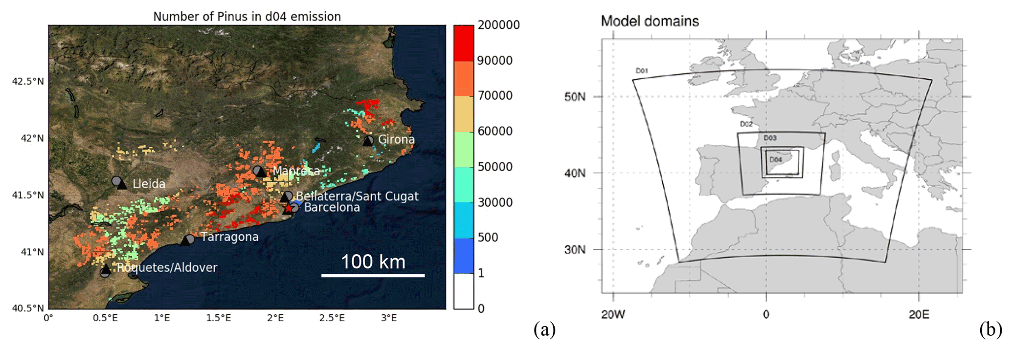
Figure 1 (a) Pine tree density (trees per square kilometer) in the Catalonia region at 1 km resolution. The stations of the Aerobiological Network of Catalonia (XAC) used in this work are depicted in gray circles, the meteorological stations of the Automatic Weather Stations Network of Catalonia (XEMA) in black triangles, and the lidar station is the red star. The names of the sites next to the symbols are shown in the order XAC/XEMA in cases where the stations are very close together. (b) Simulation domains are D01 at 27 km, D02 at 9 km, D03 at 3 km, and D04 at 1 km horizontal resolution. Base map source: Esri (2020).

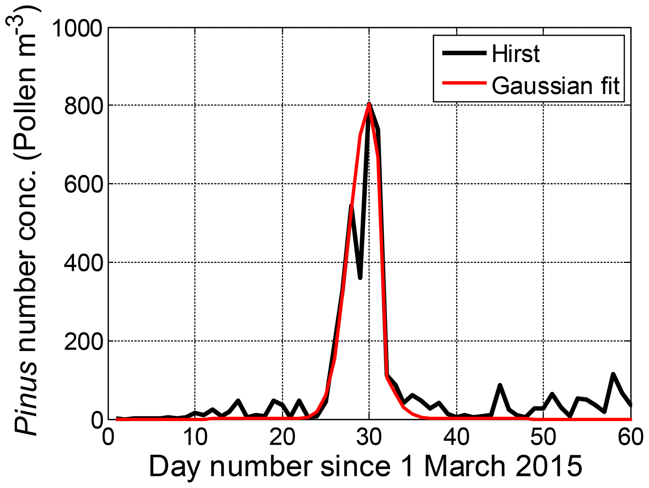
Figure 2 Pinus pollen daily concentration measured with a Hirst collector at the Barcelona site (black line) during March and April 2015 and fitted with a Gaussian curve (red line) used as phenology function, F(t), in the emission scheme of the model.

The weather-dependent function R implemented in the model accounts for the mobilization effect of the wind and turbulence of the near-surface layer of the atmosphere as follows (Helbig et al., 2004):

$$\begin{array}{}\text{(6)}& R\left(x,t\right)=K_e\cdot u_{\ast },\end{array}$$

where K_e is a wind effect scale factor between 0 and 1 (unitless), and u_∗ is the friction velocity (m s⁻¹). K_e is parameterized using a threshold friction velocity, $u_{{\ast }_{te}}$, as follows:

$$\begin{array}{}\text{(7)}& {\displaystyle }{K}_e=\left\{\begin{array}{l}\mathrm{1}-\frac{u_{{\ast }_{te}}}{u_{\ast }},u_{\ast }>u_{{\ast }_{te}}\\ \mathrm{0},u_{\ast }\le u_{{\ast }_{te}}\end{array}\right.\text{(8)}& {\displaystyle }{u}_{{\ast }_{te}}=\mathit{\alpha }\cdot u_{{\ast }_t}.\end{array}$$

The threshold friction velocity is the product of a resistance term, α, and a standard threshold friction velocity, $u_{{\ast }_t}$ (m s⁻¹). The expression of $u_{{\ast }_t}$ is the regression formula of Greeley and Iversen (1985), based on wind tunnel data for sand erosion. The resistance term α is used to distinguish the different natures of sand erosion on the ground and the pollen release above the canopy height, and it is defined as follows:

$$\begin{array}{}\text{(9)}& \mathit{\alpha }={\displaystyle \frac{u_{\mathrm{10}e}}{u_{\mathrm{10}}}},\end{array}$$

where u_10e is an empirical threshold wind speed for the type of tree (m s⁻¹), and u₁₀ is the 10 m wind speed of the model (m s⁻¹). No specific values of u_10e are found in the literature for pine trees; here we set u_10e to 2.9 m s⁻¹, using the value of Helbig et al. (2004) for alder. Zhang et al. (2014) did not find significant sensitivity to different values of u_10e.

3.3 Model setup and runs

To study the dispersion of Pinus pollen in the region of study, the MONARCH model has been configured with four domains, using the telescoping nest capability of the system (see Fig. 1b). A parent domain covering central Europe, and centered over the region of interest, is set with 27 km horizontal resolution and 48 vertical layers, with the top of the atmosphere at 50 hPa. A total of three nested domains are defined to increase the model resolution up to 1 km in the innermost domain, with a ratio of 1 : 3 from one nest to the other.

The simulations cover the period 20 March to 2 April 2015, which comprises the pollination event under study in this work. The meteorological initial and boundary conditions are obtained from the ERA-5 reanalysis at 30 km horizontal resolution and 6 h frequency. No boundary conditions for the Pinus pollen are prescribed in the parent domain, as the contribution from long-range transport is considered minor compared with the local emissions. The model outputs the Pinus pollen mass concentration over the domain of study with an hourly resolution that is converted to number concentration as a diagnostic tool.

Note that the Pinus pollen mask used in all domains is the one described in Sect. 3.2 and only considers the trees of the Catalonia region pollinating during March and April. The main objective of the work is to assess the vertical distribution of pollen nearby the Barcelona site where the lidar is available. We consider that the Pinus pollen detected by the lidar and collected by the Hirst instruments is mainly of local origin, as the size of the pollen is significantly coarse and limits the long-range transport of this type of bioaerosol. To explore this initial hypothesis, the following two different runs were conducted: (1) a base case simulation, using the model parameters described in Sect. 3.1, and (2) an enhanced simulation, where the lifetime of the Pinus pollen is increased by assuming that the sedimentation and dry deposition of the pollen is half of what is estimated in the base case. A global calibration factor C of 2.9 was used to minimize the error of the base case simulation with respect to the Hirst observations. Other works use C as a 2D spatial factor to calibrate the emission flux better due to the large uncertainties of most pollen emissions schemes and input data sets (e.g., Kurganskiy et al., 2020). In Sect. 5, the model results for both scenarios are discussed with the Hirst and lidar measurements.

4 Conversion of lidar- and model-derived magnitudes to number concentration

We propose performing a closure study between in situ and column measurements by constraining the lidar retrieval in the first part of the vertical profile to the concentration measurement of the Hirst collector. An important added value is that the closure study also fixes parameters needed for the conversion of the model output. In order to compare the lidar retrieval to measurements made near the ground level, we consider the first lidar measurement (225 m) to be a proxy of what it would be near the ground level. This hypothesis is somehow validated by the fact that the lidar vertical distribution, as it will be shown later, is rather flat (concentrations barely vary) as one comes closer to the ground. Let us note that the Hirst collector is situated on the roof of a building at 23 m above ground level. According to Rojo et al. (2019), the effect of height on pollen concentrations is mainly determined by differences within the first 10 m above ground. In the case of the model, we consider the first model layer, the center of which varies between 24 and 24.4 m over all the simulations considered here.

4.1 Definition of magnitudes and conversion formulas

From the analysis of the samples of the Hirst collectors, the concentration of the pollen type i, $C_{\mathit{\#},i}^{\mathrm{H}}$ (pollen per cubic meter; hereafter Pollen m⁻³), is obtained. The manual procedure to do so includes neither annotating information on the size of the pollen grain, nor any kind of information on its optical properties. This observation is taken as the reference value against which the lidar retrieval is constrained and to which the model output is compared.

The lidar instrument measures the particle backscatter coefficient from which the total pollen contribution, i.e., the total pollen backscatter coefficient, β_pol (meters per steradian; hereafter m⁻¹ sr⁻¹), can be extracted as in Sicard et al. (2016a). The total pollen mass concentration, $C_{\mathrm{m}}^{\mathrm{lid}}$ (kg m⁻³), is obtained using the following relationship:

$$\begin{array}{}\text{(10)}& C_{\mathrm{m}}^{\mathrm{lid}}={\displaystyle \frac{{\mathit{\beta }}_{\mathrm{pol}}\mathrm{LR}}{{\mathit{\sigma }}^{\ast }}},\end{array}$$

where LR (steradian) is the lidar ratio, and σ^∗ (square meters per gram; hereafter m² g⁻¹) is the specific extinction cross section. The latter is actually not a fixed constant, as it will depend on the taxa present, their concentration, and weight, as well as their optical properties. It is thus virtually unknown.

The mass concentration of Eq. (10) can be converted into number concentration of the pollen grain i, $C_{\mathit{\#},i}^{\mathrm{lid}}$ (Pollen m⁻³), as follows:

$$\begin{array}{}\text{(11)}& C_{\mathit{\#},i}^{\mathrm{lid}}={\displaystyle \frac{C_{\mathrm{m}}^{\mathrm{lid}}\mathrm{wf}\left(i\right)}{\frac{\mathrm{4}\mathit{\pi }}{\mathrm{3}}{\left(\frac{D\left(i\right)}{\mathrm{2}}\right)}^{\mathrm{3}}\mathit{\rho }\left(i\right)}}={\displaystyle \frac{{\mathit{\beta }}_{\mathrm{pol}}\mathrm{LR}\mathrm{wf}\left(i\right)}{{\mathit{\sigma }}^{\ast }\frac{\mathrm{4}\mathit{\pi }}{\mathrm{3}}{\left(\frac{D\left(i\right)}{\mathrm{2}}\right)}^{\mathrm{3}}\mathit{\rho }\left(i\right)}},\end{array}$$

where for each pollen grain i wf(i) is the weight factor, D(i) (meters) is the diameter, and ρ(i) (kg m⁻³) is the mass density. It is important to note that, in this last conversion, the volume of a pollen grain is calculated assuming that the grain has a spherical shape, in agreement with the assumption made in the model. wf(i) represents the fraction of the mass of the pollen grain i to the total pollen mass. It is calculated on a daily basis, using the daily concentration measurements of the Hirst collectors as follows:

$$\begin{array}{}\text{(12)}& \begin{array}{rl}\mathrm{wf}\left(i\right)& ={\displaystyle \frac{C_{\mathit{\#},i}^{\mathrm{H}}\frac{\mathrm{4}\mathit{\pi }}{\mathrm{3}}{\left(\frac{D\left(i\right)}{\mathrm{2}}\right)}^{\mathrm{3}}\mathit{\rho }\left(i\right)}{{\sum }_u\left[C_{\mathit{\#},u}^{\mathrm{H}}\frac{\mathrm{4}\mathit{\pi }}{\mathrm{3}}{\left(\frac{D\left(u\right)}{\mathrm{2}}\right)}^{\mathrm{3}}\mathit{\rho }\left(u\right)\right]}}\\ & ={\displaystyle \frac{C_{\mathit{\#},i}^{\mathrm{H}}{D}^{\mathrm{3}}\left(i\right)\mathit{\rho }\left(i\right)}{{\sum }_u\left[C_{\mathit{\#},u}^{\mathrm{H}}{D}^{\mathrm{3}}\left(u\right)\mathit{\rho }\left(u\right)\right]}}.\end{array}\end{array}$$

In Eq. (11), the product $C_{\mathrm{m}}^{\mathrm{lid}}\mathrm{wf}\left(i\right)$ represents the mass concentration estimated from the lidar-measured total backscatter coefficient for the pollen grain i and is directly comparable to the model output. This implies that the choice of D(i) and ρ(i) has no impact on the comparisons of the lidar and the model.

Finally, the model provides mass concentration for the pollen grain i, $C_{\mathrm{m},i}^{\mathrm{mod}}$ (kg m⁻³). The number concentration of the pollen grain i is then calculated as follows:

$$\begin{array}{}\text{(13)}& C_{\mathit{\#},i}^{\mathrm{mod}}={\displaystyle \frac{C_{\mathrm{m},i}^{\mathrm{mod}}}{\frac{\mathrm{4}\mathit{\pi }}{\mathrm{3}}{\left(\frac{D\left(i\right)}{\mathrm{2}}\right)}^{\mathrm{3}}\mathit{\rho }\left(i\right)}}.\end{array}$$

The next step is to optimize all parameters to minimize the difference between the two observations, $C_{\mathit{\#},i}^{\mathrm{H}}$ and $C_{\mathit{\#},i}^{\mathrm{lid}}$, and then apply these optimum parameters to compute $C_{\mathit{\#},i}^{\mathrm{mod}}$ and compare it to both $C_{\mathit{\#},i}^{\mathrm{H}}$ and $C_{\mathit{\#},i}^{\mathrm{lid}}$.

4.2 Numerical values used in this work

The lidar number concentration, $C_{\mathit{\#},i}^{\mathrm{lid}}$, for the pollen grain i depends on the following four parameters, namely LR, σ^∗, D(i), and ρ(i), while the model number concentration for the pollen grain i depends only on two parameters, namely D(i) and ρ(i). The conversion of the lidar retrieval into number concentration has 3 degrees of freedom, while the conversion of the model output has only 1.

Each day, for the 24 h (t=1, 2, 3, …, 24) between 00:00 and 23:00 UTC, we use the least squares method to obtain the optimal specific extinction cross section by minimizing the sum of squared residuals expressed by the following:

$$\begin{array}{}\text{(14)}& \begin{array}{rl}& {\sum }_t{\left[C_{\mathit{\#},i}^{\mathrm{H}}\left(t\right)-C_{\mathit{\#},i}^{\mathrm{lid}}\left(t\right)\right]}^{\mathrm{2}}=\\ & {\sum }_t{\left[C_{\mathit{\#},i}^{\mathrm{H}}\left(t\right)-{\displaystyle \frac{{\mathit{\beta }}_{\mathrm{pol}}\left(t\right)\mathrm{LR}\mathrm{wf}\left(i\right)}{{\mathit{\sigma }}^{\ast }\frac{\mathrm{4}\mathit{\pi }}{\mathrm{3}}{\left(\frac{D\left(i\right)}{\mathrm{2}}\right)}^{\mathrm{3}}\mathit{\rho }\left(i\right)}}\right]}^{\mathrm{2}}.\end{array}\end{array}$$

This minimization can be done in terms of LR, σ^∗, D(i), or ρ(i). As the greatest unknown is without any doubt σ^∗, all other parameters (LR, D(i), and ρ(i)) are fixed. However, we also perform a sensitivity analysis on these parameters to quantify the range of uncertainty associated to σ^∗ (see Sect. 4.3). The minimization of Eq. (14) yields the best estimate solution, in terms of σ^∗, as follows:

$$\begin{array}{}\text{(15)}& {\mathit{\sigma }}^{\ast }={\displaystyle \frac{\mathrm{LR}\mathrm{wf}\left(i\right)}{\frac{\mathrm{4}\mathit{\pi }}{\mathrm{3}}{\left(\frac{D\left(i\right)}{\mathrm{2}}\right)}^{\mathrm{3}}\mathit{\rho }\left(i\right)}}{\displaystyle \frac{{\sum }_t{\left[{\mathit{\beta }}_{\mathrm{pol}}\left(t\right)\right]}^{\mathrm{2}}}{{\sum }_t\left[C_{\mathit{\#},i}^{\mathrm{H}}\left(t\right){\mathit{\beta }}_{\mathrm{pol}}\left(t\right)\right]}}.\end{array}$$

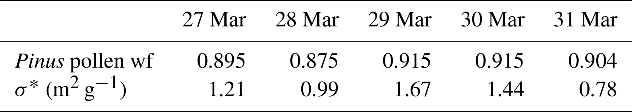
The weight factor wf(i) for Pinus pollen is calculated as the daily mean of the hourly fractions of mass concentration presented in Sicard et al. (2019). Daily values of wf(i) are reported in Table 4. The mean value over the whole event is 0.901, which is equal to saying that Pinus pollen represents 90.1 % of the mass of total pollen. The main assumption made to calculate the Pinus mass fraction is that the pollen mixture is assumed to be made only from Pinus and Platanus taxa, whereas Cladosporium and Cupressaceae were also present (Sicard et al., 2016a). However, in terms of number concentration, one sees from Sicard et al. (2019) that Pinus and Platanus represent more than 90 % of the amount of total pollen. Our assumption is equivalent to neglecting the remaining ∼ 10 %. As Cladosporium and Cupressaceae are much smaller in size than Pinus, our assumption is equivalent to neglecting, in terms of mass, probably less than 1 % of the total mass. LR is set to 50 sr, which is a reasonable value for pollen, as justified in Sicard et al. (2016a). The Pinus pollen diameter D_Pinus and mass density ρ_Pinus are taken from Jackson and Lyford (1999) and are set to 59 µm and 560 kg m⁻³, respectively, in agreement with the model (see Sect. 3.1). With these values set, we calculate σ^∗ with Eq. (15) and find the daily values reported in Table 4. Values of σ^∗ oscillate between 0.78 and 1.67 m² g⁻¹. A factor of almost 2 between the minimum and maximum values is not that surprising, taking into account the lengthy methodology followed and, in particular, the extraction of the contribution of pollen out of the total backscatter coefficient and the hypothesis made that the first lidar measurement (at 225 m) is a good proxy of what it would be at ground level. As an example, if we compare our pollen values of σ^∗ with the ones of other large particles, we find that our values are larger than mineral dust observed in southern Europe, which has values of the order of 0.5–0.6 m² g⁻¹ (Pérez et al., 2006), and they are smaller than values for sea salt surrogate estimated to be of the order of 6 m² g⁻¹ (Radney et al., 2013). These results are consistent, since pollen grains are much less dense in mass (and, thus, have a larger σ^∗) than mineral dust and because of the strong scattering properties (and, thus, large σ^∗) of sea salt.

Table 4 Summary of the daily values of wf and σ^∗.

As an illustration of how the lidar and Hirst number concentration agree with the values of σ^∗ that are found, a scatterplot of the lidar vs. Hirst concentration on 27 March (${\mathit{\sigma }}^{\ast }=\mathrm{1.21}$ m² g⁻¹) and the daily cycle of both concentrations are shown in Fig. 3. The dates of 27 March is chosen because, according to Sicard et al. (2016a), it is the day when all column properties correlate the best with the Pinus pollen surface concentration. The scatterplot is rather disperse around the 1 : 1 line (Fig. 3a); hence the correlation coefficient, equal to 0.55, is not very high. One sees that both lidar and Hirst concentration daily cycles agree relatively well (Fig. 3b), except in the very first hours of the day when no pollen is detected in the column, whereas it is present at the surface.

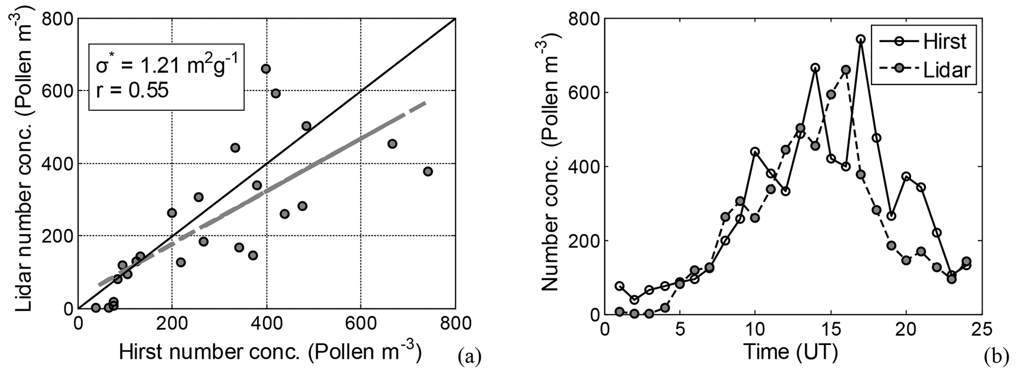
Figure 3 (a) Scatterplot of lidar vs. Hirst Pinus number concentration at or close to the ground level on 27 March, with ${\mathit{\sigma }}^{\ast }=\mathrm{1.21}$ m² g⁻¹. (b) Daily cycle of both concentrations. In panel (a), r=0.55 is the correlation coefficient.

4.3 Sensitivity study on the specific extinction cross section σ^∗

In order to quantify for the pollen type of interest in this study, Pinus, the sensitivity of σ^∗ to the rest of parameters, LR, D_Pinus, and ρ_Pinus, we vary these latter values and resolve Eq. (15). LR, D_Pinus, and ρ_Pinus are varied around their nominal value (see Sect. 4.2) as follows: 50±10 sr, 59±10 µm, and 560±200 kg m⁻³, respectively. Although the estimation of σ^∗ is made on a daily basis, it is not necessary to perform the sensitivity study for the 5 d of the event, since the relative variations in σ^∗ as a function of the same ΔLR, ΔD_Pinus, and Δρ_Pinus from 1 d to another will not be different. The sensitivity analysis is, thus, performed for 27 March, which is the day when all column properties correlate the best with the Pinus surface concentration (Sicard et al., 2016a). The dependency of σ^∗ on the rest of parameters is shown in Fig. 4. Obvious results are that σ^∗ decreases with decreasing LR and increasing D_Pinus and ρ_Pinus. The strongest sensitivity of σ^∗ is observed for D_Pinus (for LR and ρ_Pinus are equal to their nominal values; σ^∗ varies between 0.76 and 2.12 m² g⁻¹ when $D_{\mathrm{Pinus}}=\mathrm{59}\pm \mathrm{10}$ µm), while the lowest one is observed for LR (for D_Pinus and ρ_Pinus are equal to their nominal values; σ^∗ varies between 0.97 and 1.45 m² g⁻¹ when $\mathrm{LR}=\mathrm{50}\pm \mathrm{10}$ sr). In these conditions, when all parameters are fixed to their nominal values, σ^∗ will vary by $-\mathrm{0.45}/+\mathrm{0.91}$ m² g⁻¹ ($-\mathrm{37}/+\mathrm{75}$ %) around its nominal value of 1.21 m² g⁻¹ if D_Pinus differs from its nominal value by ±10 µm, it will vary by $-\mathrm{0.32}/+\mathrm{0.68}$ m² g⁻¹ ($-\mathrm{26}/+\mathrm{56}$ %) around its nominal value if ρ_Pinus differs from its nominal value by ±200 kg m⁻³, and it will vary ±0.24 m² g⁻¹ (±20 %) around its nominal value if LR differs from its nominal value by ±10 sr. In the worst-case scenario, when all parameters are relaxed, σ^∗ could vary down to 0.45 (−63 %, with regard to its nominal value) and up to 3.95 (+226 %, with regard to its nominal value). This worst-case scenario is, however, very unlikely to happen for various reasons. First, all parameters (LR, D_Pinus, and ρ_Pinus) should take their extreme values simultaneously, and this is rather improbable. Second, the probability of LR taking values of 40 (50 − 10) or 60 (50 + 10) sr is very low, as suggested by Noh et al. (2013), who found a mean columnar lidar ratio of 50 sr and a standard deviation not greater than 6 sr during a 6 d pollination event (mostly dominated by Pinus and Quercus pollen) in South Korea. Third, in terms of grain diameter, although there is a large range of Pinus grain diameter measured in different regions of the planet, i.e., 46 µm for Japanese black pine in Japan (Hirose and Osada, 2016), 51±7 µm for P. sylvestris in China (Song et al., 2012), 52 µm for P. sylvestris in the USA (Durham, 1946), 55±4 µm for P. sylvestris in Finland (Varis et al., 2011), and 51–100 µm for P. sylvestris in Austria (Halbritter, 2016), the species considered in this study (P. halepensis and P. pinea) have a narrower range of mean diameters. Roure (1985) measured the diameters of these species in the Iberian Peninsula as being 41–55, 43–65, and 47–65, respectively. The range explored in our sensitivity study, 49–69 µm, corresponds to ±10 µm around the value of 59 µm measured for P. sylvestris by Dyakowska and Zurzycki (1959) and referenced in Jackson and Lyford (1999). Fourth and last, Pinus grain density measurements are given pretty seldom in the literature. Our nominal value of 560 kg m⁻³ was taken from Jackson and Lyford (1999). Other values of 450 kg m⁻³ have been estimated for P. sylvestris in the USA (Durham, 1946) and of 550 kg m⁻³ for Japanese black pine in Japan (Hirose and Osada, 2016). The range explored in our sensitivity analysis, 360–760 kg m⁻³, is thus conservative, and extreme values of 360 and 760 kg m⁻³ are rather unlikely to be reached.

Figure 4 (a) Sensitivity study of σ^∗ to LR, D_Pinus, and ρ_Pinus performed on 27 March. The nominal set of values used in the rest of this article is indicated with a black circle.

5 Results

5.1 General overview and horizontal representativeness of the model

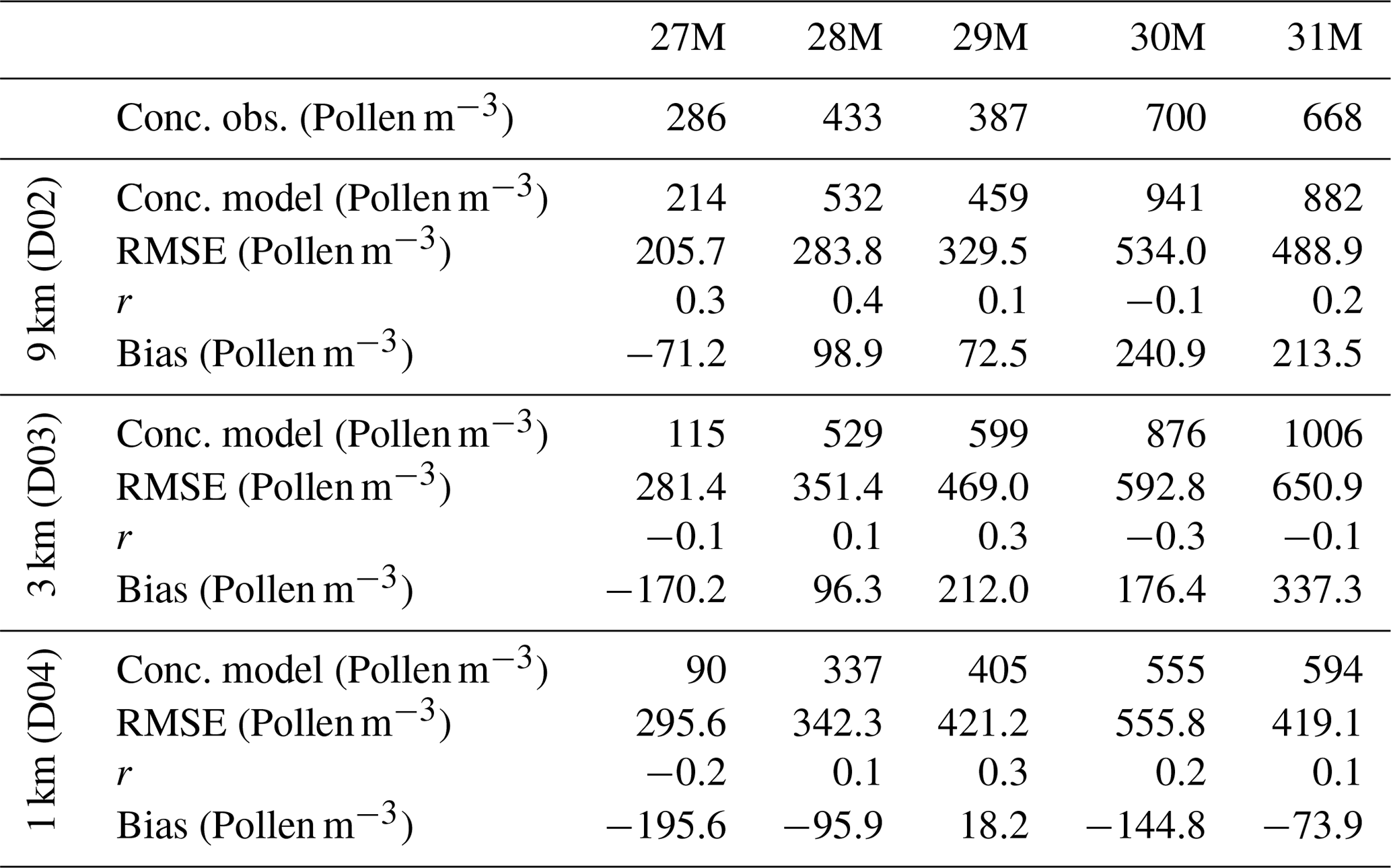
The event of interest took place between 27 and 31 March 2015, the most intense period of the Pinus pollination season in the region (Sicard et al., 2016a). The 5 d of the event are denoted as the following: 27M, 28M, 29M, 30M, and 31M. A detailed analysis of the event is presented in Sicard et al. (2016a). In the second half of March 2015, a strong anticyclone positioned in the Atlantic Ocean west of the Portuguese coast generated northwesterly winds in the northeastern part of the Iberian Peninsula. The event was characterized by medium–strong winds in the medium troposphere (500 hPa) veering from north to northwest during the 5 d of the period and resulting in northwesterly winds near the surface and clear skies in Barcelona most of the time. Figure 5a shows the hourly number concentration of the total pollen and Pinus pollen measured in the Barcelona downtown with the Hirst instrument during the event. Total pollen hourly concentrations reached values higher than 6000 Pollen m⁻³ on 31M. On every day, the Pinus pollen shows a diurnal cycle with several concentration peaks of major intensity. Figure 5b represents the fraction of the mass concentration of Pinus pollen, calculated according to Sicard et al. (2019). Pinus pollen represents 90 % of the mass of total pollen. As Pinus pollen grains are much larger than the rest of the pollen types present during this event, their contribution in mass dominates. In this work, we focus the analysis on the Pinus pollen because it is the taxon with the major contribution to the total mass of pollen measured in Barcelona, and the emission source is widely distributed across the domain of interest (see Fig. 1a). The latter allows a better analysis of the role of short-to-medium range transport and vertical mixing processes in the dispersion of this type of pollen.

Figure 5c also shows the quicklook plot, also called time–height plot, of the volume depolarization ratio of the lidar. It is not a quantitative plot, since both the molecules and the particles contribute to the volume depolarization, but it is an indicator of the presence (or not) of depolarizing particles (here, pollen grains). In Fig. 5c, the dark green areas represent the molecular level (only detectable at the high temporal resolution of the quicklook during nighttime because of the reduced background signal – as opposed to daytime), light green areas represent low-depolarizing particles (urban background), and yellow/orange areas represent high-depolarizing particles, i.e., pollen. The vertical distribution of the airborne pollen also shows a clear diurnal cycle, with usually no or weak nighttime activity in the upper layers, where the pollen grains are probably staying very close to the ground. The diurnal cycle is marked by an increase in the amplitude and height of the volume depolarization ratio, starting around 10:00 UTC, and a decrease, starting before 16:00 UTC. This diurnal pattern is observed on each single day of the pollination event. On the first 4 d, the volume depolarization ratio has come back to its background value (<0.08) before 20:00 UTC. Most of the aerosol load is usually found below 1.5 km. While the peak of Pinus pollen hourly concentration at the surface (1266 Pollen m⁻³) is reached on 30M at 08:00–09:00 UTC, the peak in the column (quantified by the pollen aerosol optical depth (AOD) in Sicard et al., 2016a) is reached 4 h later at 12:00–13:00 UTC. Note that, even though weak or no nighttime activity is detected by the lidar, the ground measurements indicate that periods with significant nighttime pollen concentrations (e.g., the first hours of 28M and 31M) are present. This is a good indication of the stratification of the pollen in the lowermost layers during the nighttime.

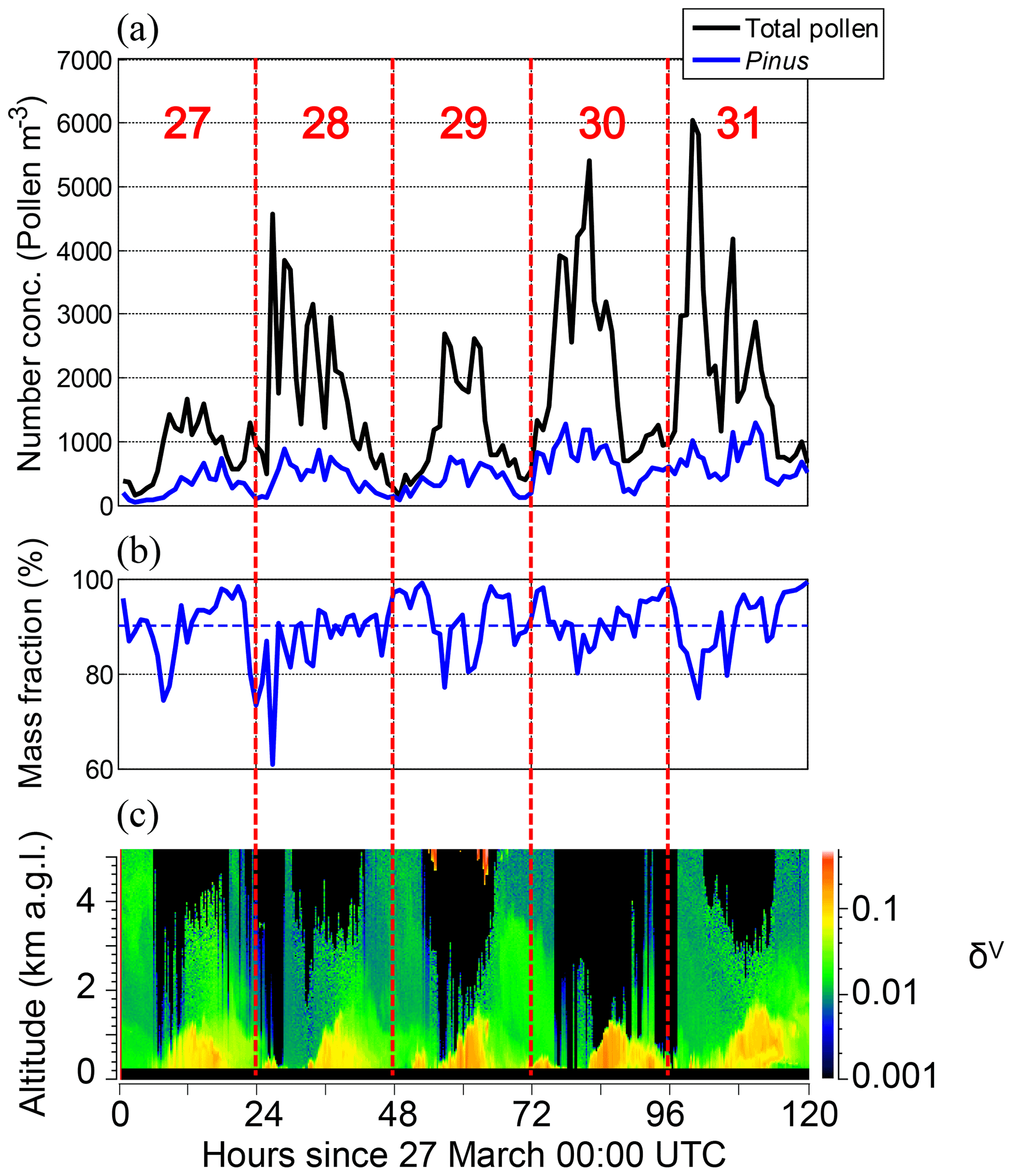
Figure 5 (a) Total pollen and Pinus number concentration. (b) Fraction of mass concentration of Pinus pollen. (c) Vertical distribution of the lidar volume depolarization ratio, δ^V, as a function of time. The period goes from 27M at 00:00 to 31M at 23:59 UTC.

In order to understand the dynamics of Pinus pollen transport during the event, we present here the model results over the innermost domain (D04) at 1 km horizontal resolution of the base case configuration described in Sect. 3. The Pinus number concentration at the surface (first model layer, around 24 m a.g.l. – above ground level), from 27M to 31M, is shown in Fig. 6. The entire event is characterized by a dispersion of pollen grains towards the Mediterranean Sea, mainly driven by the northwesterly winds. The highest concentrations are in the southwestern region of the domain. This area is dominated by the natural channelization of the Ebro valley, and a characteristic northwesterly wind, called cierzo, develops under west–northwest advection situations. Regular outbreaks of plumes with high concentrations of pollen are transported hundreds of kilometers to the Mediterranean Sea. This effect is less pronounced towards the north of the domain. Note that the regions with pines are found within the first 150 km inland from the coast (see Fig. 1a); beyond that distance, Pinus trees are scarce. The following three main areas have been identified from the pine tree density map used in the model: (1) in the south, a wide area with medium–high pine density, (2) in the central coast, the area with pines is even more extensive, with high densities of trees, and (3) in the northern coast, the presence of pines is more reduced, but there are still some localized regions with high densities of trees present. This tree distribution and the strong winds in the southwest of the domain explain the spatial gradient in concentrations simulated by the model.

Figure 6 Maps of the surface Pinus number concentration (Pollen m⁻³) simulated at 1 km resolution (D04) at 00:00 and 12:00 UTC, for the period 27M to 31M, in the green color scale. The solid line (in each plot) shows the coastline. The red circles indicate the location of Barcelona. Red dashed lines indicate the vertical cross sections shown in Fig. 10. Base map source: Esri (2020).

To assess the representativeness of the model results, we have compared them with the hourly meteorological and daily aerobiological observations described in Sect. 2. Here, we focus on surface observations. The quality of the results is quantified by means of classical statistics (Pearson correlation coefficient, r, root mean square error, RMSE, and bias), using seven aerobiological stations of the XAC network and seven meteorological stations of the XEMA network (details on the localization are in Fig. 1a and Table 1). The variables evaluated are hourly 2 m air temperature, 10 m wind speed and direction, irradiance, 2 m relative humidity, and daily Pinus number concentration at the first model layer.

Regarding the meteorological results, Table 5 presents the statistics for the 9 km base case run and all seven stations (results for 3 and 1 km in the Tables S1 and S2 in the Supplement), and Fig. 7 shows the temporal evolution of the same variables (except concentration) at the three model resolutions for Barcelona and Bellaterra/Sant Cugat (results at the other five stations in Fig. S1 in the Supplement). The statistics indicate a good agreement for the temperature, irradiance, and relative humidity in most of the stations (correlations above 0.9 and low bias), while higher errors are observed in the wind. Overall, the results are within the typical performance range of mesoscale models in the area of study (i.e., Jiménez-Guerrero et al., 2008), with surface winds being one of the most difficult variables to reproduce in coastal regions with a complex terrain like the one under study. On the one hand, the model results in coastal sites may show higher errors in temperature, winds, and relative humidity. These sites are close to the sea–land interface, and small inaccuracies in the representation of the coastline may have a strong impact in the results. The Tarragona site is a clear example where the temperature results are degraded with the 1 km domain compared with the upper nests (see the Supplement) as a result of the land and sea grid cells represented in each model resolution surrounding the site. An excessive influence of marine air masses will result in a lower thermal amplitude and overestimated relative humidity. On the other hand, better statistics are obtained at inland sites where the topography is properly captured by the model resolution. Most sites show RMSE and bias below 2.6 and ±1.2 ^∘C, 2 and ±0.5 m s⁻¹, 90 and ±11^∘, and 15 % and ±6 % for temperature, wind speed, wind direction, and relative humidity, respectively.

The Barcelona site is representative of a coastal station, located few kilometers off the shore, while Bellaterra/Sant Cugat is an example of an inland site not affected by major mountain ranges (i.e., the Pyrenees). At both stations an improvement is detected in most meteorological variables with the increase in resolution (see Fig. 7). The model reproduces the daily cycle of the temperature and relative humidity and captures the cloudiness observed during 29M and 30M. As noted in the statistics, more disagreement is seen in the wind speed, and the different resolutions show larger variability compared with the other variables. The wind results in the Barcelona site are consistent among the model resolutions. Some systematic bias is observed in the wind speed at the end of the day and during the first hours of the following day. The model overestimates the calm winds observed during nighttime, and it tends to underestimate the morning peak (i.e., transitions from 27M to 28M, 29M to 30M, and 30M to 31M). This results in lower relative humidity and higher temperatures during the calm periods compared with observations, although this does not impact the wind direction that is well captured most of the time. The results at the Bellaterra/Sant Cugat site show a clear improvement with the resolution. The site is located in a long valley surrounded by two mountain ranges that are better represented in the model by increasing the resolution. The overestimated wind during nighttime in Bellaterra/Sant Cugat results in the model wind veering from southwest to northwest (i.e., 27M and 29M), while observations show a calm, stagnated situation. Such an error leads to a model underestimation of the relative humidity and an overestimation of the temperature there. On the night of 31M, the observations show weak easterly winds, while the model develops northwesterly winds. Albeit that the limitations identified, the model captures the meteorology of the event under study reasonably well.

The main driver of the pollen release in the atmosphere is the wind. The period of study is not characterized by intense surface winds. This means that wind speed peaks are below 10 m s⁻¹ (see Figs. 7 and S1). During periods of moderate wind (around 5 m s⁻¹), the release of pollen is significantly stronger, concentrations of 300–1500 Pollen m⁻³ are simulated 200 km downwind the emission sources (see Fig. 6), and concentrations over the Mediterranean Sea above 5000 Pollen m⁻³ are not unusual (e.g., 29M at 12:00 UTC). Under weak or calm conditions (wind speed below 1 m s⁻¹), very small concentrations are simulated downwind of the sources (<100 Pollen m⁻³), while localized high concentrations are still present close to the regions with higher pine density. The strength of the wind decreases during nighttime, which reduces the dispersion of pollen and could stop the emission process. This might be explained by the presence of weak but non-negligible winds that promote some emission, an important reduction in the dispersion, and an accumulation of grains in the lower boundary layer due to a stable atmosphere.

The daily average of the Pinus surface concentration is evaluated in the XAC sites. Table 5 presents the statistics for the period 25 March to 2 April 2015 (all stations; 9 km domain), and Fig. 8 shows the temporal evolution for the same period for the Barcelona, Tarragona, and Bellaterra sites (all three domains). The model performance is significantly different at those three sites compared with the rest of the locations. The three sites are characterized by an important upwind tree density (see Figs. 1a and 6). On the one hand, the correlation is 0.5 in Barcelona, 0.6 in Tarragona, and 0.9 in Bellaterra, with a negative bias that is more pronounced in Bellaterra (−366 Pollen m⁻³). At this site, measurements show very high concentrations, particularly on 30M, that the model does not capture in intensity, although it reproduces the evolution of the event. In fact the evolution of the event is captured in the three sites; the concentration increases from 25M to 28M and reaches a maximum on 30M in Barcelona and Bellaterra and 31M in Tarragona, which is followed by a sudden decrease on 1 and 2 April when the pollination event vanishes. On the other hand, the model does not capture the measurements in the other XAC sites (Girona, Lleida, Manresa, and Roquetes; not shown). In some cases, the pine trees did not pollinate during the event but 2 weeks later (e.g., Manresa) or the week before (e.g., Roquetes; see https://aerobiologia.cat/pia/en/); in other places, the distribution of trees imposed in the model (Fig. 1a) might not be accurate enough (e.g., Girona). Even in a relatively small geographical region, the behavior of the pine trees is significantly heterogeneous due to the types of trees present, different micro-climates, and meteorological conditions. It is clear that more efforts are needed to develop accurate phenology functions and detailed maps to improve our current results, but the performances of the model over the Barcelona site are good enough to study the vertical structure of pollen there.

Table 5 Statistics (Pearson correlation coefficient r, root mean square error (RMSE), and bias) of the model surface pollen concentration daily mean and meteorology hourly mean for 9 km domain (D02) vs. measurements calculated over the period 25 March to 2 April of the event. The measurement sites are detailed in Table 1.

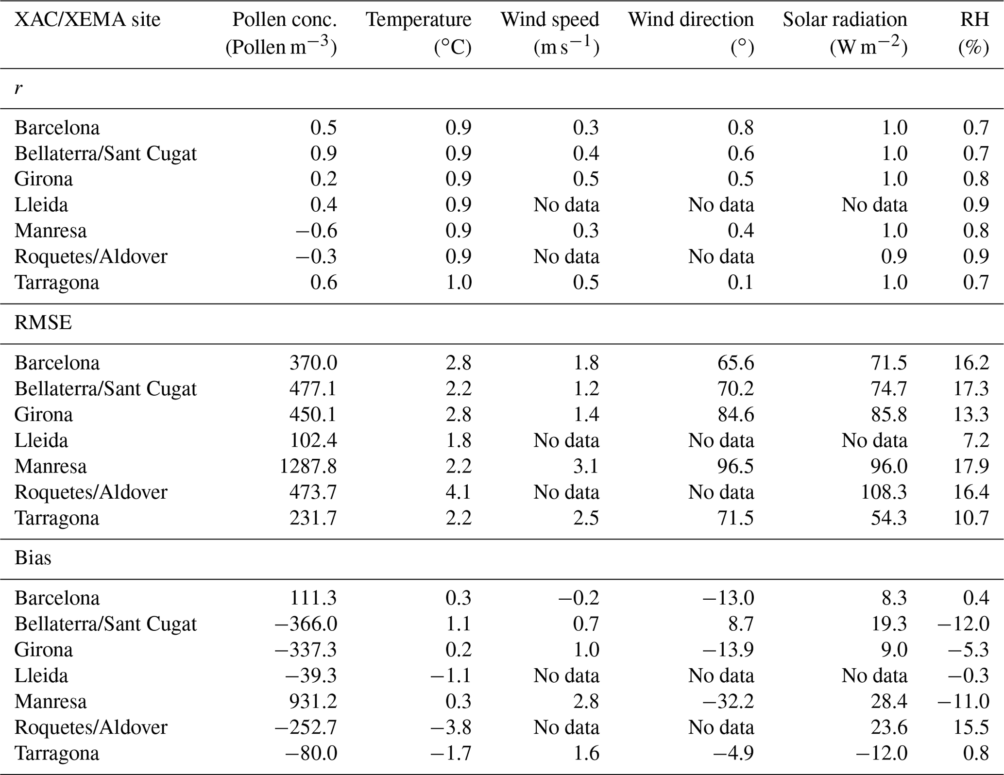
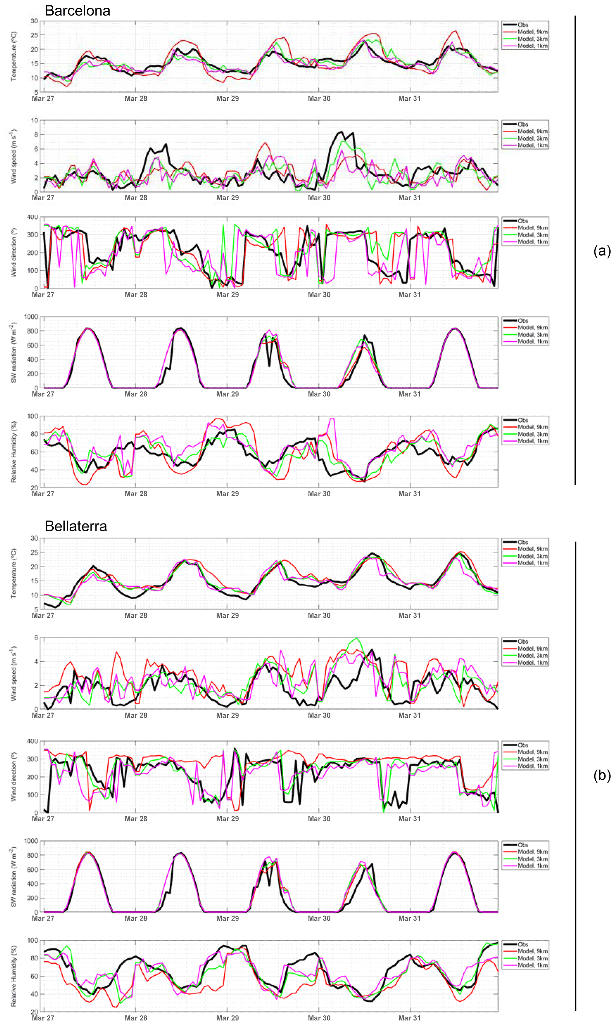
Figure 7 Comparison of the model and observations at the (a) Barcelona and (b) Bellaterra/Sant Cugat XEMA sites of 2 m air temperature, 10 m wind speed and direction, incoming shortwave radiation at surface, and 2 m relative humidity during the 5 d of the event. Colored lines represent model results at 9, 3, and 1 km resolution.

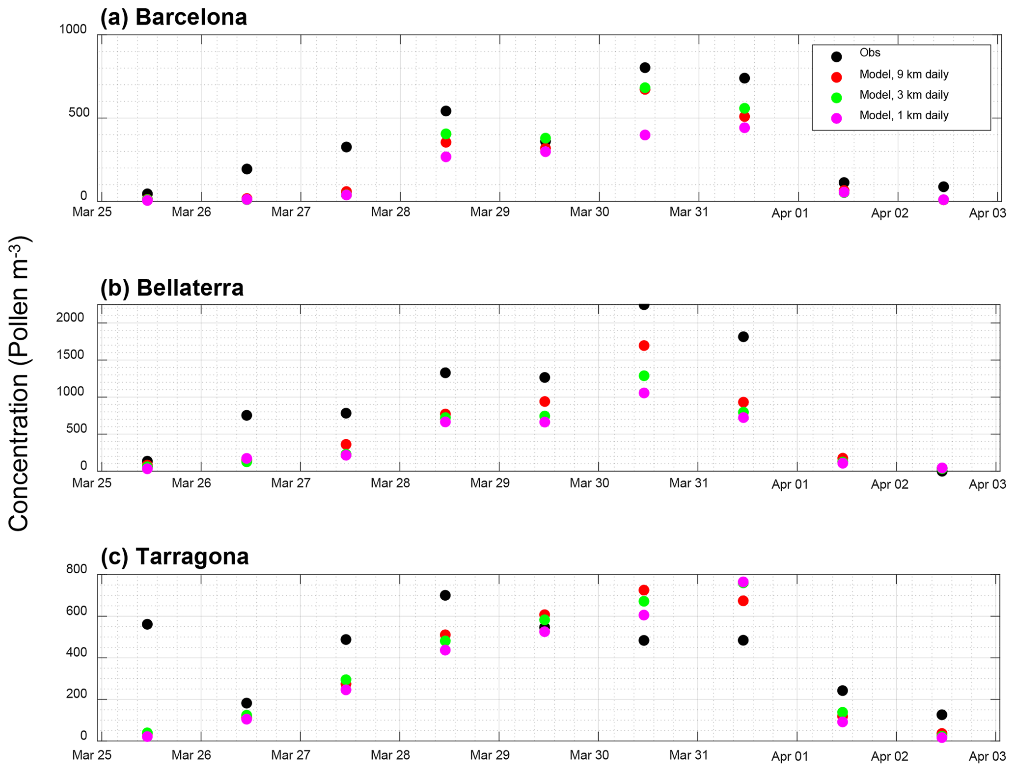
Figure 8 Daily average Pinus surface number concentration at (a) Barcelona, (b) Bellaterra, and (c) Tarragona XAC sites for the period 25 March to 2 April 2015. Colored dots represent model results at 9, 3, and 1 km resolution.

5.2 Surface concentration in Barcelona: observations and modeling

In this section, we discuss the hourly resolution results of the surface concentration at the Barcelona XAC site where specific high-temporal resolution measurements were available for the period 27M to 31M. Figure 9 shows the time series of the hourly Pinus surface concentration of the model at 9, 3, and 1 km resolution (colored lines) and the observations (black line) for the Barcelona site. Complementarily, we plot the daily averages that extend beyond the period where high-temporal resolution measurements are available. As discussed in the previous section, the model has a delay in the increase in the pollen concentration observed from 25M to 27M. During that period, although the model emits pollen grains (see Fig. 6), the concentrations in the air are strongly underestimated. The model starts to reproduce the observations on the morning of 28M, and the agreement with the observations is maintained for the rest of the event. The three model resolutions follow the trend of the measurements reasonably well. The 1 km run tends to simulate sudden rises and falls in the concentrations compared with the 9 and 3 km, which are able to maintain some background concentrations in the air. According to Fig. 9, the model is capable to reproduce the temporal variability in the observations with sudden peaks on 30M and 31M or sustained high concentrations at midday on 28M or the afternoon of 31M. Some model underestimations can be explained by the biases in the winds. For example, the strong underestimation during the first hours of 28M is attributed to the underestimated wind peak observed in Fig. 7a, or the underestimation during 29M in the morning is associated with a wrong wind direction (northerly wind in the model versus easterly wind in the observations). In this sense, the 1 km simulation is more sensitive to the errors in the wind than the upper domains. Note the need for some wind intensity in the model to capture the concentrations; under weak conditions, the model simulates extremely low concentrations pointing to the need for a minimum mobilization term in the emission scheme as suggested by other studies (e.g., Sofiev et al., 2013).

To compare the performances of the model at different horizontal resolutions, Table 6 presents the day-by-day statistics for the hourly Pinus number concentration at the Barcelona site. None of the domain resolutions is doing significantly better than the others, although, overall, the domain with the best statistical indicators (lowest RMSE and bias and highest r) is the 9 km domain. The start of the event is better captured by the 9 km domain, but the 1 km results improve significantly afterwards, resulting in lower biases. The correlations are low in most cases (around 0.2–0.3), highlighting the complexity in reproducing the hourly variability in pollen models.

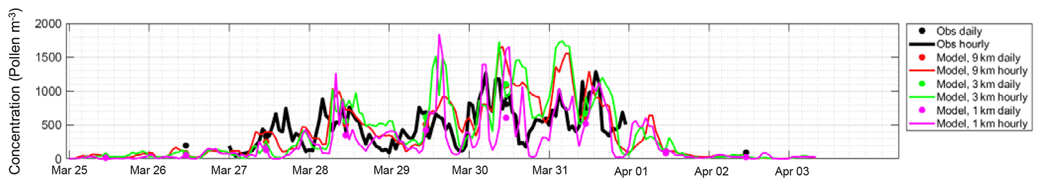
Figure 9 Comparison of the model forecast and the observations of Pinus surface number concentration during the 5 d of the event for the Barcelona site.

Table 6 Day-by-day statistics (root mean square error (RMSE), Pearson correlation coefficient, r, and bias) of the hourly model (base case) Pinus surface number concentration and measurements calculated over the 5 d of the event at the Barcelona site.

5.3 Concentration in the column in Barcelona: observations and modeling

The study of the mechanisms responsible for the pollen transport and the analysis of the model performances for predicting the vertical distribution of Pinus grains are performed in terms of two vertically integrated statistical indicators, namely the fractional bias (FB), and the Pearson correlation coefficient (r). FB and r are both calculated for the number concentration. For each vertical 1 h profile, the vertical extension considered starts at the lowest pair of simultaneously available model and observed values (fixed at 225 m, which is the height of the first valid lidar measurement) and ends at the pollen top height, h_pol, taken from Sicard et al. (2016a). Both the base case (100 % deposition; 100 % sedimentation) and the enhanced (50 % deposition; 50 % sedimentation) simulations are considered, both at the three domain resolutions of 9, 3, and 1 km. We recall that the model has been calibrated with the surface measurements (see Sect. 3.3), and thus, that the model vertical resolution of Pinus is independent from the column (lidar) measurements.

Before analyzing the results, we present the latitudinal and longitudinal cross sections of the model Pinus number concentration at the coordinates of the Barcelona lidar site (2.112^∘ E, 41.389^∘ N; see the red dashed lines in Fig. 6) for the 1 km resolution on 30M at 12:00 UTC (Fig. 10). A more vertical structure is observed in the longitudinal cross section compared to the latitudinal one where the orography is more pronounced (Pyrenees). In agreement with the emission scheme, most of the pollen dispersion occurs downwind of the second mountain range from the shore (latitudinal cross section). Above the lidar site, the model predicts a thick Pinus pollen layer up to ∼ 0.8 km and then a decrease up to ∼ 1.3 km. As it will be shown later, the model vertical structure is not always in agreement with the measurement and presents more variability with increased horizontal resolution, particularly from noon onwards.

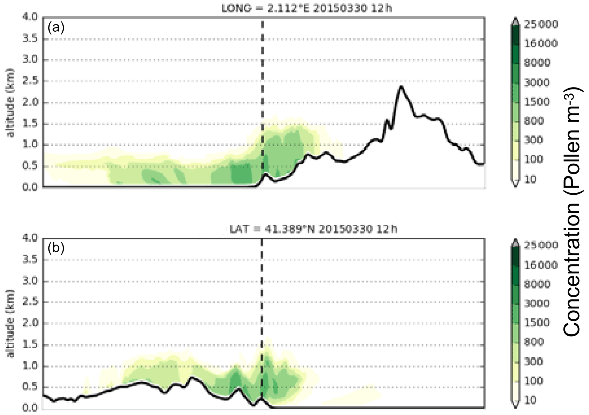
Figure 10 Vertical cross section of the Pinus number concentration (Pollen m⁻³) simulated at 1 km resolution (D04) at 12:00 UTC on 30M. The horizontal latitudinal (a) and longitudinal (b) cross sections are reported with red dashed lines in the corresponding map in Fig. 6.

In order to avoid misleading results caused by the averaging of low (nighttime) and high (daytime) concentration profiles, a first analysis is made with the diurnal (defined as the average of the hourly values between 09:00 and 17:00 UTC) statistical indicators. In Table 7, we report the diurnal average of FB and r for all 5 d of the event for both simulations at all three domain resolutions (9, 3, and 1 km). In order to investigate the variability in the model at each resolution, we also include the standard deviation ratio (SDR) defined as the ratio of the model standard deviation to the lidar standard deviation measured at the profile and averaged over the diurnal hours (09:00–17:00 UTC). Figure 11 shows that, for each of the 5 d of the event, the results of the base case simulation at 9 km resolution (the resolution resulting in the lowest statistical error at the surface; see Sect. 5.2) have daily mean (defined as the average of the hourly profiles between 00:00 and 23:00 UTC) vertical profiles of the Pinus number concentration, simulated by the model and measured by the lidar (top panels), a temporal evolution of the hourly FB and r (middle panels), and the plot of hourly FB vs. r (bottom panels). According to Table 7, the model significantly underestimates the Pinus number concentration in the column during the diurnal hours on the first (27M; $\mathrm{FB}<-\mathrm{60}$ %) and last (31M; $\mathrm{FB}<-\mathrm{27}$ %) day of the event, which is a result similar to what is found at the surface (Sect. 5.2). This is partly due to the definition of the phenology function which is fitted to the surface concentration regardless of the vertical distribution. While the Pinus daily mean number concentration increases by 50 % between 27M and 28M, the pollen AOD remains constant between both days (Sicard et al., 2016a). In these conditions, our phenology function will yield an underestimation of the vertical distribution of Pinus pollen in the column on 27M, as it is observed. The same occurs on 31M. While the Pinus daily mean number concentration decreases between 30M and 31M, the pollen AOD remains constant between both days, hence, causing the underestimation of the vertical distribution of Pinus pollen in the column observed on 31M. This result suggests that the phenology function, fitted to the surface concentration, works relatively well to also reproduce the quantity of pollen transported in the column, at least during the 3 most intense days of the event. The diurnal FB is positive ($+\mathrm{11.4}<\mathrm{FB}<+\mathrm{102.3}$) on 28M, 29M, and 30M.

The diurnal correlation coefficient is higher than 0.08 in all cases (Table 7) and varies between 0.08 and 0.92. The lowest values of r are usually reached for the 1 km resolution. At 9 km resolution (the resolution chosen for Fig. 11), r varies between 0.69 and 0.91. The middle plots of Fig. 11 show that, on each day, many values of r approach 1.00 very closely, especially on 28M, 29M, and 30M. On these 3 d, the diurnal correlation coefficient is greater than 0.83 and 0.52 for the 9 and 3 km resolutions, respectively. This result suggests that the model reproduces the shape of the Pinus number concentration vertical distribution during the diurnal hours quite well, at least during the 3 most intense days of the event (r>0.52). The bottom plots of Fig. 11 summarize the score of the model well, as far as vertically integrated FB and r are concerned. There is a large variability in the hourly values of FB varying from negative (underestimation; nighttime) to positive (overestimation; daytime), and r values are close to the ideal value of 1 on 28M, 29M, and 30M.

Table 7 Diurnal (09:00–17:00 UTC) statistics (fractional bias, FB, correlation coefficient, r, and standard deviation ratio, SDR) of the modeled vertical distribution concentration vs. lidar-derived vertical distribution for the two simulations, with each one in the three domain resolutions.

A lot of variability in FB is also observed as a function of the domain resolution considered for the simulation (Table 7). In all cases, the simulations at 1 km resolution give lower diurnal FB than at 9 and 3 km resolution. Except on 29M, the ay for which the 9 and 3 km resolution yields similar FB, the 3 km resolution gives a slightly lower FB than the 9 km one. The correlation coefficient can also vary significantly from one resolution to another; a difference of up to 0.80 (enhanced simulation on 29M) is observed between the 9 (r=0.88) and 1 km (r=0.08) resolutions (Table 7). Differences between 9 and 3 km resolutions are not higher than 0.36 (enhanced simulation on 29M). On 30M, and independently of the simulation version, the correlation coefficient is remarkably constant and equal to 0.91 for the two resolutions of 9 and 3 km. In agreement with the surface results (Sect. 5.1 and 5.2), errors in the meteorology have a major impact on the dispersion of pollen at a higher model resolution. While the structure of the plumes downwind emission sources are more well defined at 1 km resolution, small errors in the wind speed or direction result in larger errors at such a high mesoscale resolution that are smoothed at coarser resolutions due to the numerical diffusion. This is a classical problem when mesoscale models approach the 1 km horizontal resolution.

The diurnal standard deviation ratio (Table 7) also illustrates the underestimation of the model during the diurnal hours on 27M and 31M (SDR < 1 in general) and the overestimation on 28M, 29M, and 30M (SDR > 1 in general). On 28M, 29M, and 30M, the variability in the model is larger for the 3 km resolution and generally smaller for the 9 km resolution. At this resolution, the diurnal SDR varies between 1.06 on 28M (variability of the model is similar to the atmospheric variability) and 2.84 on 29M (variability of the model is ∼ 3 times larger than the atmospheric variability). From the above discussion, we conclude that the 9 and 3 km resolutions are probably the most suitable to minimize bias and maximize correlation between Pinus pollen forecast and observations in the column. The 9 km resolution also presents the advantage of reducing the model variability. The 9 km resolution is chosen for plotting the hourly and daily mean variations shown in Fig. 11.

The effect of the deposition and sedimentation on the quantity of pollen grains transported vertically is studied by means of the two simulations defined in Sect. 3.3 as the base case (100 % deposition; 100 % sedimentation) and enhanced (50 % deposition; 50 % sedimentation) simulations. The results are reported diurnally in Table 7 and daily in the top plots of Fig. 11. The study on the sedimentation is motivated by the high sedimentation velocity of large Pinus grains (3–4 cm s⁻¹; Jackson and Lyford, 1999). As an example, particles of mineral dust with a diameter smaller than 10 µm have a sedimentation velocity lower than 1 cm s⁻¹ (Li and Osada, 2007). Pollen sedimentation velocity is partly controlled by the grain size, density, and shape, all of which are highly variable. Consequently, the sedimentation velocity may be one of the main factors regulating the pollen vertical dispersion. In the case of Pinus pollen, the sacci, or inflated air bladders on each side of the grain, play an additional role in such a mechanism in that they act as aids for aerial dispersal (Wodehouse, 1935; Proctor et al., 1996; Schwendemann et al., 2007). As seen in Table 7, the combined effect of deposition/sedimentation on FB is quite notable. In the cases for which the base case simulations result in an underestimation (negative diurnal FB; see Table 7), the enhanced simulations, as expected, always reduce this underestimation and, thus, improve the model score. On the contrary, when the base case gives a positive diurnal FB, the enhanced simulation increases this value and, thus, worsens the overestimation. In terms of the fractional bias, the increase in diurnal FB, when the deposition/sedimentation is set to half of its nominal value, varies between 4.7 % (31M; 1 km) and 13.3 % (28M; 3 km). On average, over the 5 d of the event, the mean increase in diurnal FB is almost the same for all three domain resolutions, where ΔFB is 9.1 %, 10.0 % and 8.4 % for 9, 3, and 1 km resolutions, respectively. The effect of the reduction in the deposition/sedimentation is also visible on the top plots of Fig. 11 in which the results of enhanced simulations are also reported. In all cases, the concentration increase due to the reduction in deposition/sedimentation is significant. As expected, larger differences are observed in the lowermost layers. The daily relative increase in concentration (vertically integrated up to 2 km height; see the top plots of Fig. 11), due to a 50 % decrease in deposition/sedimentation, is 16.1 %, 14.1 %, 16.5 %, 13.0 %, and 9.7 % on 27M, 28M, 29M, 30M, and 31M, respectively. The deposition/sedimentation has a small effect on the capability of the model to reproduce the shape of the Pinus pollen vertical distribution (Table 7) because, from the base case to enhanced simulations, the least significant figure of the correlation coefficient does not change by more than ±0.04. To conclude this analysis, reducing deposition/sedimentation has virtually no impact on the way the model reproduces the shape of the vertical distribution of the pollen number concentration, and this suggests that other processes are more relevant to explain the vertical structures observed.

To have a closer look to the performance of the model in the column with respect to time, we plot, in Figs. 12, 13, and 14, the hourly evolution of the profiles of Pinus number concentration for the base case simulation at all three domain resolutions and for the observations on 28M, 29M, and 30M, respectively. On 28M, 29M, and 30M, the 3 most intense days of the event, a bimodal diurnal cycle of the fractional bias is visible in Fig. 11 (middle plot), showing an underestimation during the nighttime and two peaks of overestimation at 06:00–10:00 and at 15:00–16:00 UTC. The morning peak is probably due to an excessive mobilization of pollen during nighttime associated to a possible lack of ventilation during the first hours of the day.

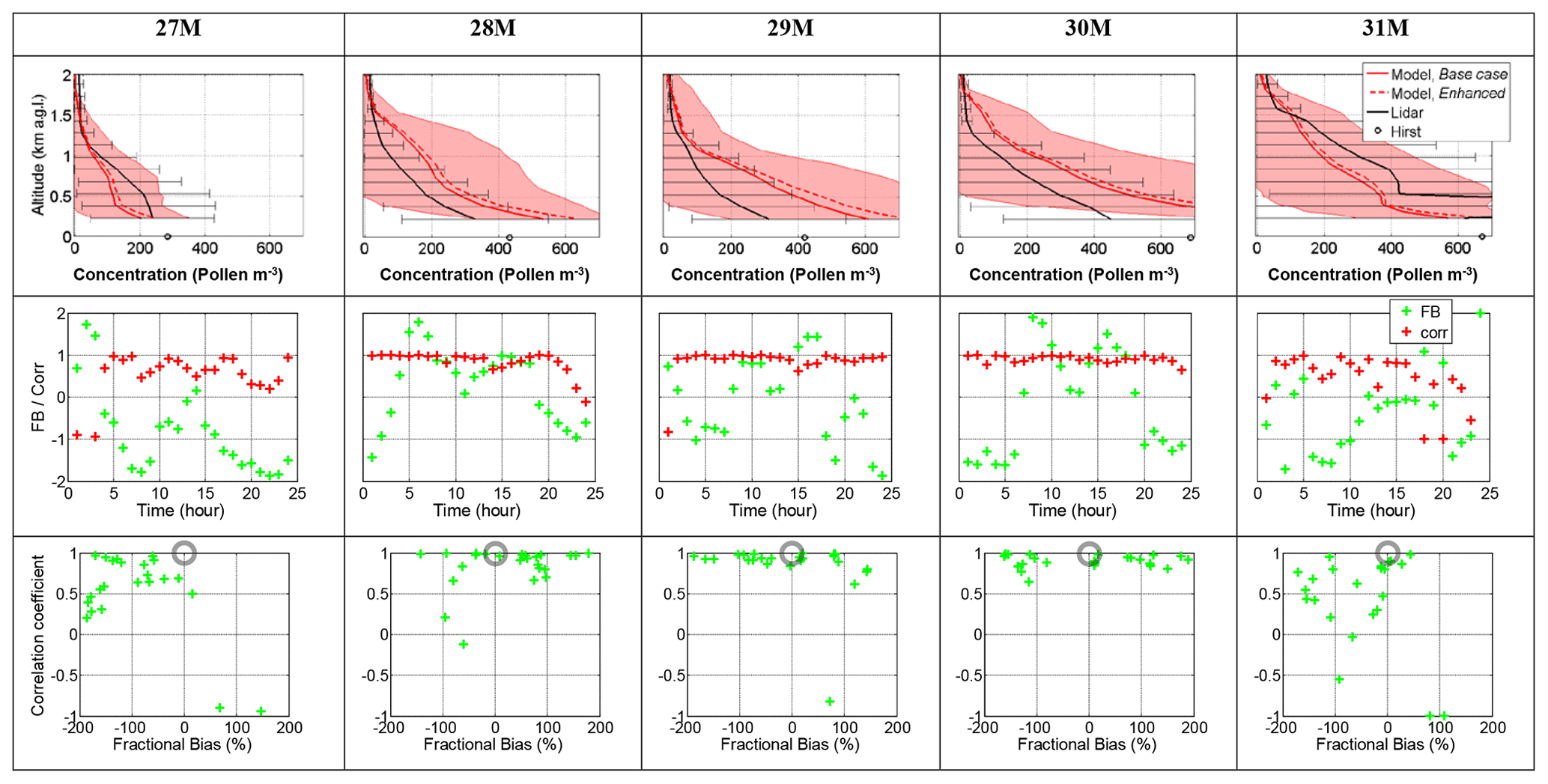
Figure 11 For each of the 5 d of the event (columns), the daily mean modeled vs. observed vertical profile (top row) of the Pinus number concentration is shown. The middle row shows the 1–24 h time evolution of the fractional bias, FB, and correlation coefficient, r, while the bottom row shows r vs. FB. In the top plots, the daily mean Hirst surface concentration is reported as a circle at the ground level for reference, and the model and lidar standard deviations are reported as shaded areas and horizontal bars, respectively. In the bottom plots, the ideal (FB, r) values (0, 1) are indicated by a gray circle. The simulation considered is the base case, with the domain resolution of 9 km (D02). In the top plots, the daily mean vertical profile of the enhanced simulation is also reported for comparison.

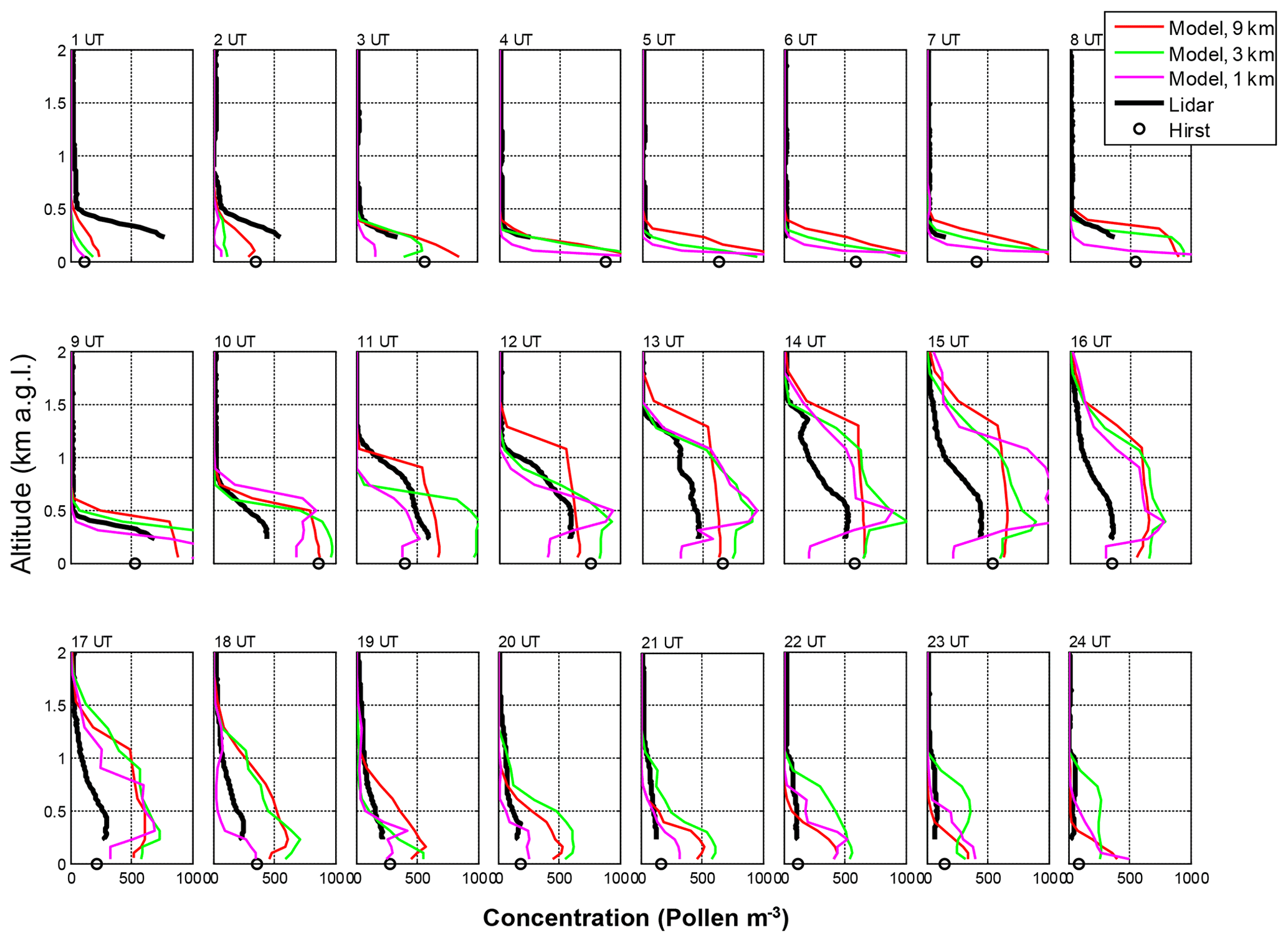
Figure 12 Hourly evolution of the vertical profile of Pinus number concentration on 28M, forecast by the base case simulation for the three domain resolutions. Hourly lidar-derived vertical profiles are reported in black. Hourly Hirst surface concentrations are reported as a black circle at ground level for reference.

Figure 13 Same as Fig. 12 for 29M.

Figure 14 Same as Fig. 12 for 30M.

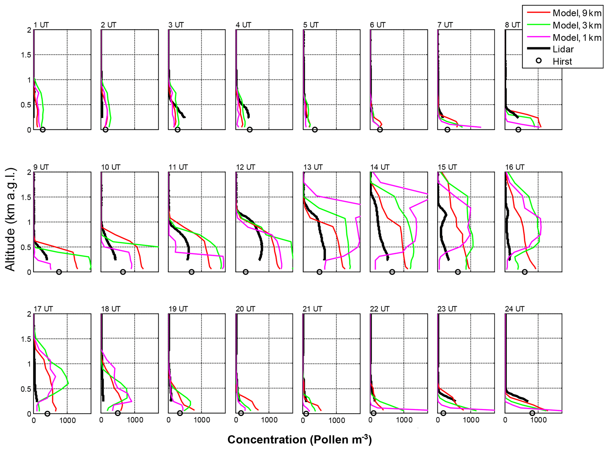
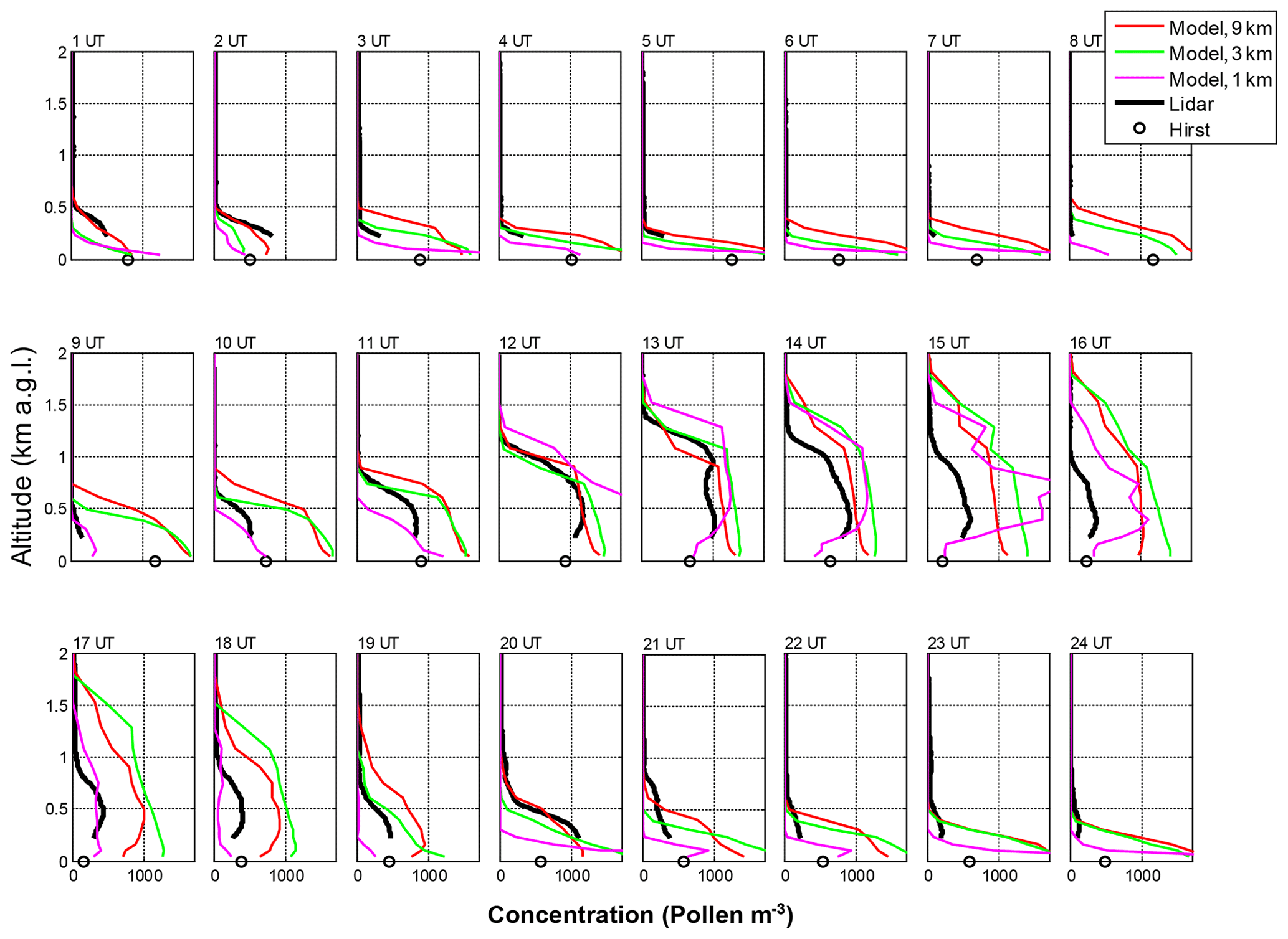
As seen in Sect. 5.1 and in Fig. 7 in particular, the model has some systematic error that induces an overestimation of nocturnal wind and underestimation of the increase in wind during the morning. The afternoon peak is likely due to the fact that pollen stays aloft longer than it does in reality, or that there is an excessive emission flux upwind during the previous hours. This behavior of the model is presented in Figs. 12, 13, and 14. According to the lidar, the pollen layer grows between 09:00–14:00 UTC, following a typical development of the convective boundary layer. During that period, the top of the layer is well reproduced by the model with excessive mobilization of pollen grains, depending on the horizontal resolution and hour. Note the good agreement in some specific profiles, see, e.g., on 30M at 12:00–13:00 UTC for 3 km (Fig. 14). The sink of the layer is observed between 14:00 and 15:00 UTC on 28M and 29M (the model predicts it 1 h later) and between 13:00 and 14:00 UTC on 30M (the model predicts it 2 h later). The delay of the model in predicting the pollen layer drop in the afternoon might be linked to the fact that the model delays the decay of the convective boundary layer. In the afternoon, and especially for the 1 km resolution, the model predicts a strong and steep decrease in concentration towards the surface. The same result is observed with the surface concentration in Sect. 5.2, where the simulation at 1 km resolution shows a decrease in concentration (which leads to an underestimation of the model; see Fig. 9), followed by sudden peaks that correlate well with the wind speed. Again, it shows the higher sensitivity to wind speed and direction of the 1 km simulation compared to the 3 and 9 km simulations. Also, more structures are visible at 1 km resolution than at the other resolutions. The finer the resolution, the more vertical structures can be seen. However, the structures visible at the 1 km resolution are not always reproducing reality (see, e.g., on 29M at 14:00 UTC; Fig. 13).

The Hirst observations are much more variable than the model concentration and the meteorology. Although following a general trend, the Hirst concentrations oscillate up and down most of the time and throughout the whole day (see the black circles in the hourly plots of Figs. 12, 13, and 14, and the black line in Fig. 9), while the model concentration usually steadily increases in the morning and decreases in the afternoon after 15:00–17:00 UTC. Such a difference between model and observations is not visible in the meteorological variables (Fig. 7). In fact, for some variables, the opposite happens, e.g., the model wind speed is more variable than the observation. The high variability in the observed Pinus concentration, independent of the meteorology, emphasizes again the difficulty in predicting airborne pollen grain concentration and the need to develop emission schemes especially designed for bioaerosols, the emission of which is much more complex than that of the rest of natural particles.

6 Conclusions

This paper combines pollen concentration surface (Hirst) and columnar (lidar) measurements, as well as an atmospheric transport model, with a simplified pollen module especially implemented for this study to improve our understanding of pollen vertical dispersion, distribution, and mixing in the atmospheric column. The pollen type under study is Pinus, and the event of interest is a 5 d pollination event which occurred in the region of Barcelona, NE Spain, during 27–31 March 2015. Prior to the analysis, conversion formulas are given to convert lidar-derived total backscatter coefficient and model-derived Pinus pollen mass concentration into a Pinus pollen number concentration, which is the magnitude measured at the surface. The most sensitive conversion is the backscatter coefficient, which is based on the specific extinction cross section, a critical parameter that is virtually unknown, so a sensitivity analysis is carried out on the latter. Its estimation is made by minimizing the sum of the squared residuals between the surface concentration, and the first lidar measurement taken as a proxy of what it would be at ground level. In the conditions of our case study, the specific extinction cross section oscillates between 0.78 and 1.67 m² g⁻¹. To our knowledge, it is the first time a relationship between the optical and mass properties of atmospheric pollen has been quantified in ambient conditions.

Nested numerical simulations at 9, 3, and 1 km horizontal resolution are deeply analyzed, in addition to the effects of sedimentation and dry deposition. The model used is the Multiscale Online Nonhydrostatic AtmospheRe CHemistry model (MONARCH) developed at BSC. Pinus pollen grains are represented as a spherical particle with hygroscopic growth factors, following Griffiths et al. (2012), which affects the density of the particle while keeping its size constant. The emission scheme is based on the concepts of the parameterization of Helbig et al. (2004). One of its most critical parts is the phenology function, which, in our work, is constrained by the observed pollen counts by fitting a Gaussian function to the evolution of the pollen concentration during the period 1 March–30 April 2015. The spatial distribution of pine trees, obtained from the cartography of habitats of Catalonia (Carreras et al., 2015) and the inventory of the Barcelona city council, has been remapped to a 1 km resolution data set and then combined with the pine tree density reported by the Forest Inventory of Catalonia (Gracia et al., 2000–2004). The representativeness of the model results is assessed by comparing them with hourly meteorological and daily aerobiological observations from several points in Catalonia. In general, the statistics indicates a good agreement for temperature, irradiance, and relative humidity at most of the stations (correlations above 0.9 and low bias), while higher errors are observed in the wind. A better statistic is observed at inland sites compared to coastal sites. The good agreement of the model meteorology with the observations in the horizontal scale is a mandatory requirement for the assumptions made to calibrate the lidar with the Hirst sampler (which are 4.4 km apart). At the Barcelona site, where the lidar is located, an improvement is detected in most meteorological variables with the increase in resolution. The model reproduces the daily cycle of the temperature and relative humidity; more disagreement is seen in the wind speed, and the different resolutions, although consistent one to another, show larger variability compared with the other variables. The model overestimates the calm winds observed during nighttime, and it tends to underestimate the morning peak. This results in lower relative humidity and higher temperatures during the calm periods compared with the observations. When combining both analyses of hourly surface and column concentration vs. model, the following results are found:

• The three model resolutions follow the evolution of the measurements in general. The 1 km run tends to simulate sudden rises and falls in the concentrations compared with the 9 and 3 km, which are able to maintain some background concentrations in the air. Although the simulation at 1 km may improve the model score in places with complex topography, the meteorological errors in the wind have larger impacts in such a high-resolution configuration. In this sense, the combination of the three resolutions provides complementary information to advance our understanding in key driving processes, but 9 or 3 km simulations might be preferred for specific forecasting applications.

• The largest discrepancies between measured surface (Hirst) and column(lidar) concentrations occur during the nighttime as no pollen is detected in the column, whereas it is present at the surface. This is likely due to the limitation of the lidar for measurements below 225 m where most of the stable boundary layer resides. Simulated profiles at different resolutions show large variability throughout the event of study. During nighttime, the model tends to overestimate the amount of pollen available in the stable boundary layer compared with the Hirst concentration, but matches its top when it is detected by the lidar. Such an overestimation may be attributed to systematic errors in the wind speed during midnight. This points out that the wind is the main driver of the nighttime/early morning pollen activity.

• A 50 % decrease of the sedimentation/deposition parameter increases the daily column concentration 10 %–17 %. Decreasing the deposition/sedimentation in the model is not enough to significantly change the results on a daily basis. Both parameters only have a limited impact on the vertical concentration, suggesting that other processes are more relevant to reproduce the measurements. These mechanisms might have a larger impact during nighttime and would deserve further investigation.

• Finally, from our model results, the vertical structure of the pollen is mainly controlled by the vertical mixing within the boundary layer and the sensitivity of the emission scheme to winds. In general terms, the model matches the depth of the pollen layer during stable conditions and the growth of the convective boundary layer, but systematic biases are detected in the second half of the day, with persistent overestimation within the convective boundary layer. During the latter period, lidar profiles do not extend up to the top of the boundary layer, probably because of gravity effects that are not well represented by the model.

The results of the study emphasize the tremendous importance of the completeness of the tree spatial distribution, density, and type. Even in a relatively small geographical region, the behavior of the pine trees is significantly heterogeneous due to the presence of different pine species, different micro-climates, and meteorological conditions. The assumption made in the model that the availability of pollen grains in the pine trees (P. halepensis; P. pinea) of the region is the same during the pollination event is far from being close to reality. A clear outcome of this study is the need for more research in the development of phenology functions for bioaerosols, which, unlike the rest of aerosols, do not respond only to physical laws. While biologically based phenology functions are not readily available, current model approaches will still be based on parametric schemes strongly relying on aerobiological measurements and refined calibration procedures. In this sense, approaches like deriving specific calibration factors per nested domain or implementing 2D spatial calibration factors (e.g., Kurganskiy et al., 2020) might improve the performances of the model even in small regions. Once more reliable emission schemes are available, the role of processes that have shown limited impact on the vertical structure of the pollen, like sedimentation/dry deposition, might be more relevant.

The proposed methodology requires a Hirst sampler nearby a polarization-sensitive lidar, first, for the confirmation of the presence and the type of pollen observed and, second, for the conversion of the lidar-derived backscatter coefficient into number concentration (through the retrieval of the specific extinction cross section). To apply the methodology at sites with no Hirst sampler, but at least knowing the most probable predominant pollen type present, a look-up table would be needed. Such a table can be obtained by applying the methodology at a site with both a polarization-sensitive lidar and a Hirst sampler on a large number of pollen loads with different predominant pollen types and over a relatively long period of time. This is a guideline for future work.