the Creative Commons Attribution 4.0 License.
the Creative Commons Attribution 4.0 License.
 | 03 Dec 2021
Long-term atmospheric emissions for the Coal Oil Point natural marine hydrocarbon seep field, offshore California
Christopher Melton
Donald R. Blake
In this study, we present a novel approach for assessing nearshore seepage atmospheric emissions through modeling of air quality station data, specifically a Gaussian plume inversion model. A total of 3 decades of air quality station meteorology and total hydrocarbon concentration, THC, data were analyzed to study emissions from the Coal Oil Point marine seep field offshore California. THC in the seep field directions was significantly elevated and Gaussian with respect to wind direction, θ. An inversion model of the seep field, θ-resolved anomaly, THC′(θ)-derived atmospheric emissions is given. The model inversion is for the far field, which was satisfied by gridding the sonar seepage and treating each grid cell as a separate Gaussian plume. This assumption was validated by offshore in situ data that showed major seep area plumes were Gaussian. Plume total carbon, TC (TC = THC + carbon dioxide, CO2, + carbon monoxide), 18 % was CO2 and 82 % was THC; 85 % of THC was CH4. These compositions were similar to the seabed composition, demonstrating efficient vertical plume transport of dissolved seep gases. Air samples also measured atmospheric alkane plume composition. The inversion model used observed winds and derived the 3-decade-average (1990–2021) field-wide atmospheric emissions of 83 400 ± 12 000 m3 THC d−1 (27 Gg THC yr−1 based on 19.6 g mol−1 for THC). Based on a 50 : 50 air-to-seawater partitioning, this implies seabed emissions of 167 000 m3 THC d−1. Based on atmospheric plume composition, C1–C6 alkane emissions were 19, 1.3, 2.5, 2.2, 1.1, and 0.15 Gg yr−1, respectively. The spatially averaged CH4 emissions over the ∼ 6.3 km2 of 25 × 25 m2 bins with sonar values above noise were 5.7 µM m−2 s−1. The approach can be extended to derive emissions from other dispersed sources such as landfills, industrial sites, or terrestrial seepage if source locations are constrained spatially.
- Article
(9265 KB) - Full-text XML
-
Supplement
(8449 KB) - BibTeX
- EndNote


1.1 Seepage and methane
On decadal timescales, the important greenhouse gas methane, CH4, affects atmospheric radiative balance far more strongly than carbon dioxide, CO2 (IPCC, 2007, Fig. 2.21), yet CH4 has large uncertainties for many sources (IPCC, 2013) and is very sensitive to hydroxyl (OH) concentration, the primary CH4 loss mechanism (Zhao et al., 2020). Since pre-industrial times, CH4 concentrations have risen by a factor of ∼ 2.5 and after stabilizing in the 1990s and early 2000s resumed rapid growth since 2007 (Nisbet et al., 2019). The significantly shorter lifetime of CH4 than CO2 argues for CH4 regulatory priority as emission reductions (and changes to the radiative balance) manifest more quickly as atmospheric concentrations decrease (Shindell et al., 2005). Further impetus for a CH4 focus is a recent estimate that 40 % of CH4 emissions reductions are feasible at no net cost for the oil and gas, O&G, industry (IEA, 2020), a major anthropogenic CH4 source (IPCC, 2014). This is particularly salient given a recent estimate that half of recent CH4 increases are from the O&G industry (Jackson et al., 2020).
For 2008–2017, global CH4 top-down emissions estimates are 576 Tg yr−1 (1 Tg = 1012 g, range 550–594 Tg yr−1), whereas bottom-up approaches find 737 Tg yr−1 (range 594–881 Tg yr−1; Saunois et al., 2020). A significant fraction of this discrepancy arises from uncertainty in OH concentration trends and spatial variability (Zhao et al., 2020). Anthropogenic sources for 2008–2017 were estimated at 336–376 Tg CH4 yr−1 based on bottom-up estimates. Natural sources include wildfires, wetlands, hydrates, and geological seepage. Bottom-up estimates for natural sources are higher than top-down estimates (Saunois et al., 2020). Geological sources (including seepage) are estimated at 63–80 Tg CH4 yr−1 of which marine seepage is estimated to contribute 20–30 Tg CH4 yr−1 (Etiope et al., 2019) or 5–10 Tg CH4 yr−1 (Saunois et al., 2020). For comparison, marine non-geological CH4 emissions are estimated at 4–10 Tg yr−1. The broad range of this estimate arises from the uncertainty in the fraction of seabed emissions that reaches the atmosphere and the uncertainty in overall seabed emissions. Further complexity in assessing geological seepage CH4 emissions arises because both seepage and O&G emissions source from the same geological reservoirs (Leifer, 2019) and thus are isotopically similar (Schwietzke et al., 2016).
Seepage is the process by which petroleum hydrocarbon gases and fluids in the lithosphere migrate to the hydrosphere and/or atmosphere from a reservoir formation, which underlies a capping layer that seals the formation, allowing hydrocarbon accumulation. Thus, seepage requires a migration pathway, typically fractures and/or fault networks, through the capping rock layer(s) (Ciotoli et al., 2020) or where the capping layer has eroded away, forming an outcropping of the reservoir formation (Abrams, 2005).
Marine seepage is widespread in every sea and ocean (Judd and Hovland, 2007) and occurs primarily (but not exclusively) in petroleum systems and mostly in convergent basins (Ciotoli et al., 2020). Quantitative seepage estimates (for global budgets) are limited (though growing); see Leifer (2019) review and below for more recent studies. Fluxes for individual marine seep vents and seep areas have been reported for the Gulf of Mexico (Römer et al., 2019; Leifer and Macdonald, 2003; Weber et al., 2014; Johansen et al., 2020, 2017), the Black Sea (Greinert et al., 2010), the southern Baltic Sea (Heyer and Berger, 2000), various sectors of the North Sea (Borges et al., 2016; Römer et al., 2017; Leifer, 2015), offshore Norway (Muyakshin and Sauter, 2010; Sauter et al., 2006), offshore Svalbard in the Norwegian Arctic (Veloso-Alarcón et al., 2019), offshore Pakistan (Römer et al., 2012), offshore the arctic Laptev Sea (Leifer et al., 2017), the East Siberian Arctic Sea (Shakhova et al., 2013), the South China Sea (Di et al., 2020), New Zealand's Hikurangi Margin (Higgs et al., 2019), the Cascadia Margin (Riedel et al., 2018), and the Coal Oil Point (COP) marine hydrocarbon seep field, hereafter COP seep field, in the northern Santa Barbara Channel, offshore southern California (Hornafius et al., 1999), and for numerous individual vents in the field (Leifer, 2010).
Most seep emission estimates are snapshot values from short-term field campaigns. Seep emissions vary on timescales from tidal (Leifer and Boles, 2005; Römer et al., 2016) to seasonal (Bradley et al., 2010) to decadal (Fischer, 1978; Leifer, 2019). Additional temporal variability arises from transient emissions – pulses lasting seconds to minutes (Greinert, 2008; Schmale et al., 2015) to decades (Leifer, 2019). This shortcoming is being addressed by benthic (seabed) observatories and cabled observatories, e.g., Wiggins et al. (2015), Greinert (2008), Römer et al. (2016), Kasaya et al. (2009), and Scherwath et al. (2019). Still, benthic observatories are costly and thus uncommon.
Seepage contributes to oceanographic budgets and to a lesser extent to atmospheric budgets due to water column losses with significant uncertainty in the partitioning. As a result, uncertainty in the atmospheric contribution is much larger than the (significant) uncertainty in seabed emissions. Seepage partitioning between the atmosphere and ocean – where microbial degradation occurs on timescales inversely related to concentration (Reeburgh et al., 1991) – depends primarily on depth (Leifer and Patro, 2002) with little to none of the deep-sea seabed seep emissions reaching the atmosphere, e.g., Römer et al. (2019). In contrast, very shallow seepage (meter scale) largely entirely reaches the atmosphere both by direct bubble-meditated transfer and diffusive transport. For intermediate depths, the ocean–atmospheric partitioning is complex and depends on depth, bubble flux, bubble size distribution, bubble interfacial conditions, and other characteristics (Leifer and Patro, 2002). The indirect diffusive flux (proximate and distal) depends on bubble dissolution depth (Leifer and Patro, 2002), vertical turbulence transport in the winter wave-mixed layer (Rehder et al., 1999), microbial oxidation losses, and exchange through the sea–air interface.
A range of approaches have been used to estimate the sea–air flux. The most common is by measuring the atmospheric and water concentrations and applying air–sea gas exchange theory for the measured wind speeds, e.g., Schmale et al. (2005) for Black Sea seepage under weak wind speeds. Sea–air exchange is a diffusive turbulence transfer process that depends on the air–sea concentration difference and the piston velocity, kT, which depends on gas physical properties, wind speed, u (Liss and Duce, 2005), wave development (Zhao et al., 2003) including wave breaking (Liss and Merlivat, 1986), and surfactant layers at low wind speeds that suppress gas exchange (Frew et al., 2004). kT increases rapidly and nonlinearly with u and has been parameterized by piecewise linear functions (Wanninkhof et al., 2009) or by a cubic function (Nightingale et al., 2000). Air–sea gas exchange theory is for (relatively) homogeneous atmospheric and oceanographic fields (concentrations, winds, and wave development) and thus is inappropriate for point-source (bubble-plume) emissions and for the near-field downcurrent plume, which tends to be heterogeneous.
Another approach uses seabed bubble size measurements or an assumed bubble size distribution to initialize a numerical bubble propagation model to predict direct bubble-mediated atmospheric fluxes (Leifer et al., 2017; Schneider Von Deimling et al., 2011; Römer et al., 2017). The dissolved portion that evades to the atmosphere could be addressed by a dispersive model coupled to an air–sea gas exchange model, though studies have not yet addressed this component.
An alternate approach is to derive atmospheric emissions by plume inversion. Leifer et al. (2006) derived emissions for a blowout from Shane Seep in the COP seep field by a plume inversion. This neglected the portion that dissolves during bubble rise and drifts downcurrent, out of the bubble plume's vicinity before sea–air gas transfer into the atmosphere. Note that dissolved gas evasion in the plume vicinity contributes to the inversion emissions estimate.
1.2 Study motivation
In this study, we present a novel approach for assessing nearshore seepage atmospheric emissions – air quality station data modeling, specifically using a Gaussian plume inversion model. This model requires that source locations are mapped, spatially stable, and lie within a fairly constrained distance range band. These conditions are met for the COP seep field, located near the West Campus Station (WCS). The COP seep field lies in the shallow coastal waters of northern Santa Barbara Channel, CA. Spatial constraint is provided by geological structures, such as faults, that constrain emission locations. The Gaussian plume model assumes a far-field source, whereas WCS is in the near field of the extensive COP seep field. To satisfy the far-field criterion, the source was gridded, and each grid cell's emissions were treated as a distinct (distant) Gaussian plume. This characterization was validated in an offshore survey of several focused COP seep field seepage areas, whose atmospheric plumes were well-modeled as Gaussian.
Thus, this study demonstrates an approach to deriving emissions from air quality station data for an area source such as a natural marine seep field. This approach could be used to derive emissions from other dispersed sources such as landfills, industrial sites, or natural terrestrial seepage where source locations are constrained spatially.
1.3 Water column marine seabed seepage fate
The partitioning of seep seabed CH4 between the atmosphere and water column depends on seabed depth and emission character – as bubbles, bubble plumes (Leifer and Patro, 2002), or dissolved CH4. Dissolved CH4 migration through the sediment is oxidized largely by near-seabed microbes (Reeburgh, 2007), termed the microbial filter, negating its contribution and leaving only bubble-mediated migration.
As seep bubbles rise, they dissolve, losing gas to the surrounding water at a rate that decreases with time. Smaller bubbles and more soluble gases dissolve faster than larger and less soluble gases, i.e., fractionation (Leifer and Patro, 2002). Additionally, larger bubbles transport their contents upwards more efficiently than smaller bubbles (Leifer et al., 2006). Sufficiently large bubbles reach the sea surface with a significant fraction of their seabed CH4 from depths of even hundreds of meters (Solomon et al., 2009). There are synergies too, with higher plume fluxes driving a stronger upwelling flow that transports plume fluids with dissolved gases upwards towards the sea surface where air–sea gas exchange drives evasion (Leifer et al., 2009). Another synergy arises from the elevated dissolved plume CH4 concentration (Leifer, 2010; Leifer et al., 2006), which slows dissolution. Also, most COP field bubbles are oil-coated (Leifer, 2010), which slows dissolution.
Moreover, gases in bubbles that dissolve in the wave-mixed layer (or reach it by the upwelling flow) then diffuse to the sea surface due to wave and wind turbulence and then evade. Note, microbial degradation removes a portion of the dissolved CH4, which therefore never reaches the air–sea interface. Thus, there are two timescales that govern the fraction that evades – the microbial degradation timescale, which increases as concentrations decrease, and the diffusion timescale, which decreases with increasing wind speed. As a result, there is a dissolved plume that drifts downcurrent, with evasion from this drifting plume creating a linear-source atmospheric plume. Note, dissolved plume concentrations slowly decrease with time (downcurrent distance) from sea–air gas exchange losses, microbial oxidation, and dispersion, leading to a decreased atmospheric plume.
1.4 Atmospheric Gaussian plumes
Strong, focused atmospheric plumes are created from the bursting of seep plume bubbles at the sea surface and from dissolved gas evasion within the bubble surfacing footprint. This evasion is enhanced by water-side turbulence from rising and bursting bubbles (Leifer et al., 2015). Atmospheric plume evolution is described by the Gaussian plume model (Hanna et al., 1982), which relates downwind concentrations to wind transport and turbulence dispersion and is the basis of the inversion calculation (see Sect. S1 in the Supplement for details).
1.5 Setting
1.5.1 The Coal Oil Point seep field
The COP seep field (Fig. 1) is one of the largest seep fields in the world, with estimated 1995–1996 seabed total hydrocarbon, THC, emissions, EB, of 1.5 × 10⁵ ± 2 × 10⁴ m3 d−1 (Hornafius et al., 1999). Hereafter emissions and concentrations are for THC unless noted. Clark et al. (2000) estimated that half of the COP seep field EB reaches the atmosphere in the near field. This is due to shallowness, bubble oiliness, high plume bubble densities, and turbulence mixing within the wave-mixed layer.
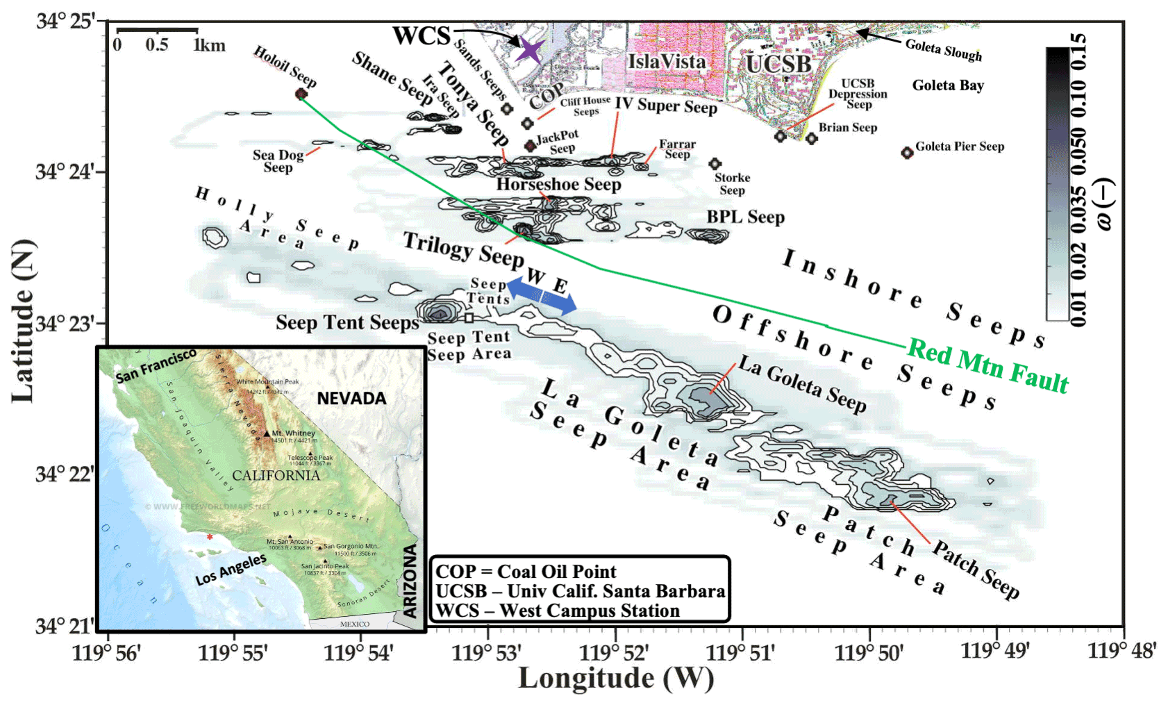
Figure 1Sonar return, ω, map after Leifer et al. (2010). Purple star marks West Campus Station. Seep area names are informal (Table S3), font size corresponds to strength. The W–E arrow segregates east and west offshore seepage. Data keys are shown in the panels. The inset shows S. California, and the red dot marks the COP seep field. California inset map from Freeworldmaps (2020).
Geological structures play a critical role in the spatial distribution of seepage (Leifer et al., 2010), which lies along several trends in waters from a few meters to ∼ 85 m deep. These trends follow geologic structures including anticlines, synclines, and faults in the reservoir formation, Monterey Formation, and overlying Sisquoc Formation. Faults and fractures associated with damage zones provide migration pathways with seepage scattered nonuniformly along the trends, including focused seep areas that are highly active, localized, and often associated with crossing faults and fractures (Leifer et al., 2010). Seepage in these areas typically surrounds a focus and decreases with distance, primarily along linear trends (Leifer et al., 2004). See Table S3 in the Supplement for informal names and locations of selected focused seep areas.
1.5.2 Coal Oil Point seep field emissions and composition
COP seep field sources from the South Ellwood oil field whose primary source rock is Monterey Formation, which is immature to marginally mature. Petroleum gases from marine organic materials have a relatively higher proportion of ethane, propane, butane, etc., relative to CH4 compared to petroleum gases from terrestrial organic materials. The wet gas fraction (C2–C5 C1–C5) indicates a thermogenic origin of greater than 0.05 (Abrams, 2017). Of the saturated alkanes, the alkenes (olefins) are of biological origin. Additionally, the ethane ethene ratio and propane propene ratio can be indicators of seep gas biogenic modification, with values above 1000 indicating purely thermogenic origin (Abrams, 2017; Bernard et al., 2001).
In this study, we analyze WCS (located at 34∘24.897′ N, 119∘52.770′ W) atmospheric THC and wind data. Clark et al. (2010) report average seep field seabed bubble gas fractions of CH4, CO2, and nonmethane hydrocarbons (NMHCs) of 76.7 %, 15.3 %, and 7.7 %, respectively, with Trilogy Seep seabed compositions of 67 %, 21 %, and 7.8 %, respectively. With respect to alkanes, seabed bubbles are 90.4 % CH4 and 8.6 % NMHC. CO2 rapidly escapes the bubbles and is negligible (< 1 %) at the sea surface. At the sea surface, CH4 in bubbles is ∼ 90 %, with NMHC making up the remaining 10 %, neglecting air gases (Clark et al., 2010). Note, whereas seep THC is predominantly CH4, THC from terrestrial directions is composed predominantly of NMHC from traffic and other anthropogenic sources as well as CH4 from pipeline leaks, terrestrial seeps, etc.
1.5.3 Northern Santa Barbara Channel climate
Diurnal and seasonal wind cycles are important to the atmospheric transport of COP seep field emissions. The Santa Barbara climate is Mediterranean with a dry season and a wet season when storms occur infrequently (Dorman and Winant, 2000). The semi-permanent eastern Pacific high-pressure system plays a dominant controlling role in weather in the Santa Barbara coastal plain. This high-pressure system drives light winds and strong temperature inversions that act as a lid that restricts convective mixing to lower altitudes. The coastal California boundary layer is shallow, from 0 to 800 m thick (Edinger, 1959), generally 240–300 m around Santa Barbara (Dorman and Winant, 2000). Additionally, coastal mountains provide physical barriers to transport (Lu et al., 1997).
As a coastal environment, the land–sea breeze is important to overall wind-flow patterns, with weak offshore night winds and stronger onshore afternoon winds (Dorman and Winant, 2000). In coastal Santa Barbara, warming on the mountaintops (and more interior arid lands) relative to the cooler marine temperatures drives the sea breeze. Downslope nocturnal flows warm nocturnal surface temperatures, moderating the coastal diurnal temperature cycle (Hughes et al., 2007).
Typical morning winds are calm, offshore, and often accompanied by a cloud-filled marine boundary layer, 50–150 m thick (Lu et al., 1997). The marine layer usually (but not always) “burns off” by mid-morning, after which temperatures rise, the boundary layer thickens, and winds shift clockwise from offshore to prevailing westerlies aligned with the coastal mountains. Midday through late afternoon and even evening, winds strengthen, often leading to whitecapping before the boundary layer collapses and winds return to the nocturnal pattern.
2.1 West Campus Station data
WCS data include wind speed, u, and direction, θ, by a vane anemometer (010C, Met One, Grants Pass, OR) and THC concentration, C, by a flame ionization detector (51i-LT, Thermo Scientific, MA). WCS is maintained by the Santa Barbara County Air Pollution Control District. Daily instrument calibration occurs after midnight, rendering C unavailable 00:50 to 02:09 local time, LT. WCS was improved significantly in 2008 from 1 h to 1 min time resolution, which allowed far higher values of C and u due to the shorter averaging times. Data analysis uses custom routines as well as standard routines and functions in MATLAB (MathWorks, MA).
First, WCS data were quality controlled to remove all values of C during the daily calibration, as well as to interpolate neighboring values that were unrealistically low, i.e., C less than 1.6 ppm in the 1990s and 1.85 ppm in the 2000s. Data since 2008 were smoothed by nearest-neighbor averaging, yielding 3 min time resolution. Data prior to 2008 were hourly and were not smoothed. Wind data were nearest-neighbor averaged after decomposing into north and east components, followed by recalculation of u and θ.
2.2 In situ marine surveys
Offshore in situ survey data were collected by the F/V Double Bogey, a 12 m, 9 t fishing vessel with a near-waterline deck (∼ 0.2 m) and low overall profile (cabin at ∼ 2.2 m). A sonic anemometer (VMT700, Vaisala) was mounted on a 6.5 m tall, 5 cm (2 in.) diameter aluminum mast and measured 3D winds. Continuous CH4 and CO2 data were collected at 5 Hz by cavity-enhanced absorption spectroscopy (CEAS) (FGGA, LGR Inc., San Jose, CA). Vessel location and time were from a Global Positioning System (GPS) at 1 Hz (19VX HVS, Garmin, KS). CH4 and CO2 calibration was performed with a greenhouse gas air calibration standard (CH4: 1.981 ppmv; CO2: 404 ppmv, Scott Marin, CA, purchased 2015, Sigma-Aldrich, St. Louis, MO).
Data are real-time integrated and visualized in Google Earth on a portable computer (Spectre360, HP) using custom software written in MATLAB (MathWorks, MA) that is described elsewhere (Leifer et al., 2018b, a, 2016, 2014). Real-time visualization facilitates adaptive surveys, wherein the survey route is modified based on real-time data to improve outcomes (Thompson et al., 2015) – in this case to facilitate plume tracking and to ensure transects were near orthogonal to the wind.
Accurate, absolute winds are calculated from relative winds after accounting for vessel motion and filtering for nonphysical velocity changes due to GPS uncertainty (Leifer et al., 2018a). Filtering removes transient winds that are not relevant to plume transport. The filter interpolates GPS positions flagged as unrealistic.
Whole air samples were collected in evacuated 2 L stainless-steel canisters, which were filled gently over ∼ 1 min from ∼ 1 m above the sea surface. The filled canisters were analyzed in the Rowland/Blake Laboratory at the University of California, Irvine for carbon monoxide, CO, CH4, and C2–C7 organic compounds. Samples were analyzed by a gas chromatography multi-column/detector analytical system utilizing flame ionization detection.
2.3 Seep plume emissions model
The plume inversion model is a three-step process (Leifer et al., 2018a, b, 2016). Emissions from focused seep areas were derived from offshore data by first fitting Gaussian function(s) to orthogonal transect C′ data, termed the data model. C′ is relative to C outside the plume, derived by linear interpolation across the plume transect. The data model is derived by error minimization using a least-squares linear-regression analysis (Curve fitting toolbox, MathWorks, MA). Next, the Gaussian plume model (Eq. S1; Figs. S1 and S2) is fit to the data model. Transect data are collected close to orthogonal to the wind direction and are projected in the wind direction onto an orthogonal plane. See Leifer et al. (2018b) for a validation study of the plume inversion model by comparison with remote-sensing-derived emissions (which are largely insensitive to transport). The study found in situ and remote-sensing-derived emissions agreed within 11 %.
2.4 Seep field emissions model
The inversion model was written in MATLAB (MathWorks, MA) and is based on gridding the seep field into numerous small additive Gaussian plumes that represent the area emissions. This assumes that each sea surface grid cell contributes a Gaussian plume, an assumption that was tested during an offshore survey that collected meteorology and in situ concentration data downwind of several active seep areas.
The definition of an area source versus a point source depends on the relevant distance scales – an area source is well-approximated as a point-source plume if sufficiently downwind (far field), where the distance for “sufficiently downwind” depends on the area source's dimensions and meteorological conditions. Whereas WCS is near field for the entire seep field plume, it is far field for the small plumes from each grid cell.
The area source was based on a September 2005 sonar return, ω, map (Fig. 1); see Leifer et al. (2010) for sonar survey details. Data were re-analyzed for this study. Simulations used sonar data gridded at a hybrid 22/56 m in a UTM coordinate system, with the origin at WCS. Specifically, gaps in the 22 m map were filled from the 56 m map (Fig. S3). The probability distribution of ω was used to identify the noise level (Fig. S4), as in Leifer et al. (2010).
The model calculates , which references the cell at row i and column j based on a Gaussian plume model with emissions, Ei,j, and x, y references plume coordinates downwind and crosswind from the grid cell. The model used the observed wind-direction-resolved wind speed, u(θ), which is wind direction, θ, between WCS and the grid cell. The model also used a typical Santa Barbara Channel boundary layer height, BL, of 250 m. Plumes were only calculated for cells with θ above the noise level. The initial Ei,j was calculated by scaling such that the integrated sonar return, , scales to atmospheric emissions, EA, of EA=1.5 × 10⁵ m3 d−1, i.e., EB from Hornafius et al. (1999). The Gaussian plume is calculated in a Cartesian coordinate system (Fig. S5a), rotated to θ, and then interpolated linearly to double the spatial resolution. Next, the rotated plume is regridded to UTM coordinates using the ffgrid.m function (Fig. S5b). Interpolation removes gaps in the regridded plume map. Then, the regridded plume is renormalized to ensure total mass is conserved before and after these operations. Rotated regridded plumes are translated to the seep field grid and added, yielding , which is the simulated seep field plume anomaly (Fig. S5c).
The model scans θ for the seep directions (110∘ < θ < 330∘) and calculates the simulated plume anomaly at WCS, which is compared with the observed WCS concentration, . Hereafter, CObs and CSim and their anomalies refer to values at WCS. is defined
with the minimum typically from the west in a direction with no known seepage. Specifically, was calculated by subtracting the minimum in the annualized observed each year, t, after applying a 7-year running average.
Emissions from suburban communities, light industry, and commercial centers enhance for the northwest to northeast (∼ 330–30∘). These terrestrial emissions were removed by fitting a Gaussian function to for 330∘ < θ < 30∘, with the residual yielding . This only affected for overlapping directions corresponding to the seep fields' eastern edge.
Simulations were run at angular resolutions of 2∘. Higher angular resolution produced small artifacts for the 22/56 m sonar grid while the 11 m sonar grid was overly sparse due to the distance between sonar tracks (Fig. S3a).
The source is the ω map in units of decibels, whereas emissions are in units of mol m−2 s−2. Given that the relationship between ω and bubble density (emissions) is complex and nonlinear (Leifer et al., 2017), there is poor agreement between and . Thus, a correction function, K(θ), is applied to emissions for each grid cell along each θ and Ei,j(θ), and the model is rerun. K(θ) is defined,
Initially, K(θ)=1, which is scaled as in Eq. (2) in subsequent iterations. Because K(θ) weights closer seeps more than more distant seeps, a distance-varying correction function, K(r,θ), was calculated such that
where r is distance from WCS. EA from simulations for different northwards shifts of WCS was fit with a polynomial to derive the function form of K(r). Accounting for off-axis plume contributions requires several iterations to achieve convergence, which was defined
Iterations continued to convergence of 1 % or better – typically four to five iterations. Simulations suggest wind veering, ψ, was important, which was implemented by calculating C′(θ) and assigning it to .
3.1 Offshore in situ surveys
An offshore COP seep field survey measured in situ and u on 28 May 2016. Data were collected from the Santa Barbara harbor (∼ 7.5 km east of the seep field, Figs. 2a, S6) to offshore Naples, several kilometers west of the seep field. Overall winds were easterly with an onshore component near Campus Point flowing onto UCSB and a broad (6 km wide) offshore flow west of COP that shifts to along-coast near Naples (Fig. 2a, white arrows). Observed winds veered ∼ 10∘ from the east to west sides of the seep field, roughly comparable to the shift in coastline orientation.
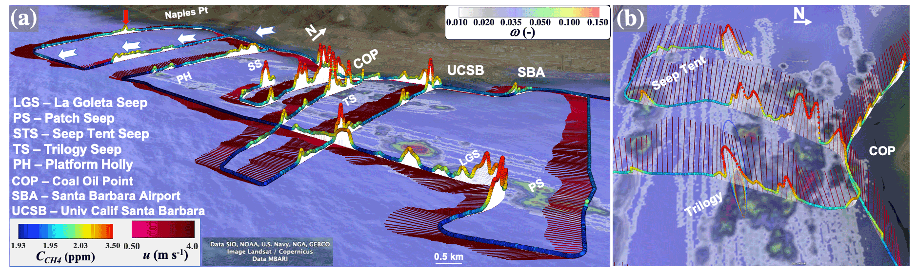
Figure 2(a) Methane, , and wind, u, data for 28 May 2016. White arrows show canyon offshore flow. Red arrows show unmapped seepage to the west of the COP seep field. (b) and u show the Gaussian plume model for Trilogy Seep. Sonar return map shown on sea surface. Data key and seep name key in the panel. Displayed in © Google Earth. See Fig. S6 for overhead view.
Plumes are apparent downwind of major seeps, with the largest plume associated with the Trilogy Seep (Fig. 2b). Strong plumes are also evident downwind of the La Goleta Seep and Patch Seep. Notably, the Seep Tent Seep plume was very weak. The Seep Tent Seep was the dominant seep area in the COP seep field from its appearance in June 1973 (Boles et al., 2001) until recent years.
Additionally, the offshore survey identified focused plumes from beyond the extent of the seep field's 2005 sonar map, specifically in the Goleta Bay, which has been noted (Jordan et al., 2020), and offshore Haskell and Sands beaches, an area with abandoned oil wells, and off Naples Point (Fig. 2a, red arrow).
Plume alkane C′ values were determined by the difference between two “background” air samples collected immediately outside the plume and three Trilogy Seep plume air samples. CH4 of THC was 88.5 %, with ethane, propane, and butane at 3.1 %, 4.2 %, and 2.8 %, respectively, with pentane, hexane, and heptane at 1.11 %, 0.13 %, and 0.04 %, respectively (Table 1). Mean THC molecular weight is 19.6 g mol−1 based on a composition weighting. Branched alkanes were detected, with 2-methylpentane and 3-methylpentane comprising 0.21 %, each, as well as simple aromatics, e.g., benzene and toluene, with concentrations of 78 and 18 ppm, respectively.
Table 1Atmospheric plume composition and model atmospheric emissions.
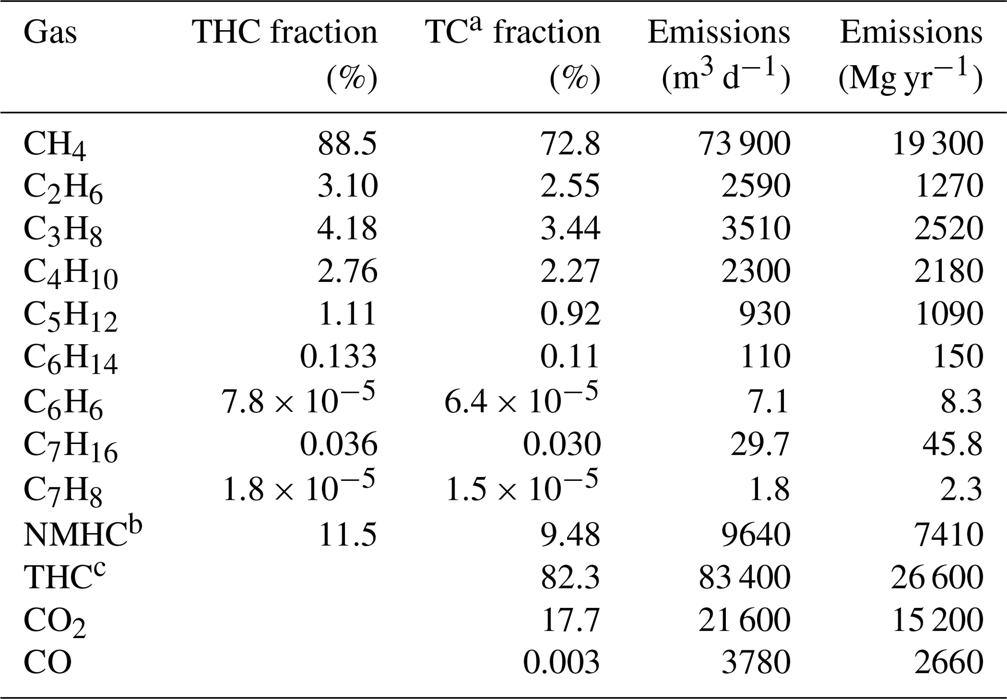
a TC is total carbon and is THC + CO + CO2. b NMHC is nonmethane hydrocarbon and is C2–C7. c THC is total hydrocarbon and is C1–C7.
The observed wet gas fraction, , was 0.11, indicating a thermogenic origin, i.e., greater than 0.05 (Abrams, 2017) – and thus derived from marine organic materials. Although the olefins ethene and ethyne were detectable at 0.02 % and 0.004 %, respectively, butene was not detected. These olefins primarily derive from microbial processes (Abrams, 2017); thus, the ethane ethyne ratio of 6200 strongly indicates a thermogenic source (Bernard et al., 2001). Plume atmospheric CO2 was elevated by 12 ppm; thus CO2 was 18 % of total carbon (TC), defined TC = THC + CO2 + carbon monoxide, CO. CO was elevated minimally in the plume, by just 2 ppb. Given that CO2 completely dissolves from bubbles well before reaching the sea surface (Clark et al., 2010), this demonstrates efficient vertical transport of dissolved seep gases to the sea surface.
Plumes for the Trilogy Seeps, La Goleta Seep, and Seep Tent Seep were inverse Gaussian plume modeled to derive emissions for each plume. For the Trilogy Seeps, the average u across the plume was 5.9 m s−1, insolation was full sun, and the source height was set at 25 m based on Trilogy's atmospheric plume being buoyant. Plume model surface concentrations for the Trilogy B plume are shown in Fig. 2b. The other two seeps are far less intense and used a 1 m source height.
E for Trilogy A seep was 1.28 Gg CH4 yr−1 (5600 m3 CH4 d−1), whereas Trilogy B seep and Trilogy C seep contributed 0.06 and 0.07 Gg CH4 yr−1, respectively, for a total of 6200 m3 CH4 d−1. Note, plume origins and the sonar seep bubble plume locations do not precisely match because the sonar map is for near the seabed, and currents deflect the bubble surfacing location, up to ∼ 40 m. La Goleta Seep released 4000 m3 CH4 d−1 and the Seep Tent Seep released 310 m3 CH4 d−1 with almost no surface bubble expression. For comparison, Clark et al. (2010) used a flux buoy, which measures near-surface bubble fluxes, and found Trilogy Seep emissions of 5500 and 4200 m3 THC d−1 and 930 m3 THC d−1 for La Goleta Seep in 2005 and 5700 m3 THC d−1 for the Seep Tent Seep in 2002. During the cruise, surface bubble plumes were not observed for the Seep Tent Seep, although its bubble plume had been a perennial and dominant feature since its appearance. For reference, Clark et al. (2010) reported THC in near-sea-surface bubbles was 91 % CH4.
3.2 West Campus Station
3.2.1 Temporal trends
WCS is 500 m from the coast (to the southwest), at 11 m altitude, and 850 m almost due south of the ∼ 11 m altitude bluffs of Coal Oil Point (Fig. 1). Terrain slopes gently towards the coast to the southwest and towards a lagoon to the south-southeast, rising again to the southeast of the COP bluffs. This flat relief likely has a small to negligible effect on wind speed and direction, although differential land–ocean heating could influence winds. Wind veering is likely for the coast to the east of COP due to the orientation of the coastline and bluffs.
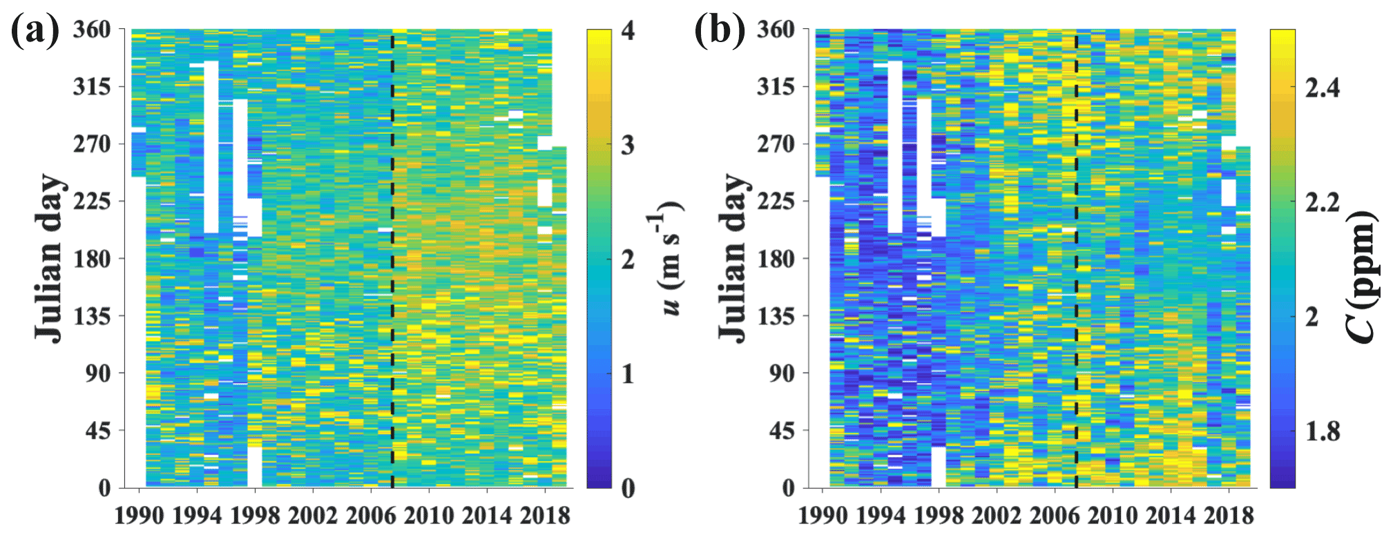
Figure 3(a) Daily mean wind speed, u, and (b) concentration, C. Data key is shown in the figure. The WCS upgrade on January 2008 is shown by a dashed black line. Figure S7 shows the raw dataset.
The WCS improvements in 2008 (Fig. 3 – dashed line) allowed far higher values of C and u (Fig. S7a, b). Comparison of the probability distributions of u and C, φ(u) and φ(C), respectively, before and after the upgrade suggested biases were not introduced (Fig. S7c, d). Specifically, changes in the average and median values and in the baseline after 2008 were from better measurement of higher-value events (gusts and short positive C anomalies).
Significant daily, seasonal, and interannual variations are apparent in the day-averaged u and C (Fig. 3). The calmest season is late summer to fall, whereas spring is the windiest and most variable due to synoptic systems (Fig. 3a). Winds have strengthened since a minimum in 1995–1996, more so for the seep directions, with stronger winds becoming more frequent and more so for summer than winter (Figs. S8, S9).
Trends in C reflect trends in both seep field emissions and ambient C. C is higher in fall and spring (Fig. 3b). Given that stronger winds decrease C from seep emissions through dilution, this suggests the seasonal variation in C underestimates the seasonal variation in emissions. Several studies have shown increased emissions under higher wave regimes (storminess), reviewed in Leifer (2019) and proposed to result from wave pumping. Storms increase evasion from higher wave turbulence and breaking-wave bubbles, which sparge dissolved CH4 and other trace gases as deep as the seabed in shallow (< 100 m) waters (Shakhova et al., 2010b). Note, u, θ, and C′ correlate with time of day. For example, north generally reflects weak (offshore) nocturnal winds with no seep contribution.
3.2.2 Spatial heterogeneity
Calculating the angular-resolved average C, Cave(θ), for the complete dataset with respect to θ shows the highest C is from the main seep field direction (155–250∘, Fig. 4). For the seep directions, Cave(θ) was poorly fit by a single Gaussian function but well fit (R2=0.997) by two Gaussian functions with peaks at 178 and 198∘ corresponding to the Seep Tent and Trilogy Seeps' directions, respectively (Fig. 4a, b). Notably, the fit residual showed a linear increasing trend, , of 0.17 ppb per degree from 180 to 210∘ (Fig. S9b) consistent with evasion from a dissolved downcurrent plume that drifts west-northwest along the coast (Leifer, 2019).
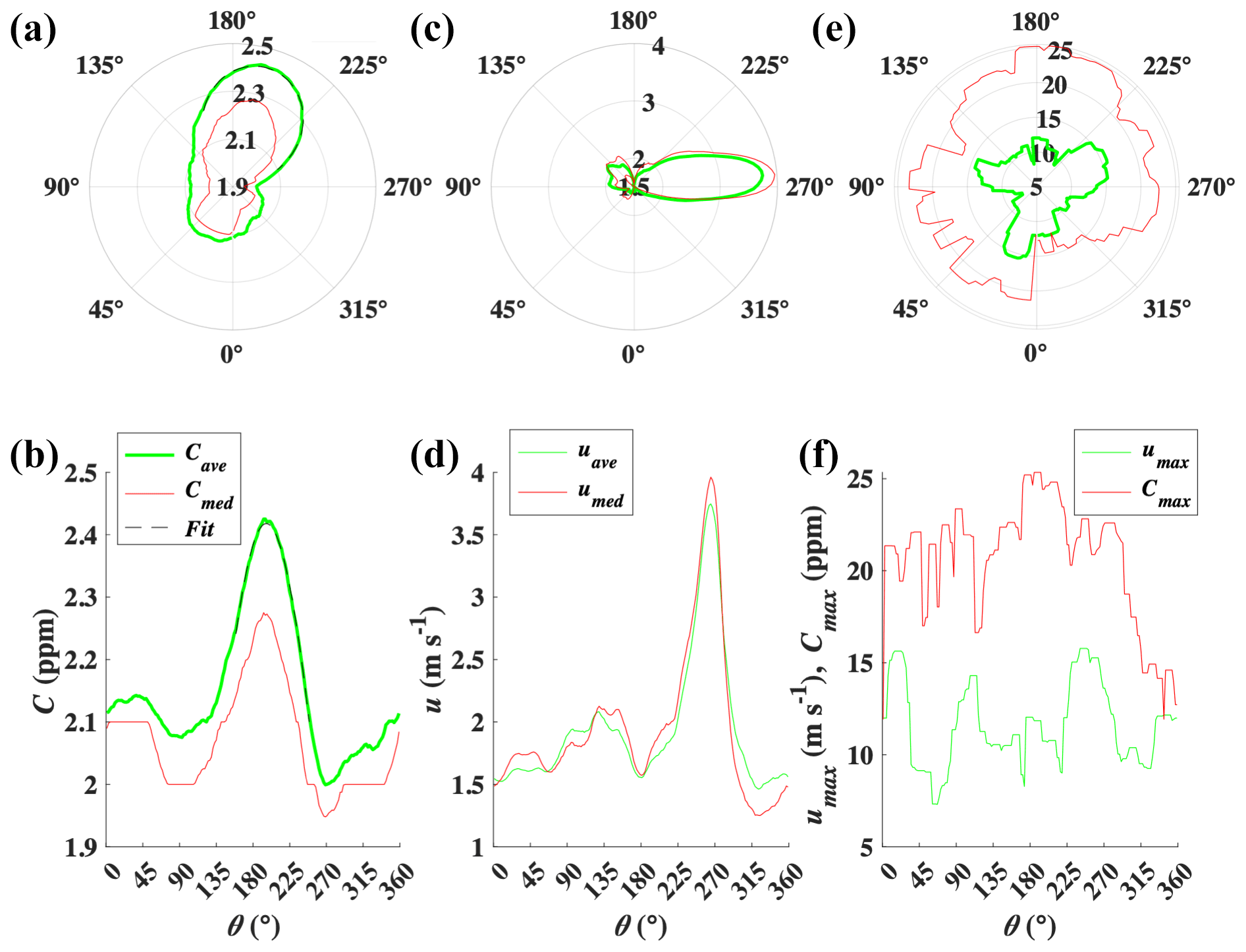
Figure 4(a, b) Concentration, C, versus wind direction, θ, 1990–2021 for average, Cave(θ), and median, Cmed(θ), and fit to Cave(θ) for 155 < θ < 250∘. Data key is shown in panel (b). (c, d) Wind speed, u, average, uave(θ), and median, umed(θ). Data key is shown in panel (d). (e, f) Maximum C, Cmax(θ), and wind speed, umax(θ). Data key is shown in panel (f). Polar plot oriented as at WCS facing the COP seep field.
The average C anomaly, , was calculated from the average of CObs(θ), after Eq. (1), with terrestrial anthropogenic sources from the north to northeast removed. The minimum in CObs(θ) was at 270∘, a direction with no mapped seepage that is also beyond the dissolved plume's approximate shoreward edge. Figure 4a and b show CObs(θ) before removal of terrestrial emissions, which do not overlap in any significant manner with seep field emissions.
There is a strong, focused peak in Cmax(θ) at θ∼ 190∘ (Fig. 4e, f), close to the Seep Tent Seep direction, 198∘ (Table S3), which is fairly isolated on the offshore seep trend (Fig. 1). This peak also is close to the direction of Tonya Seep on the inshore seep trend and close to the small, unnamed area of seepage to the west of Trilogy Seep on the Red Mountain Fault trend. The θ-resolved maximum C(θ), Cmax(θ), remains elevated through ∼ 270∘, far west of the Cave(θ) peak at ∼ 200∘. This strongly suggests that the seep field extends further to the west-northwest than current maps denote. These data cannot be explained by dissolved plume outgassing, which would affect Cave(θ) but not Cmax(θ).
C(θ) enhancements for non-seep directions (Fig. 4a, b) show a peak at ∼35∘, corresponding to the direction of a commercial center amid suburban development. This could result from terrestrial seepage and natural gas pipeline leakage and/or THC emissions from communities and traffic.
Neglecting synoptic systems, topographic forcing from the east–west Santa Ynez Mountains means that the strongest winds are the prevailing westerlies (Fig. 4c, d). North winds (320–15∘) are largely weak, as are winds from due south; however, the sea breeze strengthens winds rapidly away from due south. θ peaks in the maximum winds (1 min sustained), umax(θ), correspond to the west and east peaks in uave(θ) with strengths up to 16 m s−1. Interestingly, there are also strong north (0–30∘) winds or downslope flow, termed sundowner winds, a highly localized and infrequent phenomenon. The overlap of umed(θ) and uave(θ) shows winds are largely normally distributed.

Figure 5(a) Wind direction, θ, and wind speed, u, resolved probability distribution, φ(θ,u), and (b) concentration probability distribution, φ(θ,C), for 1990–2016. The white dashed line shows the edges of the seep field. Data key is shown in the figure.
The median C, Cmed(θ), and average C, Cave(θ), have similar shapes, albeit with lower values at all θ (Fig. 4a), indicating C is not normally distributed. This is shown in the wind-direction-resolved wind speed probability distribution, φ(θ,u) (Fig. 5a), defined such that
φ(θ,u) is very narrow (y axis) for the northeast (∼ 45∘) where winds are largely weak and broad for the east-southeast (70–135∘) and the prevailing westerlies (250–280∘). The east-southeast distribution skews to the south (stronger winds extend further from the south – offshore), whereas the prevailing westerly wind distribution skews to the northeast as does the coastline.
In the seep direction, φ(C,θ) extends to much higher values than from non-seep directions (Fig. 5b). φ(C,θ) is asymmetric, with θ extending further to the west than the seep field extent (240∘) and then decreasing more abruptly than the decrease to the east. This asymmetry is expected given the seep field's asymmetric orientation relative to WCS (eastern seepage is more distant). Emissions beyond the field's mapped western edge arise from downcurrent plume outgassing and potentially contributions from unmapped seeps.
3.2.3 Seep field diurnal emissions cycle
C and u for the seep field direction, useep and Cseep, respectively, follow diurnal patterns that are not the same as the overall diurnal pattern due to the wind direction constraint and because Cseep depends on useep. The dependency arises because higher u dilutes emissions, decreasing C, but higher u also increases dissolved plume evasion and bubble-mediated emissions from higher swell (after a delay for wave build-up). Diurnal winds in coastal regions feature a shift between weak nocturnal offshore winds that veer to onshore winds in the morning – the sea breeze circulation. This was explored in time- and direction-segregated u and C and explored for seep direction-averaged useep and Cseep for 90–270∘ (Fig. 6). Data were segregated by θ for pre- and post-2008 (when station improvements facilitated better wind characterization, particularly for night winds, which are seldom from the seep field direction; see Fig. S10 for 1991–2007). u(θ,t) and C(θ,t) were 2D Gaussian kernel smoothed with a one-bin standard deviation (contours based on a three-bin standard deviation) by the imgaussfilt.m algorithm (MATLAB, MathWorks, MA) after interpolating the calibration data gap 24:00–01:00 LT (local time).
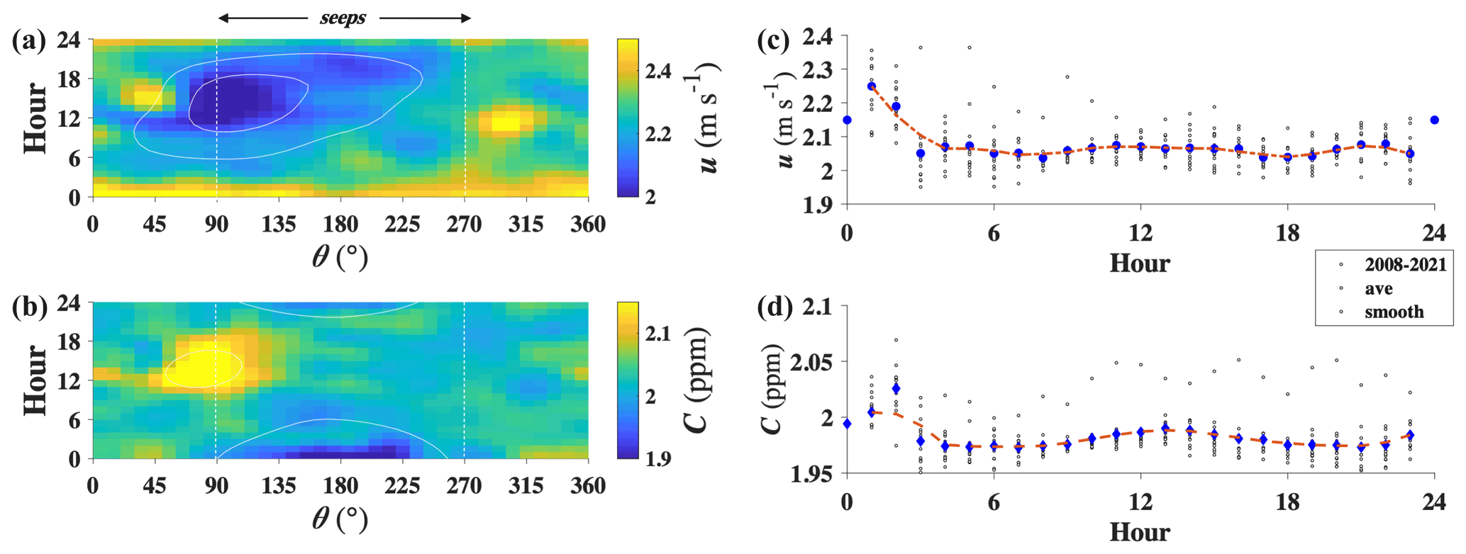
Figure 6(a) The 2008–2021 hour and wind direction, θ, resolved wind speed, u, and (b) concentration, C. (v) Hourly-resolved seep direction (90–270∘), wind speed, u, and (d) concentration, C, averaged for individual years and 3-year smoothed. Data key is shown in the figure. Midnight data are missing due to daily calibration.
Early morning (01:00–03:00 LT) useep is stronger because typical nocturnal winds are northerlies (land breeze), coming from the south largely during storms. These are accompanied by elevated Cseep implying greater emissions despite enhanced dilution from stronger winds. The minimum in both useep and Cseep occurs in the early morning (04:00–08:00 LT), with both increasing slightly through midday (∼ 12:00 LT). Cseep follows an afternoon trend of an overall decrease to a minimum at ∼ 20:00 LT before increasing into the late evening.
Underlying these trends are complex temporal spatial patterns. C for the north to northeast reaches a maximum around noon, whereas u peaks around 16:00 LT. C for the east is low in the morning, reaching a peak in the afternoon and likely reflecting terrestrial sources. This pattern in C(t,θ) extends to nearly 130∘. Beyond the seep field's western edge, u is elevated from the prevailing direction (270∘), with C elevated throughout the morning. There is also a short-lived peak in u around noon at ∼ 300∘, which corresponds to a short period when C is depressed. These could be consistent with wave development time, transport time, and sparging of the downcurrent plume; however, interpretation based on these patterns is largely speculative.
3.3 Overall seep field emissions
3.3.1 Overall emissions
Average atmospheric emissions, EA, for 1990–2020 were derived by an iterative Gaussian plume model, initialized with the 2005 sonar map (Fig. 7a). An emissions sensitivity study on the effect of grid resolution was conducted for resolutions from 11 to 225 m and a 22/56 m hybrid grid (Fig. S3). Simulation turbulence parameters and stability class were for moderate insolation (Fig. S2) and used a 250 m BL, typical of Santa Barbara Channel marine values (Rahn et al., 2017; Edinger, 1959). Simulation angular resolution was 2∘ (Hanna et al., 1982). Simulations were run iteratively until convergence, typically within five iterations (Fig. S11). Sensitivity studies found the distance weighting function, K(r,θ), was linear (Fig. S12).
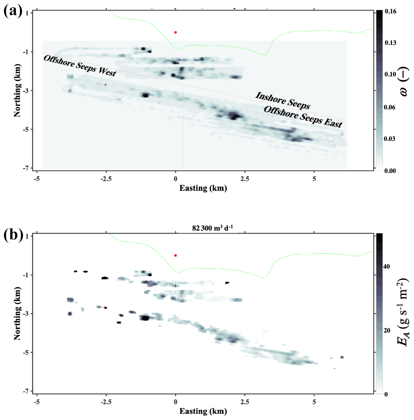
Figure 7(a) Sonar return, ω, gridded at 22 m resolution. (b) Atmospheric emissions, EA. The West Campus Station (red dot) is at the coordinate system origin. The green line is the coastline.
Simulations could not reproduce observations in the Platform Holly direction (). Thus, a source was added for the platform area, which improved simulation–observation agreement in this wind direction. Because significant seep bubble plumes generally are not observed in the platform's vicinity, these emissions could arise from incomplete combustion during flaring.
The model-derived EA for 1990–2020 was 83 400 m3 d−1 (Fig. 7). Use of a composition-weighted THC molecular mass of 19.6 g mol−1 implies 27 Gg THC yr−1. Atmospheric seep gas is 88.5 % CH4, implying seep emissions of 19 Gg CH4 yr−1 (Table 1). Given that CH4 is 73 % of THC, nonmethane hydrocarbon (NMHC: C2–C7) emissions are 9600 m3 d−1, equivalent to 7.4 Gg yr−1, and gaseous emissions are 6.0 Gg yr−1. For reference, 2018 Santa Barbara County reactive organic carbon (ROC) emissions are listed at ∼ 27 t d−1 (9.9 Gg yr−1) (http://www.ourair.org/emissions-inventory, last access: 1 August 2021, SBAPCD). For our analysis, NMHC and ROC are the same. The largest NMHC was propane with emissions of 3510 m3 d−1, followed by ethane at 2590 m3 d−1. The NMHC components of THC are conservative (do not react significantly) on the typical transport timescales from the seep field to WCS (20–30 min).
Seabed emissions, EB, are necessarily significantly greater than EA as EA misses the fraction of emissions that remain in the water column, EW, at least downcurrent close to the fields. There are two notes: first, the model EA includes evasion from the dissolved plume in the area covered by the seep field sonar map. Secondly, the model does not include EA from the dissolved fraction that evades beyond the seep field extent. For the seep field area and near-downcurrent area, Clark et al. (2000) estimated a 50 : 50 air–water partitioning based on a field study, implying EB=167 000 m3 d−1 for 1990–2020 (54 Gg yr−1). A comparison of EA versus ω showed a very steep increase with ω for EA=1–10 g s−1 m−2 with rollover at ω ∼ 0.015 (Fig. S13), which was approximately the noise level (Fig. S4).
Insights were provided by how the model partitioned emissions between different seep areas (Fig. 7). Particularly notable is the model's treatment of the Trilogy Seep area – the second strongest seep area after the Seep Tent Seep during the study period. The model re-assigned Trilogy Seep emissions to seepage to the west, representing Trilogy Seep emissions as unrealistically weaker than other, smaller seeps, such as IV Super Seep. One likely contributor to this re-assignment is wind veering (Fig. S14). Also suggesting wind veering is the model's assignment of strong emissions to the field's eastern and western edges despite weak sonar returns. In a comparison of the Seep Tent Seep and La Goleta Seep areas, the model emphasized the Seep Tent Seep, whereas La Goleta Seep emissions were shifted to inshore seepage. This re-partitioning was greatly reduced for a +10∘ wind veer, which also lessened the strengthening of emissions at the field's western edge relative to sonar. Given the lack of field data between the seep field and WCS on wind veering, further wind veering analysis was not conducted.
3.3.2 Seep field sector emissions
To investigate sub-field-scale emissions, the seep field was segregated into three sectors: inshore, offshore east, and offshore west (Fig. 1). Based on integrating sonar return, ω, inshore seepage contributes 40 % of the field's ω with the offshore seep trend split between 9 % for the west and 51 % for the east. Supporting this comparison is the similarity in the normalized sonar return probability distribution, φn(ω), for the inshore seeps and offshore east seeps (Fig. 8). In contrast, φn(ω) for offshore west seeps differed dramatically despite the similarity in geology along the anticline underlying the offshore seep trend (Leifer et al., 2010). This likely results in part from the interaction between migration and production from Platform Holly. Although the normalized atmospheric emissions probability distribution, φn(EA), for the inshore and offshore seeps is similar over most of the range (except the weakest, EA < 0.02 g s−1), significant differences are evident between offshore east and west seepage. Offshore east seepage is more dispersed and favors weaker seepage compared to offshore west seepage.
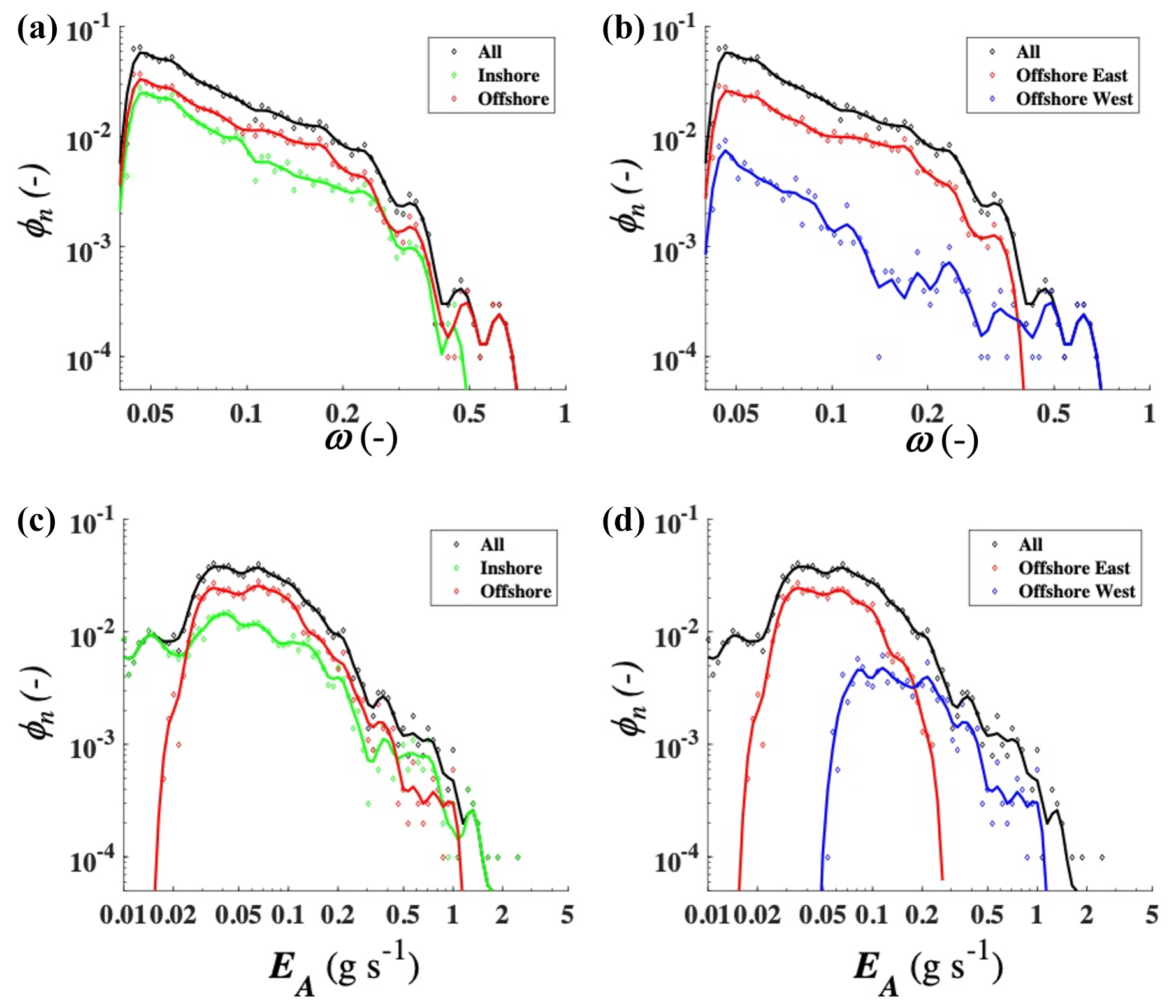
Figure 8(a) Sonar return, ω, and occurrence probability, φn(ω), for all seepage and inshore and offshore seepage and (b) all seepage, offshore east seepage, and offshore west seepage. (c) Atmospheric emission, EA, and occurrence probability, φn(EA), for all seepage and inshore and offshore seepage and (d) all seepage, offshore east seepage, and offshore west seepage. Data key is shown in panels.
The weakest seepage (ω < 0.02) contributed negligibly to overall sonar return and had no notable inshore–offshore φn(ω) difference (Fig. 8). The largest difference is between the strongest seepage (ω > 0.5) for the inshore and offshore seeps. Specifically, there is a strong peak at ω ∼ 0.45 and nothing stronger for the inshore seeps, whereas offshore φn(ω) continued to ω ∼ 0.7. The EA probability distribution, φn(EA), for the strongest inshore seepage was similar to φn(EA) for strong offshore seepage. However, this masked a significant east–west offshore seepage difference. Specifically, φn(EA) for strong seepage was reduced far more for the offshore east seeps than for the offshore west seeps, and the reverse for weak seeps.
The similarities of these distributions suggest that the controlling geological structures (fractures, fault damage zones, chimneys, etc.) are the same for inshore seepage and offshore east seepage, with the primary difference for the strongest seepage in these two sectors being that the inshore Trilogy Seeps provide focused emissions, versus the offshore east La Goleta Seeps being comparatively dispersed and far oilier. Note, these seep areas are of similar strength.
Although ω is not EA, EA followed the 40 : 60 partition in ω between inshore and offshore seepage. Interestingly, the EA partitioning between the offshore east and offshore west differed significantly from sonar partitioning, with 21 % of EA from offshore west and 38 % from offshore east. This greatly accentuated the EA Seep Tent Seep area. In part, this arises from a diurnal cycle bias – WCS observes the offshore west seeps for afternoon to evening westerly winds, which are stronger, whereas WCS observes the offshore east seeps when winds are weaker, earlier in the day (Fig. 6b). Winds also increase bubble emissions from wave hydrostatic pumping and dissolved gas evasion. Also potentially contributing is saturation of ω for very high-bubble-density bubble plumes, primarily for the Seep Tent Seep and Trilogy Seep (Leifer et al., 2017). Saturation would imply an under-estimate of ω for the strongest seep areas' emissions, which are for the west offshore seepage, altering the west : east ω ratio (9 % : 51 %).
3.3.3 Uncertainty and emissions sensitivity
Given the number of sources with poorly characterized variability, uncertainty is best assessed by Monte Carlo simulations; however, this was unfeasible due to the simulations' computational demands. Thus, emissions uncertainty was investigated by sensitivity studies (Fig. 9). Where data were available, uncertainty due to a specific parameter was estimated from the data. Specific parameters studied included sonar resolution; angular resolution, δθ; wind speed, u; concentration anomaly, C′; boundary layer height, BL; wind veering, ψ; spatial northing offset, Y; and the inshore and offshore seepage partitioning, ζ. Sensitivity study details are presented in Sect. S7.4.
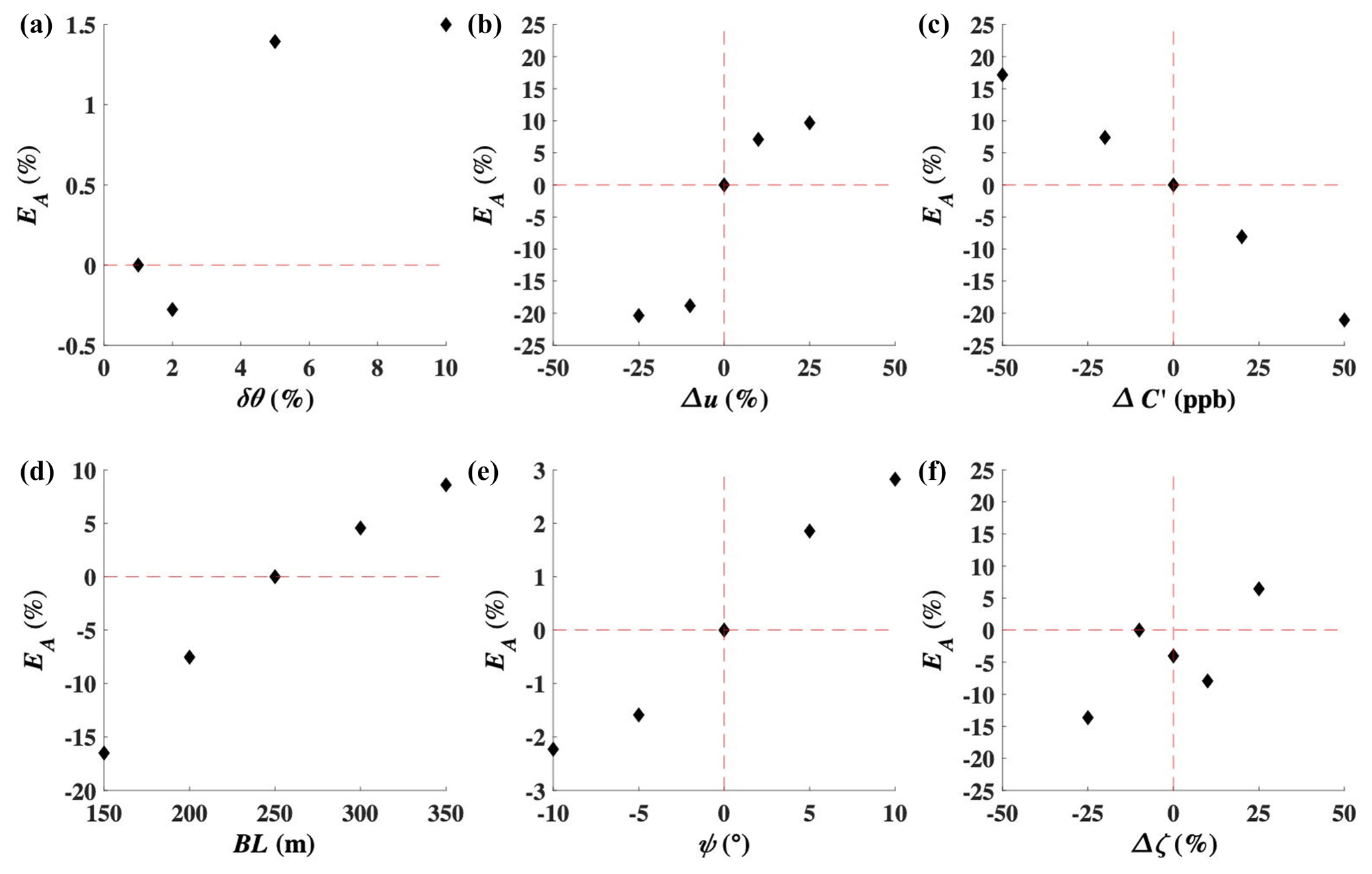
Figure 9Atmospheric emissions, EA, sensitivity to uncertainty in (a) model angular resolution, δθ, (b) wind speed variation, Δu, (c) concentration anomaly variation, ΔC′, (d) boundary layer thickness, BL, (e) wind veering, ψ, and (f) inshore–offshore partition variation, Δζ. Note that there are different units in different plots. See text for details.
The contribution to uncertainty from δθ, C′, ψ, and spatial offsets within the seep trends were minimal – just a few percent or less. Moderate uncertainty was identified for BL and ζ. For example, for BL ranging from 150 to 350 m, mean EA uncertainty was 6 %. Although u has strong sensitivity, combined with BL its sensitivity is weak as u opposes BL – lower u corresponds to higher BL. There remains uncertainty, though in the value of BL, which was not measured. Assessing uncertainty in ζ was more challenging as there are no verification data on variability in the EA partitioning between the inshore and offshore seep trends. The mean EA uncertainty for −50 % < ζ < 50 % is 11.5 % from a polynomial fit. Still, the consistency in seepage location between sonar surveys spanning decades (Leifer, 2019) suggests only modest changes in ζ over the multi-decade time period of model averaging. Total uncertainty was taken as 15 % based on the sum of uncertainty in BL and ζ, each averaged to the nearest 5 %.
3.4 Ellwood Field emissions
C(θ) increases to the northeast with a peak at 290–320∘ corresponding to the direction towards abandoned wells off Haskell Beach (Fig. 10). Emissions from this area – either from natural seepage or leaking wells – were noted in the offshore survey data near Haskell Beach (Fig. 2a). Additionally, Cmax(θ) shows a 22 ppm peak in this direction, well above Cave(θ) (Fig. 4f). This is consistent with transient releases from natural seep and/or abandoned well emissions.
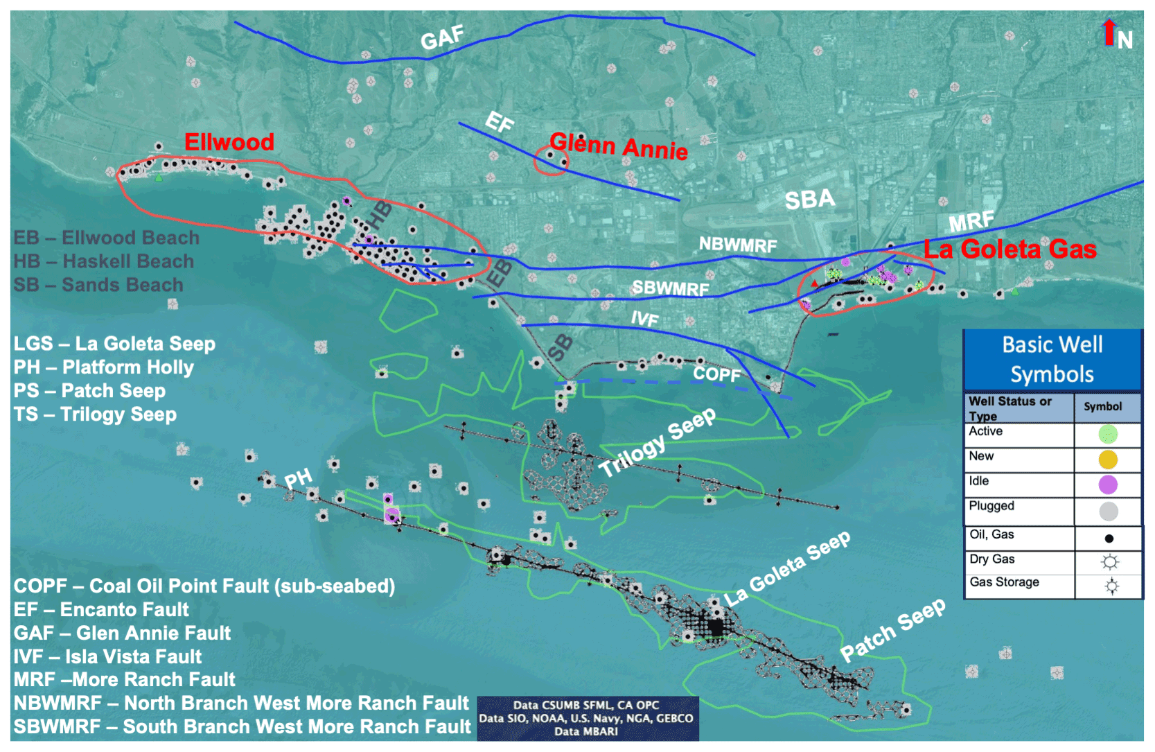
Figure 10Map of the Goleta Plains oil and gas fields, wells, and the Coal Oil Point (COP) seep field. Grey hatching shows the 1995 field extent, and green outlines the 1940 field extent from Leifer (2019). Field locations are from Olson (1983). Well data are from CDOGGR (2018). Faults are from Minor et al. (2009). Seep names are informal. Data keys are shown in the panels. Shown in the © Google Earth environment.
Ellwood field production continued through the 1970s, with wells drilled into the geological structures that allowed oil accumulation (Olson, 1983), including faults that provide migration pathways (Leifer et al., 2010). There are many abandoned wells from these oil fields and others on the Goleta Plains, beaches, and shallow near-coastal waters to the west-northwest of WCS (offshore Haskell Beach and onshore around Naples Point). Currently, active wells are only found at the La Goleta gas field (a natural gas storage field), east of WCS.
Faults associated with these anticlines provide migration pathways and are aligned approximately with the coast in a series of roughly parallel faults extending onshore (Minor et al., 2009). The onshore–coastal Ellwood field (northwest of the South Ellwood field) sources from the primarily sandstone Vaqueros Formation (Olson, 1983), whose main trap is an anticline at the western edge of the North Branch Western More Ranch Fault (NBWMRF). Offshore seepage tracks some of these faults; e.g., the Isla Vista Fault trend corresponds to an offshore seep trend in Goleta Bay that includes the Goleta Pier Seep, whereas wells follow the NBWMRF trend offshore of Haskell Beach.
4.1 Atmospheric seep field observations
4.1.1 Air quality station
A range of approaches are available to evaluate marine seepage CH4 emissions. Specifically, in situ approaches include direct capture (Leifer, 2015; Washburn et al., 2001), fluid flow measurements (Leifer and Boles, 2005), video (Leifer, 2015), and remote sensing that include active acoustics, i.e., sonar (Hornafius et al., 1999), dissolved in situ CH4 (Marinaro et al., 2006), and passive acoustics (Wiggins et al., 2015). Remote sensing is the best approach for long-term monitoring to capture shifts in emissions between vents. To date, only sonar remote sensing has provided quantitative seep plume (seabed) emissions (Hornafius et al., 1999). Notably, sonar ranges are up to a few hundred meters, far less than the size scales of many seep fields, whereas high power demands typically require a cabled observatory for long-term observations.
This study demonstrated that air quality station data can provide the long-term continuous data needed to capture seasonal variations, including emissions during storms and transient events, which field campaigns likely miss. For example, sonar surveys are generally scheduled during summer when seas are calmer and winds are more predictable and when seepage is weakest (Fig. 3), however not during storms when emissions are likely enhanced.
The approach presented in this study derived atmospheric trace gas emissions from long-term air quality and meteorology data for a dispersed area source that is constrained by sonar seepage maps. This approach can be extended to terrestrial seepage if the source can be constrained spatially (e.g., by geology), although nearby anthropogenic sources may complicate emissions assessments. Other terrestrial sources such as landfills, O&G production fields, or industrial sites – if spatially constrained – could be addressed by this approach, particularly if isolated from other confounding sources. The use of cavity-enhanced absorption spectrometers that can speciate gases like CH4 and C2H6 could enable discrimination of some confounding sources as well as better characterization of emissions. Although onshore stations can address nearshore seepage, further offshore seepage could be addressed by a moored station. Moored stations could also include in situ aqueous chemical sensors and current measurements.
4.1.2 In situ atmospheric surface surveys
Atmospheric emissions were assessed for three seep areas – a zone of focused seepage – by an atmospheric in situ survey approach wherein downwind data are collected orthogonally to the wind direction in a transect that spans the plume (background to background on the plume's edges). This approach was developed for terrestrial sources (Leifer et al., 2018b) yet remains unused for offshore marine seepage, which are often area sources. In this study, this was addressed by gridding the area source and treating each grid as a far-field point source. Gaussian plume inversion requires distant point source(s), i.e., far field. Downwind in situ transects of three strong seep areas were all well-characterized by the Gaussian plume model.
One advantage of atmospheric surveys is rapidity – a single transect of a few minutes is sufficient to derive emissions for a seep area. In comparison, a flux buoy survey can require many hours to a day (Clark et al., 2010), during which forcing factors (waves, tides, etc.) change significantly. Seep area sonar surveys are also rapid (Wilson et al., 2015), allowing a combined sonar and atmospheric survey to repeat characterize emissions and sea–air partitioning within a few hours. With respect to the entire COP seep field, whereas a sonar survey requires 2 to 3 d (Leifer et al., 2010), a downwind atmospheric survey is far more rapid, requiring perhaps an hour. This allows repeat field emissions measurements over a tidal cycle.
4.2 Seep field emissions
4.2.1 Total emissions
To date, only two estimates of COP seep field seabed emissions, EB, have been published. Hornafius et al. (1999) estimated EB=1.5 × 10⁵ m3 d−1 (64 Gg yr−1) based on sonar surveys covering 18 km2 from November 1994–September 1996, collected during the summer to late fall seasons. This value excluded Seep Tent collection. A 4.1 km2 sonar survey in August–September 2016 estimated EB=24 000 m3 d−1 (Padilla et al., 2019), significantly lower. In part, this arises from field subsampling, but could also arise from long-term changes. Notably, neither study addressed temporal variability. The sonar surveys occurred in summer and fall when seepage activity is at a minimum, whereas winter and early spring feature much higher activity associated with storms (Bradley et al., 2010).
Hornafius et al. (1999) used an engineered bubble plume to calibrate emissions, an approach also used in Leifer et al. (2017). Due to technology limitations at the time, the strongest seepage was clipped/saturated, i.e., underestimated, and the survey did not cover shallow seepage. Thus, the Hornafius et al. (1999) emissions estimate is a lower limit for summer–fall emissions. The Padilla et al. (2019) survey was calibrated by an inverted seep flux buoy suspended at 23 m. This differs significantly from the seep flux buoy measurement approach reported in Washburn et al. (2001), which was collected in surface drift mode. Surface drift mode ensures a horizontal orientation for the buoy and an absence of lateral velocity difference between the capture device and currents – either of which decreases capture efficiency from 100 %, biasing derived emissions low. Further, the Padilla et al. (2019) survey was calibrated 1 month after the sonar surveys, whereas the 1995 engineered plume calibration by Hornafius et al. (1999) was contemporaneous. The Hornafius et al. (1999) approach accounts, in part, for dissolution between the seabed and survey depth window – it uses air rather than CH4, which dissolves more slowly than CH4. Dissolution losses for CH4 between the seabed and the depth window can be addressed by a numerical bubble model (Leifer et al., 2017).
The Gaussian plume model-derived EA was 8.3 × 10⁴ m3 d−1. Based on the Clark et al. (2000) assessment that half the seabed seepage reaches the atmosphere, EB=1.7 × 10⁵ m3 d−1; very similar to EB=1.5 × 10⁵ m3 d−1 from Hornafius et al. (1999). This agreement is coincidental as it neglects seasonal and interannual trends. For example, Bradley et al. (2010) found 1994–1996 emissions were well below the average for 1990–2008, increasing significantly after 2008.
4.2.2 Methane and nonmethane hydrocarbon emissions
Analysis of atmospheric samples provided a picture of the complexity of atmospheric emissions that arises from the multiple pathways underlying atmospheric emissions. Specifically, as bubbles rise, they lose lighter and more soluble gases faster (deeper in the water column), leading to differences between evasion from dissolved gases and direct bubble transport (Leifer and Clark, 2002). Thus, bubble-mediated transport enhances larger alkanes relative to smaller alkanes, leaving more of the smaller alkanes in the water column. For strong seeps, bubble plumes are associated with strong upwelling flows (Leifer et al., 2009), which transport dissolved gases to the sea surface where they outgas. Additionally, oil (as droplets and bubble coatings) enhances alkane transport due to slower dissolution and diffusion of larger alkanes through oil.
Atmospheric plume concentrations were 11.5 % NMHC and 88.5 % CH4, very similar to Hornafius et al. (1999), who referenced the Seep Tent composition (88 % CH4, 10 % NMHC, and 2 % nitrogen) as very similar to the reservoir composition. Note, Clark et al. (2010) observed near-sea-surface bubbles from Trilogy with 5.7 % to 7.9 % NMHC and 52.4 % to 79.7 % CH4, demonstrating significant partitioning. The similarity between the atmospheric and seabed composition demonstrates efficient dissolved gas transfer to the sea surface despite the difference in the bubble composition.
COP seep field seabed emissions are orders of magnitude greater than typically reported for other seep areas, e.g., the summary in Römer et al. (2017) where emissions for 12 different seep areas including sites in the North Sea, Pacific Northwest, Gulf of Mexico, and other areas were 2–480 t yr−1, multiple orders of magnitude less than COP seep field seabed emissions. Römer et al. (2017) used a bubble model for Dogger Bank seepage in the North Sea to estimate emissions for observed atmospheric CH4 plumes. The model estimated direct atmospheric bubble-mediated emissions of 21.7 t yr−1, 20 % of seabed emissions. For the Tommelieten Seeps (in 70 m water), Schneider Von Deimling et al. (2011) estimated 4 % of the 0.024 Gg CH4 yr−1 seabed emissions, i.e., ∼ 1 Mg CH4 yr−1, reached the atmosphere by bubble-mediated transfer. Schneider Von Deimling et al. (2011) used a bubble model based on an assumed bubble size and neglected diffusive flux. These diffusive fluxes include bubble dissolution in the wave-mixed layer in the local area. A few studies have directly measured atmospheric fluxes by an air–sea gas transfer model. For example, Schmale et al. (2010) found seep air fluxes of 0.96–2.32 nmol m−2 s−1, much higher than the ambient Black Sea flux of 0.32–0.77 nmol m−2 s−1. In the Black Sea, ambient emissions arise from microbially produced CH4 in shelf and slope sediments (Reeburgh et al., 1991). Di et al. (2019) estimated 7.7 nmol m−2 s−1 for the shallow South China Sea based on an air–sea gas transfer model. If we disperse COP seep field atmospheric emissions of 1.15 × 10⁹ M yr−1 over the ∼ 6.3 km2 of 25 × 25 m2 bins with emissions, we find 5.7 µM m−2 s−1, 3 orders of magnitude greater.
Recent estimates of total global geo-CH4 sources from a bottom-up approach are 45 Tg yr−1, with submarine seepage contributing 7 Tg yr−1 (Etiope and Schwietzke, 2019), implying that the COP seep field contributes ∼ 0.27 % of global submarine emissions. However, an estimate of pre-industrial CH4 emissions (not confounded with fossil fuel production emissions) based on ice core 14CH4 suggested 1.6 Tg yr−1 of geo-CH4 emissions (Hmiel et al., 2020). This estimate, if accurate, would imply the COP seep field contributes an astounding 1 % of global seep emissions (submarine and aerial) and is difficult to reconcile with the COP seep field and seepage estimates for other high-emission seep fields. For example, atmospheric CH4 emissions for the Lusi hydrothermal system were estimated at 0.1 Tg yr−1 (Mazzini et al., 2021), a hotspot in the Laptev Sea was estimated at 0.9 Tg yr−1 into shallow seas (Shakhova et al., 2010a), and emissions for the East Siberian Arctic Sea using eddy covariance were estimated at 3.0 Tg yr−1 (Thornton et al., 2020).
COP seep field C2H6 emissions were 1.27 Gg C2H6 yr−1. For reference, this is 11 % of the 11.4 Gg C2H6 yr−1 in 2010 for the South Coast Air Basin (SCAB), which includes Los Angeles (Peischl et al., 2013). Globally, Simpson et al. (2012) and Höglund-Isaksson (2017) found 11.3 and 9.7 Tg C2H6 yr−1 in 2010, respectively. C2H6 has been increasing since 2010 due to increased O&G production emissions (Helmig et al., 2016). Globally, seeps are estimated to contribute 2–4 Tg C2H6 yr−1 (Etiope and Ciccioli, 2009) and 2.2–3.5 Tg yr−1 from ice cores (Nicewonger et al., 2016). This suggests the COP seep field contributes 0.03 %–0.06 % of global seep C2H6 emissions.
Seep THC was 4.2 % C3H8, implying emissions of 2.5 Gg C3H8 yr−1. Global propane emissions are 10.5 Tg yr−1 (Pozzer et al., 2010), with 1–2 Tg yr−1 estimated for seeps (Etiope and Ciccioli, 2009). This suggests the COP seep field contributes 0.05 %–0.1 % of the global seep budget. Oceans are estimated to contribute 0.35 Tg C3H8 yr−1 (Pozzer et al., 2010), less than geological seepage contribution.
Based on an evaluation of the COP seep field emissions with respect to global seep ethane and propane emissions, the COP seep field contribution to global geo-CH4 emissions is consistent with recent global geo-gas CH4 emissions estimates of 45 Tg yr−1 (0.04 %) (Etiope et al., 2019) and not the significantly lower pre-industrial estimates of global geo-CH4 emissions, e.g., 1.6 Tg yr−1 (1.15 %) (Hmiel et al., 2020).
Global butane emissions are 14 Tg C4H10 yr−1 (Pozzer et al., 2010), higher than ethane and propane. COP seep field butane (C4) and pentane (C5) emissions were 2.2 Gg C4H10 yr−1 and 1.1 Gg C5H12 yr−1, respectively, with combined C2–C5 emissions of 7.1 Gg yr−1, compared to 65 Gg yr−1 from the entire SCAB, i.e., COP seep field contributes ∼ 5 % in the SCAB. COP C2–C5 emissions are significantly above those of the La Brea area, estimated at 1.7 Gg yr−1 (Weber et al., 2017). Note, COP seep field atmospheric C2–C5 emissions certainly are larger, potentially significantly, as larger alkanes are also emitted from oil slicks but were not considered for this study, and furthermore, the atmospheric plume from the slicks was not sampled for this study.
Both benzene and toluene were detected with estimated emissions of 8300 and 2300 kg yr−1, respectively. These emissions are likely underestimates, potentially significantly, due to neglecting the oil slick evaporation contribution. Both gases are of significant health concerns, as are alkanes like pentane and hexane.
4.3 Downcurrent emissions
The seep field concentration, C′(θ), anomaly was centered at θ ∼ 200∘ – the Seep Tent Seep (198∘ – Table S3), and was well-described by a dual Gaussian function (Fig. 4b). This was surprising given that the seep field is asymmetric with respect to a 200∘ axial line from WCS to COP. Underlying this seeming discrepancy is that WCS winds are weakest from due south and strongest from the west (prevailing) and also stronger to the east-southeast (Fig. 4c).
The residual of the Gaussian fit increased in the downcurrent direction (Fig. S9b), consistent with evasion from the downcurrent dissolved plume and seepage from this area. The dissolved plume roughly follows the coast, extending as far as ∼ 280∘ from WCS due to the coastline shift from northwest to west around Haskell Beach (Fig. 10), ∼ 30∘ beyond the seep field's sonar-mapped western edge (Fig. 1). As prevailing winds are westerlies (paralleling the coastal mountains), downcurrent plume evasions decrease with distance due to dispersion and as surface waters become depleted by evasion. Evasion increases nonlinearly with u, particularly for winds that include wave breaking (Nightingale et al., 2000); however, higher winds also dilute emissions. Note, there are no mapped seeps in this area.
Dissolved plume emissions also likely occur from east of the field, leading the model to emphasize seepage at the field's eastern extent, too. Specifically, strong prevailing afternoon westerly surface winds drive a near-surface dissolved plume eastwards. When these westerly winds calm down late in the evening, leaving the plume of dissolved seep gases to the east. Morning easterly winds then transport evasion from this east-displaced dissolved plume towards WCS. Additionally, it is also possible that the COP seep field extends further east than mapped in sonar surveys, at least during some seasons.
4.4 Focused seep area emissions
Trilogy Seep area emissions were estimated at 6200 m3 CH4 d−1 in May 2016. For comparison, Clark et al. (2010) found 5500 and 4200 m3 THC d−1 (4900 and 3700 m3 CH4 d−1) for Trilogy Seep as measured by a flux buoy for near-surface bubble fluxes in September 2005. Note, the plume inversion approach also includes outgassing of near-surface waters that have enhanced from plume dissolution, which the flux buoy approach does not include. Although Clark et al. (2010) found surface bubbles had undetectable CO2, the atmospheric plume's CO2-to-CH4 concentration ratio was comparable to the seabed bubble concentration ratio. This demonstrates efficient upwelling flow transport of seabed water to the sea surface where dissolved gases evade near where the bubble plume surfaces. This near-bubble-plume evasion contributes to the atmospheric plume. Note, these emissions neglect downcurrent emissions. A 50 : 50 atmosphere : ocean partitioning suggests 2016 Trilogy Seep emissions were ∼ 40 % lower than in 2005 – a difference within the difference between the two 2005 Trilogy Seep measurements by Clark et al. (2010).
In contrast, agreement was very poor for the Seep Tent Seep, for which Clark et al. (2010) mapped emissions of 5700 m3 d−1 (5000 m3 CH4 d−1) in November 2002, whereas this study found 310 m3 CH4 d−1. This discrepancy was readily apparent with almost no visible surface bubble expression in May 2016, whereas the Seep Tent Seep has been a perennial feature since its appearance. The absence of more than a few scattered bubbles at the sea surface (Ira Leifer, personal observation, 2016) – the boil in 2000 was driven by a 1–2 m s−1 upwelling (Leifer et al., 2000) – indicates that most emissions are from evasion. A buoyancy plume associated with the rising oil droplets (thick oil slicks surface above the Seep Tents) as well as CH4 dissolved in the oil are likely transporting the observed, focused CH4 emissions.
This is remarkable given that the seep field's geofluid migration “center” in recent decades has been the Seep Tent Seep (Bradley et al., 2010), which was the largest seep in the field in 2010 (Clark et al., 2010). The Seep Tent Seep consists of emissions not captured by the Seep Tents – two large (33 m square) steel capture tents on the seafloor. For reference, the Seep Tents captured ∼ 16 800 m3 gas d−1 in the early 2000s (Boles et al., 2001). Bradley et al. (2010) found that in WCS data when overall seep field emissions decreased to a minimum in 1995, they were focused on the Seep Tent Seep direction. Note, the Seep Tent Seep was observed first in 1970 as a boil visible from 1.6 km away. The Seep Tent Seep was tented in September 1982 (Boles et al., 2001).
Underlying these observations are several factors. First, the Seep Tent Seep is modern – since 1978 – as it was not mapped in a 1953 seep survey (Leifer, 2019). At the time, it was first reported as a sea boil visible over a kilometer away (Boles et al., 2001). Since installation, overall Seep Tent production has diminished (Boles et al., 2001) by a factor of 3 from 1984 to 1995. Some fraction of this trend could have resulted from the expansion of active seepage beyond the seep tents. Perhaps more significantly, the Seep Tent Seep lies over one of the Platform Holly wells (Leifer et al., 2010; Fig. 3c), creating the potential of linkage between well production (including stimulation) and Seep Tent production and thus Seep Tent seepage (the uncaptured portion).
4.5 Diurnal trend and bias
The diurnal wind patterns typical of the coastal Pacific marine environment are weak offshore (northerly) night winds that shift to the east in the morning and then further shift to the south. In the afternoon they strengthen and shift to prevailing westerlies, continuing to late in the evening (Bradley et al., 2010). Note, WCS seep emissions require winds to “probe or scan” across the seep field and thus miss the strong afternoon prevailing winds when emissions are expected to be higher. This is because higher wind speeds increase sea–air gas emissions of dissolved near-surface gases (Nightingale et al., 2000) and increase emissions from higher hydrostatic pressure fluctuation driven by wave height (Leifer and Boles, 2005). Given that prevailing winds are westerlies, higher afternoon emissions will generally (but not always) drift eastwards, missing WCS.
The diurnal wind pattern from the seep field direction is different from the overall (direction-independent) diurnal pattern. Typical nocturnal winds are quite weak, 1.5–1.7 m s−1 (Fig. 6). The strongest diurnal wind change was from late night to morning, a 20 % decrease. Onshore winds (seep direction) in the middle of the night are from synoptic systems and were associated with the highest C′. Winds increase by a few percent to an early afternoon peak, decreasing through early evening before increasing again later in the night.
The diurnal trend for C from the seep direction followed the diurnal wind cycle, increasing by ∼ 20 ppb and peaking ∼ 2 h later in the day than winds (15:00 LT versus 13:00 LT for C compared to u, respectively). This may reflect the lag in wave development with respect to wind strengthening and transport time. Based on sensitivity studies, the diurnal cycles in u and C correspond to variations of ∼ 7 % and ∼ 9 % in EA.
Although efforts were made to characterize the diurnal cycle from WCS data, WCS data poorly sample the seep field for the higher wind speeds that occur in the afternoon, which are primarily westerlies. Note, nonlinearity in sea–air evasion with u means the model use of average u underestimates EA. Thus, the contribution of the prevailing afternoon winds to diurnal emissions is significantly underestimated from WCS data. It is worth noting, though, that this factor only affects 25 %–33 % of diurnal emissions. As the true diurnal cycle cannot be derived from WCS data, repeat field transects spanning the different phases of a diurnal cycle are needed.
4.6 Future needs and improvements
The sensitivity studies identified areas for improvement and data gaps. These are described in brief below and in more detail in Sect. S8. The largest uncertainty was with regards to partitioning between the inshore and offshore seep trends, which could be determined by a second air quality station, preferably including speciation such as by CEAS analyzers of CH4, C2H6, and C3H8. Further simulations could add grid cells for evasion corresponding to the downcurrent plumes to assess their contribution. The model was limited by available workstation power; however, additional computation power could open improvements such as simulating a range of wind speeds based on the wind speed probability distribution with respect to wind direction, φ(u,θ), e.g., Fig. 5.
Additional fieldwork and data are also needed. Another important sensitivity was to boundary layer height, BL, which varies diurnally and seasonally (Dorman and Winant, 2000) and could be derived from ceilometer data (Münkel, 2007). Another significant concern is afternoon seep field emissions that bypass WCS, which could be addressed by fieldwork and a second air quality station at a different downwind direction from the seep field. Mapping offshore wind fields to characterize wind veering across the seep field is needed to allow simulations to provide insights at the seep area size scale.
In this study, data from an onshore air quality station located downwind of a large marine seep field were analyzed to derive the 3-decade-averaged seep field emissions using an inversion model. The modeled emissions were similar to reported emissions; however, this was coincidental given that prior reported emissions were during a period of field quiescence. Highlighting the significance of the COP seep field, ethane and propane emissions suggest the COP seep field contributes 0.04 % and 0.12 % of the global seep budget, respectively. As a result, COP seep field emissions of 19 Gg CH4 yr−1 are consistent with global geo-gas budgets of 45 Tg yr−1 but inconsistent with significantly lower emissions estimated from ice core isotopic data. Additionally, the approach could be adapted to air quality station data for other sources including terrestrial seeps and production fields if the sources are spatially constrained and isolated from confounding sources.
| NMHC | Nonmethane hydrocarbons |
| O&G | Oil and gas |
| TC | Total carbon |
| THC | Total hydrocarbon |
| WCS | West Campus Station |
| Cave(θ) | Wind-direction-resolved average concentration |
| Methane concentration | |
| Cmax(θ) | Wind-direction-resolved maximum concentration |
| Cmed(θ) | Wind-direction-resolved median concentration |
| WCS observed concentration | |
| Cseep | Concentration in seep directions |
| WCS simulated concentration | |
| uave(θ) | Wind-direction-resolved average u |
| umax(θ) | Wind-direction-resolved maximum u |
| umed(θ) | Wind-direction-resolved median u |
| useep | Wind speed in seep directions |
| BL | Boundary layer height |
| C | Concentration |
| C(t,θ) | Wind-direction- and time-resolved average concentration |
| C′ | Plume concentration anomaly |
| C1–C6 | Concentrations, methane to hexane |
| EA | Atmospheric emissions |
| EB | Seabed (bottom) emissions |
| Ei,j | Grid cells i and j atmospheric emissions |
| EW | Emissions to the water column in the near field |
| i | Grid cell easting index |
| j | Grid cell northing index |
| K(r,θ) | Wind-direction- and distance-resolved correction function to emissions |
| K(θ) | Wind direction varying, distance correction function to emissions |
| r | Distance from WCS to cells i and j |
| R | Residual in C′ after Gaussian functional fit |
| R2 | Correlation coefficient |
| t | Time |
| u | Wind speed |
| u(θ) | Wind-direction-resolved wind speed |
| x, y | Cartesian coordinate system in wind reference frame |
| Y | Northing offset of WCS |
| δθ | Model wind direction angular resolution |
| φ(u) | Wind probability distribution |
| φ(θ,C) | Wind-direction- and concentration-resolved probability distribution |
| φ(θ,u) | Wind-direction- and wind-speed-resolved probability distribution |
| φ(ω) | Sonar return probability distribution |
| φn(EA) | Normalized atmospheric emissions probability |
| φn(ω) | Normalized sonar return probability distribution |
| θ | Wind direction |
| ω | Sonar return |
| ψ | Wind veering |
| ζ | Relative inshore and offshore emissions |
All data needed to evaluate the conclusions in the paper are present in the paper and/or the Supplement and/or were submitted to the Mendeley Data repository (https://doi.org/10.17632/znzhxkftm8.1, Leifer, 2020).
The Supplement contains additional supporting figures and details to complement the paper and an interactive map file as a Google Earth archive of the offshore survey data that are presented in Fig. 2. The supplement related to this article is available online at: https://doi.org/10.5194/acp-21-17607-2021-supplement.
IL developed and conducted the study, analyzed data, and wrote the manuscript. CM analyzed data and edited the manuscript. DRB analyzed air sample data and edited the manuscript.
The authors declare that they have no conflict of interest.
Publisher’s note: Copernicus Publications remains neutral with regard to jurisdictional claims in published maps and institutional affiliations.
We would like to gratefully acknowledge the SBCAPCD for providing data from their ongoing monitoring program and Marc Moritsch and Joel S. Cordes in particular for help with these data and Doug Wilson for the processed sonar data. We recognize the skill and participation of vessel captains Jeff Wright and Tony Vultaggio and appreciate the editorial review by Charlotte Marston, Bubbleology Research International.
This research has been supported by Plains All American Pipeline and the BRI Internal Research and Development fund (IRAD).
This paper was edited by Timothy Bertram and reviewed by two anonymous referees.
Abrams, M. A.: Significance of hydrocarbon seepage relative to petroleum generation and entrapment, Mar. Petrol. Geol., 22, 457–477, https://doi.org/10.1016/j.marpetgeo.2004.08.003, 2005.
Abrams, M. A.: Evaluation of near-surface gases in marine sediments to assess subsurface petroleum gas generation and entrapment, Geosciences, 7, 35, https://doi.org/10.3390/geosciences7020035, 2017.
Bernard, B. B., Brooks, J. M., and Zumberge, J.: Determining the origin of gases in near-surface sediments, AAPG Hedberg Conference, Vancouver BC, Canada, 16–19 September 2001, 1–4, 2001.
Boles, J. R., Clark, J. F., Leifer, I., and Washburn, L.: Temporal variation in natural methane seep rate due to tides, Coal Oil Point area, California, J. Geophys. Res.-Oceans, 106, 27077–27086, https://doi.org/10.1029/2000JC000774, 2001.
Borges, A. V., Champenois, W., Gypens, N., Delille, B., and Harlay, J.: Massive marine methane emissions from near-shore shallow coastal areas, Sci. Rep., 6, 27908, https://doi.org/10.1038/srep27908, 2016.
Bradley, E. S., Leifer, I., and Roberts, D. A.: Long-term monitoring of a marine geologic hydrocarbon source by a coastal air pollution station in Southern California, Atmos. Environ., 44, 4973–4981, https://doi.org/10.1016/j.atmosenv.2010.08.010, 2010.
CDOGGR: Well Finder, available at: https://www.conservation.ca.gov/calgem/Pages/WellFinder.aspx (last access: 1 April 2020), 2018.
Ciotoli, G., Procesi, M., Etiope, G., Fracassi, U., and Ventura, G.: Influence of tectonics on global scale distribution of geological methane emissions, Nat. Commun., 11, 2305, https://doi.org/10.1038/s41467-020-16229-1, 2020.
Clark, J. F., Washburn, L., Hornafius, J. S., and Luyendyk, B. P.: Natural marine hydrocarbon seep source of dissolved methane to California coastal waters, J. Geophys. Res.-Oceans, 105, 11509–11522, https://doi.org/10.1029/2000JC000259, 2000.
Clark, J. F., Washburn, L., and Schwager, K.: Variability of gas composition and flux intensity in natural marine hydrocarbon seeps, Geo-Mar. Lett., 30, 379–388, https://doi.org/10.1007/s00367-009-0167-1, 2010.
Di, P., Feng, D., and Chen, D.: The distribution of dissolved methane and its air-sea flux in the plume of a seep field, Lingtou Promontory, South China Sea, Geofluids, 2019, 3240697, https://doi.org/10.1155/2019/3240697, 2019.
Di, P., Feng, D., Tao, J., and Chen, D.: Using time-series videos to quantify methane bubbles flux from natural cold seeps in the South China Sea, Minerals, 10, 216, https://doi.org/10.3390/min10030216, 2020.
Dorman, C. E. and Winant, C. D.: The structure and variability of the marine atmosphere around the Santa Barbara Channel, Mon. Weather Rev., 128, 261–282, https://doi.org/10.1175/1520-0493(2000)128<0261:TSAVOT>2.0.CO;2, 2000.
Edinger, J. G.: Changes in the depth of the marine layer over the Los Angeles Basin, J. Meteorol., 16, 219–226, https://doi.org/10.1175/1520-0469(1959)016<0219:citdot>2.0.co;2, 1959.
Etiope, G. and Ciccioli, P.: Earth's degassing: A missing ethane and propane source, Science, 323, 478–478, https://doi.org/10.1126/science.1165904, 2009.
Etiope, G. and Schwietzke, S.: Global geological methane emissions: An update of top-down and bottom-up estimates, Elementa: Science of the Anthropocene, 7, 47, https://doi.org/10.1525/elementa.383, 2019.
Etiope, G., Ciotoli, G., Schwietzke, S., and Schoell, M.: Gridded maps of geological methane emissions and their isotopic signature, Earth Syst. Sci. Data, 11, 1–22, https://doi.org/10.5194/essd-11-1-2019, 2019.
Fischer, P. J.: Oil and Tar Seeps, Santa Barbara Basin, California, in: California Offshore Gas, Oil and Tar Seeps, edited by: Everitts, D. J., Paul, R. G., Eaton, C. F., and Welday, E. E., California State Lands Commission, Sacramento, California, USA, 1–62, 1978.
Freeworldmaps: Physical Map of California, available at: http://www.freeworldmaps.net (last access: 1 January 2019), 2020.
Frew, N. M., Bock, E. J., Schimpf, U., Hara, T., Haußecker, H., Edson, J. B., McGillis, W. R., Nelson, R. K., McKenna, S. P., Uz, B. M., and Jähne, B.: Air-sea gas transfer: Its dependence on wind stress, small-scale roughness, and surface films, J. Geophys. Res.-Oceans, 109, C08S17, https://doi.org/10.1029/2003JC002131, 2004.
Greinert, J.: Monitoring temporal variability of bubble release at seeps: The hydroacoustic swath system GasQuant, J. Geophys. Res., 113, C07048, https://doi.org/10.1029/2007JC004704, 2008.
Greinert, J., McGinnis, D. F., Naudts, L., Linke, P., and De Batist, M.: Atmospheric methane flux from bubbling seeps: Spatially extrapolated quantification from a Black Sea shelf area, J. Geophys. Res., 115, C01002, https://doi.org/10.1029/2009jc005381, 2010.
Hanna, S. R., Briggs, G. A., Hosker Jr., R. P., and Smith, J. S. (Eds.): Handbook on Atmospheric Diffusion, Technical Information Center, U.S. Department of Energy, 110 pp., 1982.
Helmig, D., Rossabi, S., Hueber, J., Tans, P., Montzka, S. A., Masarie, K., Thoning, K., Plass-Duelmer, C., Claude, A., Carpenter, L. J., Lewis, A. C., Punjabi, S., Reimann, S., Vollmer, M. K., Steinbrecher, R., Hannigan, J. W., Emmons, L. K., Mahieu, E., Franco, B., Smale, D., and Pozzer, A.: Reversal of global atmospheric ethane and propane trends largely due to US oil and natural gas production, Nat. Geosci., 9, 490–495, https://doi.org/10.1038/ngeo2721, 2016.
Heyer, J. and Berger, U.: Methane emission from the coastal area in the Southern Baltic Sea, Estuar. Coast. Shelf Sci., 51, 13–30, https://doi.org/10.1006/ecss.2000.0616, 2000.
Higgs, B., Mountjoy, J. J., Crutchley, G. J., Townend, J., Ladroit, Y., Greinert, J., and McGovern, C.: Seep-bubble characteristics and gas flow rates from a shallow-water, high-density seep field on the shelf-to-slope transition of the Hikurangi subduction margin, Mar. Geol., 417, 105985, https://doi.org/10.1016/j.margeo.2019.105985, 2019.
Hmiel, B., Petrenko, V. V., Dyonisius, M. N., Buizert, C., Smith, A. M., Place, P. F., Harth, C., Beaudette, R., Hua, Q., Yang, B., Vimont, I., Michel, S. E., Severinghaus, J. P., Etheridge, D., Bromley, T., Schmitt, J., Faïn, X., Weiss, R. F., and Dlugokencky, E.: Preindustrial 14CH4 indicates greater anthropogenic fossil CH4 emissions, Nature, 578, 409–412, https://doi.org/10.1038/s41586-020-1991-8, 2020.
Höglund-Isaksson, L.: Bottom-up simulations of methane and ethane emissions from global oil and gas systems 1980 to 2012, Environ. Res. Lett., 12, 024007, https://doi.org/10.1088/1748-9326/aa583e, 2017.
Hornafius, S. J., Quigley, D. C., and Luyendyk, B. P.: The world's most spectacular marine hydrocarbons seeps (Coal Oil Point, Santa Barbara Channel, California): Quantification of emissions, J. Geophys. Res.-Oceans, 104, 20703–20711, https://doi.org/10.1029/1999JC900148, 1999.
Hughes, M., Hall, A., and Fovell, R. G.: Dynamical controls on the diurnal cycle of temperature in complex topography, Clim. Dynam., 29, 277–292, https://doi.org/10.1007/s00382-007-0239-8, 2007.
IEA: Methane Tracker 2020, International Energy Association, Paris, France, available at: https://www.iea.org/reports/methane-tracker-2020, last access: February 2020.
IPCC: Climate Change 2013: The Physical Science Basis. Contribution of Working Group I to the Fifth Assessment Report of the Intergovernmental Panel on Climate Changem edited by: Stocker, T. F., Qin, D., Plattner, G.-K., Tignor, M., Allen, S. K., Boschung, J., Nauels, A., Xia, Y., Bex, V., and Midgley, P. M., Cambridge University Press, Cambridge, UK and New York, NY, USA, 1535 pp., 2013.
IPCC: Climate Change 2014: Synthesis Report. Contribution of Working Groups I, II and III to the Fifth Assessment Report of the Intergovernmental Panel on Climate Change, edited by: Core Writing Team, Pachauri, R. K., and Meyer, L. A., IPCC, Geneva, Switzerland, 151 pp., 2014.
Jackson, R. B., Saunois, M., Bousquet, P., Canadell, J. G., Poulter, B., Stavert, A. R., Bergamaschi, P., Niwa, Y., Segers, A., and Tsuruta, A.: Increasing anthropogenic methane emissions arise equally from agricultural and fossil fuel sources, Environ. Res. Lett., 15, 071002, https://doi.org/10.1088/1748-9326/ab9ed2, 2020.
Johansen, C., Todd, A. C., and MacDonald, I. R.: Time series video analysis of bubble release processes at natural hydrocarbon seeps in the Northern Gulf of Mexico, Mar. Petrol. Geol., 82, 21–34, https://doi.org/10.1016/j.marpetgeo.2017.01.014, 2017.
Johansen, C., Macelloni, L., Natter, M., Silva, M., Woosley, M., Woolsey, A., Diercks, A. R., Hill, J., Viso, R., Marty, E., Lobodin, V. V., Shedd, W., Joye, S. B., and MacDonald, I. R.: Hydrocarbon migration pathway and methane budget for a Gulf of Mexico natural seep site: Green Canyon 600, Earth Planet. Sc. Lett., 545, 116411, https://doi.org/10.1016/j.epsl.2020.116411, 2020.
Jordan, S. F. A., Treude, T., Leifer, I., Janßen, R., Werner, J., Schulz-Vogt, H., and Schmale, O.: Bubble-mediated transport of benthic microorganisms into the water column: Identification of methanotrophs and implication of seepage intensity on transport efficiency, Sci. Rep., 10, 4682, https://doi.org/10.1038/s41598-020-61446-9, 2020.
Judd, A. and Hovland, M.: Seabed fluid flow: The impact on geology, biology and the marine environment, Cambridge University Press, Cambridge, UK, 492 pp., https://doi.org/10.1017/CBO9780511535918.005, 2007.
Kasaya, T., Mitsuzawa, K., Goto, T.-n., Iwase, R., Sayanagi, K., Araki, E., Asakawa, K., Mikada, H., Watanabe, T., Takahashi, I., and Nagao, T.: Trial of multidisciplinary observation at an expandable sub-marine cabled station “Off-Hatsushima Island Observatory” in Sagami Bay, Japan, Sensors, 9, 9241–9254, https://doi.org/10.3390/s91109241, 2009.
Leifer, I.: Characteristics and scaling of bubble plumes from marine hydrocarbon seepage in the Coal Oil Point seep field, J. Geophys. Res., 115, C11014, https://doi.org/10.1029/2009JC005844, 2010.
Leifer, I.: Seabed bubble flux estimation by calibrated video survey for a large blowout seep in the North Sea, J. Mar. Petrol. Geol., 68B, 743–752, https://doi.org/10.1016/j.marpetgeo.2015.08.032, 2015.
Leifer, I.: A synthesis review of emissions and fates for the Coal Oil Point marine hydrocarbon seep field and California marine seepage, Geofluids, 2019, 1–48, https://doi.org/10.1155/2019/4724587, 2019.
Leifer, I.: Seep_Air_Data, Mendeley Data, V1 [data set], https://doi.org/10.17632/znzhxkftm8.1, 2020.
Leifer, I. and Boles, J.: Turbine tent measurements of marine hydrocarbon seeps on subhourly timescales, J. Geophys. Res.-Oceans, 110, C01006, https://doi.org/10.1029/2003jc002207, 2005.
Leifer, I. and Clark, J. F.: Modeling trace gases in hydrocarbon seep bubbles: Application to marine hydrocarbon seeps in the Santa Barbara Channel, Geol. Geofiz., 47, 572–579, 2002.
Leifer, I. and MacDonald, I.: Dynamics of the gas flux from shallow gas hydrate deposits: interaction between oily hydrate bubbles and the oceanic environment, Earth Planet. Sc. Lett., 210, 411–424, https://doi.org/10.1016/S0012-821X(03)00173-0, 2003.
Leifer, I. and Patro, R.: The bubble mechanism for methane transport from the shallow seabed to the surface: A review and sensitivity study, Cont. Shelf Res., 22, 2409–2428, https://doi.org/10.1016/S0278-4343(02)00065-1, 2002.
Leifer, I., Clark, J. F., and Chen, R. F.: Modifications of the local environment by natural marine hydrocarbon seeps, Geophys. Res. Lett., 27, 3711–3714, https://doi.org/10.1029/2000GL011619, 2000.
Leifer, I., Boles, J. R., Luyendyk, B. P., and Clark, J. F.: Transient discharges from marine hydrocarbon seeps: Spatial and temporal variability, Environ. Geol., 46, 1038–1052, https://doi.org/10.1007/s00254-004-1091-3, 2004.
Leifer, I., Luyendyk, B. P., Boles, J., and Clark, J. F.: Natural marine seepage blowout: Contribution to atmospheric methane, Global Biogeochem. Cy., 20, GB3008, https://doi.org/10.1029/2005GB002668, 2006.
Leifer, I., Jeuthe, H., Gjøsund, S. H., and Johansen, V.: Engineered and natural marine seep, bubble-driven buoyancy flows, J. Phys. Oceanogr., 39, 3071–3090, https://doi.org/10.1175/2009JPO4135.1, 2009.
Leifer, I., Kamerling, M., Luyendyk, B. P., and Wilson, D.: Geologic control of natural marine hydrocarbon seep emissions, Coal Oil Point seep field, California, Geo-Mar. Lett., 30, 331–338, https://doi.org/10.1007/s00367-010-0188-9, 2010.
Leifer, I., Melton, C., Manish, G., and Leen, B.: Mobile monitoring of methane leakage, Gases and Instrumentation, July/August 2014, 20–24, 2014.
Leifer, I., Solomon, E., Schneider v. Deimling, J., Coffin, R., Rehder, G., and Linke, P.: The fate of bubbles in a large, intense bubble plume for stratified and unstratified water: Numerical simulations of 22/4b expedition field data, J. Mar. Petrol. Geol., 68B, 806–823, https://doi.org/10.1016/j.marpetgeo.2015.07.025, 2015.
Leifer, I., Melton, C., Tratt, D. M., Buckland, K. N., Clarisse, L., Coheur, P., Frash, J., Gupta, M. X., Johnson, P. D., Leen, B., van Damme, M., Whitburn, S., and Yurganov, L.: Remote sensing and in situ measurements of methane and ammonia emissions from a megacity dairy complex: Chino, CA, Environ. Pollut., 221, 37–51, https://doi.org/10.1016/j.envpol.2016.09.083, 2016.
Leifer, I., Chernykh, D., Shakhova, N., and Semiletov, I.: Sonar gas flux estimation by bubble insonification: application to methane bubble flux from seep areas in the outer Laptev Sea, The Cryosphere, 11, 1333–1350, https://doi.org/10.5194/tc-11-1333-2017, 2017.
Leifer, I., Melton, C., Fischer, M. L., Fladeland, M., Frash, J., Gore, W., Iraci, L. T., Marrero, J. E., Ryoo, J.-M., Tanaka, T., and Yates, E. L.: Atmospheric characterization through fused mobile airborne and surface in situ surveys: methane emissions quantification from a producing oil field, Atmos. Meas. Tech., 11, 1689–1705, https://doi.org/10.5194/amt-11-1689-2018, 2018a.
Leifer, I., Melton, C., Tratt, D. M., Buckland, K. N., Chang, C., Frash, J., Hall, J. L., Kuze, A., Leen, B., Lieven, C., Lundquist, T., Van Damme, M., Vigil, S., Whitburn, S., and Yurganov, L.: Validation of mobile in situ measurements of dairy husbandry emissions by fusion of airborne/surface remote sensing with seasonal context from the Chino Dairy Complex, Environ. Pollut., 242, 2111–2134, https://doi.org/10.1016/j.envpol.2018.03.078, 2018b.
Liss, P. S. and Duce, R. A.: The sea surface and global change, Cambridge University Press, Cambridge UK, 536 pp., https://doi.org/10.1017/CBO9780511525025, 2005.
Liss, P. S. and Merlivat, L.: Air-sea gas exchange rates: Introduction and synthesis, in: The Role of Air-Sea Exchange in Geochemical Cycling, edited by: Buat-Ménard, P., Springer, Dordrecht, the Netherlands, https://doi.org/10.1007/978-94-009-4738-2_5, 1986.
Lu, R., Turco, R. P., and Jacobson, M. Z.: An integrated air pollution modeling system for urban and regional scales: 1. Structure and performance, J. Geophys. Res.-Atmos., 102, 6063–6079, https://doi.org/10.1029/96jd03501, 1997.
Marinaro, G., Etiope, G., Bue, N. L., Favali, P., Papatheodorou, G., Christodoulou, D., Furlan, F., Gasparoni, F., Ferentinos, G., Masson, M., and Rolin, J.-F.: Monitoring of a methane-seeping pockmark by cabled benthic observatory (Patras Gulf, Greece), Geo-Mar. Lett., 26, 297–302, https://doi.org/10.1007/s00367-006-0040-4, 2006.
Mazzini, A., Sciarra, A., Etiope, G., Sadavarte, P., Houweling, S., Pandey, S., and Husein, A.: Relevant methane emission to the atmosphere from a geological gas manifestation, Sci. Rep., 11, 4138, https://doi.org/10.1038/s41598-021-83369-9, 2021.
Minor, S. A., Kellogg, K. S., Stanley, R. G., Gurrola, L. D., Keller, E. A., and Brandt, T. R.: Geologic Map of the Santa Barbara Coastal Plain Area, U.S. Geological Survey Scientific Investigations Map 3001, scale 1 : 25 000, 38 pp., Santa Barbara County, California, USA, 2009.
Münkel, C.: Mixing height determination with lidar ceilometers – Results from Helsinki Testbed, Meteorol. Z., 16, 451–459, https://doi.org/10.1127/0941-2948/2007/0221, 2007.
Muyakshin, S. I. and Sauter, E.: The hydroacoustic method for the quantification of the gas flux from a submersed bubble plume, Oceanology, 50, 995–1001, https://doi.org/10.1134/S0001437010060202, 2010.
Nicewonger, M. R., Verhulst, K. R., Aydin, M., and Saltzman, E. S.: Preindustrial atmospheric ethane levels inferred from polar ice cores: A constraint on the geologic sources of atmospheric ethane and methane, Geophys. Res. Lett., 43, 214–221, https://doi.org/10.1002/2015GL066854, 2016.
Nightingale, P. D., Malin, G., Law, C. S., Watson, A. J., Liss, P. S., Liddicoat, M. I., Boutin, J., and Upstill-Goddard, R. C.: In situ evaluation of air-sea gas exchange parameterizations using novel conservative and volatile tracers, Global Biogeochem. Cy., 14, 373–387, https://doi.org/10.1029/1999GB900091, 2000.
Nisbet, E. G., Manning, M. R., Dlugokencky, E. J., Fisher, R. E., Lowry, D., Michel, S. E., Myhre, C. L., Platt, S. M., Allen, G., Bousquet, P., Brownlow, R., Cain, M., France, J. L., Hermansen, O., Hossaini, R., Jones, A. E., Levin, I., Manning, A. C., Myhre, G., Pyle, J. A., Vaughn, B. H., Warwick, N. J., and White, J. W. C.: Very strong atmospheric methane growth in the 4 years 2014–2017: Implications for the Paris Agreement, Global Biogeochem. Cy., 33, 318–342, https://doi.org/10.1029/2018GB006009, 2019.
Olson, D. J.: Surface and subsurface geology of the Santa Barbara Goleta Metropolitan area, Santa Barbara County, California, Department of Geology, Oregon State University, 79 pp., available at: https://ir.library.oregonstate.edu/concern/graduate_thesis_or_dissertations/v692tb957 (last access: 10 May 2021), 1983.
Padilla, A. M., Loranger, S., Kinnaman, F. S., Valentine, D. L., and Weber, T. C.: Modern assessment of natural hydrocarbon gas flux at the Coal Oil Point seep field, Santa Barbara, California, J. Geophys. Res.-Oceans, 124, 2472–2484, https://doi.org/10.1029/2018jc014573, 2019.
Peischl, J., Ryerson, T. B., Brioude, J., Aikin, K. C., Andrews, A. E., Atlas, E., Blake, D., Daube, B. C., de Gouw, J. A., Dlugokencky, E., Frost, G. J., Gentner, D. R., Gilman, J. B., Goldstein, A. H., Harley, R. A., Holloway, J. S., Kofler, J., Kuster, W. C., Lang, P. M., Novelli, P. C., Santoni, G. W., Trainer, M., Wofsy, S. C., and Parrish, D. D.: Quantifying sources of methane using light alkanes in the Los Angeles basin, California, J. Geophys. Res.-Atmos., 118, 4974–4990, https://doi.org/10.1002/jgrd.50413, 2013.
Pozzer, A., Pollmann, J., Taraborrelli, D., Jöckel, P., Helmig, D., Tans, P., Hueber, J., and Lelieveld, J.: Observed and simulated global distribution and budget of atmospheric C2-C5 alkanes, Atmos. Chem. Phys., 10, 4403–4422, https://doi.org/10.5194/acp-10-4403-2010, 2010.
Rahn, D. A., Parish, T. R., and Leon, D.: Synthesis of observations from the Precision Atmospheric Marine Boundary Layer Experiment (PreAMBLE), Mon. Weather Rev., 145, 2325–2342, https://doi.org/10.1175/mwr-d-16-0373.1, 2017.
Reeburgh, W. S.: Oceanic methane biogeochemistry, Chem. Rev., 107, 486–513, https://doi.org/10.1021/cr050362v, 2007.
Reeburgh, W. S., Ward, B. B., Whalen, S. C., Sandbeck, K. A., Kilpatrickt, K. A., and Kerkhof, L. J.: Black Sea methane geochemistry, Deep-Sea Res., 38, S1189–S1210, https://doi.org/10.1016/S0198-0149(10)80030-5, 1991.
Rehder, G., Keir, R. S., Suess, E., and Rhein, M.: Methane in the Northern Atlantic controlled by microbial oxidation and atmospheric history, Geophys. Res. Lett., 26, 587–590, https://doi.org/10.1029/1999GL900049, 1999.
Riedel, M., Scherwath, M., Römer, M., Veloso, M., Heesemann, M., and Spence, G. D.: Distributed natural gas venting offshore along the Cascadia margin, Nat. Commun., 9, 3264, https://doi.org/10.1038/s41467-018-05736-x, 2018.
Römer, M., Sahling, H., Pape, T., Bohrmann, G., and Spieß, V.: Quantification of gas bubble emissions from submarine hydrocarbon seeps at the Makran continental margin (offshore Pakistan), J. Geophys. Res.-Oceans, 117, C10015, https://doi.org/10.1029/2011jc007424, 2012.
Römer, M., Riedel, M., Scherwath, M., Heesemann, M., and Spence, G. D.: Tidally controlled gas bubble emissions: A comprehensive study using long-term monitoring data from the NEPTUNE cabled observatory offshore Vancouver Island, Geochem. Geophy. Geosy., 17, 3797–3814, https://doi.org/10.1002/2016GC006528, 2016.
Römer, M., Wenau, S., Mau, S., Veloso, M., Greinert, J., Schlüter, M., and Bohrmann, G.: Assessing marine gas emission activity and contribution to the atmospheric methane inventory: A multidisciplinary approach from the Dutch Dogger Bank seep area (North Sea), Geochem. Geophy. Geosy. 18, 2617–2633, https://doi.org/10.1002/2017gc006995, 2017.
Römer, M., Hsu, C.-W., Loher, M., MacDonald, I. R., dos Santos Ferreira, C., Pape, T., Mau, S., Bohrmann, G., and Sahling, H.: Amount and fate of gas and oil discharged at 3400 m water depth from a natural seep site in the Southern Gulf of Mexico, Frontiers in Marine Science, 6, 700, https://doi.org/10.3389/fmars.2019.00700, 2019.
Saunois, M., Stavert, A. R., Poulter, B., Bousquet, P., Canadell, J. G., Jackson, R. B., Raymond, P. A., Dlugokencky, E. J., Houweling, S., Patra, P. K., Ciais, P., Arora, V. K., Bastviken, D., Bergamaschi, P., Blake, D. R., Brailsford, G., Bruhwiler, L., Carlson, K. M., Carrol, M., Castaldi, S., Chandra, N., Crevoisier, C., Crill, P. M., Covey, K., Curry, C. L., Etiope, G., Frankenberg, C., Gedney, N., Hegglin, M. I., Höglund-Isaksson, L., Hugelius, G., Ishizawa, M., Ito, A., Janssens-Maenhout, G., Jensen, K. M., Joos, F., Kleinen, T., Krummel, P. B., Langenfelds, R. L., Laruelle, G. G., Liu, L., Machida, T., Maksyutov, S., McDonald, K. C., McNorton, J., Miller, P. A., Melton, J. R., Morino, I., Müller, J., Murguia-Flores, F., Naik, V., Niwa, Y., Noce, S., O'Doherty, S., Parker, R. J., Peng, C., Peng, S., Peters, G. P., Prigent, C., Prinn, R., Ramonet, M., Regnier, P., Riley, W. J., Rosentreter, J. A., Segers, A., Simpson, I. J., Shi, H., Smith, S. J., Steele, L. P., Thornton, B. F., Tian, H., Tohjima, Y., Tubiello, F. N., Tsuruta, A., Viovy, N., Voulgarakis, A., Weber, T. S., van Weele, M., van der Werf, G. R., Weiss, R. F., Worthy, D., Wunch, D., Yin, Y., Yoshida, Y., Zhang, W., Zhang, Z., Zhao, Y., Zheng, B., Zhu, Q., Zhu, Q., and Zhuang, Q.: The Global Methane Budget 2000–2017, Earth Syst. Sci. Data, 12, 1561–1623, https://doi.org/10.5194/essd-12-1561-2020, 2020.
Sauter, E. J., Muyakshin, S. I., Charlou, J.-L., Schlüter, M., Boetius, A., Jerosch, K., Damm, E., Foucher, J.-P., and Klages, M.: Methane discharge from a deep-sea submarine mud volcano into the upper water column by gas hydrate-coated methane bubbles, Earth Planet. Sc. Lett., 243, 354–365, https://doi.org/10.1016/j.epsl.2006.01.041, 2006.
Scherwath, M., Thomsen, L., Riedel, M., Römer, M., Chatzievangelou, D., Schwendner, J., Duda, A., and Heesemann, M.: Ocean observatories as a tool to advance gas hydrate research, Earth Space Sci., 6, 2644–2652, https://doi.org/10.1029/2019ea000762, 2019.
Schmale, O., Greinert, J., and Rehder, G.: Methane emission from high-intensity marine gas seeps in the Black Sea into the atmosphere, Geophys. Res. Lett., 32, L07609, https://doi.org/10.1029/2004gl021138, 2005.
Schmale, O., Beaubien, S. E., Rehder, G., Greinert, J., and Lonmbardi, S.: Gas seepage in the Dnepr paleo-delta area (NW-Black Sea) and its regional impact on the water column methane cycle, J. Marine Syst., 80, 90-100, https://doi.org/10.1016/j.jmarsys.2009.10.003, 2010.
Schmale, O., Leifer, I., Stolle, C., Schneider von Deimling, J., Krause, S., Kießlich, K., Frahm, A., and Treude, T.: Bubble transport mechanism: Indications for a gas bubble-mediated innoculation of benthic methanotrophs into the water column, Cont. Shelf Res., 103, 70–78, https://doi.org/10.1016/j.csr.2015.04.022, 2015.
Schneider von Deimling, J., Rehder, G., Greinert, J., McGinnis, D. F., Boetius, A., and Linke, P.: Quantification of seep-related methane gas emissions at Tommeliten, North Sea, Cont. Shelf Res., 31, 867–878, https://doi.org/10.1016/j.csr.2011.02.012, 2011.
Schwietzke, S., Sherwood, O. A., Bruhwiler, L. M. P., Miller, J. B., Etiope, G., Dlugokencky, E. J., Michel, S. E., Arling, V. A., Vaughn, B. H., White, J. W. C., and Tans, P. P.: Upward revision of global fossil fuel methane emissions based on isotope database, Nature, 538, 88–91, https://doi.org/10.1038/nature19797, 2016.
Shakhova, N., Semiletov, I., Leifer, I., Rekant, P., Salyuk, A., and Kosmach, D.: Geochemical and geophysical evidence of methane release over the East Siberian Arctic Shelf, J. Geophys. Res., 115, C08007, https://doi.org/10.1029/2009JC005602, 2010a.
Shakhova, N., Semiletov, I., Salyuk, A., Iossoupov, V., Kosmach, D., and Gustafsson, O.: Extensive methane venting to the atmosphere from sediments of the East Siberian Arctic Shelf, Science, 327, 1246–1249, https://doi.org/10.1126/science.1182221, 2010b.
Shakhova, N., Semiletov Igor P., Leifer, I., Sergienko, V., Salyuk, A., Kosmach, D., Chernikh, D., Stubbs, C., Nicolsky, D., Tumskoy, V., Alexeev, V., and Gustafsson, O.: Ebullition and storm-induced methane release from the East Siberian Arctic Shelf, Nat. Geosci., 7, 64–70, https://doi.org/10.1038/ngeo2007, 2013.
Shindell, D. T., Faluvegi, G., Bell, N., and Schmidt, G. A.: An emissions-based view of climate forcing by methane and tropospheric ozone, Geophys. Res. Lett., 32, L04803, https://doi.org/10.1029/2004GL021900, 2005.
Simpson, I. J., Sulbaek Andersen, M. P., Meinardi, S., Bruhwiler, L., Blake, N. J., Helmig, D., Rowland, F. S., and Blake, D. R.: Long-term decline of global atmospheric ethane concentrations and implications for methane, Nature, 488, 490–494, https://doi.org/10.1038/nature11342, 2012.
Solomon, E., Kastner, M., MacDonald, I. R., and Leifer, I.: Considerable methane fluxes to the atmosphere from hydrocarbon seeps in the Gulf of Mexico, Nat. Geosci., 2, 561–565, https://doi.org/10.1038/NGEO574, 2009.
Thompson, D. R., Leifer, I., Bovensmann, H., Eastwood, M., Fladeland, M., Frankenberg, C., Gerilowski, K., Green, R. O., Kratwurst, S., Krings, T., Luna, B., and Thorpe, A. K.: Real-time remote detection and measurement for airborne imaging spectroscopy: a case study with methane, Atmos. Meas. Tech., 8, 4383–4397, https://doi.org/10.5194/amt-8-4383-2015, 2015.
Thornton, B. F., Prytherch, J., Andersson, K., Brooks, I. M., Salisbury, D., Tjernström, M., and Crill, P. M.: Shipborne eddy covariance observations of methane fluxes constrain Arctic sea emissions, Sci. Adv., 6, eaay7934, https://doi.org/10.1126/sciadv.aay7934, 2020.
Veloso-Alarcón, M. E., Jansson, P., De Batist, M., Minshull, T. A., Westbrook, G. K., Pälike, H., Bünz, S., Wright, I., and Greinert, J.: Variability of acoustically evidenced methane bubble emissions offshore Western Svalbard, Geophys. Res. Lett., 46, 9072–9081, https://doi.org/10.1029/2019gl082750, 2019.
Wanninkhof, R., Asher, W. E., Ho, D. T., Sweeney, C., and McGillis, W. R.: Advances in quantifying air-sea gas exchange and environmental forcing, Annu. Rev. Mar. Sci., 1, 213–244, https://doi.org/10.1146/annurev.marine.010908.163742, 2009.
Washburn, L., Johnson, C., Gotschalk, C. G., and Egland, E. T.: A gas capture buoy for measuring bubbling gas flux in oceans and lakes, J. Atmos. Ocean. Tech., 18, 1411–1420, https://doi.org/10.1175/1520-0426(2001)018<1411:AGCBFM>2.0.CO;2, 2001.
Weber, D., Marquez, B. A., Taylor, C., Raya, P., Contreras, P., Howard, D., Nwachuku, I., Fusco, K., Morales, F., and Doezema, L. A.: Macroseepage of methane and light alkanes at the La Brea tar pits in Los Angeles, J. Atmos. Chem., 74, 339–356, https://doi.org/10.1007/s10874-016-9346-4, 2017.
Weber, T. C., Mayer, L., Jerram, K., Beaudoin, J., Rzhanov, Y., and Lovalvo, D.: Acoustic estimates of methane gas flux from the seabed in a 6000 km2 region in the Northern Gulf of Mexico, Geochem. Geophy. Geosy., 15, 1911–1925, https://doi.org/10.1002/2014gc005271, 2014.
Wiggins, S. M., Leifer, I., Linke, P., and Hildebrand, J. A.: Long-term acoustic monitoring at North Sea well site 22/4b, J. Mar. Petrol. Geol., 68, 776–788, https://doi.org/10.1016/j.marpetgeo.2015.02.011, 2015.
Wilson, D., Leifer, I., and Maillard, E.: Megaplume bubble process visualization by 3D multibeam sonar mapping, J. Mar. Petrol. Geol., 68B, 753–765, https://doi.org/10.1016/j.marpetgeo.2015.07.007, 2015.
Zhao, D., Toba, Y., Suzuki, Y., and Komori, S.: Effect of wind waves on air-sea gas exchange: Proposal of an overall CO2 transfer velocity formula as a function of breaking-wave parameter, Tellus B, 55, 478–487, https://doi.org/10.3402/tellusb.v55i2.16747, 2003.
Zhao, Y., Saunois, M., Bousquet, P., Lin, X., Berchet, A., Hegglin, M. I., Canadell, J. G., Jackson, R. B., Dlugokencky, E. J., Langenfelds, R. L., Ramonet, M., Worthy, D., and Zheng, B.: Influences of hydroxyl radicals (OH) on top-down estimates of the global and regional methane budgets, Atmos. Chem. Phys., 20, 9525–9546, https://doi.org/10.5194/acp-20-9525-2020, 2020.