Impact of modified turbulent diffusion of PM_2.5 aerosol in WRF-Chem simulations in eastern China

Correct description of the boundary layer mixing process of particle is an important prerequisite for understanding the formation mechanism of pollutants, especially during heavy pollution episodes. Turbulent vertical mixing determines the distribution of momentum, heat, water vapor and pollutants within the planetary boundary layer (PBL). However, what is questionable is that the turbulent mixing process of particles is usually denoted by turbulent diffusion of heat in the Weather Research and Forecasting model coupled with Chemistry (WRF-Chem). With mixing-length theory, the turbulent diffusion relationship of particle is established, embedded into the WRF-Chem and verified based on long-term simulations from 2013 to 2017. The new turbulent diffusion coefficient is used to represent the turbulent mixing process of pollutants separately, without deteriorating the simulation results of meteorological parameters. The new turbulent diffusion improves the simulation of pollutant concentration to varying degrees, and the simulated results of PM_2.5 concentration are improved by 8.3 % (2013), 17 % (2014), 11 % (2015) and 11.7 % (2017) in eastern China, respectively. Furthermore, the pollutant concentration is expected to increase due to the reduction of turbulent diffusion in mountainous areas, but the pollutant concentration did not change as expected. Therefore, under the influence of complex topography, the turbulent diffusion process is insensitive to the simulation of the pollutant concentration. For mountainous areas, the evolution of pollutants is more susceptible to advection transport because of the simulation of obvious wind speed gradient and pollutant concentration gradient. In addition to the PM_2.5 concentration, the concentration of CO as a primary pollutant has also been improved, which shows that the turbulent diffusion process is extremely critical for variation of the various aerosol pollutants. Additional joint research on other processes (e.g., dry deposition, chemical and emission processes) may be necessary to promote the development of the model in the future.

1 Introduction

Along with intensive urbanization and tremendous economic development, numerous incidents of aerosol pollution have frequently occurred in China (An et al., 2019; Zhang et al., 2019). Aerosol pollution, characterized by PM_2.5, occurs primarily within the planetary boundary layer (PBL). The horizontal transportation and vertical diffusion of pollutants are obviously affected by the PBL mixing process, associated with intricate turbulent eddies (Wang et al., 2018; Du et al., 2020). Turbulent diffusion, as a vital process, controls the exchange of momentum, heat, water vapor and pollutants through turbulent eddies within the PBL (Stull, 1988).

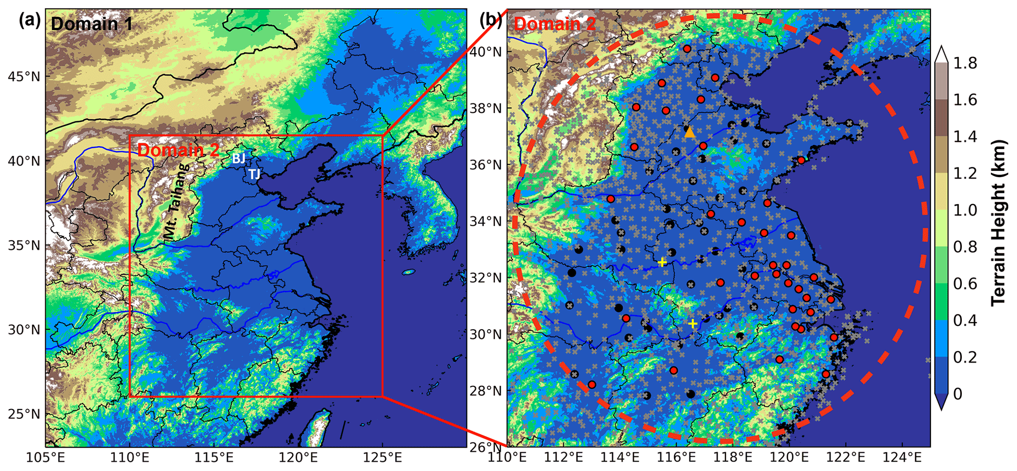
Figure 1 (a) Map of terrain height in the two nested model domains. (b) The locations of surface meteorological stations, air quality monitoring stations and sounding stations are marked by the gray crosses, red (black) dots and yellow pluses, respectively. The turbulence data site is denoted by the orange triangle. The dashed red circle indicates the areas of our primary concern.

Moreover, PBL height (PBLH) directly determines the effective air volume of pollutant diffusion and atmospheric environmental capacity. With the continuous development of technology, there are numerous means (e.g., radiosonde, tethered balloon, meteorological tower, aircraft, ground-based remote sensing and space-based remote sensing) and methods (e.g., based on surface fluxes, Richardson number and others diagnostic methods) to determine the PBLH. Of course, the results are also different (Zhang et al., 2020). It is worth noting that the PBLH is not necessarily negatively correlated with pollutant concentration (Miao et al., 2021). In particular, the turbulence barrier effect (i.e., which means turbulence may disappear at certain heights where it forms a laminar flow as if there is a barrier layer hindering the transmission up and down during the heavy pollution episodes) can impose an effect on the vertical distribution of pollutants (Ren et al., 2021), making the relationship between pollutants and the PBLH more uncertain. The PBLH can also be diagnosed by the boundary layer parameterization schemes in the model, but the PBLH does not directly determine the effective diffusion of pollutants (Jia and Zhang, 2020). Instead, vertical diffusion and mixing of pollutants are directly controlled by the turbulent diffusion coefficient (TDC), and the diagnosis of the PBLH may affect the calculation of the TDC. Previous studies have analyzed a number of pollution cases with process analysis methods (Gao et al., 2018; Chen et al., 2019). The results showed that, for a pollution event, emissions and turbulent diffusion have the greatest contribution to pollutant concentration. The evolution of pollutants is mainly controlled by turbulent diffusion, when emissions remain unchanged for a short period. Meanwhile, the contributions of dry deposition, advection transport and chemistry cannot be ignored. Consequently, more realistic turbulent diffusion characteristics are extremely important for the simulation of pollutant concentration in the model.

To date, plenty of issues remain to be addressed in the model; in particular, turbulent diffusion processes of all scalars (including active and passive scalars) are dealt with in a unified manner in the mesoscale model. Only a few studies have proposed that the meteorological fields and pollutants can be changed by adjusting the minimum value of the TDC (Savijärvi and Kauhanen, 2002; Wang et al., 2018; Du et al., 2020), increasing turbulent kinetic energy (TKE) (Foreman and Emeis, 2012) and modifying experiment expressions (Sušelj and Sood, 2010; Huang and Peng, 2017). Recently, Jia et al. (2021a) obtained the TDC of particles using high-resolution vertical flux data of particles according to the mixing length theory. Additionally, this TDC has been embedded in the Weather Research and Forecasting model coupled with Chemistry (WRF-Chem) to calculate the PBL mixing process of pollutants separately. This work has initially improved the overestimation of pollutant concentration at night in winter 2016 in eastern China. However, a series of heavy pollution incidents have occurred and attracted much attention since 2013. Therefore, we conducted a series of simulations for the heavy pollution periods in winter from 2013 to 2017 in this study. The difference between this study and previous work is that previous work focused on the observational analysis, while this study mainly explores the influence of turbulent diffusion on pollutant concentration in the mesoscale model.

2 Data and methods

2.1 Data

In this study, the aerosol pollution level is denoted by the hourly surface PM_2.5 concentration that is available from the official website of the China National Environmental Monitoring Center from 1 January 2013 to 31 January 2017. PM_2.5 concentration stations increased from 35 cities in 2013 (illustrated by red dots in Fig. 1b) to 78 cities in 2017 (illustrated by black dots in Fig. 1b) in eastern China. Except for PM_2.5 observations, the hourly concentrations of CO were acquired from the National Air Quality real-time publication platform (https://quotsoft.net/air/, last access: 5 November 2021). Meanwhile, hourly meteorological observation data (a total of 401 stations), including temperature, pressure, relative humidity, wind and visibility, from the national automatic weather stations (AWSs) are provided by the National Meteorological Information Center of China Meteorological Administration (NMICMA) (illustrated by gray crosses in Fig. 1b). The time period of the data selected is from 1 January 2013 to 31 January 2017. In addition, the turbulent diffusion of particles is calculated based on the high-frequency turbulence data, and the observational turbulence data are obtained from the Pingyuan County Meteorological Bureau (37.15^∘ N, 116.47^∘ E), Shandong Province, China, from 27 December 2018 to 8 January 2019 (illustrated by orange triangle in Fig. 1b). The experiment station is in the southern suburbs of the city of Dezhou, and there is flat farmland around this station (Figs. S1 and 2 in Ren et al., 2020). Identical eddy-covariance systems were operated, including a three-dimensional sonic anemometer–thermometer (IRGASON, Campbell Scientific, USA) and a ${\mathrm{CO}}_{\mathrm{2}}/{\mathrm{H}}_{\mathrm{2}}\mathrm{O}$ open-path gas analyzer (LI7500, LI-COR, USA). These instruments measured three components of wind speed, potential temperature, water vapor and CO₂ concentrations with a frequency of 10 Hz. The turbulence data finally were split into 30 min segments. A continuous particle measuring instrument E-sampler (Met One) and a high-frequency sampling visibility sensor (CS120A, Campbell Scientific, USA) were used to obtain PM_2.5 mass concentration every minute with a visibility of 1 Hz. The calculation of 30 min vertical flux of PM_2.5 is based on the nonlinear relationship between PM_2.5 concentration and visibility (Ren et al., 2020). The PM_2.5 concentration, temperature and wind speed at approximately 60 and 10 m were used to compute the vertical gradient of each variable. Because of the interference with the early time of the GPS sounding balloons taking off, the PM_2.5 concentration near the ground would be uncertain. Thus, we selected 10 m as the lower height to avoid that. Based on the constant flux layer hypothesis, the upper level should be within the surface layer. To facilitate the calculation, we rounded the height difference to 50 m. Finally, 60 m was selected to be the higher level to compute the vertical gradient of each variable.

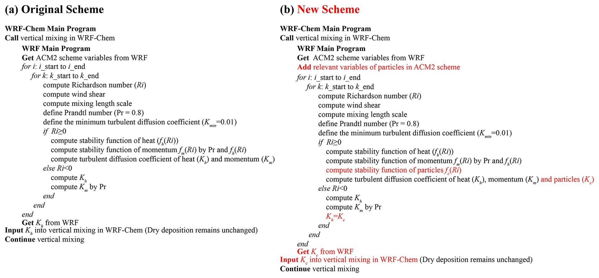
Figure 2 Flow chart of main program for turbulent diffusion coefficient in the (a) original scheme and (b) new scheme.

A detailed background and the calculation principles of this method were presented in Ren et al. (2020), so we only describe key steps here. Firstly, we separate PM_2.5 concentration (c) and visibility datasets (V) into mean and turbulent deviations (i.e., $c=\stackrel{\mathrm{‾}}{c}+c^{\prime }$ and $V=\stackrel{\mathrm{‾}}{V}+V^{\prime }$ ). Secondly, we obtain the fitted coefficients using exponential correlation (i.e., a and b) between the PM_2.5 concentration and visibility (i.e., $c=a\cdot V^b)$. Thirdly, combining the first two steps, we can obtain the turbulent fluctuations of PM_2.5 concentration (i.e., $c^{\prime }=a\cdot {\left(\stackrel{\mathrm{‾}}{V}+V^{\prime }\right)}^b-\stackrel{\mathrm{‾}}{c})$. Finally, we use fluctuations of vertical velocity (i.e., w^′) and of PM_2.5 concentration (i.e., c^′) to calculate the vertical flux of PM_2.5 (i.e., $\stackrel{\mathrm{‾}}{w^{\prime }{c}^{\prime }}$). The observed particle flux is used to calculate the Richardson function of particles later.

To illustrate the influence of the PBL height (PBLH) on the PM_2.5 pollution, soundings collected at the Fuyang site (32.54^∘ N, 115.5^∘ E) and the Anqing site (30.37^∘ N, 116.58^∘ E) (illustrated by yellow pluses in Fig. 1b) for the period 2013–2017 were analyzed. These two stations are equipped with L-band radiosonde systems (Jia et al., 2021b), which provide fine-resolution (1 Hz, and the rise rate is ∼ 6 m s⁻¹) profiles of temperature, relative humidity and wind speed two times (08:00 and 20:00 BJT) a day during winter. The Richardson number method is used to calculate the PBLH (Miao et al., 2018). The height at which the Richardson number equals 0.25 is defined as the PBLH, which is consistent with the definition of simulation.

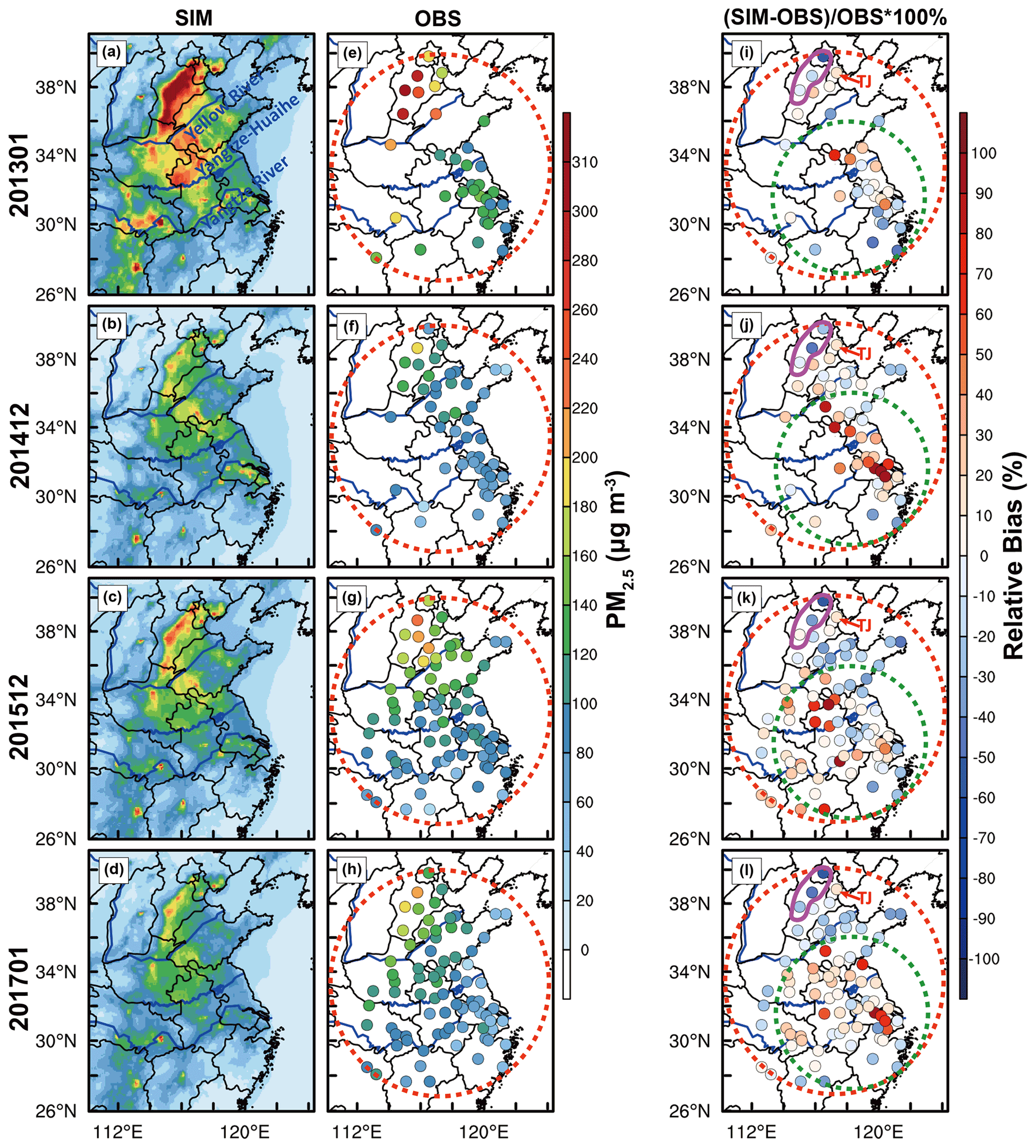
Figure 3 The average value of (a–d) simulated and (e–h) observed PM_2.5 concentration (µg m⁻³) at night and (i–l) the relative bias (RB, %) between simulation and observation. The calculation formula of relative bias is RB = $\left({\stackrel{\mathrm{‾}}{X}}_{\text{sim}}-{\stackrel{\mathrm{‾}}{X}}_{\text{obs}}\right)/{\stackrel{\mathrm{‾}}{X}}_{\text{obs}}\times \mathrm{100}$ %, where ${\stackrel{\mathrm{‾}}{X}}_{\mathrm{sim}}$ and ${\stackrel{\mathrm{‾}}{X}}_{\mathrm{obs}}$ represent the average value of simulation and observation, respectively. The locations of three rivers (i.e., Yellow River, Yangtze–Huaihe and Yangtze River) are marked by blue lines. The dashed red and green circles represent the whole simulation area and eastern China, respectively. The solid purple irregular circle indicates mountainous areas, and “TJ” in red indicates Tianjin.

2.2 Numerical simulation

Long-term three-dimensional simulation experiments are conducted using the Weather Research and Forecasting model coupled with Chemistry (WRF-Chem version 3.9.1) (Grell et al., 2005) in this study from the winter of 2013 to 2017, when eastern China frequently experienced severe and persistent aerosol pollution events. For each winter from 2013 to 2017, 1 month is selected, and a total of 4 months are confirmed, which are January 2013, December 2014, December 2015 and January 2017, respectively. The anthropogenic emissions of BC, OC, CO, NH₃, NO_x, PM_2.5, PM₁₀ and volatile organic compounds (VOCs) are set based on the latest monthly Multi-resolution Emission Inventory for China (MEIC) from 2013 to 2017, provided by Tsinghua University, with a resolution of $\mathrm{0.25}{}^{\circ }\times \mathrm{0.25}{}^{\circ }$ (http://meicmodel.org/, last access: 20 May 2021). The model domain was centered over eastern China with a horizontal resolution of 33 and 6.6 km (Fig. 1a). The model top was set to the 50 hPa level, and 48 vertical layers were configured below the top. To resolve the PBL structure, 21 vertical layers were set below 2 km (i.e., the specific setting of vertical levels is σ=1.000, 0.997, 0.994, 0.991, 0.988, 0.985, 0.980, 0.975, 0.970, 0.960, 0.950, 0.940, 0.930, 0.920, 0.910, 0.895, 0.880, 0.865, 0.850, 0.825, 0.800). The physics parameterization schemes selected for this study included the Morrison double-moment microphysics scheme (Morrison et al., 2009), RRTMG longwave/shortwave radiation schemes (Iacono et al., 2008), the MM5 similarity surface layer scheme (Jiménez et al., 2012), the Noah land surface scheme (Chen and Dudhia, 2001), the single-layer UCM scheme (Kusaka et al., 2001), the CLM4.5 lake physics scheme (Gu et al., 2015), the ACM2 planetary boundary layer scheme (Pleim, 2007) and the Grell-3D cumulus scheme (Grell and Devenyi, 2002). And the chemical mechanism is the RADM2-MADE/SORGM scheme (Ackermann et al., 1998; Schell et al., 2001). The initial and boundary conditions of meteorological fields were set up using the National Centers for Environmental Prediction (NCEP) global final (FNL) reanalysis data, with a resolution of $\mathrm{1}{}^{\circ }\times \mathrm{1}{}^{\circ }$ (https://rda.ucar.edu/datasets/ds083.2/, last access: 20 May 2021). And the initial and boundary conditions of chemical fields were configured using the global model output of the Model for Ozone and Related Chemical Tracers (MOZART) (http://www/acom.ucar.edu/wrf-chem/mozart.shtml, last access: 20 May 2021).

Figure 2 shows the flow chart of the main program related to the turbulent diffusion coefficient. Simulations using the abovementioned configurations are referred to as the original runs. In the original PBL parameterization scheme, TDCs of heat and momentum are different (i.e., K_h≠K_m). The turbulent mixing process of pollutants is considered to be similar to that of heat, which supposes the turbulent diffusion of particles and heat is identical (i.e., K_h=K_c) (Fig. 2a), while in the new scheme, the turbulent mixing process of pollutants is calculated by the TDC of particles (i.e., K_c), which is different from the TDC of heat (i.e., K_h≠K_c). These improved experiments are regarded as the new runs hereafter (Fig. 2b). All simulations included a total of 8 months. The 91 h simulation is conducted beginning from 00:00 UTC of 3 d ago for each day (i.e., 248 simulation experiments), the first 64 h of each simulation is considered as the spin-up period, the next 24 h is used for further analysis and the remaining 3 h is discarded (e.g., run one simulation from 00:00 UTC (08:00 BJT) on 29 December to 18:00 UTC (12 January, 02:00 BJT) on 1 January and 91 h in total. We need the results from 00:00 to 23:00 BJT on 1 January. The period from 08:00 BJT on 29 December to 23:00 BJT on 31 December is considered as the spin-up period (in total 64 h), and the results from 00:00 to 02:00 BJT on 2 January are discarded).

Figure 4 The average value of (a–d) simulated PM_2.5 concentration (µg m⁻³) by new schemes, (e–h) the relative bias (RB, %) of PM_2.5 concentration between simulation of new scheme and observation and (i–l) the absolute bias (AB, %) between the new and original schemes. The calculation formula of absolute bias is $\mathrm{AB}=\left|{\mathrm{RB}}_{\mathrm{new}}\right|-\left|{\mathrm{RB}}_{\mathrm{original}}\right|$ , where |RB_new| and |RB_original| represent the relative bias of new and original schemes, respectively. The dashed red and green circles represent the whole simulation area and eastern China, respectively.

2.3 Calculation principle of turbulent diffusion of particles

Considering that the pollution is usually accompanied by the stable boundary layer (SBL), and the simulation results of pollutant concentration are poor in the SBL at night, we mainly modify the program of the stable boundary layer, while for the unstable boundary layer, we still use the default program of the original scheme (Fig. 2). Although the turbulent vertical mixing and dry deposition are calculated in the same program in WRF-Chem, we only modified the turbulent diffusion in the new scheme. Here, we briefly describe the information about dry deposition. We adopt the MADE/SORGAM aerosol scheme, in which the dry deposition is calculated based on Binkowski's method (Binkowski and Shankar, 1995). The dry deposition velocity (V_d) can be expressed as $V_{\text{d}}=V_{\text{g}}+\mathrm{1}/\left(R_{\text{a}}+R_{\text{s}}+R_{\text{a}}\cdot R_{\text{s}}\cdot V_{\text{g}}\right)$, where V_g is the gravitational settling velocity, R_a is the aerodynamic resistance and R_s is the canopy resistance.

The TDC is parameterized by the mixing length (l) and the function of Richardson number (f(Ri)) based on mixing length theory; that is

$$\begin{array}{}\text{(1)}& K=\mathrm{0.01}+\sqrt{\mathrm{ss}\cdot }{l}^{\mathrm{2}}\cdot f\left(Ri\right),\end{array}$$

where ss is the wind shear (i.e., ss = ${\left(\partial \stackrel{\mathrm{‾}}{u}/\partial z\right)}^{\mathrm{2}}+{\left(\partial \stackrel{\mathrm{‾}}{v}/\partial z\right)}^{\mathrm{2}})$, and 0.01 refers to the minimum value of the TDC in the model. The minimum value of the TDC remains unchanged in the new scheme. The mixing length formula (i.e., $l=kz/(\mathrm{1}+kz/\mathit{\lambda })$, λ=80) is proposed by Blackadar (1962), and it is widely used in the model. Ri is the gradient Richardson number (i.e., $Ri=\left(g/\stackrel{\mathrm{‾}}{{\mathit{\theta }}_v}\right)\partial \stackrel{\mathrm{‾}}{{\mathit{\theta }}_v}/\partial z\left[(\partial \stackrel{\mathrm{‾}}{u}/\partial z{)}^{\mathrm{2}}+{\left(\partial \stackrel{\mathrm{‾}}{v}/\partial z\right)}^{\mathrm{2}}\right]$), where z is the observation height, g is the gravity, θ_v is the virtual potential temperature, and u and v are the component of wind), which is approximated in finite difference form, and the resulting parameter is sometimes referred to as the bulk Richardson number (Garratt, 1992). For example, Louis et al. (1982) suggest that Ri is the bulk Richardson number, but the expression is in the form of the gradient Richardson number (Eq. 5 in Louis et al., 1982). Many previous studies have shown various functions of the Richardson number, which represent the different situations of turbulence. Here, we mainly compare the similarities and differences between the turbulent diffusion of momentum, heat and particles in the model.

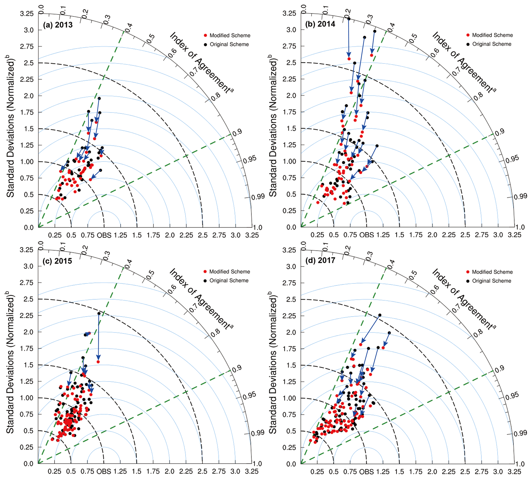
Figure 5 Taylor diagram of simulation by original scheme and modified scheme. XY axes and arcs represent the normalized standard deviations (NSDs; $\mathrm{NSD}=\frac{\sqrt{\frac{\mathrm{1}}{N-\mathrm{1}}\sum _{i=\mathrm{1}}^n{\left(X_{\text{sim},i}-{\stackrel{\mathrm{‾}}{X}}_{\text{sim}}\right)}^{\mathrm{2}}}}{\sqrt{\frac{\mathrm{1}}{N-\mathrm{1}}\sum _{i=\mathrm{1}}^n{\left(X_{\text{obs},i}-{\stackrel{\mathrm{‾}}{X}}_{\text{obs}}\right)}^{\mathrm{2}}}}$, where ${\stackrel{\mathrm{‾}}{X}}_{\text{sim}}$ and ${\stackrel{\mathrm{‾}}{X}}_{\text{obs}}$ represent the average value of simulation and observation, respectively) and index of agreement (IOA, $\mathrm{IOA}=\mathrm{1}-\frac{\left[\sum _{i=\mathrm{1}}^n{\left|X_{\text{sim},i}-X_{\text{obs},i}\right|}^{\mathbf{2}}\right]}{\left[\sum _{i=\mathrm{1}}^n{\left(\left|X_{\text{sim},i}-{\stackrel{\mathrm{‾}}{X}}_{\text{obs}}\right|+\left|X_{\text{obs},i}-{\stackrel{\mathrm{‾}}{X}}_{\text{obs}}\right|\right)}^{\mathrm{2}}\right]}$, where X_sim,i and X_obs,i represent the value of simulated and observed, respectively; i refers to time, and n is the total number of time series), respectively. All cities (a total of 35 cities in 2013 and 78 cities in 2014, 2015 and 2017) are shown by dots, and black (red) represents the original (new) scheme. The root mean square (rms) is denoted by the dashed blue line, and the arrow indicates the change of the new scheme compared to the original scheme at the same station.

For the stable conditions (i.e., Ri≥0), Esau and Byrkjedal (2007) suggested

$$\begin{array}{}\text{(2)}& {\displaystyle }{f}_{\text{h}}={\left(\mathrm{1}+\mathrm{10}Ri+\mathrm{50}R{i}^{\mathrm{2}}+\mathrm{5000}R{i}^{\mathrm{4}}\right)}^{-\mathrm{1}}+\mathrm{0.0012},\text{(3)}& {\displaystyle }{f}_{\text{m}}=\mathrm{0.8}{f}_{\text{h}}+\mathrm{0.00104},\end{array}$$

where f_h and f_m denote the functions of heat and momentum, respectively, and these functions existed in the original model. We added an additional function of particles into the model; that is

$$\begin{array}{}\text{(4)}& f_{\text{c}}={\left(\mathrm{1}+\mathrm{66.6}Ri\right)}^{-\mathrm{1}},\end{array}$$

which is used to denote the turbulent mixing process of particles within the PBL. When Ri is greater than ∼ 0.2, the TDC of particles is greater than that of heat, which may reduce pollutant concentration. With the increase of instability, the TDC of particles is gradually smaller than that of heat, theoretically leading to the increase of pollutant concentration. For detailed analysis and comparison of functions, please refer to Jia et al. (2021a).

For the unstable conditions (Ri<0),

$$\begin{array}{}\text{(5)}& {\displaystyle }{f}_{\text{h}}=f_{\text{c}}={\left(\mathrm{1}-\mathrm{25}Ri\right)}^{\mathrm{1}/\mathrm{2}},\text{(6)}& {\displaystyle }{f}_{\text{m}}=Pr\cdot f_{\text{h}},\end{array}$$

where the TDC of particles is still equal to that of heat (i.e., K_c=K_h), while the TDC of momentum is calculated by the turbulent Prandtl number (i.e., Pr, Pr=0.8).

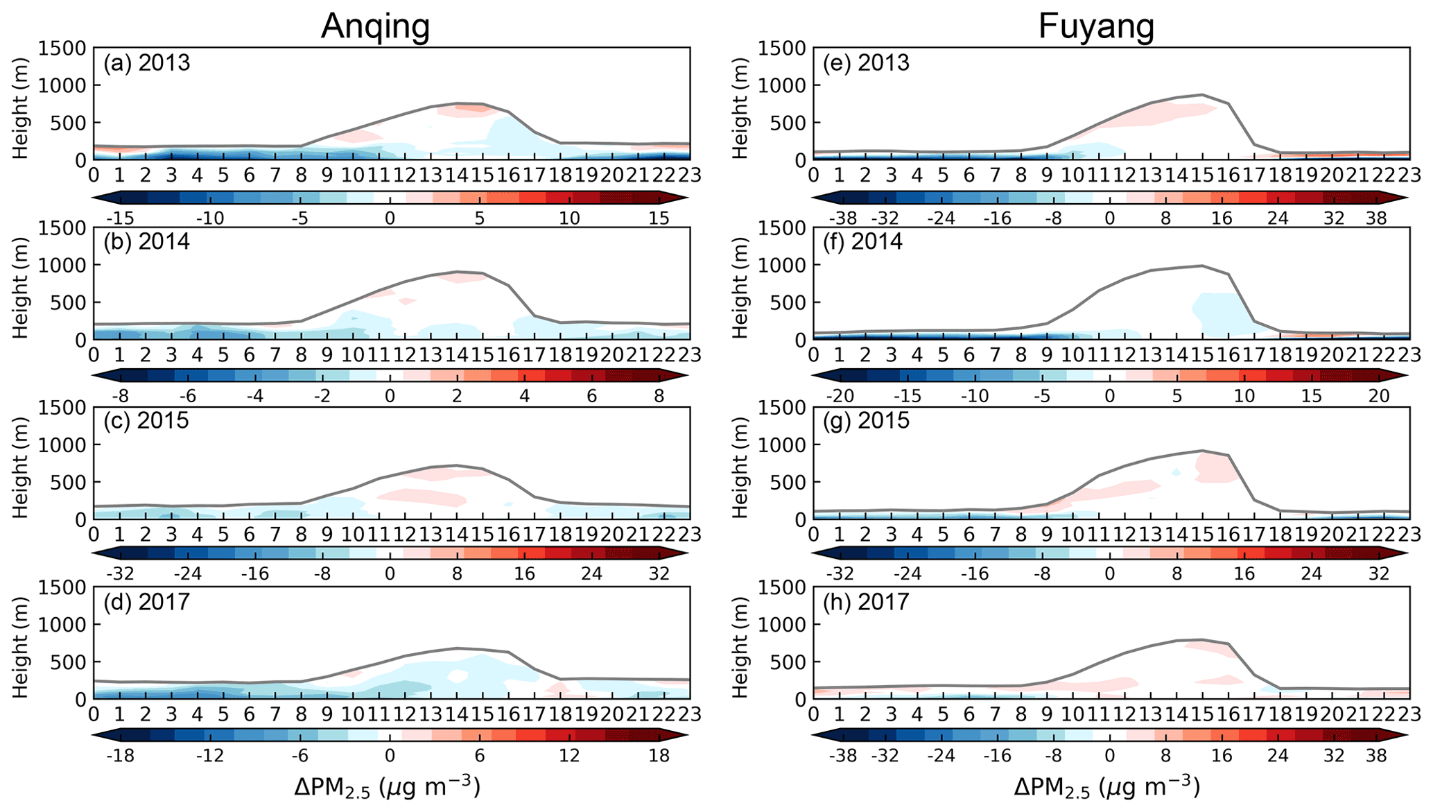
Figure 6 Time–height cross sections for the difference of PM_2.5 concentration between original and new schemes (i.e., the new scheme minus the original scheme) within the PBL in (a–d) Anqing and (e–h) Fuyang from 2013 to 2017. The gray line indicates the PBLH.

There is much important information about the TDC of particles that needs to be illustrated. (1) Turbulent diffusion of particles calculated by the explicit local gradient represents the PBL mixing process of particles, which is more suitable in the stable boundary layer (SBL) (Mahrt and Vickers, 2003). (2) The uncertainty of turbulent diffusion coefficient calculated by the PBLH and the Monin–Obukhov similarity theory (MOST) at night is large, which has been avoided in the new scheme. Meanwhile, the computational efficiency based on mixing length is higher (Li et al., 2010), and it is easier to apply to forecasting models in the future. (3) Turbulent diffusion of particles is used to evaluate the PBL mixing process of pollutants separately, which can affect the simulation results of pollutants and not influence the simulation results of meteorological parameters.

Figure 7 Time series of the observed (black) and simulated (red) PBLH at 08:00 and 20:00 (BJT) in (a–d) Anqing and (e–h) Fuyang from 2013 to 2017.

3 Evaluation of PM_2.5 concentration simulation

Based on the TDC relationship of particles in the previous study (Jia et al., 2021a), this study applies this relationship to a long-term scale simulation for verification. Figure 3 shows the average value of simulated and observed PM_2.5 concentration at night (i.e., from 18:00 on the first day to 07:00 on the second day) from 2013 to 2017, and the simulation results can better reproduce the distribution of pollutant concentration (i.e., represented by the dashed red circle). However, the PM_2.5 concentration was overestimated to varying degrees in eastern China (i.e., indicated by the dashed green circle), and the mean value of relative bias (RB) of the region is as high as 11.8 % (2013), 48 % (2014), 23.8 % (2015) and 20.9 % (2017), respectively (Fig. 3i–l). In addition, we also found that the pollutant concentrations are underestimated in Beijing (BJ) and along the Taihang Mountains (Mt. Taihang) (i.e., indicated by the purple irregular circle) but overestimated in Tianjin (TJ) (Fig. 3i–l). Why is the pollutant concentration simulated by the same model different in each region? What are the different effects of turbulent diffusion in different regions? These issues will be further explained later, and this section primarily evaluates the simulation results of the pollutant concentration. Compared to the original scheme, the new scheme improves the situation where the pollutant concentration is overestimated at night in eastern China (Fig. 4a–d). The degree of overestimation of the pollutant concentration is reduced, and the mean value of relative bias of the new scheme is 3.5 % (2013), 31 % (2014), 12.8 % (2015) and 9.2 % (2017), respectively (Fig. 4e–h). In addition, the mean value of the absolute bias is decreased by 8.3 % (2013), 17 % (2014), 11 % (2015) and 11.7 % (2017), respectively (Fig. 4i–l). In summary, compared with the original scheme, the new scheme can generally improve the overestimation of pollutant concentration in eastern China, due to the changes in turbulent diffusion. For the above stations where the pollutant concentration was underestimated in the original scheme, the pollutant concentration will be further underestimated with the increase in turbulent diffusion. However, this underestimation cannot be avoided because there is an opposite phenomenon in the pollutant concentration in the two regions. We can only look at the differences in the two regions from other perspectives (see Sect. 4 for details), as the model is fraught with uncertainties.

Figure 8 The relative bias (%) between simulation and observation at all environment monitoring stations and terrain height in Beijing–Tianjin–Hebei in (a) 2013, (b) 2014, (c) 2015 and (d) 2017. Taihang Mountain (Mt. Taihang) and Yan Shan (Mt. Yan) are indicated by the red text, Beijing (BJ), Tianjin (TJ) and Hebei (HB) are represented by purple abbreviations and the dividing line between overestimated and underestimated areas is indicated by a dashed white line.

To better evaluate the model performance, Fig. 5 shows the Taylor diagram of hourly PM_2.5 concentration, and the black (red) dots indicate original (new) simulation results at all stations from 2013 to 2017. The statistical results have a consistent feature; that is, the worse the simulation results of the original scheme are, the more obvious the improvement of the new scheme becomes (arrows indicate improved stations in the Fig. 5). The results indicate that the pollutant concentrations are not improved to the same degree at all stations. When the simulation of pollutant concentration is overestimated in the original scheme, the new scheme improves the degree of overestimation. While the simulation of pollutant concentration is underestimated in the original scheme, the new scheme cannot further underestimate, and the degree of “re-underestimate” is not obvious (Figs. 5 and S2). And the mean value of standard deviation (normalized) is decreased by 0.2 (2013), 0.28 (2014), 0.14 (2015) and 0.16 (2017) (Fig. 5). As a whole, the new scheme can improve the common phenomenon of overestimated pollutant concentration at night in eastern China (Fig. 5).

As turbulent diffusion increases, the pollutant concentration gradually decreases. Where do the reduced pollutants go? Do they spread to the surrounding area in the horizontal direction or diffuse to the upper level in the vertical direction? This question warrants a more in-depth discussion. It can be seen from Fig. 4 that the reduction in pollutant concentration is a regional synchronous change, and there is no regular concentration gradient in the horizontal direction. Therefore, we should also pay more attention to the changes in the vertical direction. Theoretically, increasing turbulent diffusion can reduce the pollutant concentrations near the surface layer, and the pollutants can be more fully mixed in the vertical direction, leading to lower pollutant concentration in the near-surface layer and higher in the upper layer. As we expect, the pollutant concentration is reduced in the surface layer and increased in the upper layer at night in eastern China (Figs. 6, S3–S5), which is consistent with the theory.

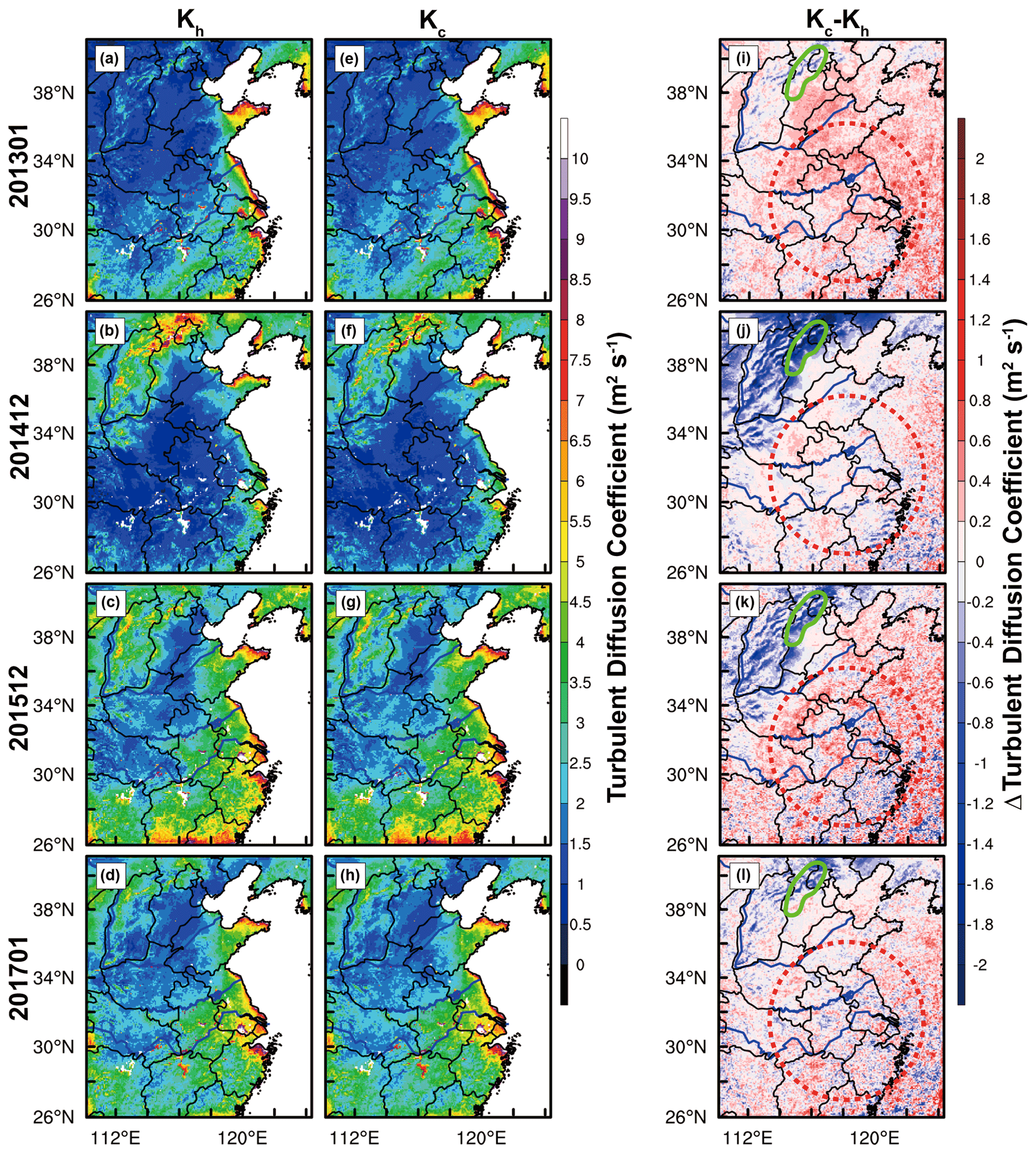
Figure 9 Turbulent diffusion coefficient of (a–d) heat and (e–h) particles and (i–l) the difference between two turbulent diffusion coefficients. The dashed red and solid green irregular circles represent eastern China and mountainous areas, respectively.

4 Uncertainty analysis

4.1 Meteorological parameters

Depending on the high-frequency particle flux, the TDC of particles has been added into the model to compute the turbulent mixing process of particles separately. Compared with previous studies about the improvement of parameterization scheme, the greatest strengths of the new scheme are that it not only improves the simulation results of pollutant concentration, but also does not deteriorate the simulation results of other parameters. To verify that the new scheme does not affect the simulation results of the meteorological parameters, the simulation results of the near-surface meteorological elements (i.e., 2 m temperature, 2 m relative humidity and 10 m wind speed) between the original and new schemes have been compared and analyzed. It can be seen from Figs. S6–S8 that the correlation coefficients of meteorological parameters by the two schemes are greater than 0.99. Noting that the new scheme does not alter the performance of meteorological fields, it is an advantage of the new scheme. As mentioned earlier, modifying the turbulent diffusion coefficient of heat not only affects the simulation of temperature (Savijärvi and Kauhanen, 2002), but also affects the results of pollutants (Du et al., 2020).

Improving the parameterization scheme is a long and tough process, making it difficult to improve the simulation results of all parameters at the same time. When the simulation results of one parameter are improved, we should first ensure that the simulation results of other parameters are not deteriorated. Then, we will work on improving other parameters. Although the aerosol–radiation two-way feedback process is considered in the WRF-Chem model, the change in PM_2.5 concentration caused by radiation feedback is only by a few percent (Li et al., 2017; Wu et al., 2019). We should focus more on the impact of turbulence on aerosol pollution, and we need to pay more attention to some turbulent characteristics (e.g., turbulence barrier effect and turbulent intermittency) during heavy pollution episodes (HPEs), which can reflect a more realistic evolution process of pollutant concentration. We will further clarify the relationship between particles, momentum and heat transport through observational data, so as to lay the foundation for model improvement.

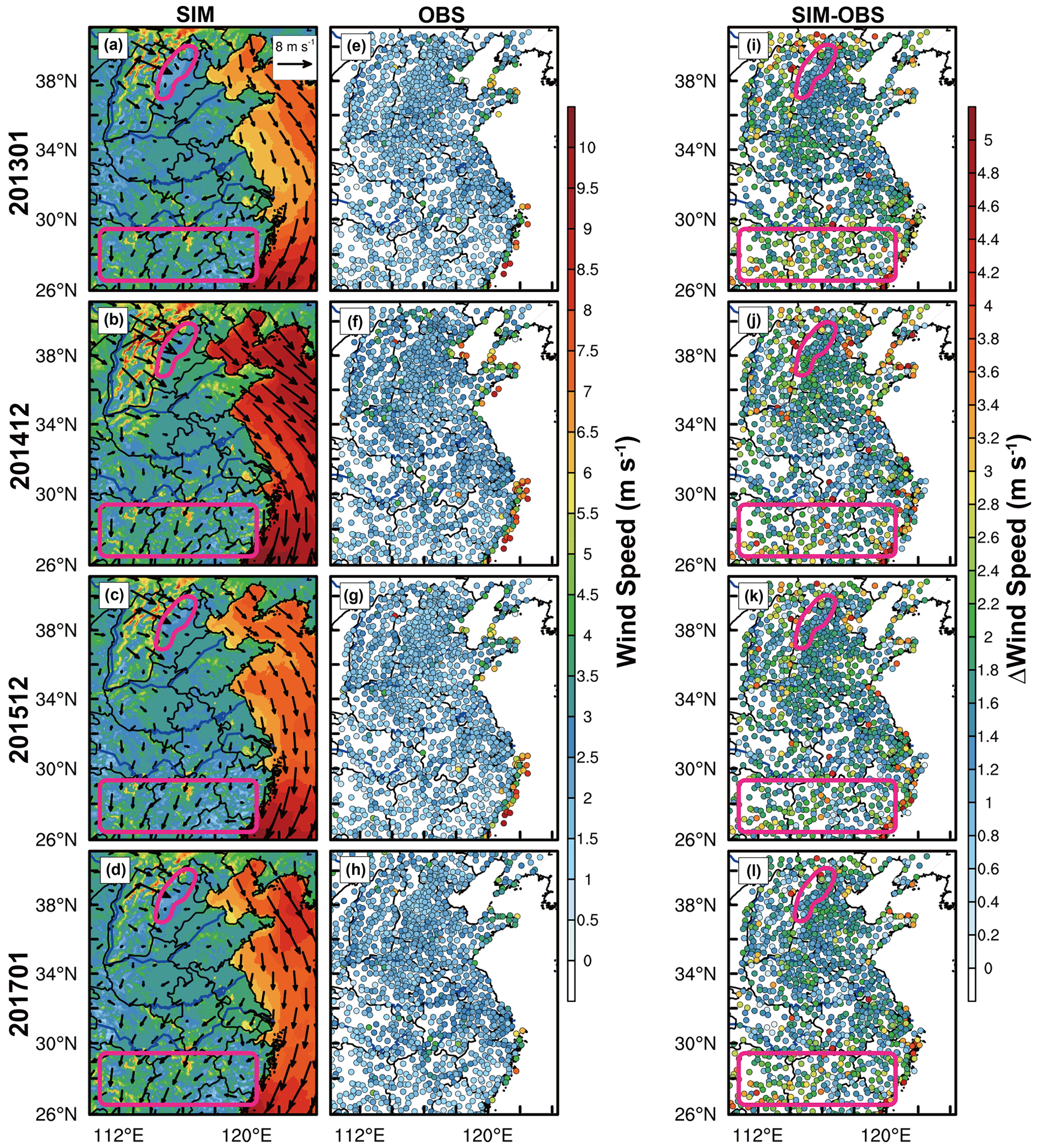
Figure 10 (a–d) Simulated and (e–h) observed wind speed at 10 m a.g.l. and (i–l) the difference between simulated and observed wind speed. The purple rectangle indicates the area where the observed wind speed is significantly overestimated.

4.2 PBL height

Although the PBL height (PBLH) is widely used to determine the effective air volume and atmospheric environmental capacity for pollutant diffusion, various methods diagnose different PBLHs, which reinforces uncertainty about the PBLH as a criterion. When there is a transport stage with a high wind speed during HPEs, the mechanical turbulence is strong, and the pollutant concentration and PBLH increase simultaneously (Jia et al., 2021b; Miao et al., 2021). As a result, the relationship between PBLH and PM_2.5 pollution is intricate. The impact of the PBLH is ultimately represented through the TDC in the model, as the PBLH is used to calculate the TDC (Jia et al., 2021a). And artificially changing the PBLH can also affect the simulation of pollutant concentration. If the simulation error in pollutant concentration is caused by the PBLH, then the pollutant concentration is overestimated, and the PBLH should be underestimated. However, the PBLH is well reproduced by the model, while the model does not underestimate PBLH (Fig. 7). Anqing is located in the mountain corridor, where the simulation results of PBLH (index of agreement, IOA = 0.49–0.81) are slightly worse than in Fuyang (IOA = 0.63–0.85). That is to say, various factors can influence the calculation of PBLH.

A more accurate PBLH can reduce some uncertainty in the model, but how to apply the accurate PBLH through observation to the model is a thorny problem. For example, the turbulence barrier effect modifies the mixing height of pollutants (Ren et al., 2021), which cannot be reflected in the model, and it can lead to deviation in the simulation of pollutant concentration. The new scheme does not disturb the simulation results of meteorological fields and, thus, does not affect the simulation results of PBLH (Fig. S9). The simulation results of pollutant concentrations are improved under a similar PBLH, further demonstrating that the simulation of pollutant concentration is not only controlled by the PBLH, but also influenced by turbulent diffusion. Finally, turbulent diffusion controls the mixing of pollutant concentration and the evolution of meteorological parameters.

4.3 Influence of other processes

Overestimation of pollutant concentrations has been improved in eastern China, but there are also some stations in northern China where pollutant concentrations are underestimated (Fig. 3i–l). Therefore, the stratification is more stable in most of the nighttime in eastern China (Ri is greater than ∼ 0.2, based on the fitting function in Jia et al., 2021a), while the stratification tends to be weakly stable/unstable at the same time in the mountainous area with complex terrain. These stations (i.e., Hebei and Beijing) are mostly located in the east of the Taihang Mountains and the south of the Yan Mountains (Fig. 8). For example, in December 2016, the pollutant concentrations of all stations in Beijing were not underestimated. Jia et al. (2021a) found that the pollutant concentrations of two stations located in the south of Beijing (i.e., blue dots in Fig. S2 in Jia et al., 2021a) are well reproduced by the model. This phenomenon of pollutant concentrations being significantly underestimated at some stations near the mountainous area also occurred in 2013–2017 (Fig. 8). The boundaries of overestimated and underestimated sites are pronounced in the Beijing–Tianjin–Hebei region (dashed white line in Fig. 8), and the pollutant concentration is overestimated at some stations away from the mountainous area (i.e., Tianjin and southeast of Hebei). Meanwhile, the TDC of particles in the new scheme is greater than that of heat in the original scheme in eastern China (i.e., dashed red circle in Fig. 9i–l); that is, the increased turbulent diffusion improves the overestimation of pollutant concentration in this area. Compared to the original scheme, the increase in the TDC in the new scheme is attributed to the change in f(Ri) when other physical quantities remain unchanged. What is more, we find that the TDC in the new scheme is much smaller than that in the original scheme in the mountainous area (i.e., green irregular circle in Fig. 9). Theoretically, the reduced TDC is expected to increase the pollutant concentration and improve the underestimation of pollutant concentration in the original scheme. Disappointingly, the change in the TDC does not improve the underestimation of pollutant concentration in the mountainous area (Figs. 8, 9i–l), indicating that the change in turbulent diffusion is not sensitive to the pollutant concentration in the mountainous area.

In addition to the main influencing factors of emission and turbulent diffusion, advection transport, chemistry processes and dry deposition can also affect the simulation of pollutant concentration. Given that we are using the latest emissions source inventory, it is impossible to use other more elaborate inventories to quantify the uncertainty caused by emissions. The advection process is strongly related to wind and PM_2.5 concentration gradients from upwind areas to downwind areas (Gao et al., 2018). Figure 10 shows the simulation results of wind speed, and we find that the wind speed is overestimated in the whole simulation area. The model often overestimates the wind speed, which is the reason for the model itself (Jia and Zhang, 2020). Nevertheless, there are regional differences in the overestimation of wind speed, which is more obvious in areas with complex terrain (framed by purple lines in Fig. 10). Jiménez and Dudhia (2012) indicated that the overestimation of wind speed may be caused by the incorrect description of sub-grid surface roughness. For the purple rectangle region, although the wind speed is overestimated, there is no evident wind speed gradient and pollutant concentration gradient (Figs. 3a–d, 10a–d). Thus, the effect of advection is insignificant, while for the irregular purple region, we can see that the wind speed gradient and pollutant concentration gradient are obvious (Figs. 3a–d, 10a–d). In the northwest of the irregular purple area, clean air will pass through this area under the control of stronger northwesterly wind. Consequently, this area is extremely susceptible to advection transport; therefore, the pollutant concentration has been underestimated here. We should pay more attention to the improvement of wind field simulation in complex terrain. It is expected that the simulation of the wind field will be improved, leading to an improvement in pollutant concentration in this area.

The chemistry process, i.e., the PM_2.5 concentration contribution caused by secondary transformation, was negligible in this study and is not mentioned further in this paper. Whether the simulation of chemical components has been improved cannot be properly verified because of the lack of observational data. Although the simulation results of PM_2.5 components cannot be evaluated, CO, as a representative of primary pollutants, can be compared with the observations. Results from the new scheme with the TDC of particles are more consistent with the observations than the original scheme (Fig. S10), giving support to the improvement of PM_2.5 concentration (Figs. 5 and S10). Moreover, the dry deposition process of particles is also extremely important (Zhang et al., 2001; Farmer et al., 2021). The turbulent mixing and dry deposition processes belong to the same main program in the mesoscale model. However, as particle size increases, particle inertia and gravity cannot be neglected, but these inertia and gravity effects are neglected for particles smaller than 10 µm in diameter (Fratini et al., 2007). In this sense, we did not include the influence of gravity on pollutant concentration in this study. Petroff and Zhang (2010) showed that according to the method in Zhang et al. (2001), the dry deposition can be overestimated, especially for fine particles. Special attention must be paid to the fact that the overestimation of dry deposition affects the distribution of pollutant concentration. Therefore, the choice of dry deposition scheme also needs to be carefully considered, in that this process is also very important for the evolution of pollutants. In the future, long-term simulation results should be used to verify the difference in aerosol process decomposition in detail.

5 Conclusions and prospects

At present, the mesoscale model is facing numerous challenges, especially the accurate simulation of pollutant concentration during heavy pollution episodes. One of these challenges is to correctly describe the turbulent mixing process of pollutants. Though the model can reproduce the evolution of pollutants, the simulation of diurnal variation of pollutants is fundamentally flawed, especially at night. Errors in the estimation of pollutant concentration are primarily caused by defects in the turbulent mixing of pollutants in the model. Actually, a difference exists between the turbulent transport of heat and particles, which inspires us to deal with the turbulent diffusion of heat and particles separately. Therefore, based on the turbulent diffusion expression of particles proposed by Jia et al. (2021a), we demonstrate the improvement of pollutant concentration in winter from 2013 to 2017, and the uncertainty factors are also analyzed in the model.

The original scheme overestimates the surface PM_2.5 concentration by 11.8 % (2013), 48 % (2014), 23.8 % (2015) and 20.9 % (2017) at night, respectively. The new scheme has improved the overestimation of the surface PM_2.5 concentration in eastern China at night, and the mean value of absolute bias of the region can be reduced by 8.3 % (2013), 17 % (2014), 11 % (2015) and 11.7 % (2017), respectively. In the horizontal direction, the pollutant concentration shows regional synchronous changes. Consequently, the pollutant concentration is reduced near the surface layer and better mixed in the entire layer, increasing the pollutant concentration in the upper level. Moreover, the new scheme not only improves the simulation of pollutant concentration, but also does not deteriorate the simulation of other meteorological parameters. Although the PBLH affects the diffusion of pollutants, the simulation of pollutant concentration is not specifically controlled by the PBLH. It should be noted that the TDC has a negligible impact on the simulation of pollutant concentration at some stations with complex topography. Meanwhile, advection transport may dominate the evolution of pollutant concentration in mountainous area. The simulation results of PM_2.5 components cannot be evaluated, owing to the lack of observational data. CO, however, as a representative of primary pollutants, can be compared with observations. Results from the new scheme are more consistent with the observations than the original scheme, which supports the improvement of the PM_2.5 concentration.

The coefficient of function in this study should be discussed combined with the sample size of data, but we hope the new scheme can provide promising guidance during heavy pollution episodes. The turbulent transport mechanism and turbulence parameterization constitute a complex topic (Couvreux et al., 2020; Edwards et al., 2020), and beyond this, other processes (or other parameters) require in-depth understanding and exploration (Zhang et al., 2001; Shao et al., 2019; Emerson et al., 2020). Hence, more research may shed more light on the turbulent mixing process and transport mechanisms of pollutants during heavy pollution episodes, especially on the experimental side (e.g., by carrying out extensive measurement campaigns).