the Creative Commons Attribution 4.0 License.
the Creative Commons Attribution 4.0 License.
 | 05 Nov 2021
The effects of the COVID-19 lockdowns on the composition of the troposphere as seen by In-service Aircraft for a Global Observing System (IAGOS) at Frankfurt
Yasmine Bennouna
Maria Tsivlidou
Pawel Wolff
Bastien Sauvage
Brice Barret
Eric Le Flochmoën
Romain Blot
Damien Boulanger
Jean-Marc Cousin
Philippe Nédélec
Andreas Petzold
Valérie Thouret
The European research infrastructure IAGOS (In-service Aircraft for a Global Observing System) equips commercial aircraft with a system for measuring atmospheric composition. A range of essential climate variables and air quality parameters are measured throughout the flight, from take-off to landing, giving high-resolution information in the vertical in the vicinity of international airports and in the upper troposphere–lower stratosphere during the cruise phase of the flight. Six airlines are currently involved in the programme, achieving a quasi-global coverage under normal circumstances. During the COVID-19 crisis, many airlines were forced to ground their fleets due to a fall in passenger numbers and imposed travel restrictions. Deutsche Lufthansa, a partner in IAGOS since 1994 was able to operate an IAGOS-equipped aircraft during the COVID-19 lockdown, providing regular measurements of ozone and carbon monoxide at Frankfurt Airport. The data form a snapshot of an unprecedented time in the 27-year time series. In May 2020, we see a 32 % increase in ozone near the surface with respect to a recent reference period, a magnitude similar to that of the 2003 heatwave. The anomaly in May is driven by an increase in ozone at nighttime which might be linked to the reduction in NO during the COVID-19 lockdowns. The anomaly diminishes with altitude becoming a slightly negative anomaly in the free troposphere. The ozone precursor carbon monoxide shows an 11 % reduction in MAM (March–April–May) near the surface. There is only a small reduction in CO in the free troposphere due to the impact of long-range transport on the CO from emissions in regions outside Europe. This is confirmed by data from the Infrared Atmospheric Sounding Interferometer (IASI) using retrievals performed by SOftware for a Fast Retrieval of IASI Data (SOFRID), which display a clear drop of CO at 800 hPa over Europe in March but otherwise show little change to the abundance of CO in the free troposphere.
- Article
(4740 KB) - Full-text XML
- BibTeX
- EndNote


The World Health Organization declared the global COVID-19 pandemic in March 2020 (WHO, 2020). The serious threat to public health led countries to adopt lockdowns and other coordinated restrictive measures aimed at slowing the spread of the virus. Such measures had an important effect on economic activity and by consequence on the emissions of primary pollutants from industrial and transport sectors. Much discussed is the extent to which these lockdowns have had a significant effect on local air quality and more widely on atmospheric composition (e.g. Bauwens et al., 2020; Lee et al., 2020) and climate (Le Quéré et al., 2020).
Many studies have focused on primary pollutants such as NO2, decreases of which were almost immediately apparent in satellite imagery from the TROPOspheric Monitoring Instrument (TROPOMI) on the Sentinel-5 Precursor satellite (Veefkind et al., 2012) over China in January–February (Liu et al., 2020) and later over Europe (Bauwens et al., 2020). Emissions of NO2 are strongly linked to economic activity (Duncan et al., 2016). Instruments such as TROPOMI have registered weekly cycles of NO2 and drops in NO2 related to behavioural patterns of work and holiday periods (Beirle et al., 2003; Tan et al., 2009). Thus, the large reductions in NO2 in the tropospheric column during lockdown over the most economically active areas of Europe (in particular the Po Valley, Italy) were quickly associated with the drop in industrial output and emissions from transport. Reductions of between 20 % and 38 % compared with the same periods in previous years were recorded (Bauwens et al., 2020). However, TROPOMI is a young instrument, launched in October 2017, and as such, there is not a robust climatology with which to compare these changes during lockdown and in particular to control for the influence of different meteorological conditions (e.g. Goldberg et al., 2020). Relevant weather conditions might include higher planetary boundary layer heights which drive down the surface concentrations of pollutants irrespective of any changes in emissions; windy periods, with their impact on the dispersion and deposition of NO2; and cloudy skies with their impact on satellite retrievals. As TROPOMI is sensitive to clouds, using only cloud-free columns can lead to a negative sampling bias. In many parts of Europe, skies were unusually clear (van Heerwaarden et al., 2021; https://surfobs.climate.copernicus.eu/stateoftheclimate/march2020.php, last access: 3 November 2021) due to the persistence of anticyclonic conditions and strongly reduced air traffic (Schumann et al., 2021b, a), and a negative bias may have been reinforced during the lockdown period (e.g. Barré et al., 2021; Schiermeier, 2020; , last access: 3 November 2021).
Drops in primary pollutants were also evident from ground-based air quality networks across Chinese and European cities; see the review by Gkatzelis et al. (2021) for a comprehensive overview. In Spain's two largest cities, where lockdowns were extremely strict, the reductions in NO2 concentrations were 62 % and 50 % (Baldasano, 2020). Lee et al. (2020) calculated an average reduction in NO2 of 42 % across 126 sites in the UK, with a 48 % reduction at sites close to the roadside due to the drop in traffic emissions. Y. Wang et al. (2020) looked at six different pollutants (PM2.5, PM10, CO, SO2, NO2 and O3) and found large reductions in NO2 from traffic sources and a smaller reduction in CO from reduced industrial activities in northern China. Similarly, Shi and Brasseur (2020) also noted a drop in CO across the monitoring stations in northern China operated by the China National Environmental Monitoring Center. Pathakoti et al. (2021) looked at CO from TROPOMI compared with the climatology from the MOPITT (Measurements of Pollution in the Troposphere) satellite and noted that the CO levels were lower during the first phase of the lockdown over India but higher during the second phase. This was probably indicative of the longer lifetime of CO in the atmosphere and the long-range transport of CO from a variety of global sources. Overall, the reductions in NO2 and CO in near-surface air masses due to COVID-19 lockdown conditions range from 20 % to 80 % for NO2 and 20 % to 50 % for CO, for all observations reported globally (Gkatzelis et al., 2021).
The effects on the secondary pollutant ozone are more complex due to its chemistry. Tropospheric ozone is produced by the photochemical oxidation of methane, carbon monoxide and non-methane volatile organic compounds (NMVOCs) in the presence of nitrogen oxides (NO). There is also a contribution from stratosphere-to-troposphere transport (Holton et al., 1995) in certain synoptic situations (Stohl et al., 2005; Gettelman et al., 2011; Akritidis et al., 2018). Near the surface, ozone is lost through dry deposition, titration by NO and reactions with hydrogen oxide radicals (HOx) (Monks, 2005). The fall in ozone precursors such as CO during lockdown, together with a decrease in available quantities of the NOx catalyst, might have been expected to lead to a fall in ozone. However, Y. Wang et al. (2020) found that over China, O3 increased, possibly because a lower atmospheric loading of fine particles led to less scavenging of HO2 and greater O3 production as a result. Such effects have been noted over China during the summers of 2005–2016 (W. Wang et al., 2020) and so are not unique to the lockdown period. Shi and Brasseur (2020) also found that ozone increased by a factor of 2 over northern China specifically noting the wintertime conditions during lockdown. Over southern Europe, ozone was also seen to increase up to 27 % in some places, explained by the reduction in NOx and lower titration by NO (Sicard et al., 2020). Ordóñez et al. (2020) cautioned that whilst NO2 fell across the whole European continent, the ozone anomalies were not always of the same sign. Ozone decreased over Spain but increased over much of northwestern Europe where meteorological conditions were favourable for ozone formation, including elevated temperatures, low specific humidity and enhanced solar radiation.
A similar picture is drawn from the collection of data from worldwide near-surface observations as reported by Gkatzelis et al. (2021). The fractional changes for ozone range from a decrease of 20 % in Central Asia (4 studies) to an increase of up to 20 % for several parts of the world (Africa with 2 studies, South America with 17 studies, western Asia with 17 studies and Southeast Asia with 19 studies). For Europe (134 studies), percentage changes in ozone are on average close to zero with few reported reductions of less than 20 % and increases of up to 65 %. Although most of the reported datasets include the consideration of meteorological conditions, this variability highlights the dominant role of the meteorological situation in creating these ozone anomalies at the surface.
Fewer discussions have considered the free troposphere, where measurements would be indicative of global or background changes in the levels of pollutants. Steinbrecht et al. (2021) looked at free-tropospheric ozone across the Northern Hemisphere from balloon-borne ozonesonde measurements from 1–8 km in altitude. They found a reduction in free-tropospheric ozone of about 7 % compared with the 2000–2020 climatological mean which they largely attributed to the reduction in emissions during the COVID-19 lockdowns.
The IAGOS (In-service Aircraft for a Global Observing System) instruments carried on commercial aircraft measure the primary pollutant carbon monoxide and the secondary pollutant ozone, along with water vapour, clouds, and meteorological parameters such as temperature and winds (Petzold et al., 2015; Nédélec et al., 2015). Ninety percent of the data are acquired in the upper troposphere–lower stratosphere (UTLS) when the aircraft attain cruise altitude somewhere between 300 and 180 hPa (9 to 12 km above mean sea level). The remaining 10 % of data are collected during landing and take-off over more than 300 airports around the world. During the COVID-19 lockdowns in Europe, there was a large fall in passenger numbers with a consequent impact on the number of IAGOS aircraft flying and the amount of data collected. However, one of the Lufthansa aircraft was converted to carry cargo and operated throughout the lockdown period. The aircraft made regular flights from Frankfurt to Asia, carrying important medical supplies. Frankfurt Airport has the longest, densest and most homogeneous time series of all the airports visited by IAGOS. Thus, the climatology calculated there is the most robust (Petetin et al., 2016b) with ozone having been measured since 1994 and CO since the end of 2001.
In this article, we present the observed anomalies of both ozone and CO seen over Frankfurt and benefit from the fine 30 m vertical resolution throughout the troposphere to distinguish the surface anomalies from the observations in the free troposphere. This offers a valuable check on satellite data and adds unique and valuable vertical information which is not offered by surface sites. We judge the significance of the ozone anomalies against the 26-year climatology (1994–2019) at Frankfurt, putting the observed anomalies in context with other important events such as the heatwave in 2003. To complement the IAGOS data at Frankfurt we use IASI-SOFRID (Software for a Fast Retrieval of Infrared Atmospheric Sounding Interferometer (IASI) Data) CO retrieval which gives an idea of the extent of any regional changes over Europe.
The research infrastructure IAGOS is described in detail in (Petzold et al., 2015). Using commercial aircraft as a platform, IAGOS instruments make routine measurements of ozone and carbon monoxide along with water vapour, cloud particles, and meteorological parameters including temperature and winds. A full description of the instruments that measure ozone and CO used here can be found in (Nédélec et al., 2015). The ozone instrument, a dual-beam ultraviolet absorption monitor, has a response time of 4 s and an accuracy estimated at about 2 ppbv (Thouret et al., 1998). This 4 s response time corresponds to a vertical distance of about 30 m. In the horizontal, the aircraft covers a distance of about 80 km during the first 5 km of ascent (Petetin et al., 2018a). Therefore during the ascent and descent phases of the flight, IAGOS provides fine-scale quasi-vertical profiles. Carbon monoxide is measured with an infrared analyser with a time resolution of 30 s (7.5 km at cruise speed of 900 km h−1) and a precision estimated at 5 ppbv (Nedelec et al., 2003).
IAGOS began in 1994 under the name MOZAIC (Measurement of Ozone and Water Vapour by Airbus In-service Aircraft) (Marenco et al., 1998), and as such IAGOS has provided a long time series of ozone data over 27 (1994–present) years and of CO for almost 20 years (2001–present). The homogeneity of the time series since 1994 has been demonstrated by (Blot et al., 2021), giving confidence that IAGOS data can be used for a robust climatology and for the study of long-term trends. As mentioned above, this gives IAGOS some important advantages over more short-lived datasets such as those from satellites and allows us to put any anomalies into context within the same reference observations.
For the IAGOS measurements, a number of auxiliary diagnostic fields are delivered with the data as standard level 4 products. These include potential vorticity, geopotential height and boundary layer height which we will use in this article. The boundary layer height which is defined as the boundary layer thickness (zPBL) plus orography is calculated by interpolating the European Centre for Medium-Range Weather Forecast's (ECMWF) operational boundary layer heights to the position and time of the IAGOS aircraft. The ECMWF fields were 1∘ horizontal resolution and 3 h time resolution with 60, 90 or 137 levels in the vertical depending on the time period used (http://www.iagos-data.fr/#L4Place:, last access: 3 November 2021).
In order to determine the geographical origin and source of the CO measured by IAGOS, a tool known as SOFT-IO (Sauvage et al., 2017a, b) has been developed, which uses FLEXPART (FLEXible PARTicle dispersion model; Stohl et al., 2005; Forster et al., 2007) to link the IAGOS measurements with emissions databases via 20 d back trajectories. For the entire IAGOS flight track, SOFT-IO v1.0 (Sauvage et al., 2017a, 2018) estimates the source region of the CO contribution from 14 different world regions of emissions from the Copernicus Global Fire Assimilation System (GFAS) v1.2. The source regions are as defined by the Global Fire Emissions Database (GFED), although the emissions inventories are GFAS. It can also estimate the contributions from anthropogenic sources or wildfires. As for the auxiliary diagnostic fields mentioned above, the meteorological data for FLEXPART come from the 1∘ by 1∘ ECMWF operational analyses and forecasts with a 6 and 3 h time resolution respectively (Sauvage et al., 2017b).
To set the IAGOS measurements at Frankfurt Airport into a regional context, we use CO satellite retrievals from the Infrared Atmospheric Sounding Interferometer (IASI) on the MetOp (Meteorological Operational satellite) meteorological platforms (Clerbaux et al., 2009). These retrievals are performed with the Software for a Fast Retrieval of IASI Data (SOFRID) described in Barret et al. (2011); De Wachter et al. (2012). This software is based on the RTTOV (Radiative Transfer for Television Infrared Observation Satellite (TIROS) Operational Vertical Sounder) operational radiative transfer code (Saunders et al., 1999; Matricardi et al., 2004) combined with the 1D-Var (one-dimensional variational analysis) software (Pavelin et al., 2008). For CO, the SOFRID retrievals provide a maximum of two pieces of information about the vertical profiles from the surface to the lower stratosphere with a maximum sensitivity at about 800 hPa and an estimated error of about 10 % (De Wachter et al., 2012).
In this first section, we look at the anomalies of ozone which were strongly evident in spring 2020. Figure 1 shows the averaged profile of ozone measured at Frankfurt for March and May 2020. There were no ozone data in April 2020, due to the ozone sensor being inoperative. The data were acquired by an IAGOS-equipped Lufthansa passenger aircraft which was based at Frankfurt. It was converted to cargo operations and was kept flying throughout the lockdown period, making a total of 84 flights in March and May 2020.

Figure 1IAGOS observations of ozone for March and May 2020 in black. The blue line is the average profile for March and May calculated over the reference time series (220 profiles) of the ozone observations for 2016–2019. The shaded area represents the interannual variability for March and May over the reference period. Horizontal lines denote the boundaries of the sections of study as used in subsequent figures.
In Fig. 1, the IAGOS observations are marked by the black solid line. The blue solid line represents the average for the reference time series of 2016–2019, and the blue shaded envelope shows the interannual variability of March and May over this period. We used a short and recent section of the time series of ozone to account for any recent changes in background amounts of ozone. Petetin et al. (2016b) found only a weakly significant trend in ozone at Frankfurt in the lower troposphere over the period of 1994–2012. Gaudel et al. (2020) considered the free troposphere from 700 to 250 hPa and the period of 1994–2016 and found small increases in ozone over Europe, and Cooper et al. (2020) found increases in the free troposphere over Europe based on the years 1994–2017. Because of the considerable variability in the magnitude of trends over time, altitude and season, we compare our results to a recent reference period of 2016–2019.
The profiles presented in Fig. 1 are similar to those presented in Petetin et al. (2016b) based on the period of 1994–2012. They show the maximum ozone mixing ratios in the free troposphere to be about 60 ppbv, increasing from 21 ppbv at the ground and then increasing again in the upper troposphere. In the period of MAM (March–April–May) 2020, there were notable departures from the climatology. Ozone mixing ratios reached on average 42 ppbv in a layer from the surface up to an altitude of 1000 m. Such values are more commonly found during summer heatwaves. In the free troposphere from 2000–5000 m, the abundance of ozone is lower than normal, lying outside the expected interannual range. We consider some possible reasons for these anomalies, in particular the possible link with the COVID-19 lockdowns, in the following sections.
3.1 Anomalies of ozone in the surface layer (>950 hPa)
The period of MAM 2020 corresponded to the period with the most stringent COVID-19 lockdowns across western Europe, but each country had its own date of onset, duration and level of severity. Measures of European mobility (Grange et al., 2021, based on Google mobility data) reveal that the depths of lockdown were in early April, showing a very slight recovery throughout May. At Frankfurt Airport, there was 50 % less air traffic in March 2020 compared with March 2019, with nearly 80 % less air traffic in April and May (according to Frankfurt Airport, FRAPORT, at https://www.fraport.com/en/investors/traffic-figures.html, last access: 18 December 2020). This reduction was driven by a fall in passenger numbers as lockdown measures increased around the world. According to Grange et al. (2021), the restriction measures began in Germany on 22 March 2020 and had a “stringency index”, defined as “a measure of the strictness of `lockdown style' policies”, that remained relatively high until the end of May, but the lockdown was by no means the strictest in Europe.
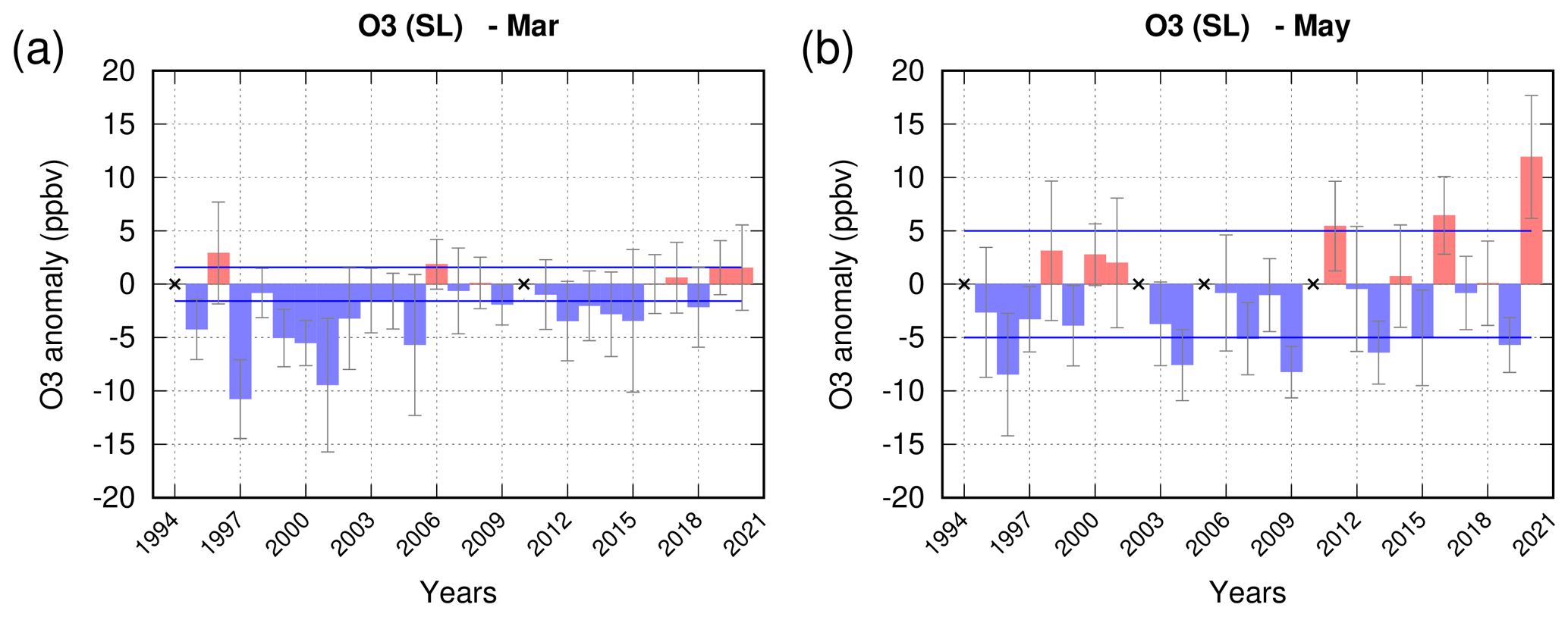
Figure 2Anomalies of ozone for 1994–2020 calculated with respect to 2016–2019 for the months of (a) March and (b) May for the surface layer (>950 hPa; SL). There were no ozone data in April 2020. The grey bars represent the 95 % confidence limits, and the blue horizonal lines represent the interannual variability.
In Fig. 2, we present the anomalies in ozone for the individual months of March and May 2020. As mentioned above, we did not have any ozone data in April 2020. We require there to be 7 d to make the monthly average; otherwise the month is excluded. Excluded months are marked with a cross. During the lockdown period, there were fewer flights than normal, and we need to be aware of any sampling bias that this may introduce. The number of profiles per month is shown as the solid grey bars in top panel of Fig. 3. The confidence limits, shown in Fig. 2, account for the differing number of profiles per month. The confidence limits are calculated using Student's t distribution.
It was during the month of May, after the lockdown had been in place for several weeks, that the ozone anomaly in the surface layer (pressure P>950 hPa) was most pronounced (Fig. 2). In May, ozone was recorded at +11.9 ppbv (+32 %) higher than the reference average (2016–2019) and was the largest anomaly for the month of May since the time series began in 1994. The magnitude of the anomaly including the 95 % confidence limits is outside the interannual variability, based on the reference years, given by the solid blue line. The anomaly is apparent in the first 1000 m of the atmosphere (Fig. 1). A positive anomaly was also observed in March 2020 (5 %) with a smaller value compared with May. Positive anomalies in ozone have not been unusual in recent years (see Fig. 3), suggesting that the lockdowns are not the only explanation.
To set the magnitude of these anomalies into context with other periods, the time series for each month for the surface layer over Frankfurt is shown in the bottom panel of Fig. 3. The anomalies are calculated with respect to 2016–2019. There were a few occasions when the ozone anomalies were comparable to that of May 2020 including a peak of similar magnitude in February 2005. In the other seasons, the peaks were August 2015 and September 2016 when there were short heatwaves and the well-known heatwave in August 2003 which we discuss here, as it was well documented with IAGOS data (Tressol et al., 2008; Ordóñez et al., 2010). It should be noted that, when compared with the recent reference period of 2016–2019, the magnitude of the anomaly in August 2003 is diminished, suggesting that these high ozone abundances have become less unusual.
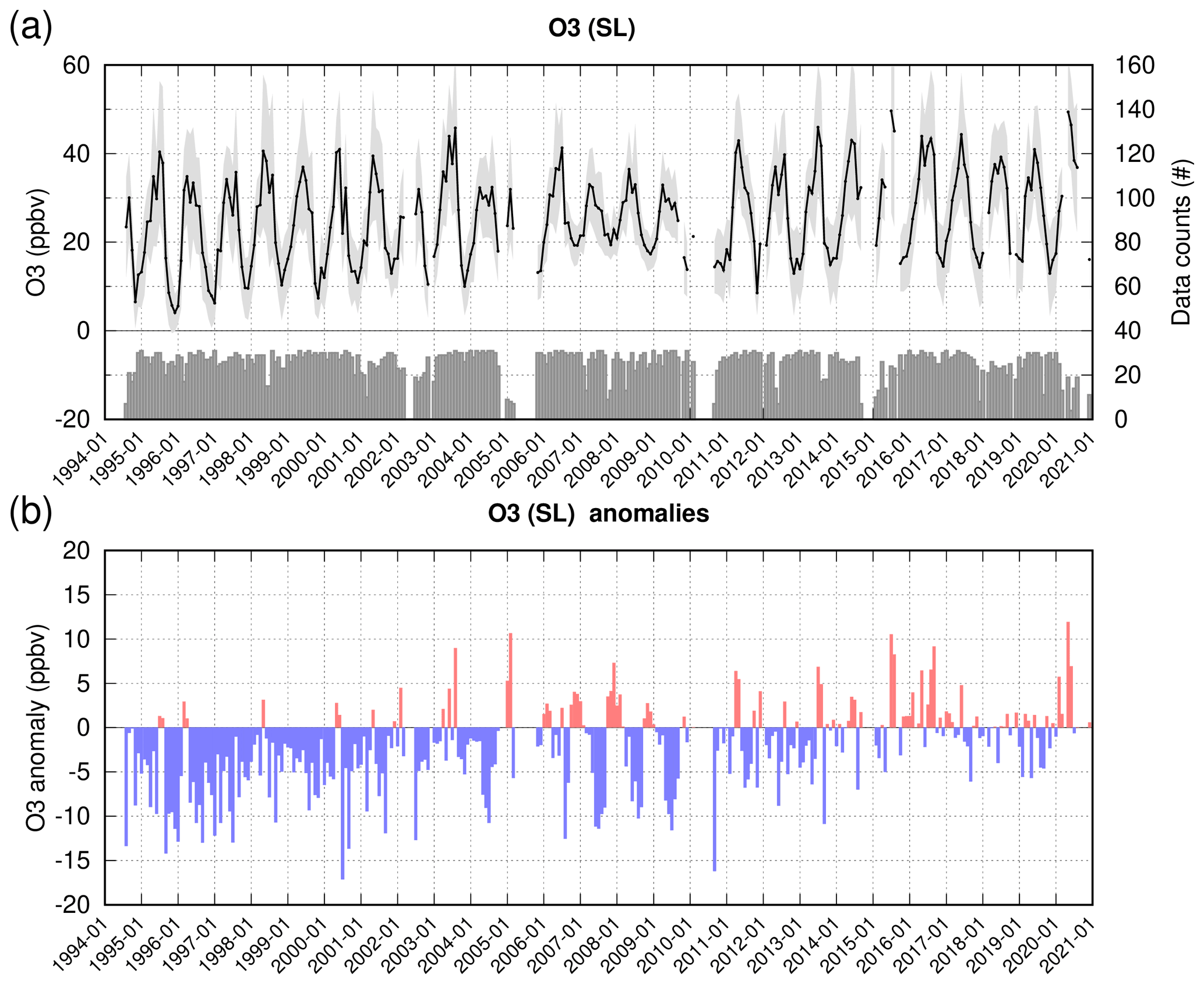
Figure 3Monthly time series for 1994–2020 of O3 for the surface layer over Frankfurt (a). The grey bars represent the number of daily profiles used to calculate the monthly means shown in black. Grey shading represents the standard deviation for each month. (b) The monthly anomalies calculated with respect to the reference average of 2016–2019 in the surface layer. Please note that the date format used in this figure is yyyy-mm.
An increase in ozone near the surface can result from increased production of ozone or reduced sinks of ozone, depending on the conditions and the time of day. Positive anomalies of ozone may be due to an increase in the precursors of ozone or a prevalence of certain meteorological conditions including increased UV radiation, stagnant air masses or lower boundary layer heights which trap the pollutants near the surface. Otherwise, there can be a decrease in the sinks of ozone, such as a decrease in the rate of dry deposition or a decrease in titration by NO due to a reduction in the emissions of NOx. During the 2003 heatwave, IAGOS data showed that there were positive anomalies at Frankfurt in both ozone and the precursor carbon monoxide in the low troposphere, with the ozone anomalies up to 2.5 km deep and with the magnitude of the anomalies increasing towards the surface (Tressol et al., 2008). Tressol et al. (2008) found that near the surface, ozone was almost twice the normal amount, and CO was more than 20 % higher. The increased CO was due to the transport of plumes from wildfires over Portugal exacerbated by the dry conditions created by the heatwave. Thus, during the 2003 heatwave, the increased ozone was caused by an increase in precursors and the favourable meteorological conditions.
During lockdown, the chemical environment was quite different. The positive anomaly of ozone was accompanied by a drop in the amount of NO as evidenced by the TROPOMI satellite measurements of NO2 (Bauwens et al., 2020), and there is some evidence from IAGOS measurements that levels of the precursor carbon monoxide also fell (see Sect. 4). The anomaly of ozone in the surface layer (extending to 1 km; cf. 2.5 km in the 2003 heatwave) was most likely due to the combination of increased production of ozone due to the exceptionally sunny conditions across a large sector of northern Europe (van Heerwaarden et al., 2021; Ordóñez et al., 2020; see also https://surfobs.climate.copernicus.eu/stateoftheclimate/may2020.php, last access: 3 November 2021) along with the removal of one of the ozone sinks, particularly the reduction in ozone titration because of the reduction in NO. In addition, the stable meteorological conditions, lack of wind and air stagnating over towns could also have contributed to the accumulation of pollutants and of ozone itself in the boundary layer. Some recent studies have attempted to tease out the contribution of meteorology from the impact of the changes in the emissions of precursors (Ordóñez et al., 2020; Petetin et al., 2020; Lee et al., 2020). All found that there were important and differing impacts of meteorology but that there were changes in NOx that were unattributed to the meteorological conditions and linked to falling emissions during the lockdowns.
The magnitude of any anomaly may be significantly influenced by the sampling times within the diurnal cycle. Petetin et al. (2016a) described the typical diurnal cycle of ozone at Frankfurt Airport observed with IAGOS data at different altitudes. They noted that the mixing ratios of ozone are at their minimum at nighttime due to dry deposition and titration by NO in the shallow nocturnal boundary layer and reach a maximum in the afternoon, due to photochemistry and mixing with ozone-rich layers above the boundary layer. Petetin et al. (2016a) showed the diurnal cycle of ozone at Frankfurt to be maximum between 12:00 and 18:00 UTC in MAM in the layers below 900 hPa. The amplitude is at its maximum at the surface and decreases with altitude, becoming almost insignificant at altitudes above 900 hPa. We consider the anomaly observed in May with respect to the diurnal cycle of ozone. More measurements in the afternoon would lead to an oversampling of the maximum and a positive ozone anomaly, and conversely, more measurements at nighttime would be an oversampling of the minimum and a negative anomaly. In Fig. 4, we can see the hourly distribution of the IAGOS profiles for the months of March and May in 2020 compared with the same months in the reference period of 2016–2019. In the climatology, there is a bias towards measurements in early morning. In March 2020, the distribution is similar to that during the reference period, but in May 2020 there is a bias towards measurements in early afternoon. This reflects the different flight operations carried out during the COVID-19 period.
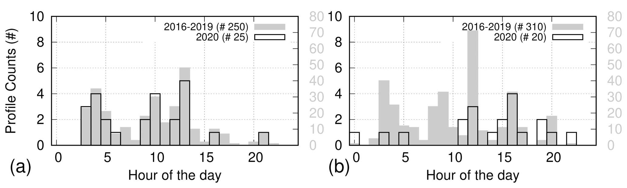
Figure 4Number of profiles by hour of the day (UTC) for (a) March 2020 and (b) May 2020 (counts on left-hand axis) compared with the same months in the reference period of 2016–2019 (counts on right-hand axis).
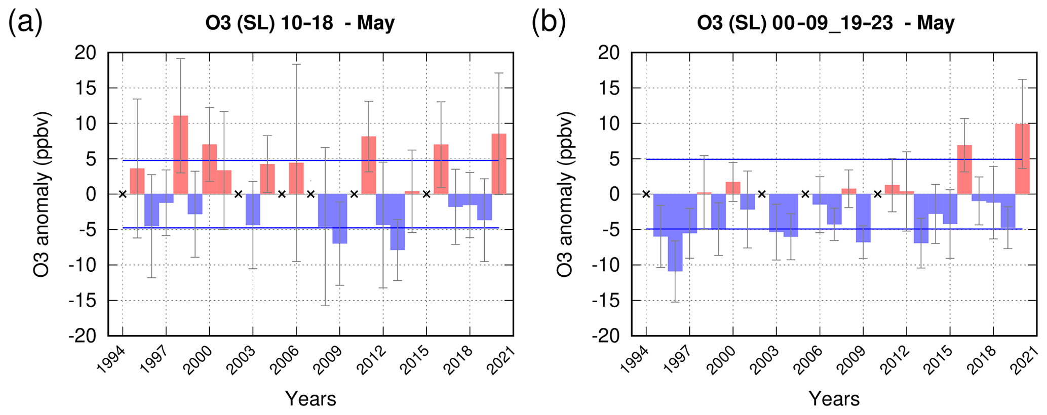
Figure 5Anomalies of ozone for 1994–2020 for the month of May in the surface layer (>950 hPa) for the (a) daytime (10:00–18:59 UTC) and (b) nighttime (00:00–09:59 and 19:00–23:59 UTC). The grey bars represent the 95 % confidence limits, and the blue horizonal lines represent the interannual variability.
To account for this bias, we calculate the anomaly for May for the hours when the diurnal cycle is at its maximum (10:00–18:59 UTC) and the hours when the diurnal cycle is at its minimum (00:00–09:59 and 19:00–23:59 UTC), applying this to both the climatology and 2020 (Fig. 5). This is based on the diurnal cycle for ozone at Frankfurt in MAM described in Petetin et al. (2016a) and depends upon ozone photochemistry and the dynamical development of the boundary layer. In Fig. 5a there remains a significant increase in ozone in May during the day (8.3 ppbv, 19 %), comparable with other anomalies which have occurred four times during the last 26 years. This likely reflects the meteorological conditions that were relatively exceptional and favourable to ozone formation. In Fig. 5b the nighttime increase (9.9 ppbv, 29 %) is clearly the most significant observed in the time series. We infer that the positive anomaly in ozone at nighttime is linked to the drop in NO2 at Frankfurt (Barré et al., 2021) during lockdown and the consequent reduction in ozone titration. Once meteorological changes were accounted for, the estimates of lockdown-induced NO2 changes for Frankfurt were −24 % and −33 % based on TROPOMI observations and surface stations respectively (Barré et al., 2021). The positive ozone anomaly observed in IAGOS data for the surface layer is in agreement with the other studies cited based on the surface networks and as reviewed by (Gkatzelis et al., 2021). The IAGOS data for the remainder of 2020 (Fig. 3) show smaller positive anomalies which were not significant within the time series, suggesting that the anomaly in MAM was short-lived. We now explore the vertical extent of the ozone anomaly, using the unique perspective that IAGOS offers.
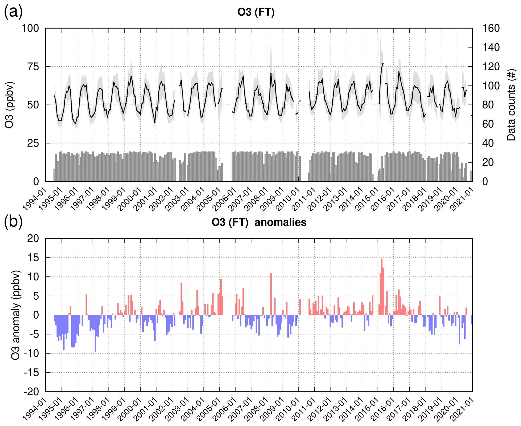
Figure 6Monthly time series for 1994–2020 of O3 for the free troposphere (850–350 hPa; FT) over Frankfurt (a). The grey bars represent the number of daily profiles used to calculate the monthly means shown in black. Grey shading represents the standard deviation for each month. (b) The monthly anomalies calculated with respect to the reference average of 2016–2019 in the free troposphere. Please note that the date format used in this figure is yyyy-mm.

Figure 7Anomalies of ozone for 1994–2020 for the months of (a) March and (b) May in the free troposphere (850–350 hPa). There were no ozone data in April 2020. The grey bars represent the 95 % confidence limits, and the blue horizonal lines represent the interannual variability.
3.2 Anomalies of ozone in the free troposphere (850–350 hPa)
In contrast to the positive anomaly in the surface layer up to 1000 m, the anomaly in the free troposphere above 2000 m is negative (Fig. 1), lying just outside of the range of interannual variability based on the 26-year time series shown in Fig. 6. The grey bars in the top panel of Fig. 6 represent the number of available daily profiles in each month (where there was more than 7 d available in the month). There was a −7.6 ppbv or −14 % change in ozone in March (Fig. 7). This negative anomaly is the largest for March since 1997 for the IAGOS observations in the free troposphere. It is too early to have resulted from the European lockdowns and not easy to link to the Asian lockdowns. There was only a −3.4 ppbv (−5 %) change in ozone in the free troposphere over Frankfurt in May 2020 which might be linked to regional European lockdowns (Fig. 7) but is not outside the interannual variability. We had no data for April 2020. The IAGOS data show that ozone levels remained lower than usual for several months after the main lockdown period ended, with a −10 % anomaly being observed in July (the largest anomaly recorded for July in the 27-year time series; see Fig. A1) as the economic recovery and emissions remained suppressed throughout summer 2020 (Fig. 6). Over the period of April–August 2020, a 7 % drop was seen by ozonesondes (Steinbrecht et al., 2021) from 1–8 km in altitude. This figure represents a mean value across all sites in the Northern Hemisphere over the period of April–August 2020 compared with the 2000–2020 climatology. The negative anomaly seen at Frankfurt in IAGOS data may illustrate that ozone abundances fell widely during MAM due to the combined effect of the lockdown measures across Europe, but evidence from the ozonesondes (Steinbrecht et al., 2021) suggests that we can expect a degree of geographical variability. For example, there was no notable decrease in free-tropospheric ozone in the sparsely sampled Southern Hemisphere.
As mentioned in the Introduction, some studies have demonstrated a fall in the ozone precursors during MAM 2020. The reductions in CO in near-surface air masses due to COVID-19 reported by (Gkatzelis et al., 2021) ranged from 20 % to 50 % for CO. Due to the long (weeks to months) lifetime of CO in the atmosphere, the causes of these decreases in CO are difficult to attribute. Figure 8 shows the seasonally averaged profile of CO measured at Frankfurt for MAM 2020, with the black solid line denoting the IAGOS observations. The red solid line represents the seasonal average for the reference period of 2016–2019, and the red shaded area shows the interannual variability of MAM over the reference period. Often, there are fewer IAGOS observations near the surface than in the free troposphere, which leads to the standard deviation being greater near the surface as shown by the wider envelope (shaded red area). The inflection of the black curve results from a small number of flights which nevertheless fall within the expected range shown by the red shaded area. Despite the length of the time series being nearly 20 years, we have chosen the same short segment (2016–2019) for our reference period as we used for ozone. This is because there is a negative trend in CO (−1.9 % yr−1 and 2.0 % yr−1 from Petetin et al. (2016b) for lower-troposphere and mid-troposphere springtime respectively), and thus all recent data show a negative anomaly (see also Fig. 9). We return to this point later. For the period of MAM 2020 we can see that the CO mixing ratios are below the average for recent years (red line) and lie at the lower limit given by the envelope of interannual variability.
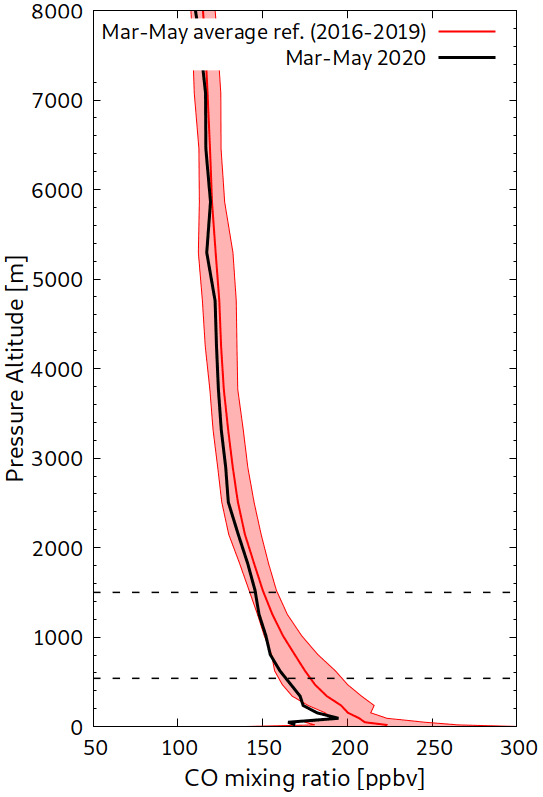
Figure 8IAGOS observations of CO for March–April–May (MAM) 2020 in black. In red, the average profile for MAM calculated over the reference period of 2016–2019 (300 profiles). The shaded area represents the interannual variability for MAM over this reference period. Horizontal lines denote the boundaries of the sections of study as used in subsequent figures.
Similar averaged profiles were presented in Petetin et al. (2016b) based on the period (2002–2012) where the average mixing ratio at 2000 m for MAM was 150 ppbv. For our segment of 2016–2019 the average mixing ratio for MAM at 2000 m was 140 ppbv, indicative of the negative trend of CO. Over the period of 2002–2020, there has been a drop in CO mixing ratios observed at Frankfurt due to a reduction in emissions and the impact of emissions protocols. However, there is a strong interannual variability in the free-tropospheric background which reflects the interannual variability in global biomass burning, anthropogenic emissions, and the complex interactions with other species such as OH and O3. The background abundance of CO therefore depends on the selected segment of the time series.
4.1 Anomalies of carbon monoxide in the surface layer (>950 hPa)
In the surface layer, we see a downward trend in monthly values of CO on the seasonal and annual scale (see Fig. 9) in agreement with Petetin et al. (2016b). Also shown in Fig. 9 is the number of flights per month as the solid grey bars which reveals a reduction in flights due to the reduction in global travel during the first phase of the pandemic. As with ozone, only months where there is at least 7 d are used to make the monthly average; otherwise the month is excluded. The anomalies in Fig. 9 are calculated with respect to the short reference time series of 2016–2019. In 2020, we can see a drop in CO mixing ratios with the lowest values in the time series being recorded in February 2020.
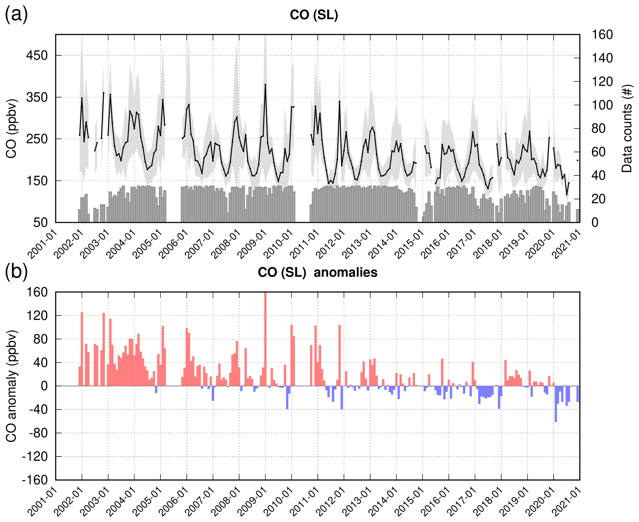
Figure 9Monthly time series for 2001–2020 of CO for the surface layer over Frankfurt (a). The grey bars represent the number of daily profiles used to calculate the monthly means shown in black. Grey shading represents the standard deviation for each month. (b) The monthly anomalies calculated with respect to the reference average of 2016–2019 in the surface layer. Please note that the date format used in this figure is yyyy-mm.

Figure 10Anomalies of CO for 2001–2020 for the months of (a) March, (b) April and (c) May, in the surface layer (>950 hPa). The grey bars represent the 95 % confidence limits, and the blue horizonal lines represent the interannual variability.
Figure 10 shows the anomalies for March, April and May for 2001–2020. In May, towards the end of the lockdown period, the anomaly was (−27.2 ppbv, −15 %), and the 95 % confidence limit is outside the range of interannual variability. However, inspection of the time series (Fig. 9) reveals that the greatest anomaly relative to 2016–2019 was actually apparent in February, before the European lockdown measures began. When compared with the reference time series (2016–2019), the anomaly in February was (−61.4 ppbv, −26 %; see Appendix Fig. B1). February lies outside our main period of interest, but the large anomaly observed then suggests that the drop in CO at the surface observed in subsequent months is not wholly attributed to the drop in emissions linked to lockdown. Indeed, a fall in NO2 levels was also reported by Peuch (2020) from February onwards. Peuch (2020) suggested that the driver of this could be an increase in boundary layer heights and consequent dilution of the pollutants near the surface. To investigate if this could be a factor in the low CO seen in IAGOS data, we examine the boundary layer heights for 2020 compared with the 2016–2019 average.
We calculated the boundary layer height (the boundary layer height (BLH) is the boundary layer thickness (zPBL) plus orography) by interpolating the ECMWF operational boundary layer heights to the position of the IAGOS aircraft. The ECMWF fields had a 1∘ horizontal resolution and 3 h time resolution. We used a bilinear interpolation in space using a distance weighting from the four nearest grid cells to the IAGOS position and a linear interpolation in time. This calculated BLH is one of a number of added-value products which are included with IAGOS data as a standard in “level 4”. Due to the diurnal variability of the boundary layer height as the convective boundary layer develops during the day and the seasonal variability in the time of sunrise and sunset, Fig. 11 is divided into two time slots. The top panel shows the afternoon–evening, defined as 3 h after sunrise until 2 h before sunset. The bottom panel shows the nighttime–morning defined as 2 h before sunset until 3 h after sunrise. Each time series shows the percentage difference with respect to the monthly mean calculated for 2016–2019 and is shown for 8 months (January–August) for each year between 2016 and 2020. The depth of the nighttime boundary layer increased by 60 % (400 m) in February and 70 % in May with respect to the monthly mean from 2016–2019 and was greater than any other anomaly observed over the period of 2016–2019. The anomaly covers the MAM period and may partly explain the decreased concentrations of CO in the surface layer. We accounted for these changes by integrating the CO over the height of the boundary layer. A negative anomaly of 30 ppbv in February and of 12 ppbv in March and May was noted which can be ascribed to decreases in emissions.
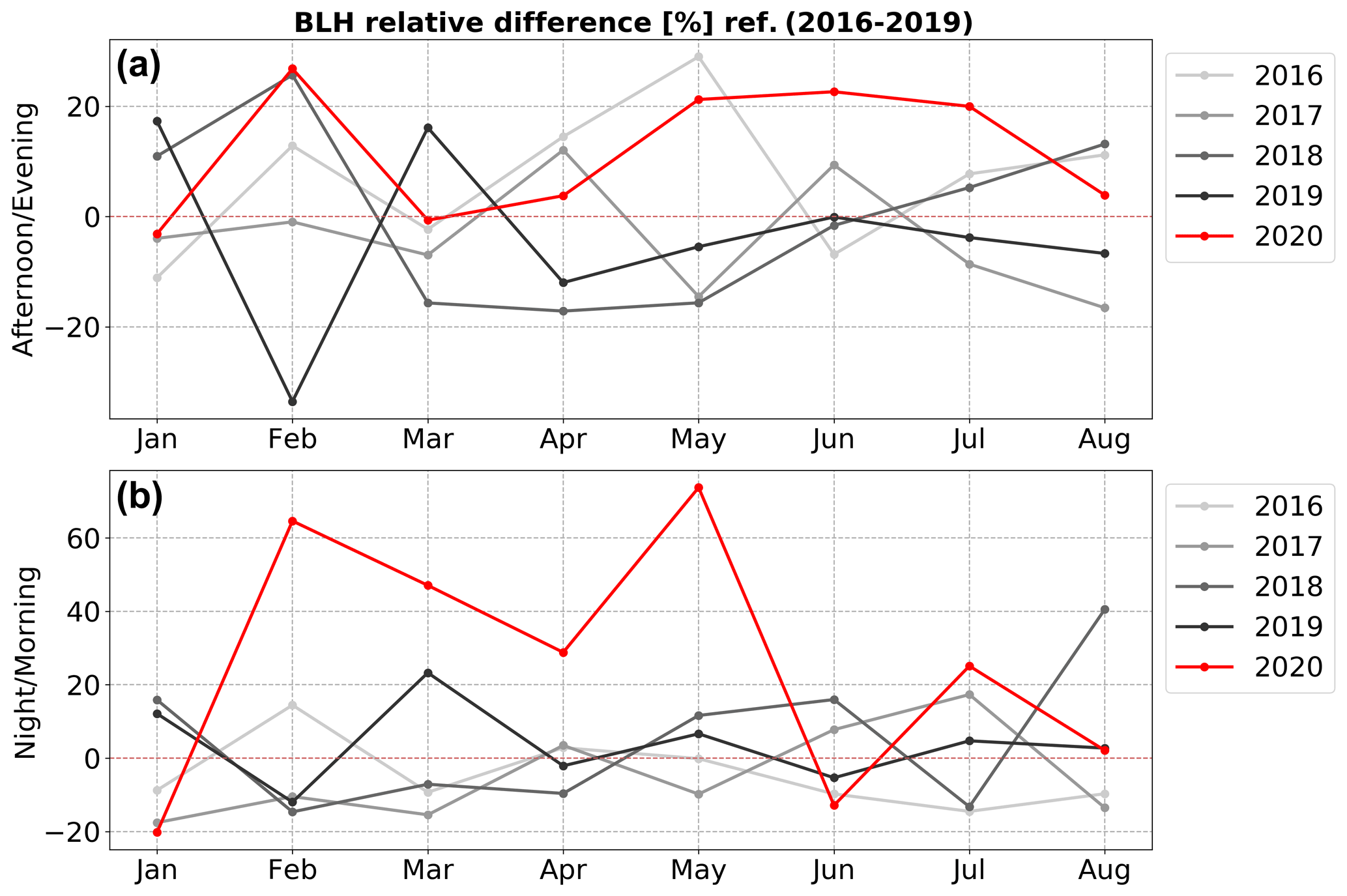
Figure 11Monthly averaged boundary layer heights interpolated in space and time from the 3-hourly ECMWF operational fields on 1∘ resolution for afternoon–evening (a) and nighttime–morning (b). Afternoon–evening is defined as 3 h after sunrise until 2 h before sunset, and nighttime–morning is defined as 2 h before sunset until 3 h after sunrise. The boundary layer heights are expressed as a percentage difference from the mean height calculated over the period of 2016–2019.
The observations of CO near the surface from IAGOS are less impacted by the local emissions at airports than might be thought. Petetin et al. (2018a) compared IAGOS with monitoring stations from the local air quality monitoring network (AQN) and more distant regional surface stations from the Global Atmospheric Watch (GAW) network. They found that the mixing ratios of CO and O3 close to the surface do not appear to be strongly impacted by local emissions related to airport activities and are not significantly different from those mixing ratios measured at surrounding urban background stations. It is therefore unlikely that the reduction in airport activity during COVID-19 was a big contributor to the negative anomaly observed at Frankfurt in the surface layer. In the free troposphere, the local emissions have even less effect, and the mixing ratios tend to background concentrations as typically measured by the GAW regional stations.

Figure 12Emissions regions used for the SOFT-IO v1.0 model. BONA: Boreal North America; TENA: Temperate North America; CEAM: Central America; NHSA: Northern Hemisphere South America; SHSA: Southern Hemisphere South America; EURO: Europe; MIDE: Middle East; NHAF: Northern Hemisphere Africa; SHAF: Southern Hemisphere Africa; BOAS: Boreal Asia; CEAS: Central Asia; SEAS: Southeast Asia; EQAS: Equatorial Asia; AUST: Australia and New Zealand.

Figure 13Contribution from different source regions to the CO in the surface layer at Frankfurt in MAM 2020 compared with MAM 2016–2019. The colours correspond to the regions in Fig. 12.
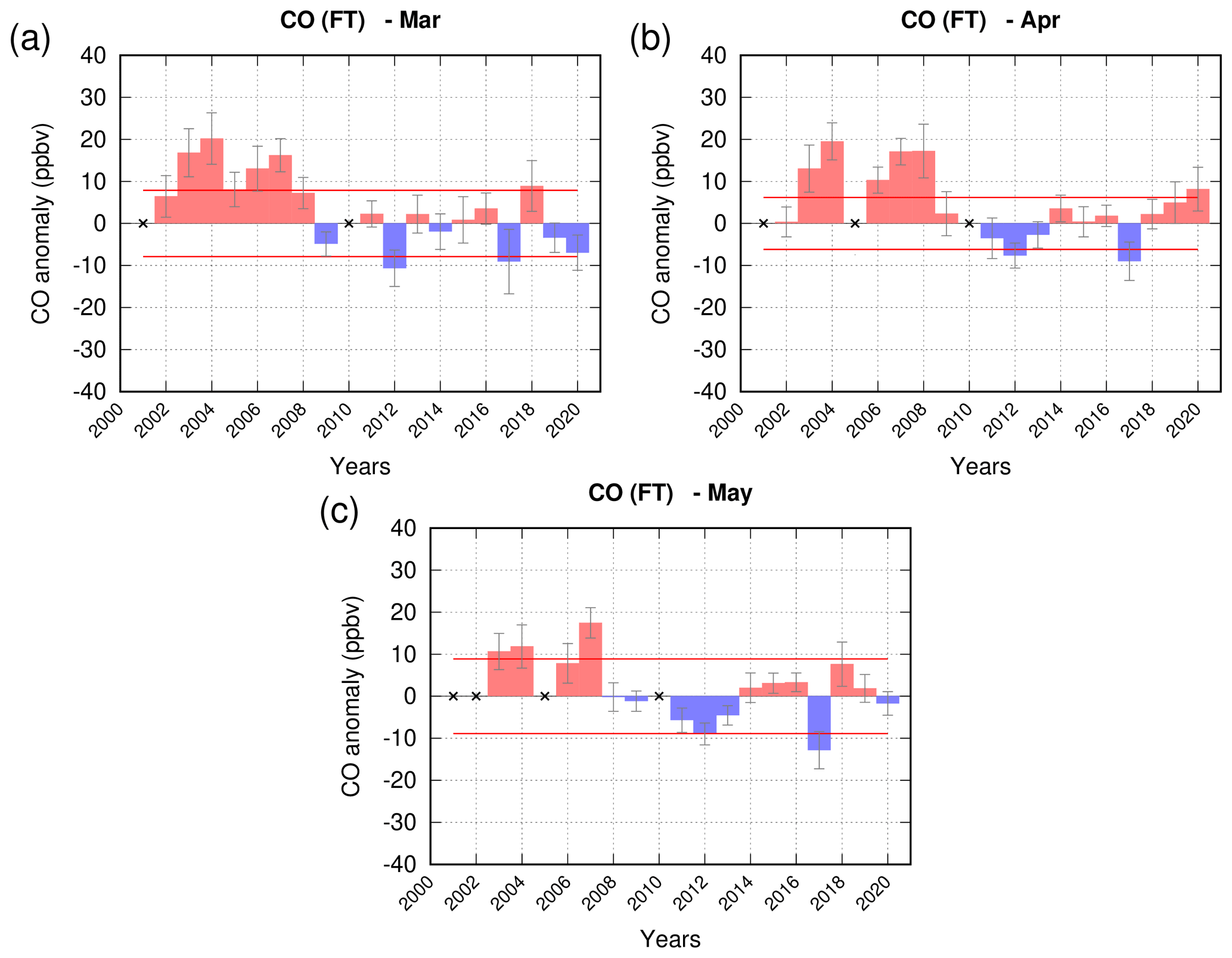
Figure 14Anomalies of CO for 2001–2020 for the months of (a) March, (b) April and (c) May, in the free troposphere (850–350 hPa). The grey bars represent the 95 % confidence limits, and the blue horizonal lines represent the interannual variability.
To examine more closely the source regions of the CO at Frankfurt, we have used the SOFT-IO tool which routinely connects emissions databases to each IAGOS measurement via FLEXPART trajectory calculations (Sauvage et al., 2017b, 2018). SOFT-IO does not calculate the background amounts of CO which include CO from emissions older than 20 d or secondary CO produced by chemical reactions in situ. It is more adapted to look at well-defined plumes of pollution visible against the background. In addition, the anthropogenic emissions database (MACCity; Monitoring Atmospheric Composition and Climate) has not been updated to take account of the COVID-19 period. This makes the relative contribution from each source difficult to determine. For these reasons we will focus on the geographic origin of the CO at Frankfurt as determined by the trajectory calculations. The source regions are defined as in Fig. 12. The trajectories terminate at the aircraft position within the surface layer. We compare the source regions in 2020 with those in our reference period of 2016–2019. In Fig. 13, we show the source region of the emissions. In agreement with Petetin et al. (2018b), our analysis shows that the largest contribution to CO measured at Frankfurt is from the European region. Usually in this period, the contribution from biomass-burning emissions to the surface CO is small. In 2020, there was a smaller absolute contribution to the surface CO from biomass-burning emissions (1.3 ppbv in 2020 compared with 2.7 ppbv in 2016–2019) with the relative contribution being 10 % in the reference period. Most of the emissions in Europe in 2020 were therefore anthropogenic. The majority (70 %) of the CO at Frankfurt had a European origin in both 2020 and in the reference period of 2016–2019. In 2020, there was a greater contribution from sources in North America (TENA and BONA) and Asia (CEAS) compared with 2016–2019, which reflects the interannual variability of different air masses arriving in Europe. This analysis shows that it is primarily local emissions across Europe that are reflected in the CO recorded at Frankfurt in the surface layer, and therefore we can suppose that the lockdown measures played a significant role. In the free troposphere, which we discuss in the following section, we will see that inter-continental transport has a more important contribution.
4.2 Anomalies of carbon monoxide in the free troposphere (850–350 hPa)
In the free troposphere, the anomalies of CO (Fig. 14) were negative in March (−6.9 ppbv, −5 %) and May (−1.8 ppbv, −1 %) but much smaller in magnitude than in the surface layer (see Sect. 4.1) and do not exceed interannual variability once the confidence limits have been considered. The time series of CO in the free troposphere from 2001–2020 is included for reference in Fig. B2. In April, the anomaly was positive (8.2 ppbv, 6 %). Since the free troposphere is more representative of the background concentrations due to mixing and transport, it is instructive to relate the IAGOS data over Frankfurt to the larger geographical context. Satellite fields of CO in the tropospheric column are presented for Europe in Fig. 15. Figure 15 represents the percentage change in the tropospheric CO at 795 hPa with respect to the 2016–2019 average as retrieved from IASI for the months of March, April and May. In March, the IASI-SOFRID data confirm the negative anomaly in CO present at Frankfurt, which is generalized over large parts of Europe. In April and May, the IASI-SOFRID data showed little anomaly at Frankfurt and a mixed picture over Europe. Thus, the IAGOS and IASI data show some reduction in CO during the lockdown period which is not unexpected given the trend towards decreased CO. It is difficult to link this anomaly to the lockdown measures due to other factors such as the increased boundary layer height, the long-range global transport of CO and interannual variability.
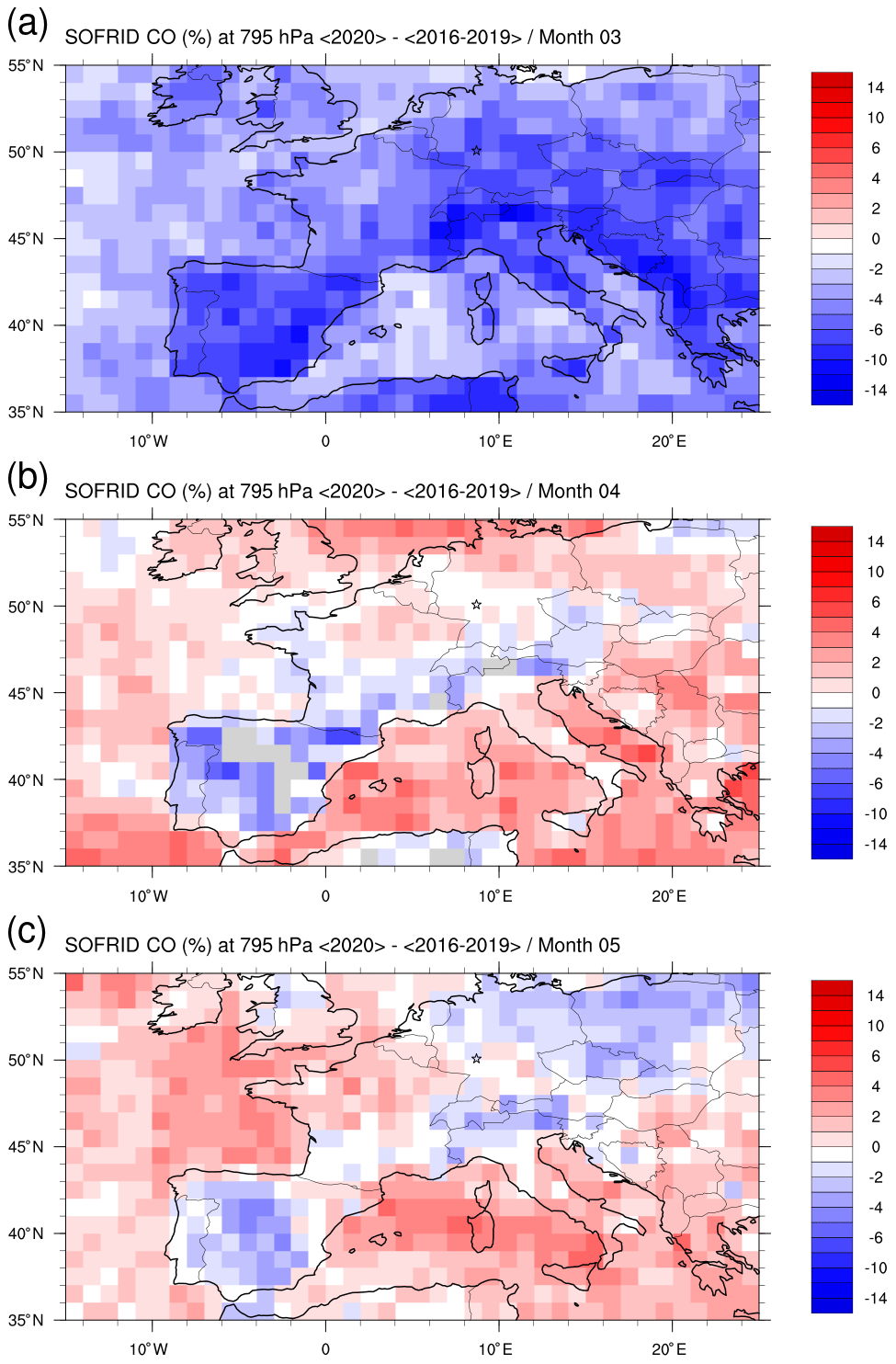
Figure 15Percentage change of IASI-SOFRID carbon monoxide at 795 hPa in (a) March, (b) April and (c) May 2020 compared with the reference average period of 2016–2019.
Using the same trajectory analysis as for Fig. 13, Fig. 16 shows that in MAM 2020, there was a much lower amount of CO from sources in Europe than in MAM 2016–2019 and an increase in the contribution from North America (TENA) and from Central Asia (CEAS). We suggest that the increase in air masses carrying CO from anthropogenic and biomass-burning sources from outside Europe offset the effects of the cut in emissions during the European lockdown resulting in a smaller-than-anticipated negative anomaly observed by both IAGOS and IASI-SOFRID. This result is similar to that of Field et al. (2020), who noted only a 2 % change in background abundances of CO over eastern China despite the cut in industrial emissions during the Chinese lockdown. In the case of Field et al. (2020) it was the cross-border transport from areas with active biomass burning that offset the drop in anthropogenic emissions. In our reference period, the mean biomass-burning contributions to the anomaly were about 3 ppbv or 20 %, whereas in 2020, the contribution was 2 ppbv. As the contribution from biomass burning is small in Europe in MAM, the main influence to the CO loading over Europe is from anthropogenic emissions from several source regions with more or less stringent lockdown measures.
In summary for this section on CO, we conclude that the drop in surface CO is largely the result of the drop in emissions during European lockdown, with higher than usual boundary layer heights further diluting the surface concentrations. In the free troposphere, where the negative anomalies were not outside expected interannual variability, the influence of long-range transport is more apparent and offsets the impact of the reduction in CO emissions across Europe.
In this article, we use the IAGOS dataset of in situ observations of ozone and carbon monoxide collected during landing and take-off at Frankfurt Airport. The atmosphere is sampled from the surface to the upper troposphere, forming a quasi-vertical profile. The data form part of a time series which extends back for 27 years for ozone and 20 years for CO. We considered whether anomalies of ozone and CO at Frankfurt during MAM 2020 were related to changes in atmospheric composition resulting from the COVID-19 lockdowns, which reduced the industrial and traffic emissions of ozone precursors (e.g. Bauwens et al., 2020; Barré et al., 2021). We compared MAM 2020 with a baseline period of 2016–2019 to account for recent increases in ozone and decreases in CO. During MAM 2020, we noted a 19 % increase in ozone in the surface layer (>950 hPa, 600 m). The month of May saw a significant anomaly (32 %), the largest since the time series began in 1994.
There was a large increase in ozone in the daytime in May 2020 (19 %), but the increase at nighttime (29 %) was even larger and has not been seen before in the 26-year time series. Despite the fall in the abundance of NOx over Europe (as seen by satellite data), there were still enough available precursors to produce ozone under the meteorological conditions, especially enhanced solar radiation, that were very favourable at the time (van Heerwaarden et al., 2021). The larger increase at nighttime, along with the observation that NO2 fell by between 24 % and 33 % (Barré et al., 2021), suggests that less ozone was lost through titration with NO due to the reduction in the NO reservoir during the lockdown period, signifying a reduction in one of the sinks of ozone. Furthermore, we noted an increase in the depth of the nighttime boundary layer, which would be expected to further reduce the sinks of ozone through less titration and deposition.
The magnitude of this anomaly is comparable to that during the European heatwave in August 2003 which was one of the most significant air quality events in Europe (e.g. Tressol et al., 2008). When compared with the recent reference period of 2016–2019, the magnitude of the anomaly in August 2003 is diminished, suggesting that these high ozone abundances are no longer unusual. Although the anomalies of ozone were of similar magnitude to those during the 2003 heatwave, the chemical environment during the lockdown period was quite different. During the 2003 heatwave, IAGOS data showed that there were positive anomalies at Frankfurt in both ozone and the precursor carbon monoxide in the low troposphere (Tressol et al., 2008). The increased CO was due to the transport of plumes from wildfires over Portugal exacerbated by the dry conditions created by the heatwave. Thus, during the 2003 heatwave, the increased ozone caused the favourable meteorological conditions and an increase in precursors, whereas during lockdown, the positive anomaly of ozone was accompanied by favourable meteorology and a fall in precursors.
In the free troposphere, ozone abundances fell slightly. For the period of MAM 2020 ozone was 10 % lower than the mean of 2016–2019 based on the same months. The IAGOS time series shows that these free-tropospheric abundances of ozone were the lowest since 1997, which is probably more reflective of the widespread reduction of emissions over Europe and beyond, with less of an impact from local meteorology and chemistry. The results from IAGOS are also consistent with those from the balloon-borne ozonesondes reported by Steinbrecht et al. (2021), who noted a 7 % drop in tropospheric ozone compared with the 2000–2020 climatological mean. They also attributed this to the reduction in pollution during the COVID-19 lockdowns.
A reduction in CO was seen at Frankfurt, with an 11 % reduction found in the surface layer but no anomaly in the free troposphere as averaged over MAM. The attribution of this decrease to the drop in emissions during lockdown is complicated by the fact that the boundary layer heights were anomalously high during this period and might therefore have contributed to a dilution of the CO at the surface. However, the negative anomalies persist despite controlling for this. It should be noted that the greatest decrease in CO occurred in February (26 %), before lockdown measures had been introduced in Europe. Our trajectory analysis shows that the CO is largely of European origin, and therefore we suggest the impact of the lockdown on abundances of CO is likely.
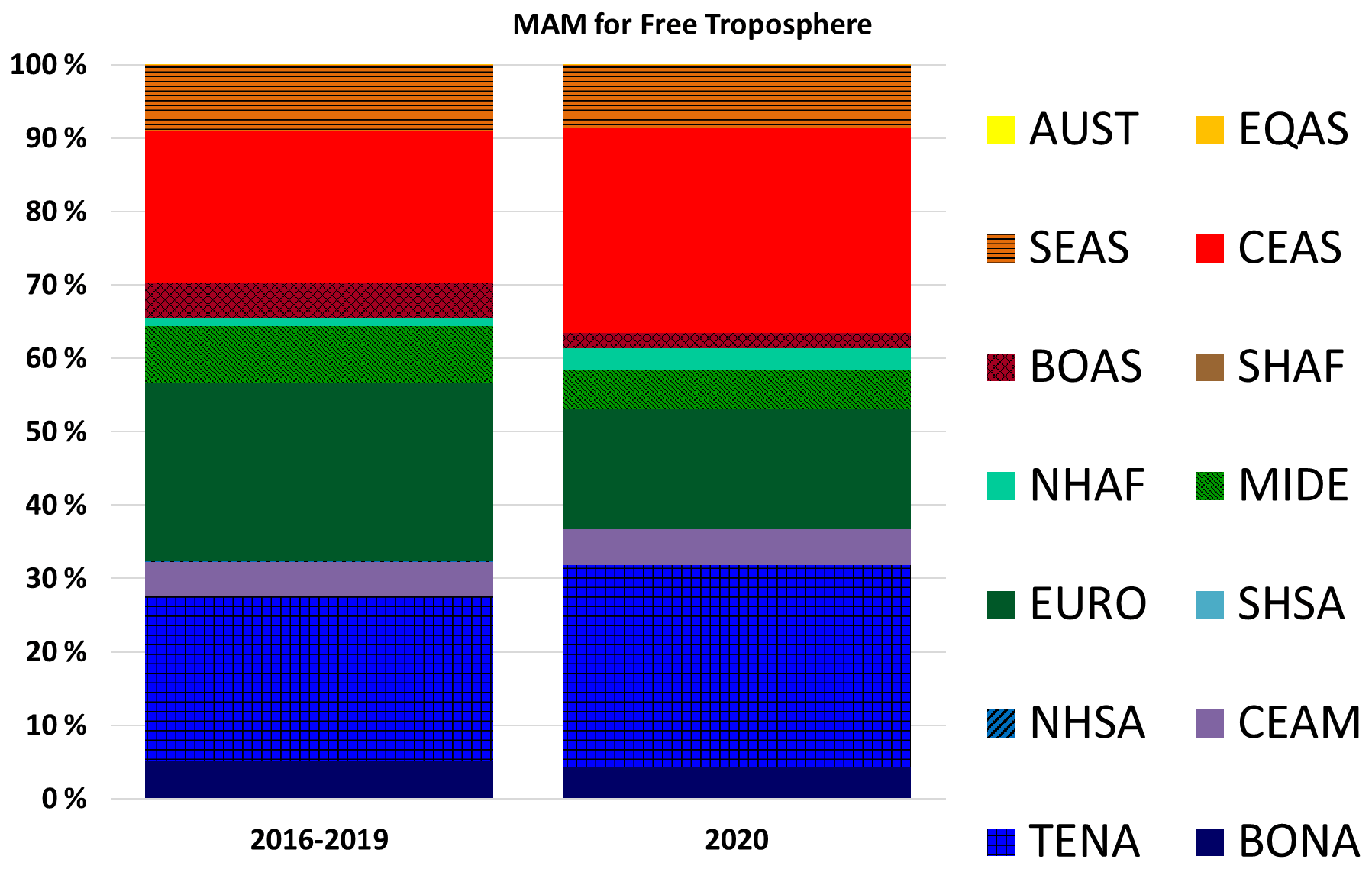
Figure 16Contribution from different source regions to the CO in the free troposphere at Frankfurt in MAM 2020 compared with MAM 2016–2019. The colours correspond to the regions in Fig. 12.
In the free troposphere there is a small reduction in CO in March (−6.9 ppbv, −5 %) and May (−1.8 ppbv, −1 %) which is smaller than at the surface over Frankfurt and remains within the range of interannual variability. IASI-SOFRID fields of CO show a clear decrease in CO during March over all of Europe. In April and May small positive and negative anomalies over northern Europe and mostly negative anomalies over the Iberian Peninsula are detected by IASI-SOFRID. In the free troposphere, there is an important role of transport of CO from distant biomass and anthropogenic sources. In particular in MAM 2020, there was a greater contribution from CO originating in North America and Asia. The contribution by air masses from outside Europe may have offset some of the drop in CO resulting from the reduction in regional European emissions, with the result that the lockdown measures did not have a big impact on CO in the free troposphere.
The lockdowns provided a unique experiment to assess the impact of a reduction of economic activities on atmospheric composition and climate. The IAGOS data complement other in situ data from the ozonesonde network, with the added value of having ozone precursors measured simultaneously. This study demonstrates the importance of long and continuous time series in setting this brief period in context, since there are many competing factors, and it is difficult to attribute a single cause. We have considered various meteorological factors for both ozone and CO near the surface and for interannual variability and long-range transport in the free troposphere. We look forward to future model sensitivity studies to separate these factors and to provide a more realistic magnitude of the impact of lockdown on the environment.
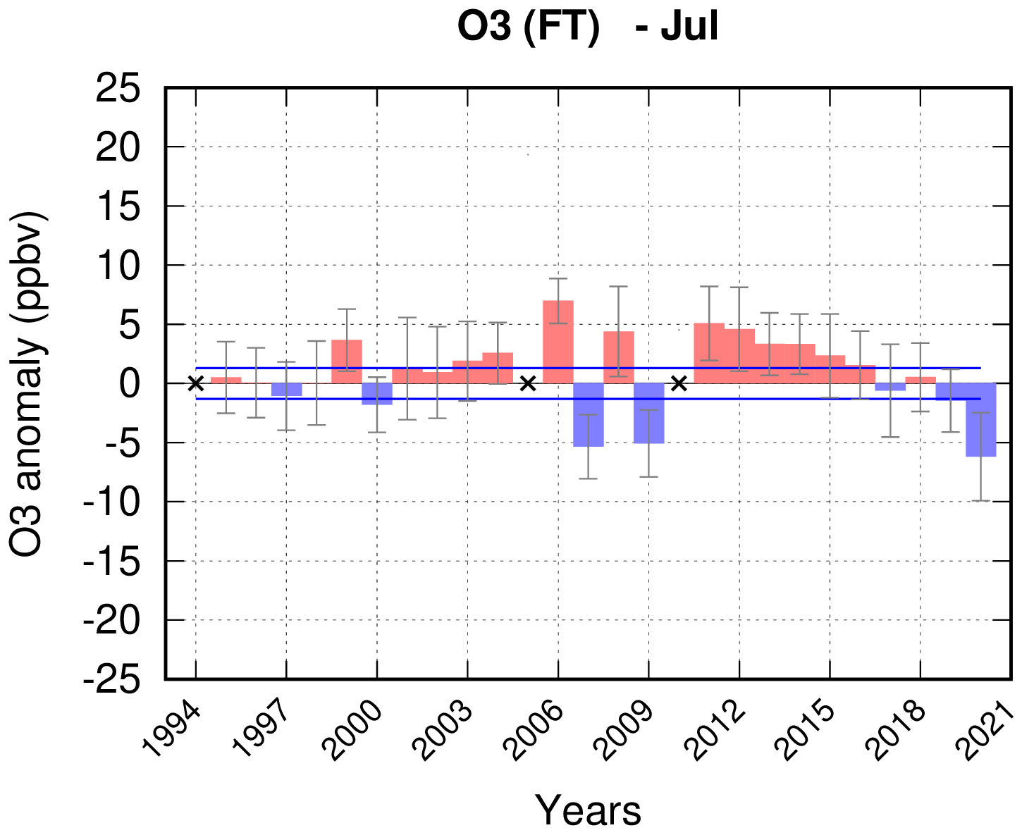
Figure A1Ozone anomalies in the free troposphere (830–350 hPa) for the month of July since 1994. The grey bars represent the 95 % confidence limits, and the blue horizonal lines represent the interannual variability.
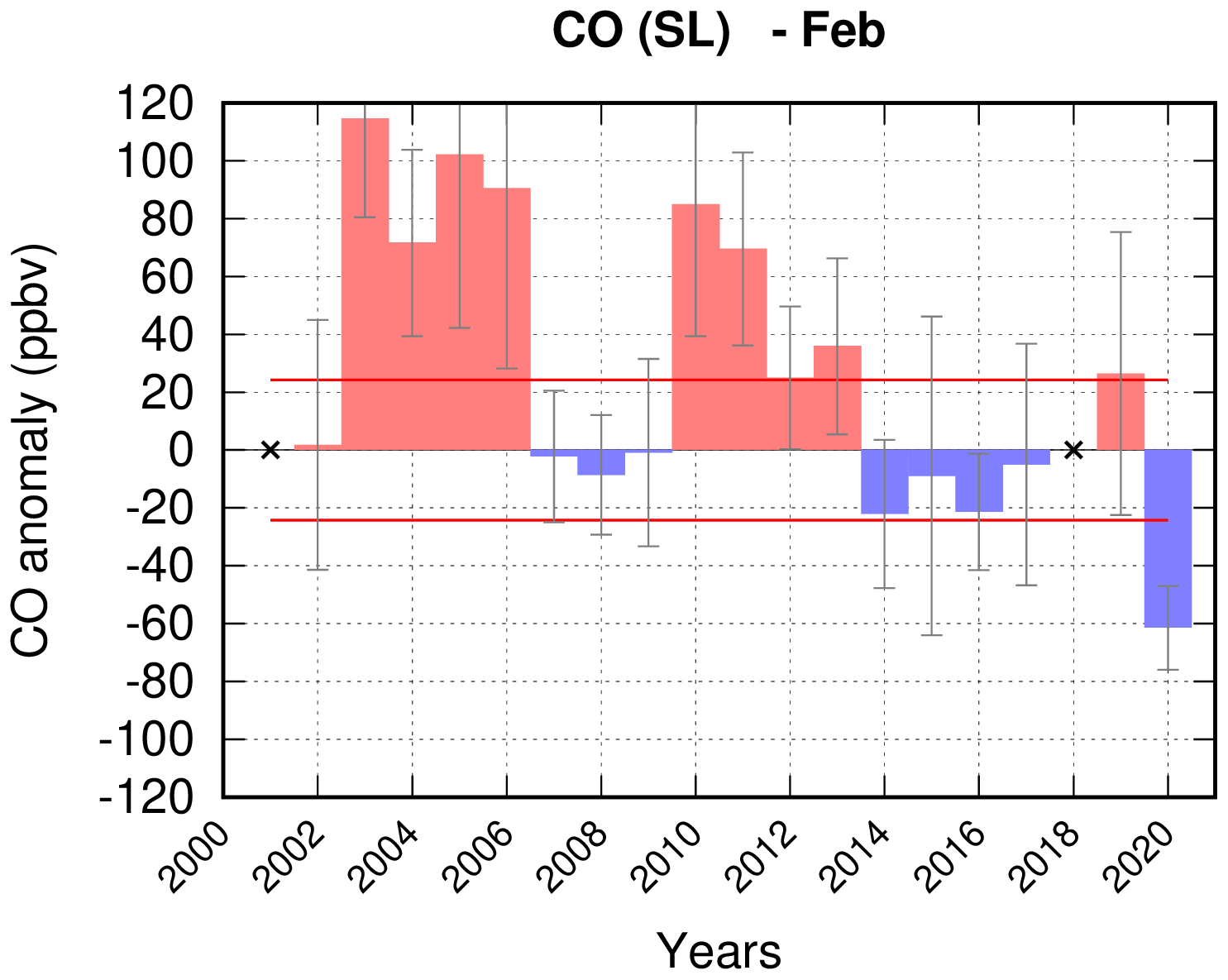
Figure B1Anomalies of CO in the surface layer (>950 hPa) for the month of February since 2001. The grey bars represent the 95 % confidence limits, and the blue horizonal lines represent the interannual variability.
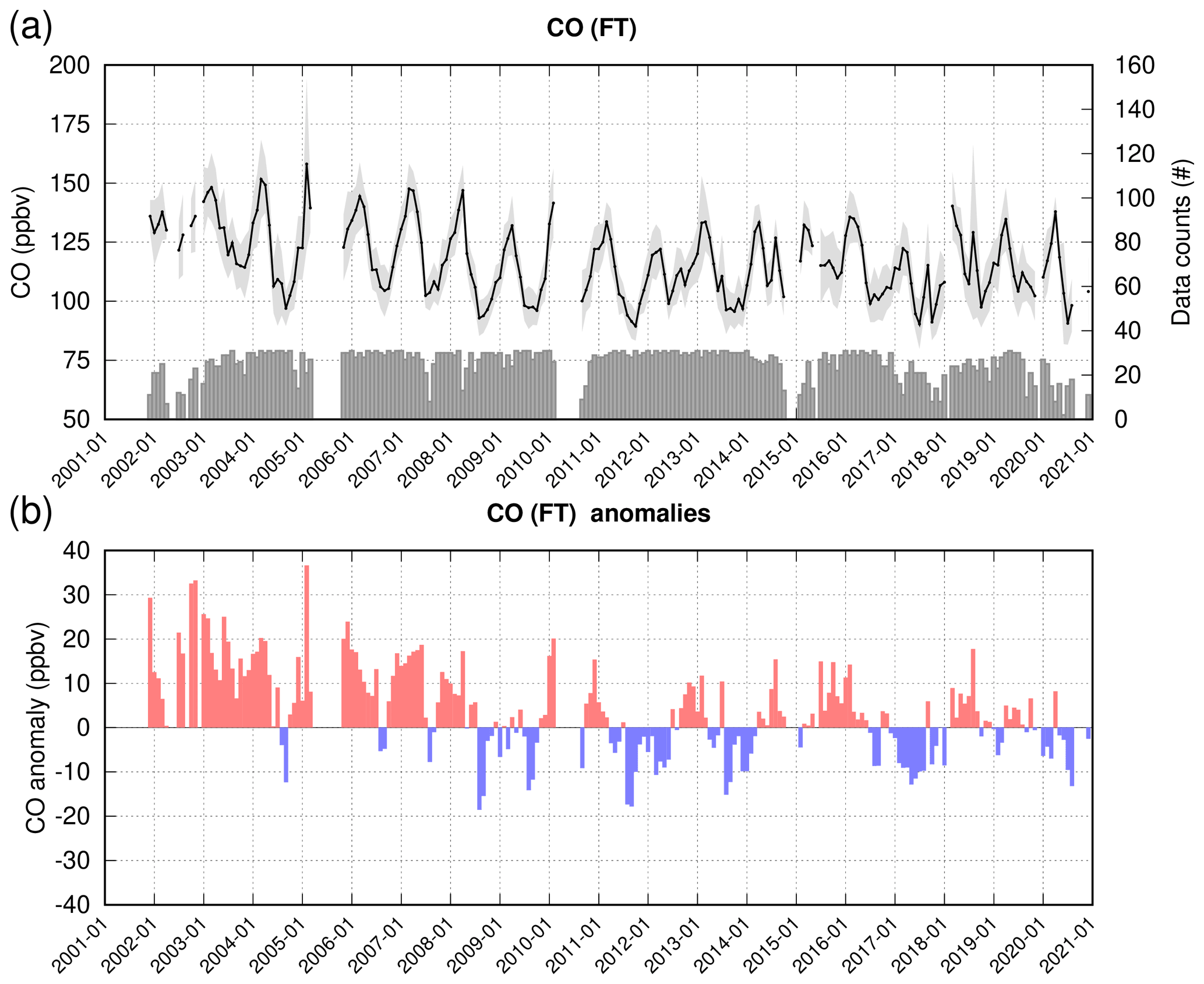
Figure B2Monthly time series for 2001–2020 of CO for the free troposphere over Frankfurt (a). The grey bars represent the number of daily profiles used to calculate the monthly means shown in black. Grey shading represents the standard deviation for each month. (b) The monthly anomalies calculated with respect to the reference average period of 2016–2019 in the free troposphere (830–350 hPa). Please note that the date format used in this figure is yyyy-mm.
The IAGOS data are available through the IAGOS data portal at https://doi.org/10.25326/20 (Boulanger et al., 2021). The IAGOS time series dataset used for this analysis is referenced at https://doi.org/10.25326/06 (Boulanger et al., 2018). The SOFRID O3 and CO data are freely available on the IASI-SOFRID website (http://thredds.sedoo.fr/iasi-sofrid-o3-co/) (SEDOO, 2014).
HC, YB and VT designed the study and prepared the paper with contributions from all co-authors. YB developed the code in the framework of the CAMS-84 (Copernicus Atmosphere Monitoring Service) project. MT, PW and BS are responsible for the level 4 value-added products. PN, RB and JMC produced, validated and calibrated the IAGOS data. DB develops and maintains the IAGOS database. EF and BB performed the IASI-SOFRID retrievals. HC, YB, BS, PN, VT and AP reviewed and edited.
Some authors are members of the editorial board of Atmospheric Chemistry and Physics. The peer-review process was guided by an independent editor, and the authors have also no other competing interests to declare.
Publisher's note: Copernicus Publications remains neutral with regard to jurisdictional claims in published maps and institutional affiliations.
IAGOS has been funded by the European Union projects IAGOS-DS (Design Study) and IAGOS-ERI (European Research Infrastructure). The IAGOS database is supported in France by AERIS (https://www.aeris-data.fr, last access: 3 November 2021). We acknowledge the strong support of the European Commission, Airbus and the airlines (Deutsche Lufthansa, Air France, Cathay Pacific, Iberia, China Airlines and Hawaiian Airlines) that carry the IAGOS equipment. In particular we would like to thank Deutsche Lufthansa for operating D-AIKO in a cargo configuration during the COVID-19 period. IASI is a joint mission of EUMETSAT and the Centre National d'Etudes Spatiales (CNES, France). The authors acknowledge the CNES for financial support for the IASI activities and the Bonus Stratégique programme at Université Toulouse III - Paul Sabatier who fund Maria Tsivlidou.
This paper was edited by Bryan N. Duncan and reviewed by two anonymous referees.
Akritidis, D., Katragkou, E., Zanis, P., Pytharoulis, I., Melas, D., Flemming, J., Inness, A., Clark, H., Plu, M., and Eskes, H.: A deep stratosphere-to-troposphere ozone transport event over Europe simulated in CAMS global and regional forecast systems: analysis and evaluation, Atmos. Chem. Phys., 18, 15515–15534, https://doi.org/10.5194/acp-18-15515-2018, 2018. a
Baldasano, J. M.: COVID-19 lockdown effects on air quality by NO2 in the cities of Barcelona and Madrid (Spain), Sci. Total Environ., 741, 140353, https://doi.org/10.1016/j.scitotenv.2020.140353, 2020. a
Barré, J., Petetin, H., Colette, A., Guevara, M., Peuch, V.-H., Rouil, L., Engelen, R., Inness, A., Flemming, J., Pérez García-Pando, C., Bowdalo, D., Meleux, F., Geels, C., Christensen, J. H., Gauss, M., Benedictow, A., Tsyro, S., Friese, E., Struzewska, J., Kaminski, J. W., Douros, J., Timmermans, R., Robertson, L., Adani, M., Jorba, O., Joly, M., and Kouznetsov, R.: Estimating lockdown-induced European NO2 changes using satellite and surface observations and air quality models, Atmos. Chem. Phys., 21, 7373–7394, https://doi.org/10.5194/acp-21-7373-2021, 2021. a, b, c, d, e
Barret, B., Le Flochmoen, E., Sauvage, B., Pavelin, E., Matricardi, M., and Cammas, J. P.: The detection of post-monsoon tropospheric ozone variability over south Asia using IASI data, Atmos. Chem. Phys., 11, 9533–9548, https://doi.org/10.5194/acp-11-9533-2011, 2011. a
Bauwens, M., Compernolle, S., Stavrakou, T., Müller, J.-F., van Gent, J., Eskes, H., Levelt, P. F., van der A, R., Veefkind, J. P., Vlietinck, J., Yu, H., and Zehner, C.: Impact of Coronavirus Outbreak on NO2 Pollution Assessed Using TROPOMI and OMI Observations, Geophys. Res. Lett., 47, e2020GL087978, https://doi.org/10.1029/2020GL087978, 2020. a, b, c, d, e
Beirle, S., Platt, U., Wenig, M., and Wagner, T.: Weekly cycle of NO2 by GOME measurements: a signature of anthropogenic sources, Atmos. Chem. Phys., 3, 2225–2232, https://doi.org/10.5194/acp-3-2225-2003, 2003. a
Blot, R., Nedelec, P., Boulanger, D., Wolff, P., Sauvage, B., Cousin, J.-M., Athier, G., Zahn, A., Obersteiner, F., Scharffe, D., Petetin, H., Bennouna, Y., Clark, H., and Thouret, V.: Internal consistency of the IAGOS ozone and carbon monoxide measurements for the last 25 years, Atmos. Meas. Tech., 14, 3935–3951, https://doi.org/10.5194/amt-14-3935-2021, 2021. a
Boulanger, D., Bundke, U., and Sauvage, B.: IAGOS Time Series, AERIS [data set], https://doi.org/10.25326/06, 2018. a
Boulanger, D., Thouret, V., and Petzold, A.: IAGOS Data Protal, AERIS [data set], https://doi.org/10.25326/20, 2020. a
Clerbaux, C., Boynard, A., Clarisse, L., George, M., Hadji-Lazaro, J., Herbin, H., Hurtmans, D., Pommier, M., Razavi, A., Turquety, S., Wespes, C., and Coheur, P.-F.: Monitoring of atmospheric composition using the thermal infrared IASI/MetOp sounder, Atmos. Chem. Phys., 9, 6041–6054, https://doi.org/10.5194/acp-9-6041-2009, 2009. a
Cooper, O. R., Schultz, M. G., Schröder, S., Chang, K.-L., Gaudel, A., Benítez, G. C., Cuevas, E., Fröhlich, M., Galbally, I. E., Molloy, S., Kubistin, D., Lu, X., McClure-Begley, A., Nédélec, P., O'Brien, J., Oltmans, S. J., Petropavlovskikh, I., Ries, L., Senik, I., Sjöberg, K., Solberg, S., Spain, G. T., Spangl, W., Steinbacher, M., Tarasick, D., Thouret, V., and Xu, X.: Multi-decadal surface ozone trends at globally distributed remote locations, Elementa: Science of the Anthropocene, 8, 23, https://doi.org/10.1525/elementa.420, 2020. a
De Wachter, E., Barret, B., Le Flochmoën, E., Pavelin, E., Matricardi, M., Clerbaux, C., Hadji-Lazaro, J., George, M., Hurtmans, D., Coheur, P.-F., Nedelec, P., and Cammas, J. P.: Retrieval of MetOp-A/IASI CO profiles and validation with MOZAIC data, Atmos. Meas. Tech., 5, 2843–2857, https://doi.org/10.5194/amt-5-2843-2012, 2012. a, b
Duncan, B. N., Lamsal, L. N., Thompson, A. M., Yoshida, Y., Lu, Z., Streets, D. G., Hurwitz, M. M., and Pickering, K. E.: A space-based, high-resolution view of notable changes in urban NOx pollution around the world (2005–2014), J. Geophys. Res.-Atmos., 121, 976–996, https://doi.org/10.1002/2015JD024121, 2016. a
Field, R. D., Hickman, J. E., Geogdzhayev, I. V., Tsigaridis, K., and Bauer, S. E.: Changes in satellite retrievals of atmospheric composition over eastern China during the 2020 COVID-19 lockdowns, Atmos. Chem. Phys. Discuss. [preprint], https://doi.org/10.5194/acp-2020-567, in review, 2020. a, b
Forster, C., Stohl, A., and Seibert, P.: Parameterization of Convective Transport in a Lagrangian Particle Dispersion Model and Its Evaluation, J. Appl. Meteorol. Clim., 46, 403–422, https://doi.org/10.1175/JAM2470.1, 2007. a
Gaudel, A., Cooper, O. R., Chang, K.-L., Bourgeois, I., Ziemke, J. R., Strode, S. A., Oman, L. D., Sellitto, P., Nédélec, P., Blot, R., Thouret, V., and Granier, C.: Aircraft observations since the 1990s reveal increases of tropospheric ozone at multiple locations across the Northern Hemisphere, Science Advances, 6, eaba8272, https://doi.org/10.1126/sciadv.aba8272, 2020. a
Gettelman, A., Hoor, P. P., Pan, L. L., Randel, W. J., Hegglin, M. I., and Birner, T.: The Extratropical Upper Troposphere and Lower Stratosphere, Rev. Geophys., 49, RG3003, https://doi.org/10.1029/2011RG000355, 2011. a
Gkatzelis, G. I., Gilman, J. B., Brown, S. S., Eskes, H., Gomes, A. R., Lange, A. C., McDonald, B. C., Peischl, J., Petzold, A., Thompson, C. R., and Kiendler-Scharr, A.: The global impacts of COVID-19 lockdowns on urban air pollution: A critical review and recommendations, Elementa: Science of the Anthropocene, 9, 00176, https://doi.org/10.1525/elementa.2021.00176, 2021. a, b, c, d, e
Goldberg, D. L., Anenberg, S. C., Griffin, D., McLinden, C. A., Lu, Z., and Streets, D. G.: Disentangling the Impact of the COVID-19 Lockdowns on Urban NO2 From Natural Variability, Geophys. Res. Lett., 47, e2020GL089269, https://doi.org/10.1029/2020GL089269, 2020. a
Grange, S. K., Lee, J. D., Drysdale, W. S., Lewis, A. C., Hueglin, C., Emmenegger, L., and Carslaw, D. C.: COVID-19 lockdowns highlight a risk of increasing ozone pollution in European urban areas, Atmos. Chem. Phys., 21, 4169–4185, https://doi.org/10.5194/acp-21-4169-2021, 2021. a, b
Holton, J. R., Haynes, P. H., McIntyre, M. E., Douglass, A. R., Rood, R. B., and Pfister, L.: Stratosphere-troposphere exchange, Rev. Geophys., 33, 403–439, https://doi.org/10.1029/95RG02097, 1995. a
Lee, J. D., Drysdale, W. S., Finch, D. P., Wilde, S. E., and Palmer, P. I.: UK surface NO2 levels dropped by 42 % during the COVID-19 lockdown: impact on surface O3, Atmos. Chem. Phys., 20, 15743–15759, https://doi.org/10.5194/acp-20-15743-2020, 2020. a, b, c
Le Quéré, C., Jackson, R., Jones, M., Smith, A., Abernethy, S., Andrew, R., De-Gol, A., Willis, D., Shan, Y., Canadell, J., Friedlingstein, P., Creutzig, F., and Peters, G.: Temporary reduction in daily global CO2 emissions during the COVID-19 forced confinement, Nat. Clim. Change, 10, 1–7, https://doi.org/10.1038/s41558-020-0797-x, 2020. a
Liu, F., Page, A., Strode, S. A., Yoshida, Y., Choi, S., Zheng, B., Lamsal, L. N., Li, C., Krotkov, N. A., Eskes, H., van der A, R., Veefkind, P., Levelt, P. F., Hauser, O. P., and Joiner, J.: Abrupt decline in tropospheric nitrogen dioxide over China after the outbreak of COVID-19, Science Advances, 6, eabc2992, https://doi.org/10.1126/sciadv.abc2992, 2020. a
Marenco, A., Thouret, V., Nédélec, P., Smit, H., Helten, M., Kley, D., Karcher, F., Simon, P., Law, K., Pyle, J., Poschmann, G., Von Wrede, R., Hume, C., and Cook, T.: Measurement of ozone and water vapor by Airbus in-service aircraft: The MOZAIC airborne program, an overview, J. Geophys. Res.-Atmos., 103, 25631–25642, https://doi.org/10.1029/98JD00977, 1998. a
Matricardi, M., Chevallier, F., Kelly, G., and Thépaut, J.-N.: An improved general fast radiative transfer model for the assimilation of radiance observations, Q. J. Roy. Meteor. Soc., 130, 153–173, https://doi.org/10.1256/qj.02.181, 2004. a
Monks, P. S.: Gas-phase radical chemistry in the troposphere, Chem. Soc. Rev., 34, 376–395, https://doi.org/10.1039/B307982C, 2005. a
Nedelec, P., Cammas, J.-P., Thouret, V., Athier, G., Cousin, J.-M., Legrand, C., Abonnel, C., Lecoeur, F., Cayez, G., and Marizy, C.: An improved infrared carbon monoxide analyser for routine measurements aboard commercial Airbus aircraft: technical validation and first scientific results of the MOZAIC III programme, Atmos. Chem. Phys., 3, 1551–1564, https://doi.org/10.5194/acp-3-1551-2003, 2003. a
Nédélec, P., Blot, R., Boulanger, D., Athier, G., Cousin, J.-M., Gautron, B., Petzold, A., Volz-Thomas, A., and Thouret, V.: Instrumentation on commercial aircraft for monitoring the atmospheric composition on a global scale: the IAGOS system, technical overview of ozone and carbon monoxide measurements, Tellus B, 67, 27791, https://doi.org/10.3402/tellusb.v67.27791, 2015. a, b
Ordóñez, C., Elguindi, N., Stein, O., Huijnen, V., Flemming, J., Inness, A., Flentje, H., Katragkou, E., Moinat, P., Peuch, V.-H., Segers, A., Thouret, V., Athier, G., van Weele, M., Zerefos, C. S., Cammas, J.-P., and Schultz, M. G.: Global model simulations of air pollution during the 2003 European heat wave, Atmos. Chem. Phys., 10, 789–815, https://doi.org/10.5194/acp-10-789-2010, 2010. a
Ordóñez, C., Garrido-Perez, J. M., and García-Herrera, R.: Early spring near-surface ozone in Europe during the COVID-19 shutdown: Meteorological effects outweigh emission changes, Sci. Total Environ., 747, 141322, https://doi.org/10.1016/j.scitotenv.2020.141322, 2020. a, b, c
Pathakoti, M., Muppalla, A., Hazra, S., D. Venkata, M., A. Lakshmi, K., K. Sagar, V., Shekhar, R., Jella, S., M. V. Rama, S. S., and Vijayasundaram, U.: Measurement report: An assessment of the impact of a nationwide lockdown on air pollution – a remote sensing perspective over India, Atmos. Chem. Phys., 21, 9047–9064, https://doi.org/10.5194/acp-21-9047-2021, 2021. a
Pavelin, E. G., English, S. J., and Eyre, J. R.: The assimilation of cloud-affected infrared satellite radiances for numerical weather prediction, Q. J. Roy. Meteor. Soc., 134, 737–749, https://doi.org/10.1002/qj.243, 2008. a
Petetin, H., Thouret, V., Athier, G., Blot, R., Boulanger, D., Cousin, J.-M., Gaudel, A., Nédélec, P., and Cooper, O.: Diurnal cycle of ozone throughout the troposphere over Frankfurt as measured by MOZAIC-IAGOS commercial aircraft, Elementa: Science of the Anthropocene, 4, 000129, https://doi.org/10.12952/journal.elementa.000129, 2016a. a, b, c
Petetin, H., Thouret, V., Fontaine, A., Sauvage, B., Athier, G., Blot, R., Boulanger, D., Cousin, J.-M., and Nédélec, P.: Characterising tropospheric O3 and CO around Frankfurt over the period 1994–2012 based on MOZAIC–IAGOS aircraft measurements, Atmos. Chem. Phys., 16, 15147–15163, https://doi.org/10.5194/acp-16-15147-2016, 2016b. a, b, c, d, e, f
Petetin, H., Jeoffrion, M., Sauvage, B., Athier, G., Blot, R., Boulanger, D., Clark, H., Cousin, J.-M., Gheusi, F., Nédélec, P., Steinbacher, M., and Thouret, V.: Representativeness of the IAGOS airborne measurements in the lower troposphere, Elementa: Science of the Anthropocene, 6, 23, https://doi.org/10.1525/elementa.280, 2018a. a, b
Petetin, H., Sauvage, B., Parrington, M., Clark, H., Fontaine, A., Athier, G., Blot, R., Boulanger, D., Cousin, J.-M., Nédélec, P., and Thouret, V.: The role of biomass burning as derived from the tropospheric CO vertical profiles measured by IAGOS aircraft in 2002–2017, Atmos. Chem. Phys., 18, 17277–17306, https://doi.org/10.5194/acp-18-17277-2018, 2018b. a
Petetin, H., Bowdalo, D., Soret, A., Guevara, M., Jorba, O., Serradell, K., and Pérez García-Pando, C.: Meteorology-normalized impact of the COVID-19 lockdown upon NO2 pollution in Spain, Atmos. Chem. Phys., 20, 11119–11141, https://doi.org/10.5194/acp-20-11119-2020, 2020. a
Petzold, A., Thouret, V., Gerbig, C., Zahn, A., Brenninkmeijer, C. A. M., Gallagher, M., Hermann, M., Pontaud, M., Ziereis, H., Boulanger, D., Marshall, J., Nédélec, P., Smit, H. G. J., Friess, U., Flaud, J.-M., Wahner, A., Cammas, J.-P., Volz-Thomas, A., and TEAM, I.: Global-scale atmosphere monitoring by in-service aircraft – current achievements and future prospects of the European Research Infrastructure IAGOS, Tellus B, 67, 28452, https://doi.org/10.3402/tellusb.v67.28452, 2015. a, b
Peuch, V.-H.: CAMS contribution to the study of air pollution links to COVID-19, ECMWF Newslett., 165, 20–23, https://doi.org/10.21957/j83phv41ok, 2020. a, b
Saunders, R., Matricardi, M., and Brunel, P.: An improved fast radiative transfer model for assimilation of satellite radiance observations, Q. J. Roy. Meteor. Soc., 125, 1407–1425, https://doi.org/10.1002/qj.1999.49712555615, 1999. a
Sauvage, B., Auby, A., and Fontaine, A.: Source attribution using FLEXPART and carbon monoxide emission inventories: SOFT-IO version 1.0, AERIS, https://doi.org/10.25326/2, 2017a. a, b
Sauvage, B., Fontaine, A., Eckhardt, S., Auby, A., Boulanger, D., Petetin, H., Paugam, R., Athier, G., Cousin, J.-M., Darras, S., Nédélec, P., Stohl, A., Turquety, S., Cammas, J.-P., and Thouret, V.: Source attribution using FLEXPART and carbon monoxide emission inventories: SOFT-IO version 1.0, Atmos. Chem. Phys., 17, 15271–15292, https://doi.org/10.5194/acp-17-15271-2017, 2017b. a, b, c
Sauvage, B., Nédélec, P., and Boulanger, D.: IAGOS ancillary data (L4) – CO contributions to the aircraft measurements, AERIS [data set], https://doi.org/10.25326/3, 2018. a, b
Schiermeier, Q.: Why pollution is plummeting in some cities – but not others, Nature, 580, 313, https://doi.org/10.1038/d41586-020-01049-6, 2020. a
Schumann, U., Bugliaro, L., Dörnbrack, A., Baumann, R., and Voigt, C.: Aviation Contrail Cirrus and Radiative Forcing Over Europe During 6 Months of COVID-19, Geophys. Res. Lett., 48, e2021GL092771, https://doi.org/10.1029/2021GL092771, e2021GL092771 2021GL092771, 2021a. a
Schumann, U., Poll, I., Teoh, R., Koelle, R., Spinielli, E., Molloy, J., Koudis, G. S., Baumann, R., Bugliaro, L., Stettler, M., and Voigt, C.: Air traffic and contrail changes over Europe during COVID-19: a model study, Atmos. Chem. Phys., 21, 7429–7450, https://doi.org/10.5194/acp-21-7429-2021, 2021b. a
SEDOO: IASI-SOFRID database, available at: http://thredds.sedoo.fr/iasi-sofrid-o3-co/ (last access: 31 May 2021), 2014. a
Shi, X. and Brasseur, G. P.: The Response in Air Quality to the Reduction of Chinese Economic Activities During the COVID-19 Outbreak, Geophys. Res. Lett., 47, e2020GL088070, https://doi.org/10.1029/2020GL088070, 2020. a, b
Sicard, P., De Marco, A., Agathokleous, E., Feng, Z., Xu, X., Paoletti, E., Rodriguez, J. J. D., and Calatayud, V.: Amplified ozone pollution in cities during the COVID-19 lockdown, Sci. Total Environ., 735, 139542, https://doi.org/10.1016/j.scitotenv.2020.139542, 2020. a
Steinbrecht, W., Kubistin, D., Plass-Dülmer, C., Davies, J., Tarasick, D. W., Gathen, P. v. d., Deckelmann, H., Jepsen, N., Kivi, R., Lyall, N., Palm, M., Notholt, J., Kois, B., Oelsner, P., Allaart, M., Piters, A., Gill, M., Van Malderen, R., Delcloo, A. W., Sussmann, R., Mahieu, E., Servais, C., Romanens, G., Stübi, R., Ancellet, G., Godin-Beekmann, S., Yamanouchi, S., Strong, K., Johnson, B., Cullis, P., Petropavlovskikh, I., Hannigan, J. W., Hernandez, J.-L., Diaz Rodriguez, A., Nakano, T., Chouza, F., Leblanc, T., Torres, C., Garcia, O., Röhling, A. N., Schneider, M., Blumenstock, T., Tully, M., Paton-Walsh, C., Jones, N., Querel, R., Strahan, S., Stauffer, R. M., Thompson, A. M., Inness, A., Engelen, R., Chang, K.-L., and Cooper, O. R.: COVID-19 Crisis Reduces Free Tropospheric Ozone Across the Northern Hemisphere, Geophys. Res. Lett., 48, e2020GL091987, https://doi.org/10.1029/2020GL091987, 2021. a, b, c, d
Stohl, A., Forster, C., Frank, A., Seibert, P., and Wotawa, G.: Technical note: The Lagrangian particle dispersion model FLEXPART version 6.2, Atmos. Chem. Phys., 5, 2461–2474, https://doi.org/10.5194/acp-5-2461-2005, 2005. a, b
Tan, P.-H., Chou, C., Liang, J.-Y., Chou, C. C.-K., and Shiu, C.-J.: Air pollution “holiday effect” resulting from the Chinese New Year, Atmos. Environ., 43, 2114–2124, https://doi.org/10.1016/j.atmosenv.2009.01.037, 2009. a
Thouret, V., Marenco, A., Logan, J. A., Nédélec, P., and Grouhel, C.: Comparisons of ozone measurements from the MOZAIC airborne program and the ozone sounding network at eight locations, J. Geophys. Res.-Atmos., 103, 25695–25720, https://doi.org/10.1029/98JD02243, 1998. a
Tressol, M., Ordonez, C., Zbinden, R., Brioude, J., Thouret, V., Mari, C., Nedelec, P., Cammas, J.-P., Smit, H., Patz, H.-W., and Volz-Thomas, A.: Air pollution during the 2003 European heat wave as seen by MOZAIC airliners, Atmos. Chem. Phys., 8, 2133–2150, https://doi.org/10.5194/acp-8-2133-2008, 2008. a, b, c, d, e
van Heerwaarden, C. C., Mol, W. B., Veerman, M. A., Benedict, I., Heusinkveld, B. G., Knap, W. H., Kazadzis, S., Kouremeti, N., and Fiedler, S.: Record high solar irradiance in Western Europe during first COVID-19 lockdown largely due to unusual weather, Communications Earth and Environment, 2, 37, https://doi.org/10.1038/s43247-021-00110-0, 2021. a, b, c
Veefkind, J., Aben, I., McMullan, K., Förster, H., de Vries, J., Otter, G., Claas, J., Eskes, H., de Haan, J., Kleipool, Q., van Weele, M., Hasekamp, O., Hoogeveen, R., Landgraf, J., Snel, R., Tol, P., Ingmann, P., Voors, R., Kruizinga, B., Vink, R., Visser, H., and Levelt, P.: TROPOMI on the ESA Sentinel-5 Precursor: A GMES mission for global observations of the atmospheric composition for climate, air quality and ozone layer applications, Remote Sens. Environ., 120, 70–83, https://doi.org/10.1016/j.rse.2011.09.027, 2012. a
Wang, W., Parrish, D. D., Li, X., Shao, M., Liu, Y., Mo, Z., Lu, S., Hu, M., Fang, X., Wu, Y., Zeng, L., and Zhang, Y.: Exploring the drivers of the increased ozone production in Beijing in summertime during 2005–2016, Atmos. Chem. Phys., 20, 15617–15633, https://doi.org/10.5194/acp-20-15617-2020, 2020. a
Wang, Y., Yuan, Y., Wang, Q., Liu, C., Zhi, Q., and Cao, J.: Changes in air quality related to the control of coronavirus in China: Implications for traffic and industrial emissions, Sci. Total Environ., 731, 139133, https://doi.org/10.1016/j.scitotenv.2020.139133, 2020. a, b
WHO: World Health Organisation, Coronavirus disease (COVID-19) pandemic, available at: https://www.euro.who.int/en/health-topics/health-emergencies/coronavirus-covid-19/novel-coronavirus-2019-ncov (last access: 3 November 2021), 2020. a